Deep Belief Networks Based Toponym Recognition for Chinese Text


1
Key Laboratory of Virtual Geographic Environment (Nanjing Normal University), Ministry of Education, Nanjing 210023, China
2
State Key Laboratory Cultivation Base of Geographical Environment Evolution (Jiangsu Province), Nanjing 210023, China
3
Jiangsu Center for Collaborative Innovation in Geographical Information Resource Development and Application, Nanjing 210023, China
*
Author to whom correspondence should be addressed.
ISPRS Int. J. Geo-Inf. 2018, 7(6), 217; https://doi.org/10.3390/ijgi7060217
Submission received: 20 April 2018
/
Revised: 21 May 2018
/
Accepted: 12 June 2018
/
Published: 14 June 2018
(This article belongs to the Special Issue Place-Based Research in GIScience and Geoinformatics)
Abstract
:In Geographical Information Systems, geo-coding is used for the task of mapping from implicitly geo-referenced data to explicitly geo-referenced coordinates. At present, an enormous amount of implicitly geo-referenced information is hidden in unstructured text, e.g., Wikipedia, social data and news. Toponym recognition is the foundation of mining this useful geo-referenced information by identifying words as toponyms in text. In this paper, we propose an adapted toponym recognition approach based on deep belief network (DBN) by exploring two key issues: word representation and model interpretation. A Skip-Gram model is used in the word representation process to represent words with contextual information that are ignored by current word representation models. We then determine the core hyper-parameters of the DBN model by illustrating the relationship between the performance and the hyper-parameters, e.g., vector dimensionality, DBN structures and probability thresholds. The experiments evaluate the performance of the Skip-Gram model implemented by the Word2Vec open-source tool, determine stable hyper-parameters and compare our approach with a conditional random field (CRF) based approach. The experimental results show that the DBN model outperforms the CRF model with smaller corpus. When the corpus size is large enough, their statistical metrics become approaching. However, their recognition results express differences and complementarity on different kinds of toponyms. More importantly, combining their results can directly improve the performance of toponym recognition relative to their individual performances. It seems that the scale of the corpus has an obvious effect on the performance of toponym recognition. Generally, there is no adequate tagged corpus on specific toponym recognition tasks, especially in the era of Big Data. In conclusion, we believe that the DBN-based approach is a promising and powerful method to extract geo-referenced information from text in the future.
1. Introduction
Geo-coding is used for the task of mapping from implicitly geo-referenced data to explicitly geo-referenced coordinates [1]. Enormous amount of implicitly geo-referenced information is hidden in unstructured text, e.g., Wikipedia, social data and news. Toponym recognition is the foundation of mining these useful geo-referenced information by identifying characters, words or tokens as toponyms in text [2]. Presently, Deep Belief Networks (DBNs) is a very promising deep learning model in the field of machine learning. DBNs are probabilistic generative models that are composed of stacked Restricted Boltzmann Machines (RBMs) with multi-layered networks that simulate the mechanism of the human brain [3]. The multi-layered networks of DBNs can interpret high-dimensional features from input data automatically [4]. Over the past several years, a series of researches have used the models with deep hierarchical networks to advance the state of the art in named entity recognition in English [5,6,7]. Nevertheless, it should be noted that Chinese toponyms in sentences are more complex than in English. There are no separators or uppercase letters in Chinese sentences, e.g., “北京在中国的北部。” (Beijing is located in the north of China). Without these identifying factors, Chinese toponym recognition require more features from the input sentences. Thus, DBNs were introduced into the field of toponym recognition in Chinese text, which has mainly two issues [8,9,10,11].
Word representation is the necessary pre-condition for recognizing toponyms based on DBNs, which transforms characters or words into feature vectors. As the input data of the DBN architecture, the internal information of feature vectors will affect DBN interpretation. There are two typical models in word representation: One-Hot representation and distributed representation. The One-Hot representation model only contains the affiliation information of the characters [8,10]. It can achieve a succinct form for encoding characters or words, but will consume huge amounts of storage space and lead to the ‘curse’ of dimensionality. Distributed representation was recently applied to toponym recognition based on DBN by using a TF-IDF model, which provides document-level context information calculated by the words of the full text [9,11]. Although the TF-IDF model can avoid storage and dimensionality issues, it ignores the sentence-level context information. The previous and next words of a center word have been proven to contribute to named entity recognition and classification [12].
DBN interpretation is the use of multi-layered networks of DBNs to calculate the probabilities of classification of characters or words by interpreting their input feature vectors. Most of the text classification research that is based on DBN uses a fixed DBN architecture [8,9,10,11]. The number of layers and the number of nodes were set to ranges of 3–4 and 100–300, respectively. These variables, which can be called hyper-parameters, define the structure of the DBN model that differs from the parameters leaned by the model (e.g., the weights and matrixes for the input of the neurons).Although optimizing hyper-parameters are obtained, they do not determine the trends between the hyper-parameters of DBN structure and their performances. Thus, they cannot be used to guide subsequent research on toponym recognition.
In this paper, we propose an adapted DBN-based toponym recognition approach in Chinese text. Our main contributions correspond to the two issues that are raised above. First, we improve the word representation method by using a Skip-Gram model, which contains sentence-level context information. Second, we illustrate the relationships between all core hyper-parameters of the DBN-based toponym recognition approach and its performance. To evaluate the proposed approach, experiments are designed to determine the impact of input data with contextual information in DBNs, evaluating the relationship between the hyper-parameters and the performance, and exploring the differences between the improved DBN-based toponym recognition approach and a conditional random field (CRF) model.
This paper is organized as follows: Section 2 states the basic ideas of our research. Section 3 proposes an adapted toponym recognition approach that is based on DBN and describes four critical issues that affect it. Section 4 presents the framework of the experiments and the necessary information. Section 5 lists the experimental results and discusses word representation models, DBN interpretation hyper-parameters and CRF models individually. Finally, Section 6 presents the conclusions.
2. Basic Idea
At present, toponym recognition approaches have shifted from traditional gazetteer matching and rule-based methods into machine-learning approaches that use linguistic features from the input text [13]. To improve the performance of toponym recognition, this research started at the two key issues of machine-learning approaches: (1) the selection of linguistic features and their corresponding word-representation models and (2) toponym recognition models and their structures.
2.1. Linguistic Features and Word Representation Models
One of the core issues of machine-learning approaches is the selection of effective features to represent natural languages [14]. Most toponym recognition approaches optimize feature selections to fit a specific recognition task and verify the selected features by experimentation [15]. Newly generated features are expected to improve recognition results [16].
Compared with images and speech, the features of texts are multiple and abstract, and are of three main kinds: word-level features (character-level), list features and document features [12]. Word-level features are related to the character makeup of words, such as digit pattern (e.g., four-digit numbers can stand for years) [17], common word ending (e.g., “country/town” or “-ery/-ry”(laundry, nursery and surgery) usually indicate places, “省” usually indicates province) [18,19], part of speech [20] and summarized pattern [21]. As ideographic languages (e.g., Chinese, Japanese and Tibetan) contain no separators between words, word segmentation will be needed if the model is based on word-level features [22]. However, since characters in ideographic languages carry basic semantic meanings, character-level features, which directly form language representations and discard the segments, can be treated the same as word-level features in alphabetic languages (e.g., English, German and French).
A simple method to generate character-level features is One-Hot representation. It converts the positions of characters in a dictionary into vectors [8]. This method produces high-dimensional feature vectors, which brings high storage footprint demands and causes data sparseness problems. Moreover, the vectors are not able to represent the similarity between characters. Another approach is to learn distributed representation, which is also called word embedding. A distributed representation is compact, in the sense that it can represent an exponential number of clusters in the number of dimensions [23]. One of the first classes of models [24] to be presented was a neural language model that could be trained over billions of words. This model was refined and presented in greater depth [25]. Another family of models is the log-bilinear models, which are probabilistic and linear neural models. An optimized model, namely, the hierarchical log-bilinear(HLBL) model, was proposed, which uses a hierarchy to exponentially filter down the number of computations [26,27]. More importantly, the Skip-Gram model, used to leverage large corpora to estimate the optimal word representation by using a given window, was proposed and can be used to map words into a vector space with semantically similar words that have similar vector representations (e.g., king is close to man and queen is close to woman) [28]. This word representation model contains contextual information around the central word and has not yet been explored as a feature in models for document geo-coding [13].
2.2. Toponym Recognition Models
After optimizing the combinations of a series of features, statistical models are trained on the annotated training corpus to recognize toponyms. This approach can be considered a special case of Named Entity Recognition and Classification (NERC) in computational linguistics. The difference is that only locations are retrieved (no persons, organizations, etc.). Typical classification models include maximum entropy (ME) [29], support vector machines (SVM) [30], hidden Markov model (HMM) [17], conditional random field (CRF) techniques [31] and deep learning models. At present, CRF can obtain state-of-the-art performance at a precision of 0.9281 with recall of 0.8853 on the corpus of Microsoft Research [15] and a precision of 0.8146 with recall of 0.7749 on the corpus of the Encyclopedia of China: China Geography in the open test [32].
The deep belief network model was a typical deep learning model that was introduced by Hinton [33]. Most current machine-learning algorithms perform well because of human-designed representations and features. Deep learning provides automatic representation learning with good features. Currently, DBNs attract substantial attention, particularly in named entity recognition [5], semantic parsing [34], question answering [35], and language translation [36]. In these applications, DBNs have demonstrated excellent capacities for capturing more abstract linguistic features than previous approaches with their multi-layered structure [37]. In the toponym recognition field, hierarchical networks were introduced and achieved state-of-the-art (the average precision is over 0.90) performance by using these deep neural networks in English [5,6,7]. However, English is a kind of alphabetic language system that differs from Chinese. In the Chinese toponym recognition field, Chen-used DBNs reached an average precision of 0.91 and outperformed many supervised models such as CRF, SVM and BP neural networks with a fixed DBN structure [8]. However, the toponym recognition result of Chen’s approach is below a precision of 0.70 (including the types of location and geo-political entity), which is the worst performance among all categories. Thus, toponym recognition based on DBN warrants further studies. Specifically, the hyper-parameters of the DBN structure (e.g., layers and nodes) were set as fixed values. The trends between the hyper-parameters of DBN structure and their performances need to be analysed and be determined.
3. Methodology
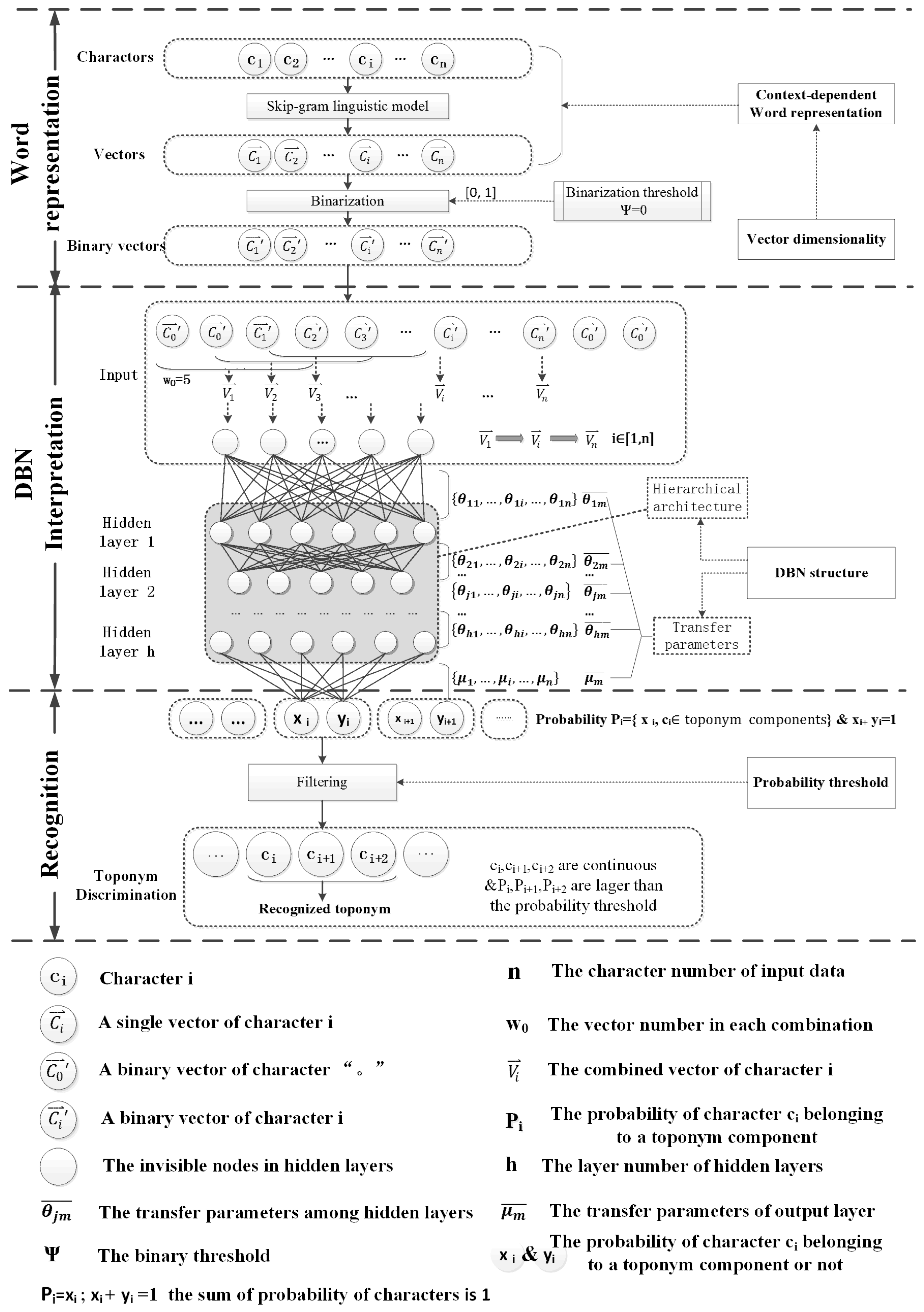
According to the two key issues from Section 2, our goal in this research is to improve the results of toponym recognition by using the Skip-Gram model, considering contextual information on the word representation process, and evaluating the relationships between the hyper-parameters of the DBN structure and the performance. The general framework is shown in Figure 1, which consists of three main stages: word representation, DBN interpretation and recognition. Firstly, word representation transforms characters into binary vectors , which can be composed into , the input form of the DBN structure. In this stage, we present the context-dependent Skip-Gram model and calculate the appropriate vector dimensionality. Secondly, DBN interpretation is described to show how to calculate the probability that each character belongs to a part of a toponym by using input vectors . Finally, the recognition process determines the recognized toponyms by using an optimized probability threshold and their continuity.
It should be noted that Chinese toponyms differ from the English ones. English toponyms can be a word or consist of several words, e.g., “London is the capital of the United Kingdom.” The minimum unit in an alphabetic language system is a word with separators. When the DBN structure is used to recognize English toponyms, each word can be transformed into vectors. However, Chinese toponyms can be a Chinese character or consist of several Chinese characters, e.g., “闵是福建省的简称。(Min is short for Fujian Province)”. A Chinese character is the minimum unit in Chinese sentences. Therefore, Chinese characters need to be transformed into vectors when the DBN structure interprets Chinese sentences.
3.1. Context-Dependent Word Representation
In general, toponym recognition belongs to classification problems, in which one needs to evaluate whether Chinese characters are toponyms or not. However, Chinese characters cannot be directly calculated in a DBN model. It is because DBNs compose of stacked Restricted Boltzmann Machines (RBMs), which was proposed based on Random Neural Networks (RNN) [38]. Every neuron in RNN has two probability-determined states, active or inactive, which are represented by 0 and 1. That means each neuron in DBNs also requires to be set to binary values. Therefore, Chinese characters cannot be directly calculated in a DBN model. The first step in recognizing toponyms in text is converting Chinese characters to binary vectors, which are the input form of the DBN model. Different toponym recognition approaches that are based on DBNs usually use different word representation models. Our goal is to obtain context-dependent binary vectors that represent various features of characters.
We assume that similar characters occur in similar contexts; in other words, that character representation is relevant to context [39]. This means we can obtain the appropriate representation of characters maximizing the probability of its context. This is a typical Skip-Gram model. Let represent the i-th character in document . The probability of the context of can be expressed as follows:
We construct an objective function by using a log function to calculate the maximum probability. Thus, the calculation of the maximum value of objective function is transformed into the calculation of the probability of around :
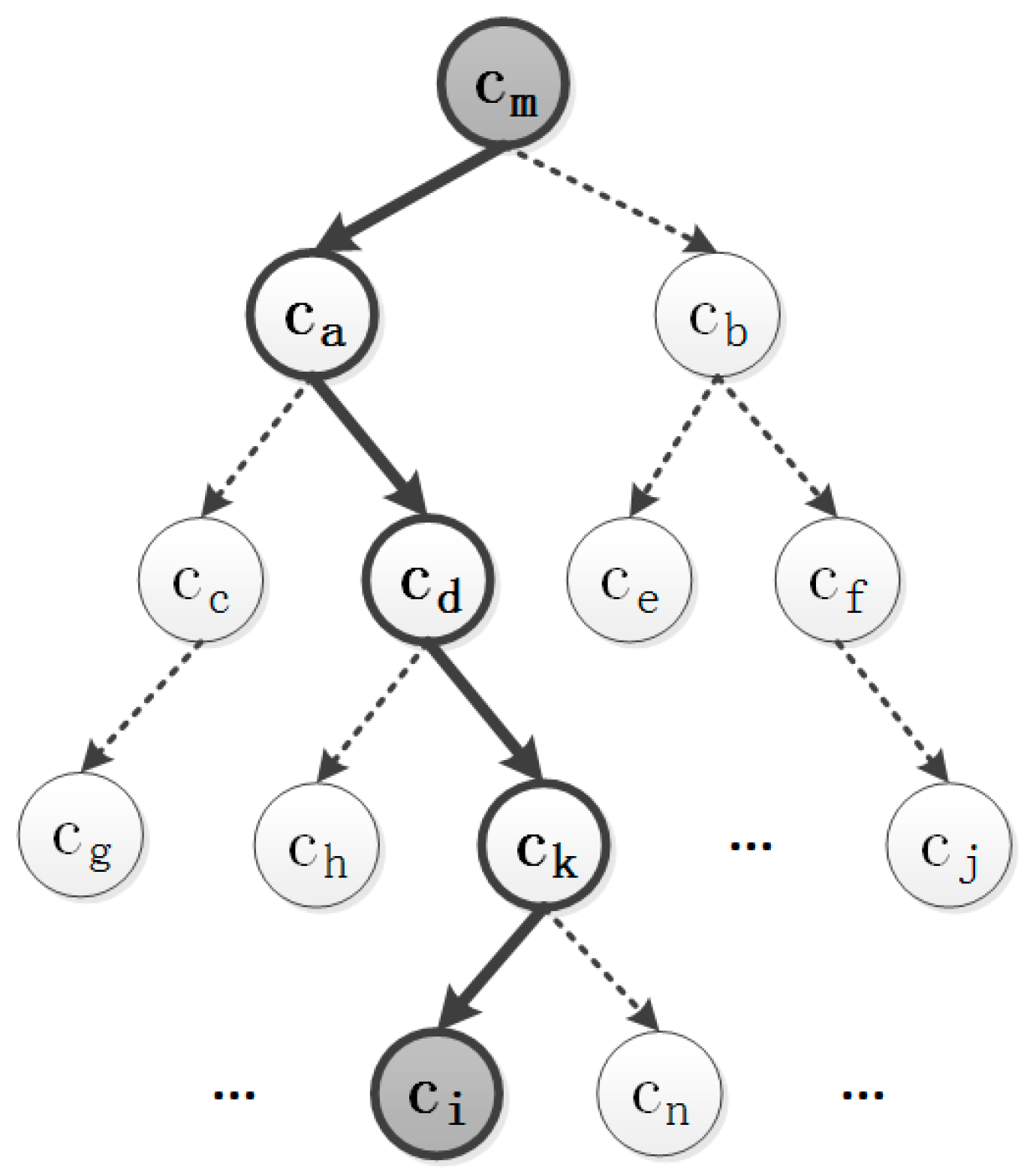
To solve this problem, we use an open-source tool named Word2Vec published by Google [28,40,41]. The Word2Vec tool calculates the maximum value of in an easier method. The main idea of this solution method is to transform this calculation into the calculation of binary classification probabilities in a character-frequency-weighted Huffman tree [28].
This solution lets each object character in the document have a specific path to achieve from the root character (Figure 2). is the character in the document with the highest frequency. Each node in that Huffman tree can be seen as a binary classification problem. Therefore, the probability of the object character can be calculated as follows:
And is a simple binary classification probability, which can be calculated by using classic logistic regression function [13].
When we obtain the maximum value of the objective function, we can obtain a unique list of feature vectors as well. There is a one-to-one correspondence between each character and each -dimensional feature vector . This process maps linguistic features of characters to -dimensional spaces of feature vectors. Thus, the feature vectors that are generated in this way contain the context-dependent linguistic features of characters. Then, the feature vectors should be transformed into binary vectors to suit the input form of the DBN structure.
3.2. Vector Dimensionality
Vectorization represents linguistic features in a vector space by using numbers. For instance, a d dimensional binary feature vector represents the Chinese character “市 (city)”. Thus, the linguistic features of characters are hidden in numbers that are uninterpretable to humans. Compared with traditional linguistic features, e.g., character features, context features or syntax features, these feature vector numbers are more abstract representations of linguistic features.
The dimensionality of the feature vector can be used to measure linguistic features. In general, the larger is, the richer the semantic information of the stored characters. A very high dimensionality requires an excessive consumption of computing resources and a very low dimensionality limits the presentation of linguistic features, which can directly affect the performance of toponym recognition. In principle, the performance of toponym recognition is a function of dimensionality :
where denotes the function of , is the interval of and and are the boundary values of the interval. It is noted that is not necessarily a monotonic function. To calculate a suitable vector dimensionality, the relationship between the vector dimensionality and performance needs to be determined experimentally (see Section 5.2 for details on how this was determined). Defining the range of possible values of to be considered, i.e., the interval , is a key step in this process.
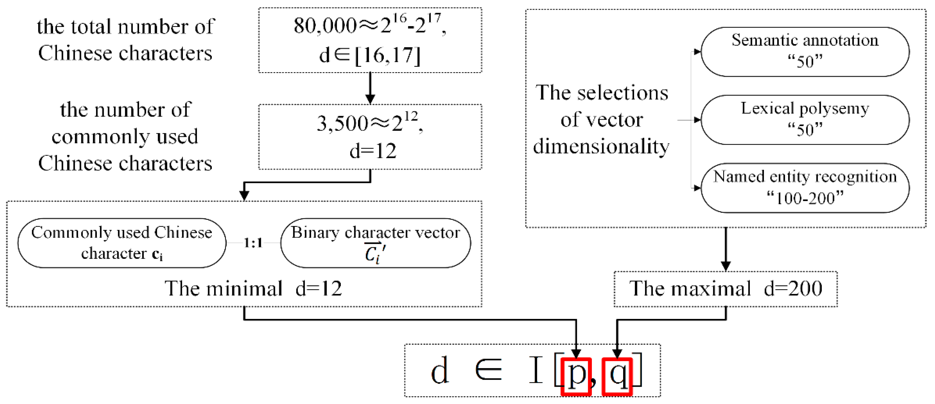
Figure 3 illustrates the selection of the dimensionality interval boundaries and . The lower limit can be estimated by the number of characters from the input text, with each character corresponding to a unique location in the vector space, i.e., the only information that is stored is the character that we are considering. For example, the total number of Chinese characters is approximately 80,000 (≈216 − 217) and the number of commonly used Chinese characters is approximately 3500 (≈212). A minimum vector dimensionality is needed to ensure that each commonly used Chinese character corresponds to at least one binary character vector. Thus, the lower limit of the interval should be set to 12. is the upper limit of the interval, which determines the highest vector dimensionality. It can be estimated by referring to the maximal dimensionality that is employed in similar deep-learning applications, which range from, e.g., 50 in semantic annotation [24], 50 in lexical polysemy analyses [42], and 100–200 in named entity recognition [27]. Thus, the interval was set to [12, 200].
3.3. DBN Structure
DBN interpretation depends on two key parts: a hierarchical architecture and transfer parameters. The former determines the depth and density of the structure and influences the abstractness and granularity of the feature interpretation; the latter represents the specific parameters of the interpretation process. Thus, the determination of the DBN structure can be divided into two parts.
a. Hierarchical architecture
The hierarchical architecture is mainly defined by the number of layers and the number of nodes within each layer and influences abstractness and granularity separately. The number of layers determines how many times the input feature vectors will be transferred. The more times they are transferred, the larger the abstract feature space that they can use will be. The number of nodes determines how many features the input feature vectors will represent. Thus, the number of nodes represents the feature granularity in DBN interpretation. These variables are generally determined from empirical knowledge [43]. We assume that these two variables affect the recognition performance, which denote as a function . Let and represent the number of layers and the number of nodes. A greedy algorithm can be used to determine the two variables [15]. Following Equation (5), the partial derivatives are computed for each hyper-parameter:
In general, there is a convergent correlation between the recognition performance and the architecture in terms of the numbers of layers and nodes [44]: more layers and nodes improve the performance up to a point; then the performance stablilizes. Therefore, hierarchical architecture hyper-parameters can be identified by analysing this convergent relationship with experimentation.
b. Transfer parameters
After determination of the hierarchical architecture, the calculation of transfer parameters then seeks to find the best inner path from the input data to the output data. The parameters include , which is the parameter between the input layer and the hidden layer h; and , which is the parameter of the output layer; here, m represents the number of characters in the training data. In general, these parameters can be calculated by the classic wake-sleep algorithm [45], which includes a pre-training stage and a fine-tuning stage. The wake-sleep algorithm can effectively improve the convergence speed and reduce the final inference error [46,47]. In the pre-training stage, the stacked RBM structures are trained in sequence. For each layer, the transfer parameters can be calculated as follows with a commonly used small gradient value of 0.2 with a deviation of less than 0.1:
where denotes the transfer parameter of hidden layer h of the i-th input character vector, is the input layer, and is the output of the probability distribution of . For wake–sleep algorithms, the energy equation and Gibbs sampling approach are used to calculate the descent gradient. The partial derivative is computed as follows [48,49]:
In the fine-tuning stage, the output layer can be regarded as a single layered neural network, and a back-propagation algorithm can be used to set the transfer parameters.
3.4. Probability Threshold
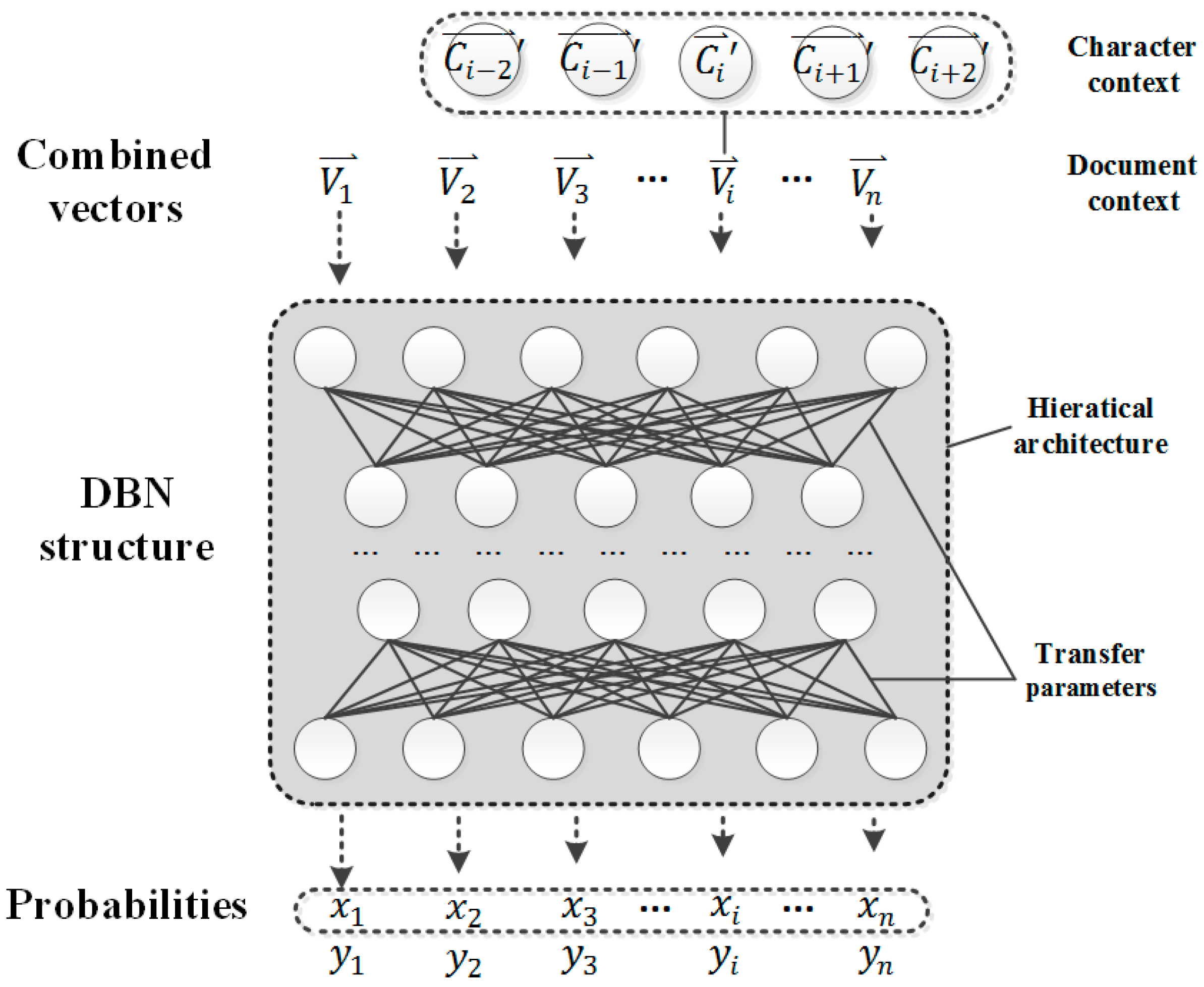
The process of interpretation of linguistic features results in a toponym probability value for all characters. To select a character as part of a toponym, an optimal threshold value for the probability is selected. Figure 4 shows the processes of toponym recognition after the application of the DBN structure, and indicates that the probability threshold is key to identifying whether a character belongs to a toponym component. A very high threshold decreases the number of toponyms that are recognized. In contrast, a very low threshold results in lower accuracy of toponym recognition. Thus, the probability threshold determines toponym recognition performance.
Let represent the probability threshold. The probability of toponym recognition for whole input texts can be expressed as follows:
The notations for Equation (8) are listed as follows:
- : the set of characters in the text;
- : character i in the text;
- : toponym i;
- : the probability that character i belongs to a toponym component.
Generally, the selection of the probability threshold is achieved with a maximum likelihood estimation process. By adding logarithms of probabilities instead of multiplying probabilities, to avoid underflows, the computation process for the likelihood value is transformed as follows [50]:
An optimal threshold can be determined with a partial derivative by a gradient descent search (see Section 5.2 for details), where Equation (9) obtains the maximum value.
4. Experiments
4.1. Framework
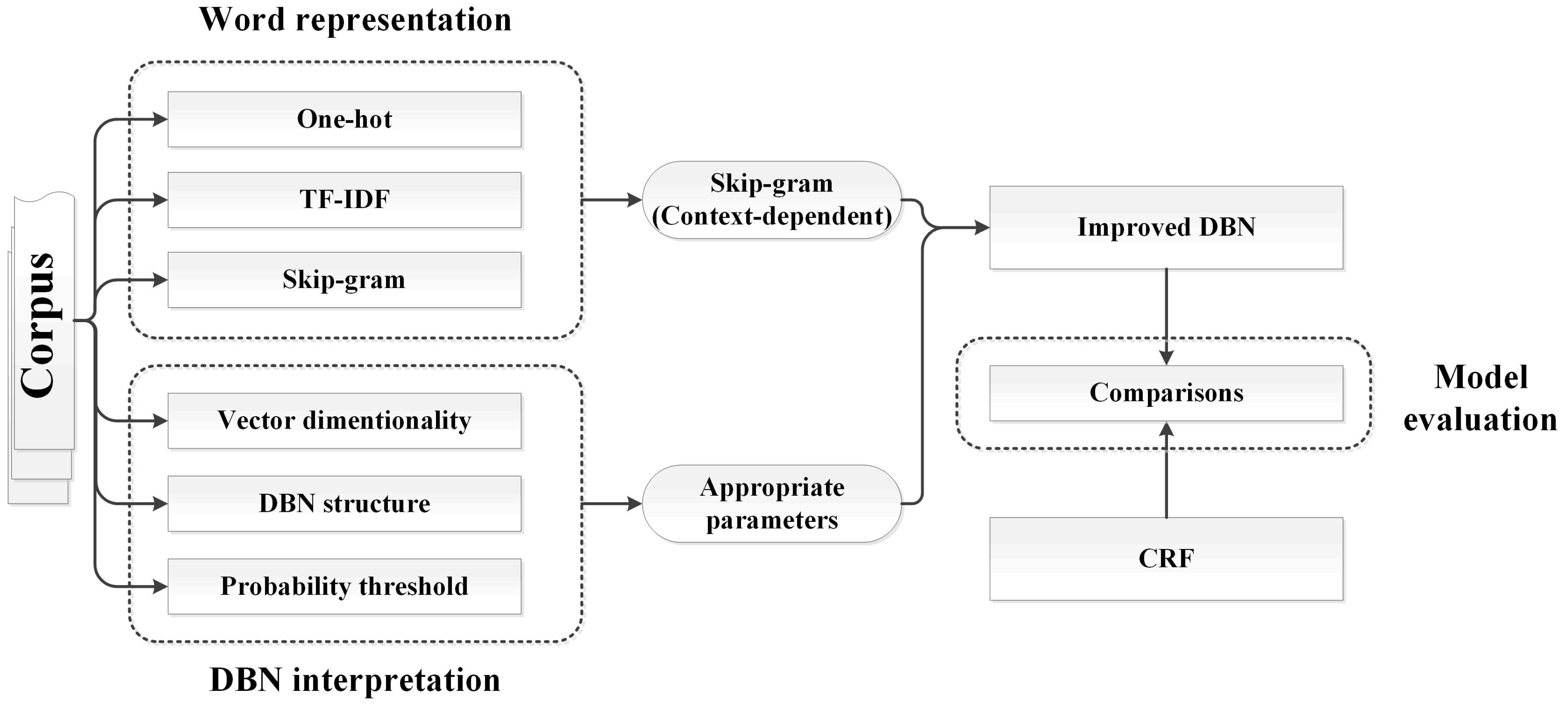
The experimental framework is shown in Figure 5. Experiments on word representation are used to evaluate the performances of word representation models, which are used in the DBN-based toponym recognition approach. Experiments on DBN interpretation analyse the relationships between the performance and the hyper-parameters of DBN interpretation by using univariate experimentation. The final experiments are used to evaluate the performance of the improved approach compared with a state-of-the-art CRF model.
4.2. Datasets
a. Encyclopedia of China: China Geography (ECCG) corpus
Encyclopedia of China: China Geography (ECCG) is a geographical treatise, which provides detailed information on topography, climate, hydrology, natural resources, and administrative areas. The ECCG corpus is an annotated geographical Chinese corpus, which contains nearly 2.13 million Chinese characters and over 0.12 million toponyms in over 1600 documents [51]. These documents have a higher frequency of toponyms than other universal corpus’, e.g., 0.03 million toponyms in 3.20 million Chinese characters in ACE2004 [8], 0.02 million toponyms in 1.2 million Chinese characters in a 20-Newsgroups corpus [9], and 0.04 million toponyms in 5.0 million toponyms in a Sogou corpus [11]. The whole ECCG corpus was shared with the Chinese Linguistic Data Consortium in 2015 [52].
In the ECCG corpus, each toponym consists of at least one Chinese character and at most nine Chinese characters, and belongs to one of four main types: area, water, landscape and transport. The distribution of the ECCG corpus is described in Table 1. Each toponym consists of several Chinese characters and each Chinese character can be regarded as a single input element. For example, the Chinese sentence “紫金山位于南京市东部。” (Zi Jin Mountain is located in Eastern Nanjing.) includes two highlighted toponyms. The first toponym consists of the Chinese characters “紫” (Zi), “金” (Jin) and “山” (Mountain), each of which is represented in the vector space during the interpreting process.
b. Annotation
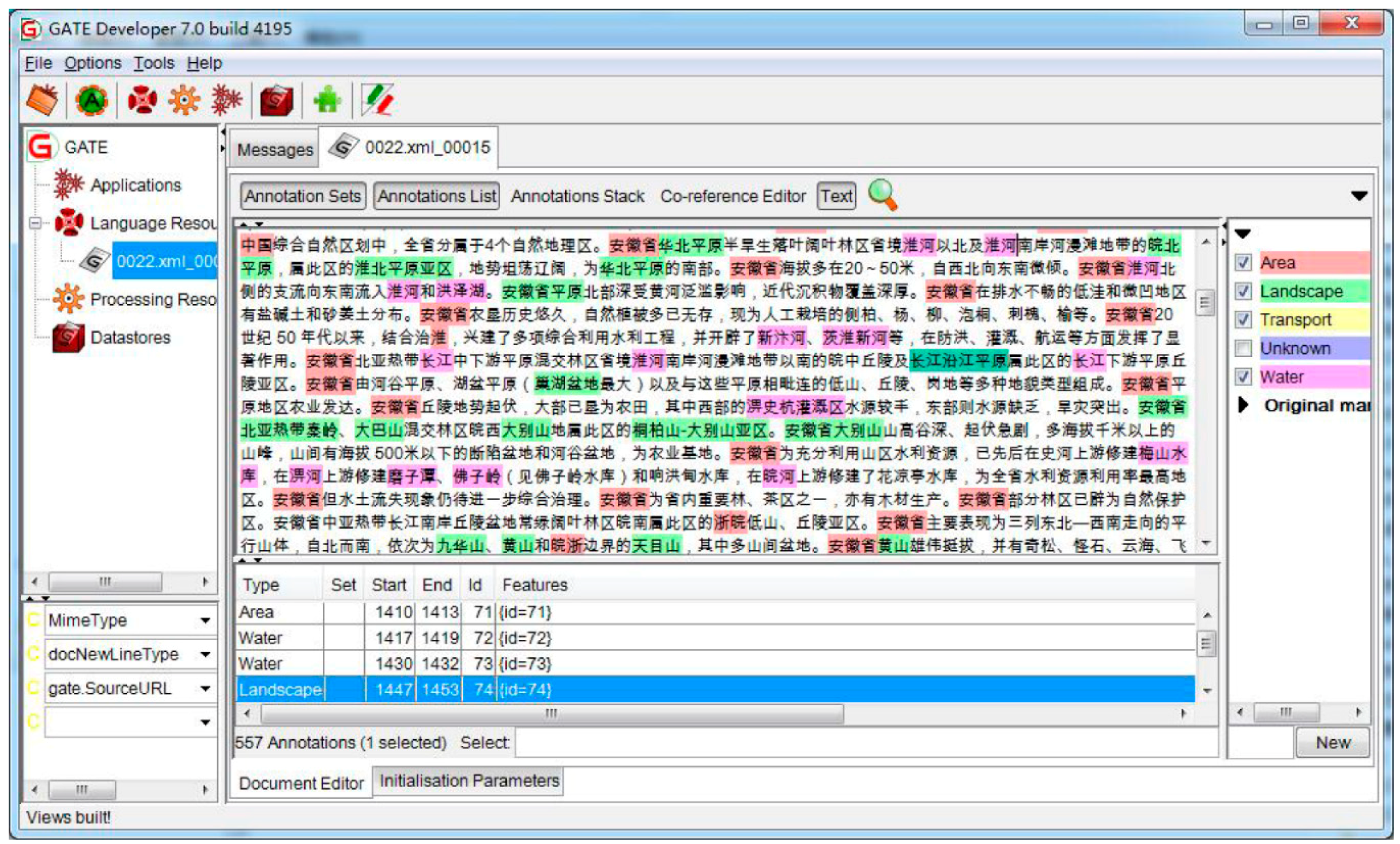
The ECCG corpus was annotated and cross-verified by using GATE, which is a development environment that provides aids for construction, testing and evaluation of Language Engineering (LE) systems [53]. It is noted that all the toponyms in different types need to annotate orderly in manual. A fine annotated ECCG document is shown in Figure 6. There are 557 toponyms on four types (area, landscape, transport and water) in a document file with 8000 Chinese characters.
c. Training and Testing
The training and testing dataset was extracted into five sequential subsets to explore the relationship between the variables and the performance on datasets of different sizes (0.1 million Chinese characters to 2.0 million Chinese characters, with an interval of 0.1 million Chinese characters). On each subset, 10-fold cross validation was performed with 20% of the training data.
4.3. Evaluation Measures
The performances of toponym recognition can be evaluated using the following measures. Precision (P) is the fraction of toponyms that are correctly recognized. In Equation (10), C denotes the number of toponyms that are correctly recognized and T represents the total number of characters that are identified by the system as parts of toponyms. Recall (R) is the fraction of annotated toponyms that are correctly recognized. In Equation (11), A denotes the total number of labelled toponyms. The F value in Equation (12) is the harmonic mean of precision and recall. In general, it is used to evaluate the validity of a recognition approach. The F value can be simplified to the F1 value in Equation (13), by setting . The statistical significance of these measures can be verified by using randomization on different methods [54]:
4.4. Implementation Details
In the word representation stage, the Skip-Gram model is implemented by using word2vec, which is an open-source word representation tool that was published by Google [40]. Considering that characters are the minimal unit in ideographic languages, we transform each Chinese character in the experimental corpus into a binary feature vector. The window size of word representation is set to 5, which is a commonly used window size that is suitable for the Skip-Gram model. The DBN interpretation process is implemented by modifying the “DeepLearning” repository from GitHub (https://github.com/yusugomori/DeepLearning), using ideas that were discussed in Section 3. All our experimental codes are implemented in the Java and are publicly available in GitHub (https://github.com/shuwang8951/TRcode).
5. Results
In this section, we evaluate our model in three experiments: an evaluation of word representation models, an analysis of the hyper-parameters of DBN interpretation and a comparison to a state-of-the-art CRF model. We will describe these experiments in detail in the following sections.
5.1. Word Representation Model
To confirm the validity of the proposed word representation models, the Skip-Gram model is compared with One-Hot word representation model [8] and the TF-IDF model [11], which are used in the previous DBN approach. In addition, the ACE 2004 corpus that is used by the One-Hot model and the Sogou corpus that is used by the TF-IDF model are universal corpora, which focus not only on toponyms. Both these corpora have lower toponym frequencies than the ECCG corpora (0.12 million toponyms within 2.13 million Chinese characters). Therefore, we designed two separate experiments: an experiment on different word representation models to verify sentence-level context information of the Skip-Gram model and an experiment on different training corpora to estimate whether the toponym frequency affects the performance.
a. Experiment on different word representation models
At present, different toponym recognition approaches that are based on DBNs use different word representation models. In this part, we list the results of the One-Hot representation model, TF-IDF model and Skip-Gram model in Table 2. Groups 1, 2 & 3 explore the performance on different representation models, e.g., One-Hot, TF-IDF and Skip-Gram, with the Chen’s DBN structure on the ECCG corpus. In addition, groups 4, 5 & 6 explore the performance on different representation models, e.g., One-Hot, TF-IDF and Skip-Gram, with the improved DBN structure (see Section 5.2) on the ECCG corpus. Groups 1 & 4 compare the differences on different DBN structures with the One-Hot representation model. In addition, groups 2 & 5 and groups 3 & 6 are for the TF-IDF and Skip-Gram models, respectively.
Comparing groups 1, 2 & 3 with groups 4, 5 & 6, the F1 values increase by 0.0411, 0.0247 and 0.0543, respectively. The significant levels for F1 values are 0.0048, 0.0031 and 0.0053, respectively. It is shown that regardless of the DBN structure, Skip-Gram models outperform One-Hot models and TF-IDF models. Moreover, comparisons of groups 1 & 4, groups 2 & 5 and groups 3 & 6 indicate that the improved DBN structure outperform one of the typical DBN structures.
Furthermore, the recognition results of the experiments are analysed to determine which parts of the results are improved by using a Skip-Gram model. The main improvement is achieved at the boundaries of long continuous toponyms; for example, in the sentence “八松错地处林芝地区工布江达县境内。” (Basong Cuo is located on Gongbu Jiangda country, Linzhi District), the One-Hot representation and TF-IDF models cannot recognize the toponyms of “林芝地区 (Linzhi District)” and “工布江达县 (Gongbu Jiangda country)”. The recognition of these long continuous toponyms requires contextual information. Thus, it is confirmed that the Skip-Gram model of word representation retains the context-dependent information and optimizes the toponym recognition performance for long continuous toponyms.
b. Experiment on different training corpora
In the experiments, two kinds of DBN-based toponym recognition approaches are considered: Chen’s approach [8] and our proposed approach. Chen’s approach uses a One-Hot word representation model and a fixed DBN structure (One-Hot+ fixed DBN). Our proposed approach uses a Skip-Gram word representation model and an adjusted DBN structure (Skip-Gram+ our DBN). The results are listed in Table 3.
In Group 1 and Group 2, two DBN models were evaluated on the ACE 2004 corpus and ECCG corpus, respectively. In Group 3, the two models were evaluated on the ACE 2004 corpus after training on the ECCG corpus. The proposed approach achieved improvements in either precision or recall on these three groups. The results indicate that the corpus is one of the key factors that influence toponym recognition. This is confirmed by two comparative experiments: (i) In Group 3 and Group 1, Chen’s approach obtained a 0.1047 decrease of F1 value and the proposed approach obtained a 0.0261 decrease of F1 value by changing training corpus from ECCG to ACE 2004, which has sparse toponyms. This means that the corpus with lower toponym frequency negatively affects the training of the DBN model. (ii) When the training corpora have adequate toponym frequencies, the testing corpora will affect the performance. In Group 2 and Group 3, the two DBN models achieve performance improvements with different testing corpora, which proves that different kinds of testing corpora result in different performances.
In this paragraph, we analyse the recognition results on Group 2. As the two models have similar recognition mechanism, most of the results are similar (Table 4). They are sensitive to trigger Chinese characters. For example, in the sentence “安徽省的乡镇工业将会有较大发展。” (The village and township industry in Anhui will be greatly developed), both of the models correctly recognize the toponym of “安徽省” (Anhui), but they incorrectly recognize the toponym “乡镇” (village and township). Neither DBN model can distinguish these typical Chinese characters.
However, in the results of these two DBN models, there exists some differences. The main kind of difference is in the recognition of the descriptions of long toponyms. Chen’s DBN model cannot recognize the boundaries of long toponym descriptions clearly. For example, in the sentence, “安徽省亚热带混交林区位于淮河南岸。” (Anhui subtropical mixed forest region is located on the south bank of the Huaihe river), Chen’s approach recognized two toponyms “安徽省” (Anhui) and “交林区” (forest region). It cannot recognize toponyms that consist of more than seven Chinese characters. This means that the evaluated variables compensate for the weakness of Chen’s DBN model. The proposed DBN model can recognize linguistic features with long toponym descriptions.
5.2. Effects of the Hyper-Parameters on the DBN Interpretation
a. Vector dimensionality
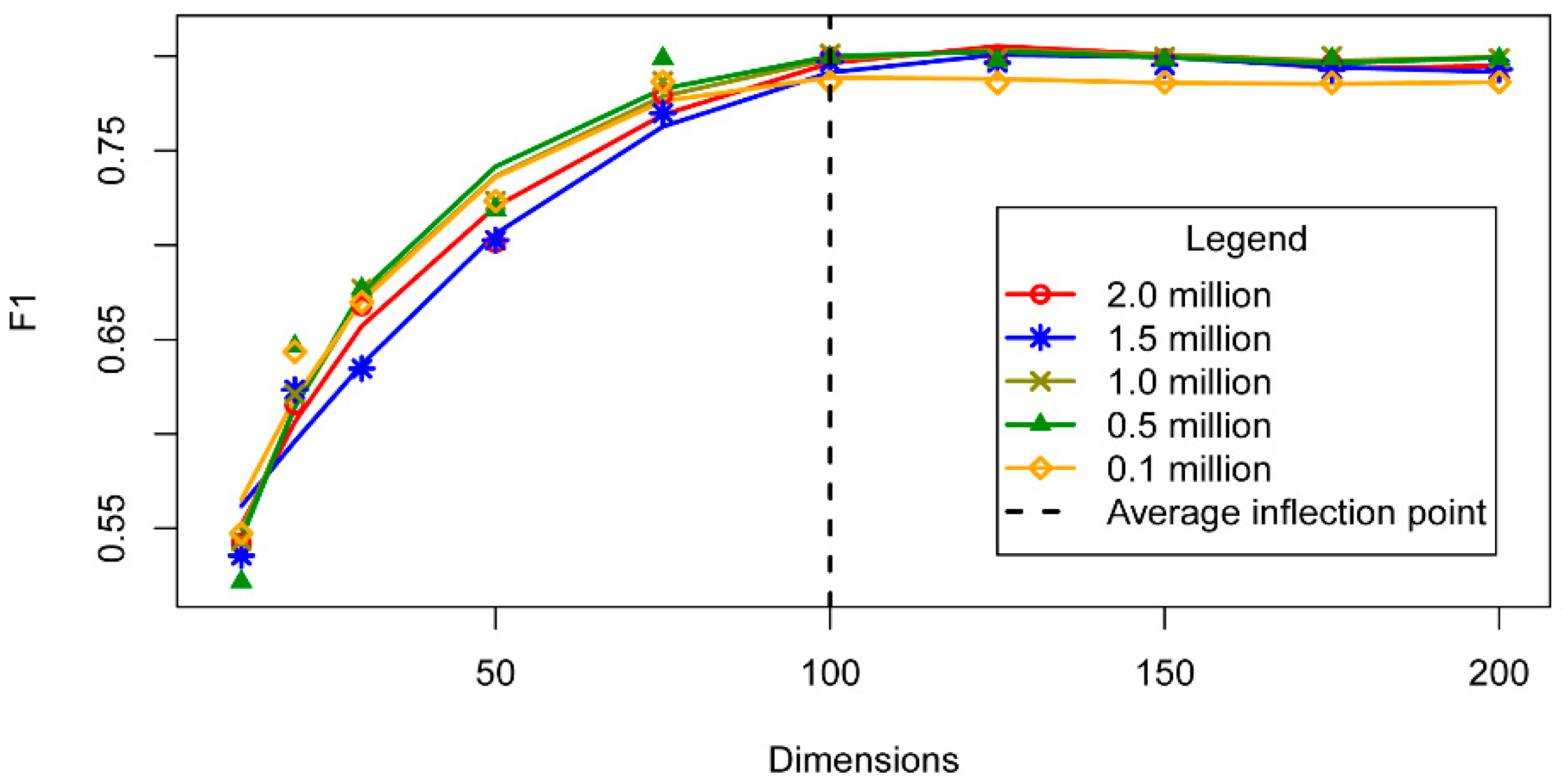
The vector dimensionality was determined by analysing the relationship between the dimensionality and the toponym recognition performance within the interval [12, 200] for each of the differently sized datasets. Figure 7 shows that the F1 value increased rapidly in the interval [12, 100] and remained stable in the interval [100, 200] as the dimensionality increased. The relationship between the two variables clearly converged in the interval. Figure 7 illustrates the appearance of an inflection point at approximately a dimensionality of 100, after which F1 maintains a stable value with no gain, while requiring extra computation. Hence, the dimensionality was set to 100 in this study.
b. DBN hierarchical architecture
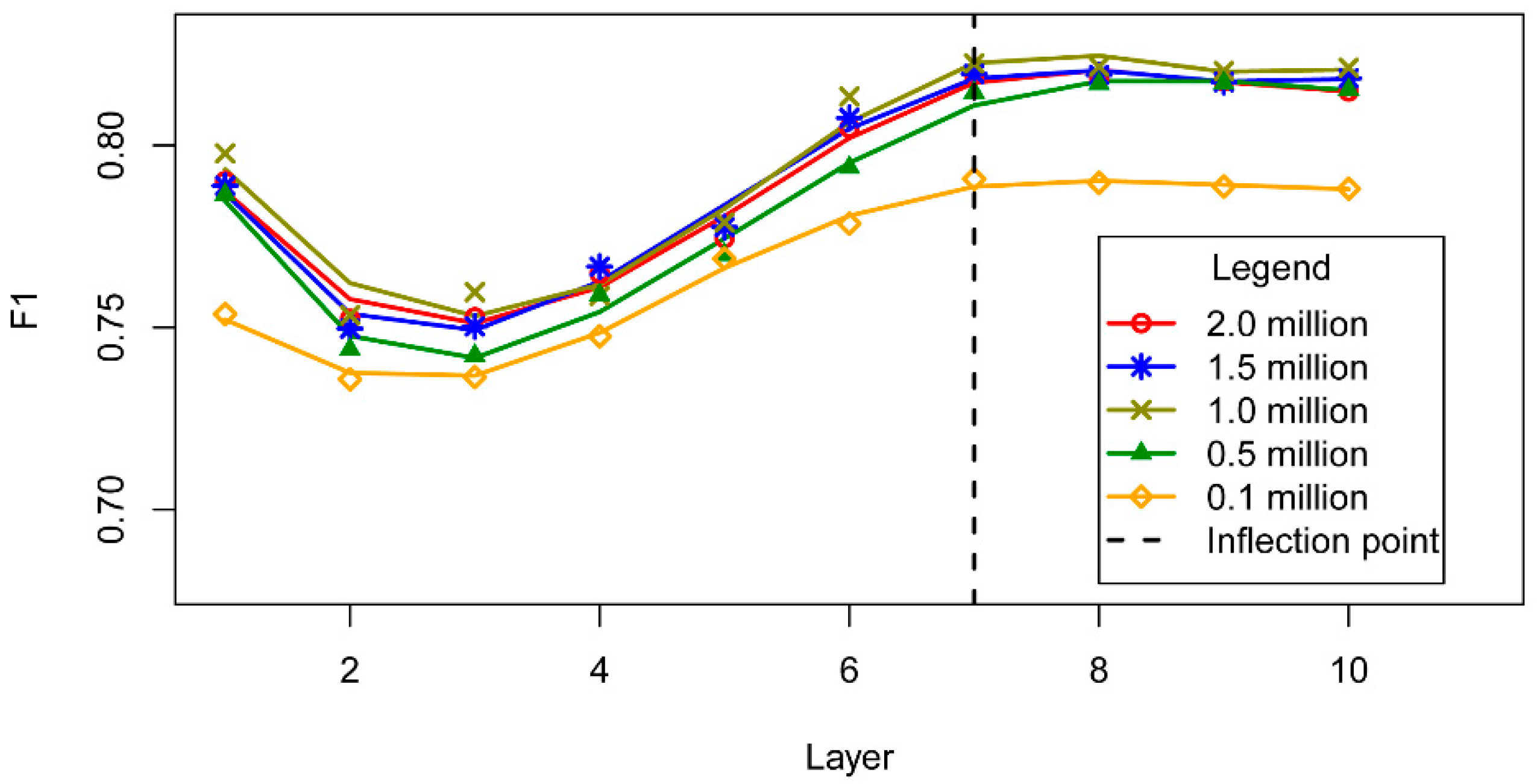
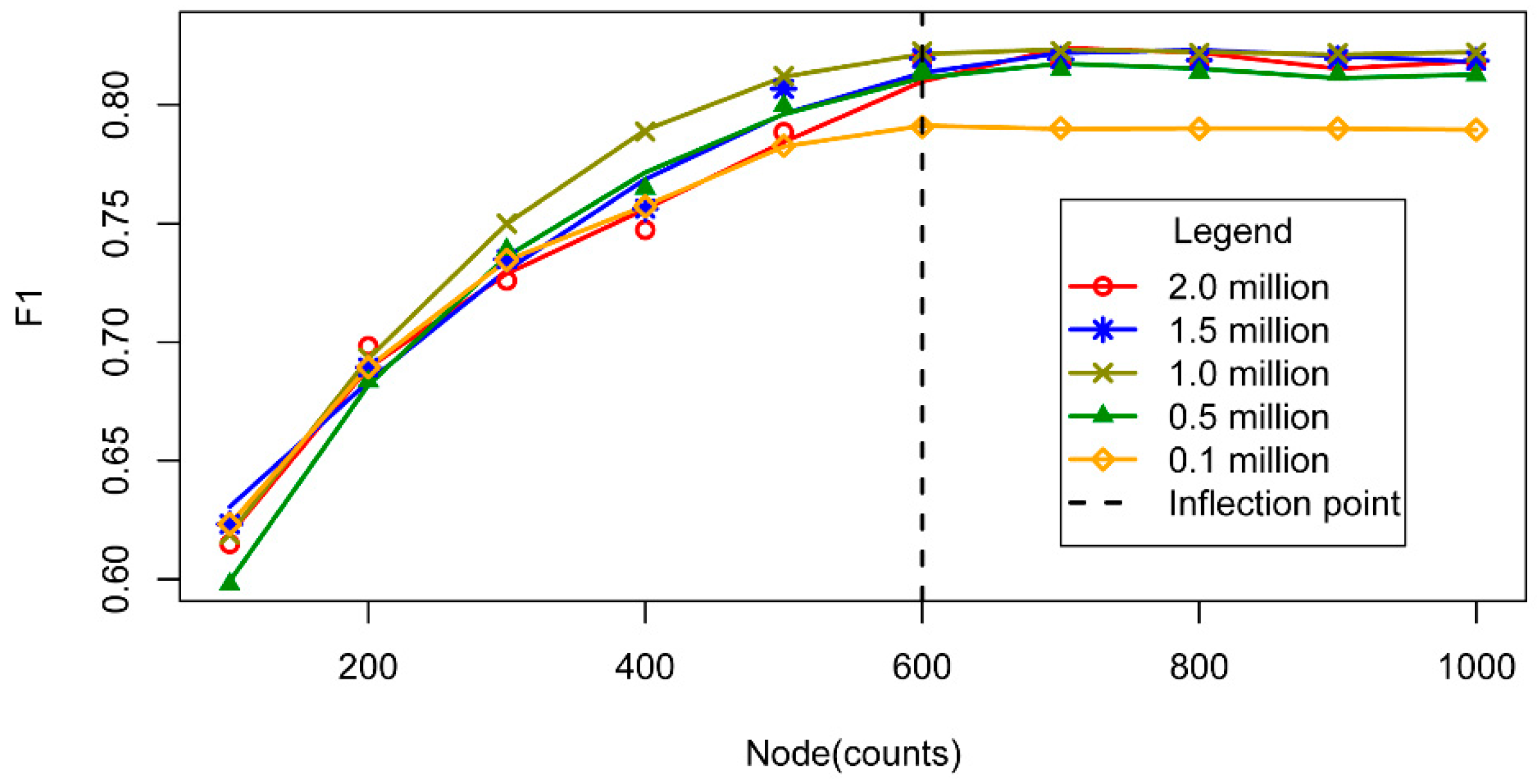
To calculate the number of layers and the number of nodes, experiments were performed to analyse the relationship between the two variables and the performance of the toponym recognition procedure. Figure 8 illustrates the general trend of the F1 value against the number of layers, which decreased initially and then rapidly rose with the number of layers before stabilizing when the number of layers exceeded 7. With the number of nodes increasing, as shown in Figure 9, the F1 value peaked and levelled off for values of more than 600 nodes. The two trends remained steady. Thus, the number of layers and the number of nodes were set to 7 and 600, respectively.
c. Probability threshold
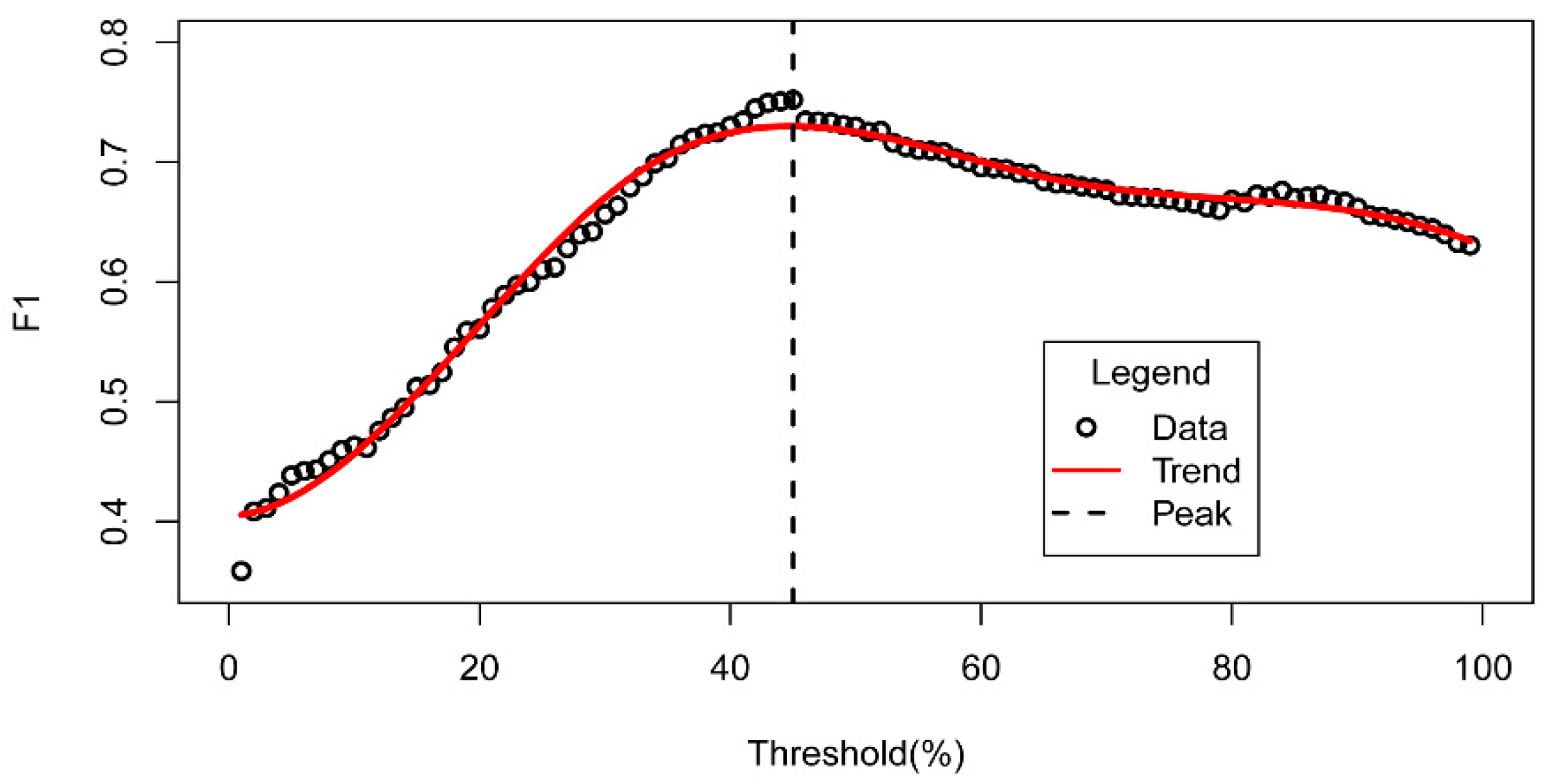
During the process of toponym recognition, the sampling value of gradient descent was set to 0.01, which led to an average rate of change of the F1 value of less than 0.005. Figure 10 presents the relationship between the thresholds and F1 values. The results show that the F1 value increased rapidly and then decreased gradually. When the threshold reached 0.45, the F1 value also reached its peak. Thus, the probability threshold was set to 0.45.
5.3. Comparison with a CRF Model
In this part, the experiments will compare the proposed toponym recognition approach and a state-of-art CRF-based approach [32] on the same corpus, namely, ECCG. The CRF-based approach follows the basic processes in Figure 11. Training data are used to extract features by considering 1-gram character chunks, frequency statistics and syntax analyses with expert linguistic experiences. The extracted basic features in the CRF model are of six main types, which are listed in Table 5. Features 1, 2 & 4 contain the fundamental character information, which are basic features in the CRF model. Features 3, 5 & 6 are selected based on previous research, which can effectively improve performance. The CRF model can be trained by using these linguistic features and in the recognition process, the toponyms can be extracted with this trained CRF model. The processes of the CRF model were implemented by using the open source CRF++ tool.
As the performance of the machine-learning models correlates directly with the corpus size, a large training corpus contains more linguistic features that are associated with toponyms, which allows the methods to achieve a more accurate model with higher precision and recall. To determine the experimental dataset on the DBNs and the CRF, our experiments explored F1 trends on different corpus sizes.
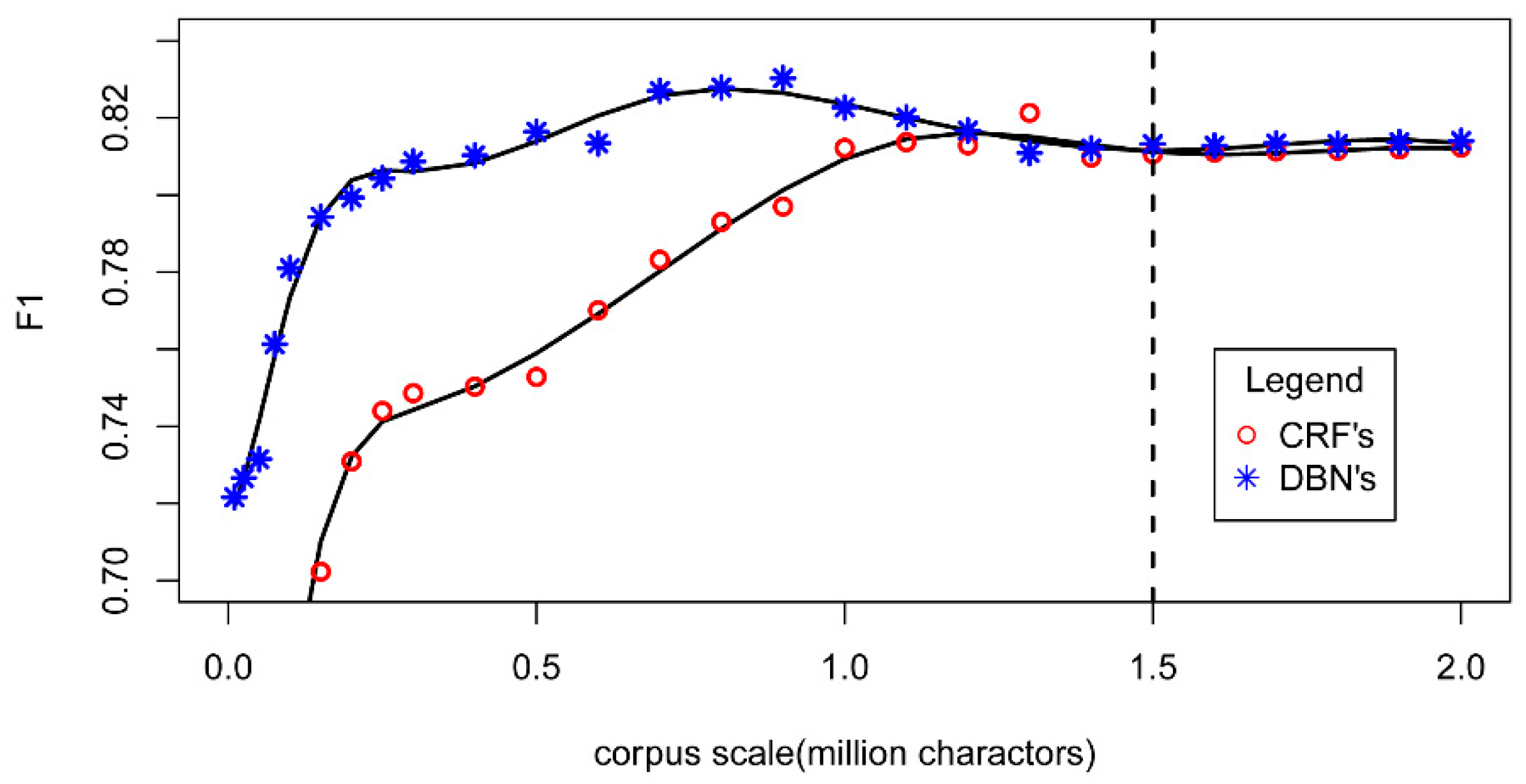
The F1 trends of the DBNs and CRF on different corpus sizes are shown in Figure 12. Overall, the F1 values increased with corpus size. With DBNs, the trend increased sharply with the corpus size, until it reached approximately 0.25 million. After that rapid increase, the values increased slowly, reaching the highest values for a corpus size of 1.0 million and finally stabilizing for sizes above 1.5 million. However, the increase in F1 values for CRF was slower than that of DBNs. The trend achieved its peak for a corpus size of nearly 1.3 million before stabilizing. Two clear observations are made from the results: (i) For small corpus sizes (<1.0 million), the DBNs outperformed the CRF. Thus, the DBNs can be trained with smaller corpora; (ii) When the corpora are larger, there are no obvious differences between these two models.
Table 6 lists the performances of the DBNs and the CRF for toponym recognition on the full corpus size of 2.0 million. The results showed that the DBN model achieved a slightly-higher recall (0.0115 with the significant level of 0.0003) and a slightly lower precision (0.0052 with the significant level of 0.0012) in comparison with the CRF model. The F1 value increased 0.0037 at the significant level of 0.0018. To our surprise, the overall results of the proposed approach and the CRF model are approximately the same (F1 ≈ 0.80).
Although no significant overall differences were observed between the DBN and the CRF results, the specific toponym recognition results of the two models were not the same. In the CRF, there were two main kinds of errors: (i) Abbreviation descriptions were not recognized. For example, in the sentence “江苏省简称苏。” (Su is shortened to Jiangsu province), CRF cannot recognize the toponym “苏” (Su). (ii) Long toponyms were not recognized. For example, in the sentence “安徽省亚热带混交林区位于淮河南岸。” (Anhui subtropical mixed forest region is located on the south bank of the Huaihe river), CRF cannot recognize the long toponym of “安徽省亚热带混交林区”. For the DBN, there were two different kinds of errors: (i) Continuous toponyms were not recognized. For example, in the sentence “大庆、东营、盘锦、松原、克拉玛依、潜江是中国典型的石油城市。” (Daqing, Dongying, Panjin, Songyuan, Kelamayi and Qianjiang are the typical petroleum cities in China), DBNs would commonly miss some Chinese characters. The recognition results of this sentence were “大庆” (Daqing), “东” (Dong), “盘锦” (Panjin), “松原” (Songyuan), “克拉玛” (Kelama), “潜江” (Qianjiang) and “中国” (China); (ii) Trigger Chinese character descriptions are incorrectly recognized. For example, in the sentence “苹果、红枣、海参、鲍鱼等是山东的特产。” (Apple, date, sea cucumber and abalone are specialty products of Shandong), DBN recognizes two toponyms: “海” (sea) and “山东” (Shandong). However, Chinese character “海” (sea) is recognized incorrectly because it is a high-frequency trigger character of toponyms in Chinese. In summary, our adapted DBN-based toponym recognition approach prefers abbreviated characters and sentence-level context information, whereas CRF models recognize more trigger characters and boundaries.
These specific recognition results demonstrate that these two types of models differ in their mechanics. CRF models exploit manually specified linguistic features of toponyms, whereas the DBN model uses its network architecture to learn deep, abstract linguistic features. Table 7 lists the recognition errors and their relevant linguistic features. Abbreviation descriptions and long toponym descriptions, which can be well recognized by DBNs, correspond context-dependent linguistic features. Conversely, continuous toponyms and trigger Chinese character descriptions correspond to single linguistic features, which have been selected by CRF models. This means that a CRF can train models well, based on selected linguistic features. In addition to the above issues, DBNs can capture additional hidden linguistic features, which might consist of multiple linguistic features, from input data by their multi-layered structure.
To compare the specific recognition results of the two models further, our experiments identified differences among the recognized toponyms. Table 8 lists the different types of toponyms that are recognized by these two models. The relatively large number of recognized toponyms indicates a significant complementarity between the DBN and CRF models.
To investigate this further, we conducted experiments that combined the results of the DBN and CRF models. The combined results are listed in Table 6, which show that the combination of the two approaches improves the F1 performance of toponym recognition effectively. Thus, although the combined precision decreased by nearly 0.03 at the significance of 0.0015, the recall rate increased by approximately 0.16 at the significance of 0.0027, from approximately 0.77 to more than 0.93, and the resulting F1 value increased by approximately 0.06 at the significance of 0.0012. All these differences are statistically significant.
6. Conclusions
In this paper, we investigated an adapted DBN-based toponym recognition approach by using a Skip-Gram word representation model that takes into account contextual information. In addition, we identified the relationships between hyper-parameters of DBN interpretation and performance, and determined their stable values. Our experiments evaluated our approach and compared it with the state-of-the-art CRF model.
The experimental results show that the DBN model outperforms the CRF model with smaller corpus (<1.0 million characters). When the corpus size is large enough (>1.5 million characters), their statistical metrics become closed (P ≈ 0.81, R ≈ 0.77 and F1 ≈ 0.80). However, their recognition results express differences and complementarity on different kinds of toponyms, especially for abbreviated and long toponym descriptions. More importantly, combining their results can directly improve the performance of toponym recognition relative to their individual performances (P ≈ 0.79, R ≈ 0.94 and F1 ≈ 0.85). The experiments illustrate that the scale of the corpus has an obvious effect on the performance of toponym recognition. And generally, there is no adequate tagged corpus on specific toponym recognition task, especially in the era of Big Data. In conclusion, we believe that the DBN-based approach is a promising powerful method to extract geo-referenced information from text in the future.
Author Contributions
Conceptualization, S.W. and X.Z.; data curation, S.W.; formal analysis, S.W.; funding acquisition, X.Z.; methodology, S.W., X.Z. and M.D.; software, S.W. and P.Y.; supervision, X.Z.; validation, P.Y. and M.D.; writing—original draft, S.W.; writing—review & editing, M.D.
Funding
This research was funded by the National Natural Science Foundation of China grants No. 41631177 & No. 41671393 and the National Key Research and Development Program of China No. 2017YFB0503602.
Acknowledgments
The authors thank Christopher B. Jones, Andrew Evans, Junzhi Liu, Joshua Pohl and Jie Zhu for their critical reviews and constructive comments.
Conflicts of Interest
The authors declare no conflict of interest.
References
- Leidner, J.L. Toponym resolution in text: Annotation, evaluation and applications of spatial grounding. ACM SIGIR Forum 2007, 41, 124–126. [Google Scholar] [CrossRef]
- Jones, C.B.; Purves, R.S. Geographical information retrieval. Int. J. Geogr. Inf. Sci. 2008, 22, 219–228. [Google Scholar] [CrossRef] [Green Version]
- Hinton, G.; Deng, L.; Yu, D.; Dahl, G.E.; Mohamed, A.; Jaitly, N.; Senior, A.; Vanhoucke, V.; Nguyen, P.; Sainath, T.N. Deep neural networks for acoustic modeling in speech recognition: The shared views of four research groups. IEEE Signal Process. Mag. 2012, 29, 82–97. [Google Scholar] [CrossRef]
- Yu, K.; Lei, J.; Chen, Y.Q.; Wei, X. Deep Learning: Yesterday, Today, and Tomorrow. J. Comput. Res. Dev. 2013, 20, 1349. [Google Scholar]
- Collobert, R.; Weston, J.; Bottou, L.; Karlen, M.; Kavukcuoglu, K.; Kuksa, P. Natural language processing (almost) from scratch. J. Mach. Learn. Res. 2011, 12, 2493–2537. [Google Scholar]
- Huang, Z.; Xu, W.; Yu, K. Bidirectional LSTM-CRF Models for Sequence Tagging. Comput. Sci. 2015, arXiv:1508.01991. [Google Scholar]
- Lample, G.; Ballesteros, M.; Subramanian, S.; Kawakami, K.; Dyer, C. Neural Architectures for Named Entity Recognition. In Proceedings of the HLT-NAACL, San Diego, CA, USA, 12–17 June 2016; pp. 260–270. [Google Scholar]
- Chen, Y.; Ouyang, Y.; Li, W.J.; Zheng, D.Q.; Zhao, T.J. Using deep belief nets for Chinese named entity categorization. In Proceedings of the 2010 Named Entities Workshop, Uppsala, Sweden, 16 July 2010; pp. 102–109. [Google Scholar]
- Jiang, M.Y.; Liang, Y.C.; Feng, X.Y.; Fan, X.J.; Pei, Z.L.; Xue, Y.; Guan, R.C. Text classification based on deep belief network and softmax regression. Neural Comput. Appl. 2016, 29, 61–70. [Google Scholar] [CrossRef]
- Liu, T. A Novel Text Classification Approach Based on Deep Belief Network. In Proceedings of the International Conference on Neural Information Processing, Sydney, Australia, 22–25 November 2010; pp. 314–321. [Google Scholar]
- Song, J.; Qin, S.J.; Zhang, P.Z. Chinese text categorization based on deep belief networks. In Proceedings of the 2016 IEEE/ACIS 15th International Conference on Computer and Information Science (ICIS), Okayama, Japan, 26–29 June 2016; pp. 1–5. [Google Scholar]
- Nadeau, D.; Sekine, S. A survey of named entity recognition and classification. Lingvisticae Investig. 2007, 30, 3–26. [Google Scholar]
- Melo, F.; Martins, B. Automated Geocoding of Textual Documents: A Survey of Current Approaches. Trans. Gis 2017, 21, 1–35. [Google Scholar] [CrossRef]
- Moschitti, A.; Basili, R. Complex linguistic features for text classification: A comprehensive study. In Proceedings of the European Conference on Information Retrieval, Sunderland, UK, 5–7 April 2004; pp. 181–196. [Google Scholar]
- Hong, S.; Chen, J.J. Research on the Chinese Topontm recognition method with two-layer CRF and rules combination. Comput. Appl. Softw. 2014, 11, 175–177. [Google Scholar]
- Névéol, A.; Grouin, C.; Tannier, X.; Hamon, T.; Kelly, L.; Goeuriot, L.; Zweigenbaum, P. CLEF eHealth Evaluation Lab 2015 Task 1b: Clinical Named Entity Recognition. Available online: http://ceur-ws.org/Vol-1391/inv-pap5-CR.pdf (accessed on 20 April 2018).
- Bikel, D.M.; Miller, S.; Schwartz, R.; Weischedel, R. Nymble: A high-performance learning name-finder. In Proceedings of the Proceedings of the Fifth Conference on Applied Natural Language Processing, Washington, DC, USA, 31 March–3 April 1997; pp. 194–201. [Google Scholar]
- Bick, E. A Named Entity Recognizer for Danish. In Proceedings of the Fourth International Conference on Language Resources and Evaluation, Lisbon, Portugal, 26–28 May 2004; pp. 305–308. [Google Scholar]
- Chen, W.L.; Zhang, Y.J.; Isahara, H. Chinese named entity recognition with conditional random fields. In Proceedings of the Fifth SIGHAN Workshop on Chinese Language Processing, Sydney, Australia, 22–23 July 2006; pp. 118–121. [Google Scholar]
- Appelt, D.E.; Hobbs, J.R.; Bear, J.; Israel, D.; Tyson, M. FASTUS: A finite-state processor for information extraction from real-world text. IJCAI 1993, 93, 1172–1178. [Google Scholar]
- Sarawagi, S.; Cohen, W.W. Semi-markov conditional random fields for information extraction. NIPS 2004, 17, 1185–1192. [Google Scholar]
- Gao, J.F.; Li, M.; Wu, A.D.; Huang, C.N. Chinese word segmentation and named entity recognition: A pragmatic approach. Comput. Linguist. 2005, 31, 531–574. [Google Scholar] [CrossRef]
- Turian, J.; Ratinov, L.; Bengio, Y. Word representations: A simple and general method for semi-supervised learning. In Proceedings of the Meeting of the Association for Computational Linguistics, Uppsala, Sweden, 11–16 July 2010; pp. 384–394. [Google Scholar]
- Collobert, R.; Weston, J. A unified architecture for natural language processing: Deep neural networks with multitask learning. In Proceedings of the 25th International Conference on Machine Learning, Helsinki, Finland, 5–9 July 2008; pp. 160–167. [Google Scholar]
- Bengio, S.; Pereira, F.; Singer, Y.; Strelow, D. Group Sparse Coding. Adv. Neural Inf. Process. Syst. 2009, 22, 82–89. [Google Scholar]
- Morin, F.; Bengio, Y. Hierarchical probabilistic neural network language model. In Proceedings of the Tenth International Workshop on Artificial Intelligence and Statistics, Barbados, 6–8 January 2005; pp. 246–252. [Google Scholar]
- Mnih, A.; Hinton, G.E. A scalable hierarchical distributed language model. In Proceedings of the 21st International Conference on Neural Information Processing Systems, Vancouver, BC, Canada, 8–10 December 2008; pp. 1081–1088. [Google Scholar]
- Mikolov, T.; Chen, K.; Corrado, G.; Dean, J. Efficient Estimation of Word Representations in Vector Space. Comput. Sci. 2013, arXiv:1301.3781. [Google Scholar]
- Curran, J.R.; Clark, S. Language independent NER using a maximum entropy tagger. In Proceedings of the Seventh Conference on Natural language learning at HLT-NAACL, Edmonton, AB, Canada, 27 May–1 June 2003; pp. 164–167. [Google Scholar]
- Cortes, C.; Vapnik, V. Support-vector networks. Mach. Learn. 1995, 20, 273–297. [Google Scholar] [CrossRef] [Green Version]
- Mccallum, A.; Li, W. Early results for named entity recognition with conditional random fields, feature induction and web-enhanced lexicons. In Proceedings of the Seventh Conference on Natural language learning at HLT-NAACL, Edmonton, AB, Canada, 27 May–1 June 2003; pp. 188–191. [Google Scholar]
- Zhang, C.J. Interpretation of Event Spatio-temporal and Attribute Information in Chinese Text. Acta Geod. Cartogr. Sin. 2015, 44, 590. [Google Scholar]
- Hinton, G.E.; Salakhutdinov, R.R. Reducing the dimensionality of data with neural networks. Science 2006, 313, 504–507. [Google Scholar] [CrossRef] [PubMed]
- Yan, Y.; Yin, X.C.; Li, S.J.; Yang, M.Y.; Hao, H.W. Learning document semantic representation with hybrid deep belief network. Comput. Intell. Neurosci. 2015, 2015, 28. [Google Scholar] [CrossRef] [PubMed]
- Bordes, A.; Chopra, S.; Weston, J. Question answering with subgraph embeddings. arXiv, 2014; arXiv:1406.3676. [Google Scholar]
- Sutskever, I.; Vinyals, O.; Le, Q.V. Sequence to sequence learning with neural networks. Adv. Neural Inf. Process. Syst. 2014, 3104–3112. [Google Scholar]
- Hinton, G.E. Deep belief networks. Scholarpedia 2009, 4, 5947. [Google Scholar] [CrossRef]
- Hinton, G.E.; Sejnowski, T.J. Learning and Relearning in Boltzmann Machines; MIT Press: Cambridge, MA, USA, 1986; pp. 45–76. [Google Scholar]
- Mateescu, A. On Context-Sensitive Grammars; Springer: Berlin/Heidelberg, Germany, 2004; pp. 139–161. [Google Scholar]
- Rong, X. word2vec Parameter Learning Explained. Comput. Sci. 2014, arXiv:1411.2738. [Google Scholar]
- Goldberg, Y.; Levy, O. word2vec Explained: Deriving Mikolov et al.’s negative-sampling word-embedding method. Comput. Sci. 2014, arXiv:1402.3722. [Google Scholar]
- Huang, E.H.; Socher, R.; Manning, C.D.; Ng, A.Y. Improving word representations via global context and multiple word prototypes. In Proceedings of the 50th Annual Meeting of the Association for Computational Linguistics, Jeju, Korea, 8–14 July 2012; pp. 873–882. [Google Scholar]
- Pan, G.Y.; Chai, W.; Qiao, J.F. Calculation for depth of deep belief network. Control. Decis. 2015, 30, 256–260. [Google Scholar]
- Le Roux, N.; Bengio, Y. Representational power of restricted Boltzmann machines and deep belief networks. Neural Comput. 2008, 20, 1631–1649. [Google Scholar] [CrossRef] [PubMed]
- Tariyal, S.; Majumdar, A.; Singh, R.; Vatsa, M. Greedy Deep Dictionary Learning. arXiv, 2016; arXiv:1602.00203. [Google Scholar]
- Thiele, J.; Diehl, P.; Cook, M. A wake-sleep algorithm for recurrent, spiking neural networks. arXiv, 2017; arXiv:1703.06290. [Google Scholar]
- Hinton, G.E.; Dayan, P.; Frey, B.; Neal, R.M. The wake-sleep algorithm for self-organizing neural networks. Science 1995, 268, 1158–1161. [Google Scholar] [CrossRef] [PubMed]
- Leveling, J.; Hartrumpf, S. On metonymy recognition for geographic information retrieval. Int. J. Geogr. Inf. Sci. 2008, 22, 289–299. [Google Scholar] [CrossRef]
- Stokes, N.; Li, Y.; Moffat, A.; Rong, J. An empirical study of the effects of NLP components on Geographic IR performance. Int. J. Geogr. Inf. Sci. 2008, 22, 247–264. [Google Scholar] [CrossRef]
- Zong, C.Q. Statistical Natural Language Processing; Tsinghua University Publisher: Beijing, China, 2008. [Google Scholar]
- Zhang, X.Y.; Zhu, S.N.; Zhang, C.J. Annotation of Geographical Named Entitiesin Chinese Text. Acta Geod. Cartogr. Sin. 2012, 41, 115–120. [Google Scholar]
- CLDC. Chinese Toponym Annotation Corpus. Available online: http://www.chineseldc.org/resource_list.php?begin=60&count=20 (accessed on 20 April 2018).
- Hamish, C.; Yorick, W.; Robert, J.G. GATE: A General Architecture for Text Engineering. Comput. Hum. 2002, 36, 223–254. [Google Scholar]
- Yeh, A. More accurate tests for the statistical significance of result differences. In Proceedings of the 18th Conference on Computational Linguistics, Saarbrücken, Germany, 31 July–4 August 2012; pp. 947–953. [Google Scholar]
Figure 1.
The framework of toponym recognition based on DBN model.

Figure 2.
The path of the object character in the context of the Huffman tree. to is the characters in the document ordered by the frequency. is the root character and is the target character. The black path with direction is the way to calculate the probability of target character .
Figure 2.
The path of the object character in the context of the Huffman tree. to is the characters in the document ordered by the frequency. is the root character and is the target character. The black path with direction is the way to calculate the probability of target character .

Figure 3.
The selection of the dimensionality interval boundaries.

Figure 4.
The processes of toponym recognition after the DBN structure. represents the binary vector of character . is the input data of DBN structure composed by the joint vectors of the previous and next characters around the target character . is the probability of the character that belongs to toponyms, and = 1 − .

Figure 5.
The experimental framework.

Figure 6.
An example of an annotated document in the ECCG corpus.

Figure 7.
The relationship between the vector dimension and F1 value.

Figure 8.
The relationship between the number of layers and F1 values.

Figure 9.
The relationship between the number of nodes in each layer and F1 values.

Figure 10.
The relationship between the probability threshold and F1 values.

Figure 11.
The main processes of a CRF-based approach.

Figure 12.
The F1 trends of CRF and DBN on different corpus sizes.


Table 1.
Distributions of the ECCG corpus.
| Main Type | Number of Toponyms | Number of Character in Each Toponym | Toponym Number | Proportion (%) |
|---|---|---|---|---|
| area | 56954 | 1 | 5476 | 4.36 |
| 2 | 37482 | 29.84 | ||
| water | 25377 | 3 | 31842 | 25.35 |
| 4 | 12373 | 9.85 | ||
| 5 | 12536 | 9.98 | ||
| landscape | 20518 | 6 | 8503 | 6.77 |
| 7 | 6241 | 4.97 | ||
| transport | 17004 | 8 | 6645 | 5.29 |
| 9+ | 4384 | 3.49 |
Table 2.
Toponym recognition results of different word representation models on different datasets.
| Group | Word Representation Model | DBN Structure | Training Dataset | Testing Dataset | Precision (P) | Recall (R) | F1 Value |
|---|---|---|---|---|---|---|---|
| 1 | One-Hot | Chen’s DBN | ECCG | ECCG | 0.7758 | 0.5921 | 0.6716 |
| 2 | TF-IDF | Chen’s DBN | ECCG | ECCG | 0.7476 | 0.7249 | 0.7360 |
| 3 | Skip-Gram | Chen’s DBN | ECCG | ECCG | 0.8056 | 0.6843 | 0.7400 |
| 4 | One-Hot | Our DBN (See Section 5.2) | ECCG | ECCG | 0.7124 | 0.7131 | 0.7127 |
| 5 | TF-IDF | Our DBN (See Section 5.2) | ECCG | ECCG | 0.7594 | 0.7621 | 0.7607 |
| 6 | Skip-Gram | Our DBN (See Section 5.2) | ECCG | ECCG | 0.8146 | 0.7749 | 0.7943 |
Table 3.
Toponym recognition results of two different toponym recognition approaches on different training and testing corpora.
Table 3.
Toponym recognition results of two different toponym recognition approaches on different training and testing corpora.
| Group | Approach | Training Dataset | Testing Dataset | Precision (P) | Recall (R) | F1 Value |
|---|---|---|---|---|---|---|
| 1 | Chen’s | ACE 2004 | ACE 2004 | 0.7758 | 0.5921 | 0.6716 |
| Proposed | ACE 2004 | ACE 2004 | 0.8534 | 0.8211 | 0.8369 | |
| 2 | Chen’s | ECCG | ECCG | 0.7476 | 0.7249 | 0.7361 |
| Proposed | ECCG | ECCG | 0.8146 | 0.7749 | 0.7943 | |
| 3 | Chen’s | ECCG | ACE 2004 | 0.8124 | 0.7432 | 0.7763 |
| Proposed | ECCG | ACE 2004 | 0.8811 | 0.8457 | 0.8630 |
Table 4.
Statistics of recognition results of Group 2.
| Approach | Corpus | Number of Annotated Toponyms | Number of Recognized Toponyms | Number of Different Recognitions | Proportion (%) |
|---|---|---|---|---|---|
| Chen’s | ECCG | 123921 | 92643 | 2131 | 2.30 |
| Proposed | ECCG | 123921 | 100946 | 2131 | 2.11 |
Table 5.
Main features of the CRF model.
| Feature ID | Types | Feature Description |
|---|---|---|
| 1 | Character feature | Ci−2, Ci−1, Ci, Ci+1, Ci−2 |
| 2 | Character feature | Ci−2Ci−1, Ci−1Ci, CiCi+1, Ci+1Ci+2 |
| 3 | Context feature | The frequency of Ci in the paragraph |
| 4 | Syntax feature | The part-of-speech of Ci |
| 5 | Dictionary feature | Y or N (whether Ci belongs to the commonly used trigger words) |
| 6 | Dictionary feature | Y or N (whether Ci belongs to the commonly used characters in toponyms) |
Table 6.
Performances of geographical entity recognition of DBN and CRF models.
| Model | Precision (P) | Recall (R) | F1 Value |
|---|---|---|---|
| DBN | 0.8146 | 0.7749 | 0.7943 |
| CRF | 0.8198 | 0.7634 | 0.7906 |
| Combined | 0.7901 | 0.9375 | 0.8575 |
Table 7.
Main types of recognition errors and their relevant linguistic features.
| ID | Main type of Recognition Errors | CRF | DBN | Relevant Linguistic Features | Corresponding Linguistic Feature in the CRF Model (Details in Table 5) |
|---|---|---|---|---|---|
| 1 | abbreviation descriptions | × | √ | Part of speech, commonly used characters, syntax (neighborhood characters) | Feature 4 Feature 6 Feature 1 & Feature 2 |
| 2 | long toponym descriptions | × | √ | Part of speech, Toponym boundary characters (adjacent character combination) | Feature 4 Feature 2 |
| 3 | continuous toponyms | √ | × | Part of speech | Feature 4 |
| 4 | trigger character descriptions | √ | × | Trigger characters | Feature 5 |
Table 8.
Different types of recognized toponyms by DBN and CRF.
| Type | Description | Number of Recognized Toponyms | Proportion (%) |
|---|---|---|---|
| Same recognitions | Both correct | 13065 | 69.69 |
| Both incorrect | 1172 | 6.25 | |
| Different recognitions | Correct in DBN | 2207 | 11.77 |
| Correct in CRF | 2304 | 12.29 |
© 2018 by the authors. Licensee MDPI, Basel, Switzerland. This article is an open access article distributed under the terms and conditions of the Creative Commons Attribution (CC BY) license (http://creativecommons.org/licenses/by/4.0/).
Share and Cite
MDPI and ACS Style
Wang, S.; Zhang, X.; Ye, P.; Du, M. Deep Belief Networks Based Toponym Recognition for Chinese Text. ISPRS Int. J. Geo-Inf. 2018, 7, 217. https://doi.org/10.3390/ijgi7060217
AMA Style
Wang S, Zhang X, Ye P, Du M. Deep Belief Networks Based Toponym Recognition for Chinese Text. ISPRS International Journal of Geo-Information. 2018; 7(6):217. https://doi.org/10.3390/ijgi7060217
Chicago/Turabian StyleWang, Shu, Xueying Zhang, Peng Ye, and Mi Du. 2018. "Deep Belief Networks Based Toponym Recognition for Chinese Text" ISPRS International Journal of Geo-Information 7, no. 6: 217. https://doi.org/10.3390/ijgi7060217
Note that from the first issue of 2016, this journal uses article numbers instead of page numbers. See further details here.