Uncovering Spatial Inequality in Taxi Services in the Context of a Subsidy War among E-Hailing Apps

Abstract

Spatial inequalities in urban public transportation are a major concern in many countries but little of this research has focused specifically on taxi services. The taxi situation has grown more complex, as traditional ride-for-hire services face growing competition from e-hailing apps like Uber in the U.S., or Didi and Kuaidi in China. In 2014, Didi and Kuaidi triggered a nationwide subsidy war, with possible effects on the spatial inequality of taxi services. Taxi trajectory data from Shenzhen collected during the subsidy war shows that this competition reduced spatial inequality in the inner city but aggravated it in the outer city. In this study, a measure of service rate to depict the quantity of taxi services is proposed to calculate a Gini coefficient for evaluating change in the spatial inequality of taxi services. The Theil index and its decomposition were used to distinguish the contribution of Traffic Analysis Zones (TAZs) in the inner and the outer city and compare them to the overall spatial inequality of taxi services in Shenzhen, TAZs in the outer city had greater inequality in taxi services than the inner city. Furthermore, the primary contributor to overall inequality in taxi services was inequality within, rather than between, the inner and outer city. Moreover, the mean values for the changed service rates in the inner city were always larger than the outer city, and the inner city had a more equitable changed service rate than the outer city. These results could serve as a foundation for improving taxi services citywide.

1. Introduction

The issue of public transportation inequity has been a widely discussed topic [1,2,3,4,5,6,7]. However, few studies focus on spatial inequality in taxi services. Recognizing the change of spatial inequality in taxi services in the context of a subsidy war could support sustainable planning for equitable taxi services. Taxicabs play an important role in daily travel because they provide an uninterrupted door-to-door service [8]. E-hailing services (e.g., Didi in China and Uber in the U.S.) offer passengers convenient booking services that prevent them from waiting on the street for a long time, especially during a day with bad weather. Moreover, e-hailing services provide a new mechanism for cabdrivers to find passengers while using third-party applications, thus allowing cabdrivers to acquire origin and the destination information in advance of a trip. In order to attract more users, e-hailing app companies distribute subsidies to passengers and cabdrivers.

Competition among e-hailing app companies triggered a fierce subsidy war in China from January to August 2014. During this war, the growth rate in users of the e-hailing services reached 559.4% in 2014, driven by huge subsidies provided by Didi and Kuaidi [9]. Thus, the subsidy war created a fluctuation in taxi fees, leading to the change of taxi travel demands. The change in taxi travel demands might influence spatial inequities in taxi services; hence, this paper focuses on uncovering potential spatial inequalities in taxi services during the subsidy war. It is noteworthy that the spatial inequality in taxi services discussed in this paper do not refer to unequal access to taxi services by the population. Taxi services in this paper represent the actual number of taxi services rather than taxi demands. This paper only discussed spatial inequality in the actual number of taxi services.

The purpose of this research is to uncover the spatial inequality in taxi services between Traffic Analysis Zones (TAZs) during a subsidy war; the study area was in Shenzhen, China. A measure called a service rate was developed to compare the quantity of taxi services; however, this measure alone was insufficient for assessing spatial inequality in taxi services as it only indicates the quantity of services. In turn, the service rate was used to calculate a Gini coefficient to assess changes in the spatial inequality in taxi services over the period of the subsidy war. Furthermore, the Theil index and its decomposition are used to distinguish the contribution of TAZs in the inner and the outer city to the overall spatial inequality of taxi services. The major contributions of this study are twofold. First, this work sheds light on the changes of the spatial inequality of urban taxi services in the context of a subsidy war. Second, this paper investigates the sources, between and within the inner city and the outer city groups of TAZs, contributing to the overall spatial inequality of taxi services in Shenzhen.

The remainder of this paper is organized as follows. Section 2 reviews previous studies on spatial inequality of public transportation and e-hailing services of taxicabs. Section 3 introduces the subsidy war and taxi trajectory data. Section 4 introduces a service rate indicator to measure the quantity of taxi services in each spatial analysis unit and gives details in the methods about two indexes, i.e., Gini coefficient, Theil index and its decomposition. Section 5 presents the analysis of the experimental results. Section 6 concludes the paper and suggests directions for future study.

2. Literature Review

2.1. Spatial Inequality in Public Transportation

A planning goal for transportation agencies is providing equitable public transportation services [1]. Thus, various measures were developed to assess public transport equity. Murray and Davis [1] evaluated the potential need for public transport in southeast Queensland, using socio-demographic and economic data. They compared transportation need with public transport access, in order to identify transportation-disadvantaged areas. Delmelle and Casas [10] evaluated the spatial equity of bus rapid transit-based accessibility patterns in Cali, Colombia. They studied accessibility from two aspects, including accessibility to stops and stations and accessibility to activity opportunities. In addition, the public transportation accessibility level (PTAL) is an elaborated measure of the accessibility of any start point to a public transportation. This measure has been used to assess equity in transit supplies in the UK [2].

Lorenz Curves and Gini coefficient are other widely used measures to depict the inequality of public transport. In economics, Lorenz Curve is a graphical representation of the distribution of wealth across the population [11], and Gini coefficient is a measure of the statistical dispersion of the income of residents [12]. In studies of public transportation, the Lorenz Curves and Gini coefficient are also widely used because they can be applied to any quantity that can be accumulated across a population. Delbosc and Currie [3] used the Lorenz Curves and Gini coefficient to assess public transport equity in Melbourne, Australia, showing that 70% of the population shared only 19% of the transit supply. Bhandari et al. [13] used the Gini coefficient to link mobility and accessibility to equity, and they determined that the introduction of a metro system showed a positive impact on equity of mobility and accessibility in Delhi, India. Jang et al. [14] used a Lorenz Curve and Gini coefficient to evaluate the equity of public transportation services in the city of Seoul. They concluded that the subway network of Seoul was more unequal than the bus network. Improving the operation frequency of both transit modes would aggravate the spatial inequity of Seoul, but a subway extension plan could alleviate the spatial inequity. Cao et al. [15] measured the relative supply of public transit to the population in Guangzhou, China using Lorenz Curves and a Gini coefficient. They found that 80% of the population shares only 36.7% of the public transit supply in Guangzhou, with unequal differences between the levels of transit service within zones.

Even though the spatial inequality in public transportation services has been extensively studied, previous studies only focus on subway and bus systems in the urban area. Few studies have addressed this issue in the case of taxi services; thus, this paper focuses on investigating spatial inequality in taxi services.

2.2. E-Hailing Services of Taxicabs

Smartphone-based e-hailing applications have become commonplace since the development of smart phones. These e-hailing applications include Didi and Kuaidi in China and Uber in the U.S., which directly connect passengers to service providers. Cabdrivers acquire the origin and destination in advance of a trip, reducing idle time and improving their operational efficiency. The literature related to e-hailing services is extensive, addressing pricing, market equilibrium, and market competition.

The first group of studies focuses on the pricing strategy of e-hailing services. Noulas et al. [16] found out that the Uber X service is cheaper than Black Cab in London, and that Uber X in London is cheaper than in New York City. Salnikov et al. [17] compared the costs of Yellow Cab and Uber X in New York City and it turned out that the Yellow Cab was on average, 1.4 dollars cheaper than Uber X. The surge-pricing phenomenon is another hot topic for discussion. On New Year’s Eve, taxi fares rose to 7.5 times the base rate [18]. Chen et al. [19] discovered that the highest levels of surge pricing generally last less than 10 min, and that surge prices have a strong negative effect on passenger demand and a weak positive effect on taxi supplies. Noulas et al. [20] showed that the higher Uber X fares in New York City could be ascribed to surge pricing.

The equilibrium of the taxi market is another topic which has been investigated by many researchers. He and Shen [21] proposed a spatial equilibrium model to balance the supply and demand of taxi services, and to capture cabdrivers’ and passengers’ possible adoption of e-hailing apps. Qian and Ukkusuri [22] analyzed the characteristics of traditional taxi services and app-based taxi services, modeled the taxi market as a multiple-leader-follower game at the network level, and investigated the equilibrium of the taxi market with competition between traditional taxi services and app-based third-party taxi services. Zha et al. [23] proposed equilibrium models under different behavioral assumptions about the labor supply in a ride-sourcing market and investigated the performance of surge pricing. In order to reveal the impact of the pricing strategy of an e-hailing platform on taxi services, Wang et al. [24] proposed a system of nonlinear equations to describe the taxi market equilibrium with hybrid e-hailing and roadside hailing modes.

A subsidy war was triggered in 2014 between two e-hailing apps, i.e., Didi and Kuaidi in China. Several studies drew attention to the impact of the subsidy war on e-hailing services. Wen et al. [25] determined that it is difficult to hail a taxi if passengers obtained subsidies; however, the difficulty in hailing a taxi could be alleviated if taxi drivers are given subsidies. Leng et al. [26] discovered that when a subsidy war is white-hot, the average number of trips increases, the idle time of taxicabs decreases, and the number of short-distance trips increases. Nevertheless, the spatial distribution of pick-up and drop-off locations does not change significantly. Su et al. [27] investigated the dynamics of pick-up and drop-off locations during the Didi and Kuaidi subsidy war. They drew the conclusion that changes in pick-up and drop-off locations varied greatly in quantity and in spatial distribution during this subsidy war. None of these studies discussed the question of how the spatial inequality in taxicab services under an e-hailing app subsidy war changes. Therefore, the present paper investigates this question.

3. Subsidy War and Experimental Data

This section introduces the subsidy war and provides the details about the study area and taxicab trajectory data we used.

3.1. Subsidy War

Two e-haling app companies, Didi and Kuaidi, launched a subsidy war in 2014 in China in order to attract more users. This paper divides the entire subsidy war into six sub-periods based on the same division rule adopted in our previous work [27], namely, the amount of subsidies given to passengers and cabdrivers in different periods. The division results are given in

Table 1. The division of the subsidy war (Unit: RMB Yuan).

Period	Duration	Didi		Kuaidi
		Driver	Passenger	Driver	Passenger
1	Before 9 January	0	0	0	0
2	10 January–16 February	10	10	10	10
3	17 February–4 March	10 (50 for new user)	10–20	5–11	10–13
4	22 March–16 May	10	3–5	5–11	3–5
5	17 May–8 July	10	0	5–11	0
6	After 10 August	0	0	0	0

Notes: This table is cited from reference [27].

. The first period was before 9 January when the subsidy war had not begun. The second period extended from 10 January to 16 February when the subsidy war had just begun. In this period, passengers and cabdrivers both received subsidies. The third period extended from 17 February to 4 March when the subsidy war was white-hot. Passengers and cabdrivers obtained the largest subsidies in this period. The fourth period was from 22 March to 16 May when the subsidy on the passenger side was reduced. The fifth period was from 17 May to 8 July when there was no subsidy for passengers, but cabdrivers still received limited subsidies. The sixth period was after 10 August, when both companies canceled subsidies for passengers and cabdrivers.

Travel patterns on holidays and bad-weather days (e.g., rainstorms) vary greatly from non-holidays and mild-weather days. In order to reduce the influence of holiday and bad-weather days, data were selected from non-holiday and mild-weather days. Because taxi travel demands on weekdays and weekends are drastically different, the datasets were separated into two subsets, a weekday and weekend dataset, to investigate the spatial inequality in taxi service on weekdays and weekends, respectively. Given the short time span of the third period, which has only 12 weekdays and four weekend days after excluding holidays and bad-weather days, the same number of days were sampled for the other periods.

Table 2. Sampling days for each period.

Period	Weekday	Weekend
1	23–27, 30, 31 December in 2013 and 2, 3, 6, 8, 9 January	28, 29 December in 2013 and 4, 5 January
2	20, 21, 23, 24, 27, 28, 29 January and 10–14 February	25, 26 January and 15, 16 February
3	17–21, 24–28 February and 3, 4 March	22, 23 February and 1, 2 March
4	24–28 March and 4, 9, 10, 16, 17, 21, 22 April	23 March and 19, 20, 27 April
5	26, 27, 29 May and 3, 4, 5, 11, 12, 13, 26, 27, 30 June	24 May and 14, 28, 29 June
6	11, 15, 18, 21, 25, 26, 29 August and 2, 3, 9, 10, 18 September	16, 17, 23, 24 August

Notes: While Period 1 contains some sampling days in 2013, the sampling days in other periods are all in 2014.

shows the sampling days for each period in detail, denoted as Periods 1, 2, 3, 4, 5, and 6, respectively.

3.2. Experimental Data

The trajectories of taxicabs embedded with GPS that operated in Shenzhen city during the subsidy war were collected to investigate the spatial inequality in taxi services. Each GPS point records the spatial location (i.e., longitude and latitude), timestamp, operation status (i.e., vacant or occupied), and velocity of a taxicab. Intervals between each two continuous GPS points were about 15 s. Thus, it is reasonable to extract pick-up and drop-off locations based on the changes of operational status. Specifically, when the operation status changes from vacant to occupied, the GPS point with occupied status could be regarded as a pick-up location. Likewise, when the operation status changes from occupied to vacant, the GPS point with vacant status could be considered as a drop-off location. In this way, the plate number, start time, end time, travel time, pick-up location, drop-off location, and travel distance were collected. Abnormal records were excluded based on following rules: Records with missing information were removed, such as missing location and time information. Records with a travel time less than 0.5 min were deleted, because a taxi trip generally lasts longer than 0.5 min. Records with a travel distance shorter than 500 m were removed based on the assumption that a taxi trip generally will be longer than 500 m.

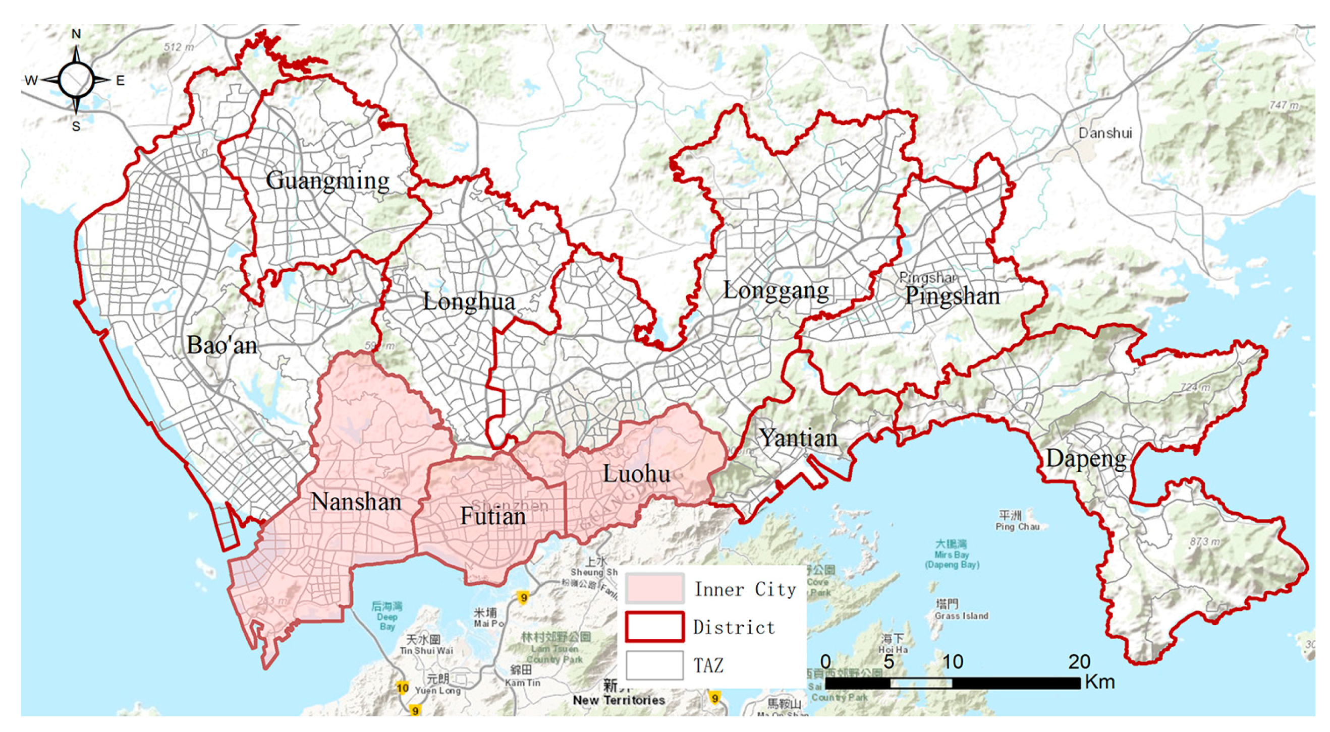
The TAZ was selected as the unit of spatial analysis, as it is suitable for investigating the spatial inequality in taxi services. In contrast to other commonly used spatial analysis units, such as district and sub-districts, the TAZ was more suitable because TAZs are delineated at a finer spatial scale that is based on the road network. In addition, TAZs are more appropriate than grid cells because TAZs contain similar land use types and economic and social attributes. As shown in Figure 1, there are 1067 TAZs in the city of Shenzhen. The pick-up and drop-off locations were aggregated based on the TAZ-level.

4. Methodology

This section presents the methods used to analyze spatial inequality in taxi services in the context of a subsidy war among e-hailing apps. A service rate is proposed to measure the quantity of taxi service in each TAZ. A Gini coefficient is introduced to assess the spatial inequality in taxi services. In this paper, a Theil index and its decomposition distinguish the contribution of the inner city and the outer city groups of TAZs, to compare these zones to the overall spatial inequality in taxi services.

4.1. Service Rate

Taxi services could be divided into two parts, arrival services and departure services. The arrival service and departure service of a TAZ can be depicted by the cumulative arrivals and departures within a TAZ, but the absolute number does not account for variation in the size or the total number of taxis active in the city during any particular period. A TAZ with a larger area has more arrival times and departure times than a smaller TAZ. Variations in the number of taxis and sampling days in each period also influence the quantity of taxi service. A measure called the service rate is proposed to control these factors. The service rate represents the arrival and departure times per car per unit area per day. The service rate is comprised of two parts, the arrival service rate (ASR) and the departure service rate (DSR) which are defined as follows:

$$AS{R}_i^p=\frac{{{\displaystyle \sum }}_{k=1}^n{o}_k{d}_i}{N^p{A}_i{T}^p}, DS{R}_i^p=\frac{{{\displaystyle \sum }}_{k=1}^n{o}_i{d}_k}{N^p{A}_i{T}^p}$$

(1)

where $AS{R}_i^p$ and $DS{R}_i^p$ denote the arrival service rate and departure service rate in TAZ $i$ in Period $p$. By constructing OD matrix, we can calculate the number of arrival times and departure times in each TAZ. In particular, $o_k{d}_i$ denotes the number of trips starting from TAZ $k$ and ending in TAZ $i$, and ${\displaystyle \sum }_{k=1}^n{o}_k{d}_i$ denotes the number of trips ending in TAZ $i$. Similarly, $o_i{d}_k$ denotes the number of trips starting from TAZ $i$ and ending in TAZ $k$, and ${\displaystyle \sum }_{k=1}^n{o}_i{d}_k$ denotes the number of trips starting from TAZ $i$. In addtion, $n$ denotes the total number of TAZs, which is equal to 1067 in this case, $N^p$ denotes the number of cars in Period $p$, and $A_i$ denotes the area of TAZ $i$. The value $T^p$ denotes the number of days in Period $p$, which in this study is equal to 12 weekdays or four weekend days.

4.2. Measurements of Spatial Inequality in Taxi Services

4.2.1. Gini Coefficient

The Gini coefficient was initially proposed as a means for estimating inequality in income distributions [12]. It also has been widely used to measure the inequality in public transport [3], health facilities [28], energy [29], and ecological footprints [30]. Here, a Gini coefficient is employed to measure the spatial inequality in taxi services. The formula for calculating the Gini coefficient is as follows:

$$G=1+\frac{1}{n}-\frac{2}{n^2\overline{x}}{\displaystyle \sum }_{i=1}^n\left(n-i+1\right)x_i$$

(2)

where $G$ denotes the Gini coefficient, $n$ denotes the number of TAZs, which is equal to 1067 in this case, and $\overline{x}$ denotes the mean value of service rate. The value $x_i$ denotes the service rate of TAZ $i$ in an ascending order. The range of the Gini coefficient is between 0 and 1, the higher the Gini coefficient, the more inequality.

4.2.2. Theil Index and Its Decomposition

The Theil index [31] is another widely used index to measure inequality. It has been widely used in several fields, such as energy intensity [32], energy consumption [33], regional development disparity [34], and energy efficiency [35]. Decomposability is a property of the Theil index which the Gini coefficient does not offer. The decomposition of the Theil index makes it possible to explore the contribution of different groups to overall inequality, as the spatial distribution of taxi services can vary significantly in different groups of TAZs, like the inner city and the outer city groups of TAZs; the higher the Theil index, the greater the level of inequality. The Theil index is calculated using the following formula:

$$T=\frac{1}{n}{\displaystyle \sum }_{i=1}^n\frac{x_i}{\overline{x}}\ln \frac{x_i}{\overline{x}}$$

(3)

where $T$ denotes the Theil index, other letters have identical meanings as the corresponding terms in Equation (1).

The Theil index can be decomposed into two parts, within-group and between-group inequality. In order to analyze the contribution of the inner city and the outer city groups of TAZs to the overall spatial inequality of taxi services, the TAZs in Shenzhen city were separated into inner city and outer city groups. The decomposition formula is shown as follows:

$$T=T_b+T_w={\displaystyle \sum }_{k=1}^K{y}_k\ln \left(\frac{y_k}{n_k/n}\right)+{\displaystyle \sum }_{k=1}^K{y}_k\left({\displaystyle \sum }_{i\in g_k}\frac{y_i}{y_k}\ln \frac{y_i/y_k}{1/n_k}\right)$$

(4)

where $T_b$ denotes the between-group inequality, $T_w$ denotes the within-group inequality, and $K$ is the number of groups, which is equal to two in this study. The value $n$ denotes the number of TAZs, $n_k$ is the number of TAZs in group $k$, and $g_k$ denotes the set of TAZs in group $k$. The term $y_i$ denotes the share of the service rate of TAZ $i$ in the total service rate, and $y_k$ denotes the share of sum of the service rate of group $k$ in the total service rate.

5. Results

5.1. The Changes of Service Rate in the Subsidy War

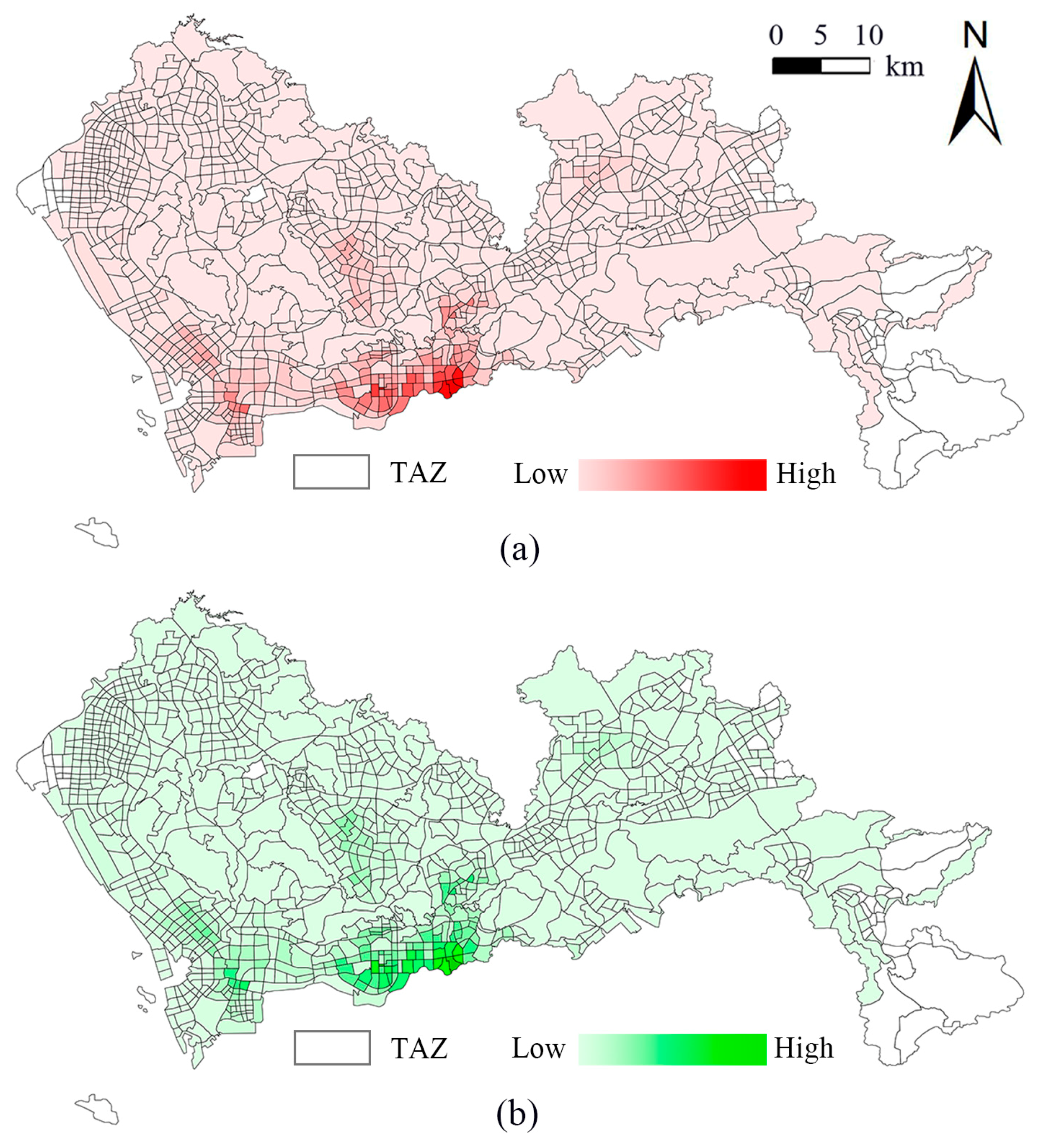
Figure 2 shows the spatial distribution of ASR and DSR on weekdays in Period 1 on TAZ-level, which indicates that the inner city has a higher value of service rate than the outer city at the aggregate level. In this paper, only the spatial distribution of service rate on weekdays in Period 1 are presented, since there was no significant difference in the spatial distribution of the service rate between the six periods or between weekdays and weekends.

In order to evaluate the changes of service rate on weekdays during the subsidy war, we calculated the mean service rate in three ways, the overall mean, the inner city mean, and the outer city mean, as shown in

Table 3. The overall mean of the ASR/DSR, the inner city mean of the ASR/DSR, and the outer city mean of the ASR/DSR on weekdays.

Period	ASR			DSR
	Overall Mean	Inner City Mean	Outer City Mean	Overall Mean	Inner City Mean	Outer City Mean
1	0.0466	0.1422 (70.04%)	0.0181 (29.96%)	0.0479	0.148 (70.90%)	0.0181 (29.10%)
2	0.0452	0.1396 (70.87%)	0.0171 (29.13%)	0.0465	0.1458 (72.01%)	0.0169 (27.99%)
3	0.0457	0.1354 (68.03%)	0.019 (31.97%)	0.0469	0.1402 (68.61%)	0.0191 (31.39%)
4	0.0454	0.139 (70.34%)	0.0175 (29.66%)	0.0465	0.1445 (71.31%)	0.0173 (28.69%)
5	0.0451	0.14 (71.21%)	0.0169 (28.79%)	0.0463	0.1452 (72.02%)	0.0168 (27.98%)
6	0.0461	0.1417 (70.64%)	0.0176 (29.36%)	0.0473	0.1468 (71.30%)	0.0176 (28.70%)

. Several conclusions can be drawn from Table 3:

(1)

The trends of change in the mean of ASR and DSR for the inner city are identical, which is the same as the trends of change in the mean of ASR and DSR for the outer city. However, they are different from the trends of change in the overall mean. The inner city mean decreased in Period 2 and decreased again in Period 3. This indicates that the considerable subsidy given to passengers and cabdrivers alike reduced the service rate in the inner city. In contrast, the service rate in the outer city increased significantly in Period 3 when the subsidy war was white-hot. This implies that some cabdrivers picked up and dropped off passengers in the outer city when they received high subsidies. When the subsidy given to passengers was reduced in Period 4, the inner city mean rose and the outer city mean decreased. When the subsidy on passengers was canceled, the inner city mean increased again and the outer city mean decreased again. Finally, when there was no subsidy for either passengers or cabdrivers, both the inner city and the outer city means increased.

(2)

The shares of the service rates in the inner city and the outer city in the total service rate are given in Table 3. The shares of the service rates in the inner city in Period 3 declined to 68.03% in the ASR and to 68.61% in the DSR. In addition, during Period 3, the shares of the service rates in the outer city rose to 31.97% in the ASR and to 31.39% in the DSR. This provides stronger evidence that some cabdrivers picked up and dropped off passengers in the outer city when they received larger subsidies.

Table 4. The overall mean of the ASR/DSR, the inner city mean of the ASR/DSR, and the outer city mean of the ASR/DSR on weekends.

Period	ASR			DSR
	Overall Mean	Inner City Mean	Outer City Mean	Overall Mean	Inner City Mean	Outer City Mean
1	0.0439	0.1281 (66.97%)	0.0188 (33.03%)	0.0453	0.1342 (68.03%)	0.0188 (31.97%)
2	0.0465	0.1415 (69.89%)	0.0182 (30.11%)	0.048	0.1487 (71.12%)	0.018 (28.88%)
3	0.0481	0.1404 (67.07%)	0.0205 (32.93%)	0.0495	0.1466 (68.01%)	0.0205 (31.99%)
4	0.0463	0.1374 (68.09%)	0.0192 (31.91%)	0.0476	0.1434 (69.11%)	0.0191 (30.89%)
5	0.0502	0.1502 (68.71%)	0.0204 (31.29%)	0.0516	0.1568 (69.72%)	0.0203 (30.28%)
6	0.0467	0.1396 (68.65%)	0.019 (31.35%)	0.0481	0.1459 (69.72%)	0.0189 (30.28%)

shows the overall mean of service rate, the inner city mean of service rate, and the outer city mean of service rate on weekends. The trend of change on weekends in Table 4 shows clear differences in comparison with the mean service rates for weekdays as shown in Table 3. For example, the trends of change in the mean of ASR and DSR for the inner city in Table 4 are both “increase-decrease-decrease-increase-decrease” and the trends of change in the mean of the ASR and DSR for the outer city are both “decrease-increase-decrease-increase-decrease”. Table 4 also demonstrates that when the subsidy war had just begun in Period 2, the share of the inner city as a share of the total service rate increased dramatically while the share of the outer city declined. This suggests that the subsidy war motivated cabdrivers to pick up and drop off more passengers in the inner city on weekends. Furthermore, when the subsidy war was white-hot in Period 3, the inner city as a share of the total service rate declined almost to the level found in Period 1, implying that the substantial subsidy offered to cabdrivers at that time motivated them to pick up and drop off more passengers in the outer city on weekends.

5.2. Spatial Inequality in Taxi Services

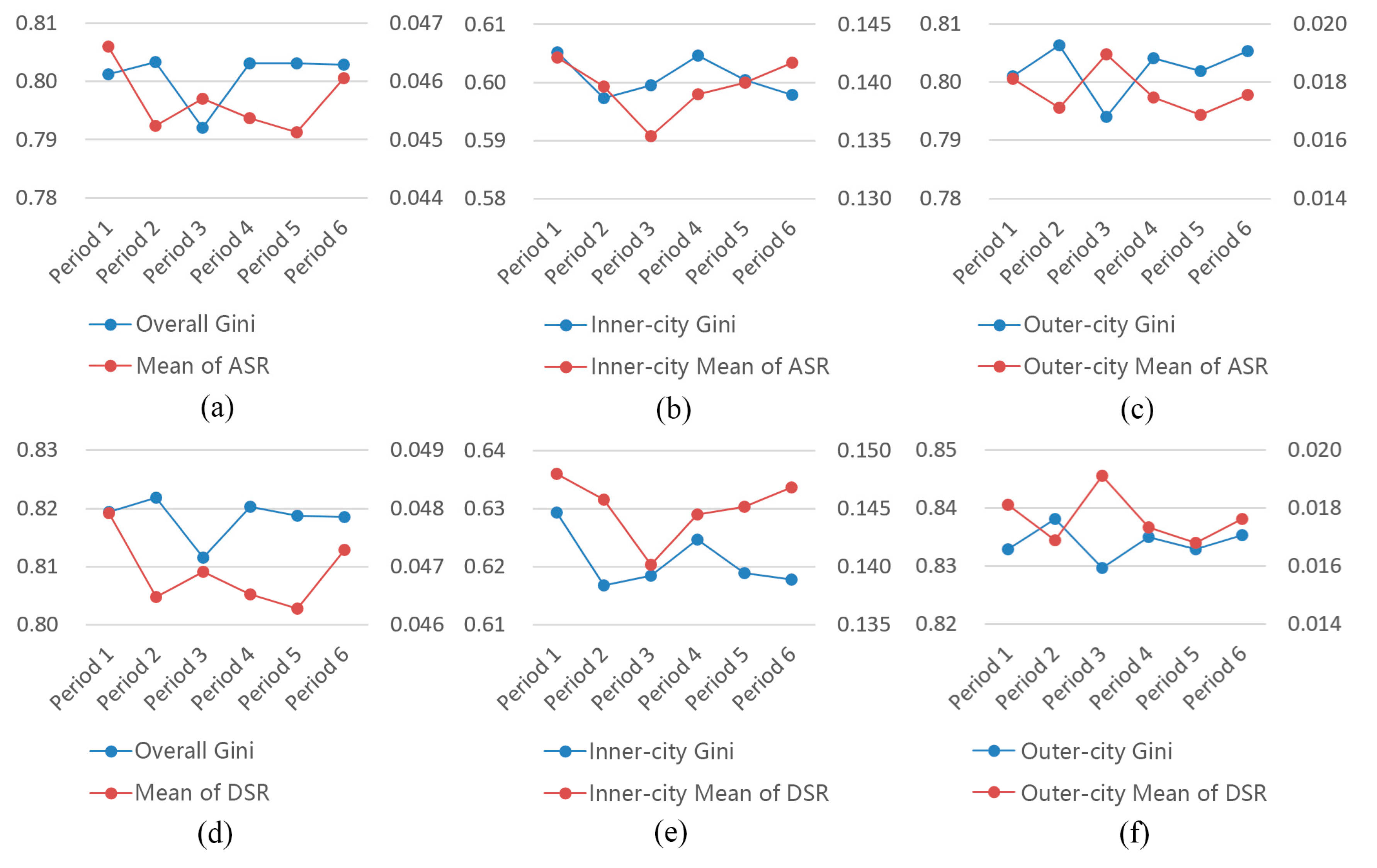
Figure 3 shows the changes of Gini coefficient and mean of service rate on weekdays during the subsidy war. The TAZs were divided into inner city and outer city groups. Gini coefficients were calculated in three ways, the overall Gini, the inner city Gini, and the outer city Gini, as shown in Figure 3.

The overall Gini coefficient of ASR ranges from 0.79 to 0.81, which indicates that Shenzhen City has relatively high spatial inequality in taxi services. The Gini coefficient for the ASR of the inner city TAZs ranges from 0.59 to 0.61 and the Gini coefficient of the outer city TAZs ranges from 0.79 to 0.81. This indicates that the outer city has greater spatial inequality in the ASR than the inner city. This conclusion also fits into the spatial inequality in the DSR. The changes in the Gini coefficient during the subsidy war are summarized in detail as follows:

(1)

Comparing Period 1 to Period 2, the overall spatial inequality in service rate is strengthened and so does the spatial inequality of the outer city. However, the spatial inequality of the inner city is weakened. The small subsidies given by the two companies when the subsidy war had just begun aggravated inequality in the outer city, but alleviated inequality in the inner city. Comparing Period 2 to Period 3, overall inequality was weakened significantly, as was inequality in the outer city, but the inequality of the inner city increased slightly. This indicates that the substantial subsidy alleviated the inequality of outer city effectively but had little influence on the inequality of the inner city. Comparing Period 3 to Period 4, the overall inequality rebounded to its original level and the inequalities of inner city and outer city were both aggravated. Thus, when the subsidy given to passengers was reduced, the inequality of taxi services was aggravated. Comparing Period 4 to Period 5, the overall inequality was almost unchanged and the inequalities in the inner city and outer city were both lower, this indicates that when the subsidy to passengers was cancelled, the inequality of taxi service of inner city and outer city was alleviated. Comparing Period 5 to Period 6, the overall inequality was almost unchanged, the inequality of inner city was reduced, and the inequality of outer city increased.

(2)

The lowest value of the Gini coefficient for the overall city occurred during Period 3 when the mean value of service rate was relatively low compared with its original level in Period 1. In the case of the inner city, the most equitable situation occurred in Period 2 when the mean value of service rate was relatively low as compared with its original level in Period 1. Thus, the inner city had the most equitable taxi services in Period 2; however, each TAZ had a relatively low value for the service rate relative to Period 1. For the outer city, the most equitable situation occurred in Period 3, when the mean value of service rate arrived at the peak.

(3)

A comparison of the Gini coefficients and mean values of service rate in Period 1 and Period 6, shows that the overall inequality was nearly unchanged at the beginning and end of the subsidy war, the inequality of inner city was alleviated a little, and inequality in outer city was aggravated slightly. Thus, the subsidy war alleviated the spatial inequality in taxi services in the inner city but aggravated it in the outer city.

Figure 4 shows the changes in the Gini coefficients and mean of the service rates on weekends during the subsidy war. The trend of change in the Gini coefficient on weekends display several differences with the values for weekdays, as presented in Figure 3. The trend of change in the Gini coefficient for inner city TAZs on weekends was “decrease-decrease-increase-decrease-increase”, which is different from the pattern on weekdays. The trend of change in the Gini coefficient for the outer city on weekends was “increase-decrease-increase-increase-decrease”, which is also different from the pattern on weekdays. The lowest Gini coefficient value for the overall city occurred during Period 3 when the mean value of the service rate was high, relative to its original level in Period 1. For the inner city, the lowest Gini coefficient occurred in Period 3 when the mean value of service rate was relatively high. For the outer city, the lowest Gini coefficient also occurred in Period 3 when the mean value of service rate was the highest.

5.3. Between-Group and within-Group Spatial Inequalities in Taxi Services

When dividing the TAZs into inner city and the outer city groups, the Theil index decomposition method distinguishes the contribution of TAZs in the inner and the outer city to the overall spatial inequality of taxi services.

Table 5. The Theil index and its decomposition of the service rate on weekdays.

Period	ASR			DSR
	Theil Index	Between-Group Inequality	Within-Group Inequality	Theil Index	Between-Group Inequality	Within-Group Inequality
1	1.3450	0.4896 (36.40%)	0.8554 (63.60%)	1.4313	0.4887 (34.14%)	0.9426 (65.86%)
2	1.3554	0.5048 (37.25%)	0.8506 (62.75%)	1.4436	0.5206 (36.06%)	0.9230 (63.94%)
3	1.2970	0.4478 (34.53%)	0.8492 (65.47%)	1.3858	0.4491 (32.40%)	0.9367 (67.60%)
4	1.3550	0.4969 (36.67%)	0.8581 (63.33%)	1.4369	0.5029 (35.00%)	0.9341 (65.00%)
5	1.3552	0.5132 (37.87%)	0.8420 (62.13%)	1.4267	0.5120 (35.89%)	0.9146 (64.11%)
6	1.3538	0.5061 (37.38%)	0.8477 (62.62%)	1.4257	0.5012 (35.15%)	0.9245 (64.84%)

shows the results of the Theil index and its decomposition of the service rate on weekdays. As shown, the within-group inequality contributed more than 60% of the total inequality, whereas between-group inequality accounted for less than 40%. The primary contributor to the overall spatial inequality in taxi services was the within-group inequality in taxi services rather than the between-group inequality. Period 3 has the highest contribution rate to within-group inequality, which indicates that a large subsidy increased the rate of contributions from within-group inequality to the overall service inequality.

The Theil index and its decomposition of service rate results for weekends are shown in

Table 6. The Theil index and its decomposition of the service rate on weekends.

Period	ASR			DSR
	Theil Index	Between-Group Inequality	Within-Group Inequality	Theil Index	Between-Group Inequality	Within-Group Inequality
1	1.2910	0.4198 (32.52%)	0.8712 (67.48%)	1.3651	0.4184 (30.65%)	0.9468 (69.35%)
2	1.3399	0.4754 (35.48%)	0.8646 (64.52%)	1.4140	0.4881 (34.52%)	0.9259 (65.48%)
3	1.2602	0.4212 (33.42%)	0.8390 (66.58%)	1.3369	0.4250 (31.79%)	0.9119 (68.21%)
4	1.2997	0.4440 (34.16%)	0.8557 (65.84%)	1.3658	0.4473 (32.75%)	0.9185 (67.25%)
5	1.3105	0.4521 (34.50%)	0.8584 (65.50%)	1.3861	0.4692 (33.85%)	0.9169 (66.15%)
6	1.3210	0.4571 (34.60%)	0.8640 (65.40%)	1.3850	0.4616 (33.33%)	0.9233 (66.67%)

. Several conclusions can be drawn when comparing with the values on weekdays as given in Table 5. The contribution rates of within-group inequality on weekends are higher than the values on weekdays during the same periods. This indicates that the inequality within the inner city and the inequality within the outer city contributed more to the overall inequality on weekends as compared to the same values for weekdays. The highest contribution rate of within-group inequality occurred in Period 1 on weekends.

5.4. The Spatial Inequality in the Service Rate Change

The service rate change for each TAZ was obtained by subtracting the service rate in the current period from the service rate in the next period. The spatial inequality in service rate change was analyzed with the Gini coefficient, and the Theil index and its decomposition as measures of similarity. Accordingly, Periods 1–2, 2–3, 3–4, 4–5, and 5–6 denote pairs of neighboring periods in the subsidy war.

Table 7. The overall mean, the inner city mean, and the outer city mean of increased and decreased service rate on weekdays between each pair of neighboring periods.

Inter Period	Increased ASR			Decreased ASR
	Overall Mean	Inner City Mean	Outer City Mean	Overall Mean	Inner City Mean	Outer City Mean
1–2	0.004481	0.010208	0.001891	0.003904	0.011181	0.002109
		(70.93%)	(29.07%)		(56.66%)	(43.34%)
2–3	0.003411	0.007572	0.002725	0.008432	0.014161	0.002525
		(31.40%)	(68.60%)		(85.25%)	(14.75%)
3–4	0.004414	0.008203	0.000518	0.002096	0.003129	0.001942
		(94.22%)	(5.78%)		(19.31%)	(80.69%)
4–5	0.001755	0.004405	0.000466	0.001991	0.005710	0.001348
		(82.14%)	(17.86%)		(42.28%)	(57.72%)
5–6	0.002448	0.004922	0.001629	0.001058	0.003293	0.000471
		(50.02%)	(49.98%)		(64.73%)	(35.27%)
Inter Period	Increased DSR			Decreased DSR
	Overall Mean	Inner City Mean	Outer City Mean	Overall Mean	Inner City Mean	Outer City Mean
1–2	0.002676	0.006810	0.000736	0.004424	0.013651	0.002434
		(81.27%)	(18.73%)		(54.73%)	(45.27%)
2–3	0.003454	0.007117	0.002964	0.007080	0.012691	0.000788
		(24.34%)	(75.66%)		(94.75%)	(5.25%)
3–4	0.004623	0.008246	0.000317	0.002456	0.003645	0.002309
		(96.86%)	(3.14%)		(16.29%)	(83.71%)
4–5	0.001775	0.008246	0.000640	0.002136	0.003645	0.001367
		(76.41%)	(23.59%)		(44.70%)	(55.30%)
5–6	0.002609	0.005363	0.001753	0.001142	0.003645	0.000419
		(48.74%)	(51.26%)		(71.89%)	(28.11%)

shows the overall mean of the increased and decreased service rate, the mean of the inner-city increased and decreased service rate, and the mean of the increased and decreased outer-city service rate on weekdays between each pair of neighboring periods. Several conclusions can be drawn from Table 7:

(1)

The mean values of the service rate change in the inner city TAZs was always larger than the mean values of the service rate change in the outer city, because as discussed in Section 5.1, the inner city has a larger service rate value than the outer city at the aggregate level. Thus, the mean of the service rate change in the inner city was also larger than the mean of the service rate change in the outer city.

(2)

Increases and decreases in share of the ASR and DSR values in these neighboring periods show similar trends of change. For example, the increased ASR of the inner-city TAZs accounted for 70.93% of the total increase in ASR in Period 1–2 and the increased DSR of inner-city TAZs accounted for 81.27% of the total increase in the DSR in Period 1–2. This indicates that the inner city contributed to the majority of the increased service rate. In Period 2–3, the increased ASR and DSR values of inner city TAZs accounted for 31.40% and 24.36% of the total increase of the ASR ad DSR, respectively, which implies that the inner city has a lower increased service rate. Moreover, in Period 3–4, the increased ASR and DSR values of inner city TAZs accounted for about 95% of the total increase in ASR and DSR, which suggests that nearly the entire increased service rate happened in the inner city. In Period 4–5, the shares of the increased ASR and DSR values of inner city TAZs decreased to 82.14% and 76.41%, respectively. Finally, the shares of the increased ASR and DSR of inner city decrease again to 50.02% and 48.74% in Period 5–6. The overall mean, the inner-city mean, and the outer-city mean of increased and decreased service rate on weekends were calculated for each pair of neighboring periods. These results also show that the mean values of the service rate change in inner city TAZs were always larger than the of the values for outer city TAZs. The sharpest differences in the shares of the changed service rate between weekdays and weekends are the shares of decreased service rates in Period 1–2 and Period 3–4. In particular, the shares of the decreased ASR and DSR values for inner city TAZs reach 12.18% and 6.91% in Period 1–2, which indicates that the major decreases in service rates occurred in outer city rather than inner city TAZs. In Period 3–4, the shares of the decreased ASR and DSR values for inner city TAZs reached 53.23% and 50.50%, respectively, which indicates that about half of the decreased service rate occurred in inner city TAZs.

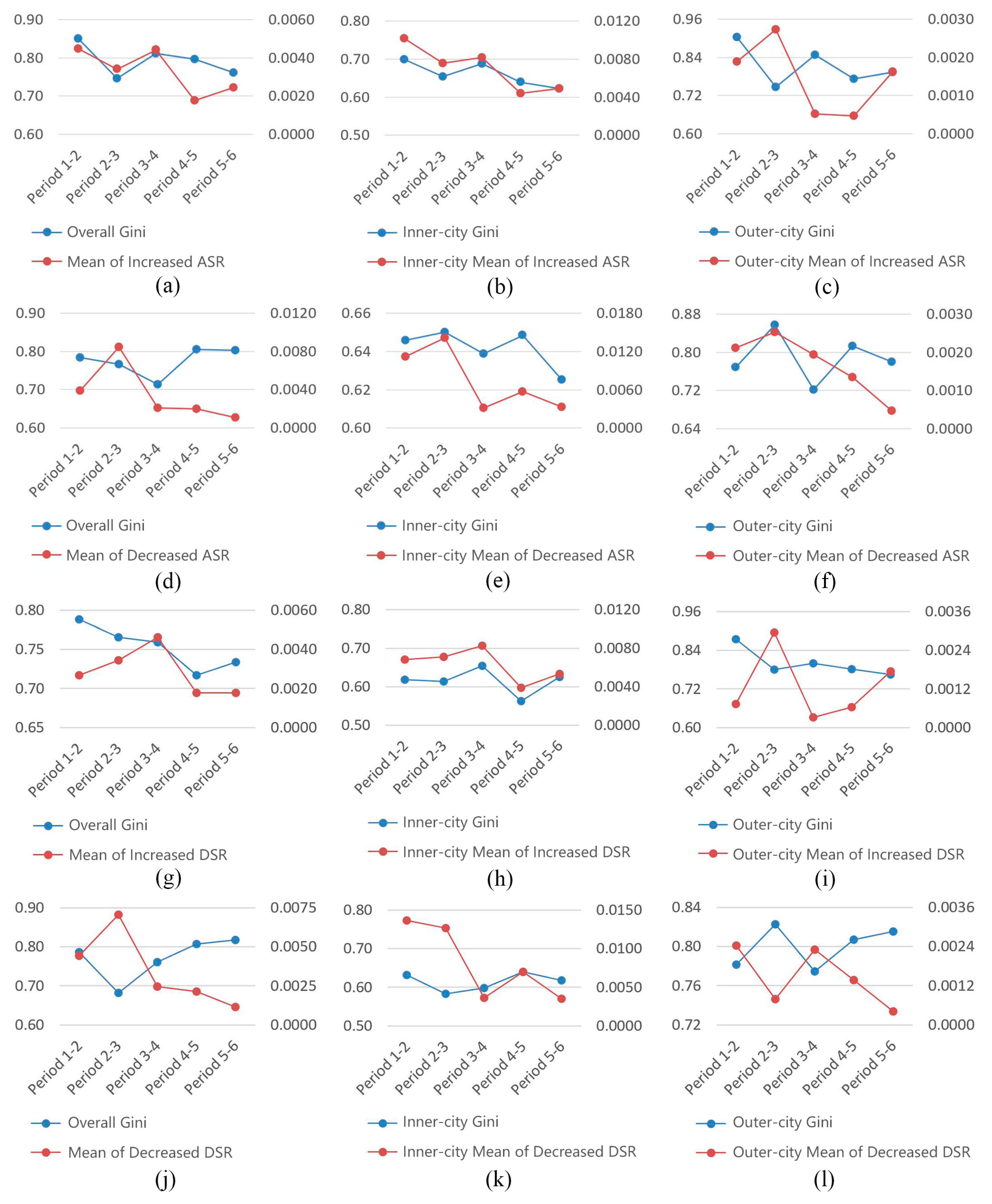
Figure 5 shows that the Gini coefficients of inner city TAZs were always smaller than the Gini coefficients of outer city TAZs, which indicates that the inner city is more equitable than the outer city in service rate change. Taking the increased ASR in Period 2–3 as an example, when the two companies increased the subsidy, the overall Gini coefficient for the increased ASR declined while the mean of the increased ASR was at the medium level, when compared with other periods. The Gini coefficient of the increased ASR in inner city TAZs present a similar, but declining trend and the mean increased ASR for inner city TAZs was also at the medium level. In addition, the Gini coefficient of the increased ASR of the outer city TAZs declined to its lowest level compared with other periods, while the mean of the increased ASR for outer-city TAZs was at the highest level. This indicates that in Period 2–3 the outer city TAZs had the highest increased ASR and service rate reached the most equitable situation. Furthermore, the overall, the inner city, and the outer-city Gini coefficients for increased ASR values declined when the two companies reduced the subsidy to passengers in Period 3–4. Moreover, the mean increased ASR for inner city TAZs rose slightly while the mean increased ASR for outer-city TAZs dropped dramatically. In Period 4–5, the overall, the inner city, and both the outer-city Gini coefficients and their mean values of increased ASR also decreased. In period 5–6, the overall and the inner-city TAZ Gini coefficients both declined while the Gini coefficient of outer city TAZs increased a little. In addition, mean values of increased ASR for the overall, the inner-city, and the outer-city TAZs rose in Period 5–6.

Table 8. The Theil index and its decomposition of the service rate change on weekdays.

Inter Period	Increased ASR			Increased DSR
	Theil Index	Between-Group Inequality	Within-Group Inequality	Theil Index	Between-Group Inequality	Within-Group Inequality
1–2	1.6498	0.3333 (20.20%)	1.3165 (79.80%)	1.2648	0.3593 (28.41%)	0.9055 (71.59%)
2–3	1.0965	0.0965 (8.80%)	1.0000 (91.20%)	1.1596	0.0699 (6.02%)	1.0898 (93.98%)
3–4	1.4184	0.4599 (32.42%)	0.9585 (67.58%)	1.1385	0.3471 (30.49%)	0.7914 (69.51%)
4–5	1.4871	0.5190 (34.90%)	0.9681 (65.10%)	0.9748	0.2773 (28.44%)	0.6975 (71.56%)
5–6	1.1571	0.1457 (12.59%)	1.0114 (87.41%)	1.0468	0.0999 (9.55%)	0.9468 (90.45%)
Inter Period	Decreased ASR			Decreased DSR
	Theil Index	Between-Group Inequality	Within-Group Inequality	Theil Index	Between-Group Inequality	Within-Group Inequality
1–2	1.2755	0.3294 (25.83%)	0.9461 (74.17%)	1.2750	0.3234 (25.36%)	0.9516 (74.64%)
2–3	1.1675	0.2642 (22.63%)	0.9033 (77.37%)	0.8634	0.2235 (25.89%)	0.6399 (74.11%)
3–4	0.9711	0.0160 (1.65%)	0.9551 (98.35%)	1.1614	0.0107 (0.92%)	1.1507 (99.08%)
4–5	1.3825	0.2203 (15.93%)	1.1622 (84.07%)	1.3606	0.2871 (21.10%)	1.0735 (78.90%)
5–6	1.3863	0.4498 (32.45%)	0.9364 (67.55%)	1.4148	0.5396 (38.14%)	0.8752 (61.86%)

shows the Theil index and its decomposition results for the service rate change on weekdays. The within-group inequality always contributed more to the overall spatial inequality, which indicates that the primary contributor of the spatial inequality in the service rate change was the within-group inequality. This conclusion is consistent with the Theil index and the decomposition results for the service rate change on weekends, thus we only present the results for weekdays.

6. Conclusions

The research presented in this paper investigated the spatial inequality of taxi services in the context of the 2014 subsidy war among e-hailing apps in Shenzhen, China. The subsidy war was divided into six sub-periods based on the amount of subsidies passengers and cabdrivers obtained in different periods. A new service rate indicator is proposed to measure the quantity of taxi services in TAZs. A Gini coefficient is used to assess the spatial inequality in taxi services. The Theil index and its decomposition were used to analyze the contribution of grouped inner city and outer city TAZs to overall spatial inequality. The main findings are summarized as follows:

First, the subsidy war finally alleviated the spatial inequality in taxi services of the inner city while aggravated the inequality of the outer city. In addition, when dividing the entire TAZs into the inner and outer city groups of TAZs, it shows that the outer city TAZs had greater inequality in taxi services than inner city TAZs.

Second, the primary contributor to the overall inequality in taxi services was inequality within, rather than between, the inner and outer city. In addition, the highest contribution rate of within-group inequality occurred in Period 3 on weekdays, which indicates that a large subsidy increased the contribution rate of within-group inequality. On weekends, the highest contribution rate from within-group inequality occurred in Period 1 when the subsidy war had not yet begun.

Third, the mean values for the changed service rates in the inner city were always larger than the outer city TAZs, and the inner city TAZs had a more equitable changed service rate than the outer city TAZS. Moreover, the primary contributor of the overall inequality in the changed service rate was inequality within the inner and outer city.

It is also important to highlight certain aspects of our data that might introduce some potential bias in this study. Taxi demand is strongly related to the distribution of the population. However, taxi trajectory data only covers the actual number of taxi services other than the real taxi demands. For example, people who request taxi services but fail to obtain these services are not recorded in taxi trajectory data. With this limitation, we only focus on the spatial inequality in the actual number of taxi services. Future studies could incorporate population data and taxi order data in e-hailing apps to study spatial inequality in taxi demands.

References

- Murray, A.T.; Davis, R. Equity in Regional Service Provision. J. Reg. Sci. 2001, 41, 557–600. [Google Scholar] [CrossRef]
- Wu, B.M.; Hine, J.P. A PTAL approach to measuring changes in bus service accessibility. Transp. Policy 2003, 10, 307–320. [Google Scholar] [CrossRef]
- Delbosc, A.; Currie, G. Using Lorenz curves to assess public transport equity. J. Transp. Geogr. 2011, 19, 1252–1259. [Google Scholar] [CrossRef]
- Litman, T. Evaluating Transportation Equity: Guidance for Incorporating Distributional Impacts in Transportation Planning. World Transp. Policy Pract. 2002, 8, 50–65. [Google Scholar]
- Foth, N.; Manaugh, K.; Elgeneidy, A.M. Toward Equitable Transit: Examining Transit Accessibility and Social Need in Toronto, Canada, 1996–2006. In Proceedings of the Transportation Research Board 92nd Annual Meeting, Washington, DC, USA, 13–17 January 2013; pp. 1–10. [Google Scholar]
- Currie, G. Gap analysis of public transport needs: Measuring spatial distribution of public transport needs and identifying gaps in the quality of public transport provision. Transp. Res. Rec. 2004, 1895, 137–146. [Google Scholar] [CrossRef]
- Currie, G.; Wallis, I. Determining Priorities for Passenger Transport Funding: The Needs Assessment Approach. In Proceedings of the Papers of the Australasian Transport Research Forum, Canberra, Australia, 7–9 October 1992. [Google Scholar]
- Qian, X.; Ukkusuri, S.V. Spatial variation of the urban taxi ridership using GPS data. Appl. Geogr. 2015, 59, 31–42. [Google Scholar] [CrossRef]
- Sootoo Institute. China E-Hailing Service Market Research Report in 2017. Available online: http://www.sootoo.com/content/675157.shtml (accessed on 23 March 2018).
- Delmelle, E.C.; Casas, I. Evaluating the spatial equity of bus rapid transit-based accessibility patterns in a developing country: The case of Cali, Colombia. Transp. Policy 2012, 20, 36–46. [Google Scholar] [CrossRef]
- Lorenz, M.O. Methods of Measuring the Concentration of Wealth. Publ. Am. Stat. Assoc. 1905, 9, 209–219. [Google Scholar] [CrossRef]
- Gini, C. Variabilità e Mutabilità; Pizetti, E., Salvemini, T., Eds.; Libreria Eredi Virgilio Veschi: Rome, Italy, 1912; Volume 1. [Google Scholar]
- Bhandari, K.; Kato, H.; Hayashi, Y. Economic and Equity Evaluation of Delhi Metro. Int. J. Urban Sci. 2009, 13, 187–203. [Google Scholar] [CrossRef]
- Jang, S.; An, Y.; Yi, C.; Lee, S. Assessing the spatial equity of Seoul’s public transportation using the Gini coefficient based on its accessibility. Int. J. Urban Sci. 2017, 21, 91–107. [Google Scholar] [CrossRef]
- Cao, X.; Chen, H.; Liang, F.; Wang, W. Measurement and Spatial Differentiation Characteristics of Transit Equity: A Case Study of Guangzhou, China. Sustainability 2018, 10, 1069. [Google Scholar] [CrossRef]
- Noulas, A.; Salnikov, V.; Hristova, D.; Mascolo, C.; Lambiotte, R. Developing and Deploying a Taxi Price Comparison Mobile App in the Wild: Insights and Challenges. arXiv, 2017; arXiv:1701.04208. [Google Scholar]
- Salnikov, V.; Lambiotte, R.; Noulas, A.; Mascolo, C. OpenStreetCab: Exploiting Taxi Mobility Patterns in New York City to Reduce Commuter Costs. arXiv, 2015; arXiv:1503.03021. [Google Scholar]
- Harding, S.; Kandlikar, M.; Gulati, S. Taxi apps, regulation, and the market for taxi journeys. Transp. Res. Part A Policy Pract. 2016, 88, 15–25. [Google Scholar] [CrossRef]
- Chen, L.; Mislove, A.; Wilson, C. Peeking Beneath the Hood of Uber. In Proceedings of the Internet Measurement Conference, Tokyo, Japan, 28–30 October 2015; pp. 495–508. [Google Scholar]
- Noulas, A.; Salnikov, V.; Lambiotte, R.; Mascolo, C. Mining open datasets for transparency in taxi transport in metropolitan environments. EPJ Data Sci. 2015, 4, 1–19. [Google Scholar] [CrossRef]
- He, F.; Shen, Z.-J.M. Modeling taxi services with smartphone-based e-hailing applications. Transp. Res. Part C Emerg. Technol. 2015, 58, 93–106. [Google Scholar] [CrossRef]
- Qian, X.; Ukkusuri, S.V. Taxi market equilibrium with third-party hailing service. Transp. Res. Part B Methodol. 2017, 100, 43–63. [Google Scholar] [CrossRef]
- Zha, L.; Yin, Y.; Du, Y. Surge Pricing and Labor Supply in the Ride-Sourcing Market. Transp. Res. Procedia 2017, 23, 2–21. [Google Scholar] [CrossRef]
- Wang, X.; He, F.; Yang, H.; Oliver Gao, H. Pricing strategies for a taxi-hailing platform. Transp. Res. Part E Logist. Transp. Rev. 2016, 93, 212–231. [Google Scholar] [CrossRef]
- Wen, J.; Zou, M.; Ma, Y.; Luo, H. Evaluating the Influence of Taxi Subsidy Programs on Mitigating Difficulty Getting a Taxi in Basis of Taxi Empty-loaded Rate. Int. J. Stat. Probab. 2017, 6, 9–20. [Google Scholar] [CrossRef]
- Leng, B.; Du, H.; Wang, J.; Li, L.; Xiong, Z. Analysis of Taxi Drivers’ Behaviors Within a Battle Between Two Taxi Apps. IEEE Trans. Intell. Transp. Syst. 2016, 17, 296–300. [Google Scholar] [CrossRef]
- Su, R.; Fang, Z.; Luo, N.; Zhu, J. Understanding the Dynamics of the Pick-Up and Drop-Off Locations of Taxicabs in the Context of a Subsidy War among E-Hailing Apps. Sustainability 2018, 10, 1256. [Google Scholar] [CrossRef]
- Theodorakis, P.N.; Mantzavinis, G.D.; Rrumbullaku, L.; Lionis, C.; Trell, E. Measuring health inequalities in Albania: A focus on the distribution of general practitioners. Hum. Resour. Health 2006, 4, 5. [Google Scholar] [CrossRef] [PubMed]
- Jacobson, A.; Milman, A.D.; Kammen, D.M. Letting the (energy) Gini out of the bottle: Lorenz curves of cumulative electricity consumption and Gini coefficients as metrics of energy distribution and equity. Energy Policy 2005, 33, 1825–1832. [Google Scholar] [CrossRef]
- Chen, D.; Ma, X.; Mu, H.; Li, P. The inequality of natural resources consumption and its relationship with the social development level based on the ecological footprint and the HDI. J. Environ. Assess. Policy Manag. 2010, 12, 69–86. [Google Scholar] [CrossRef]
- Theil, H. Economics and Information Theory; North-Holland Publishing Company: Amsterdam, The Netherlands, 1967. [Google Scholar]
- Alcantara, V.; Duro, J.A. Inequality of energy intensities across OECD countries: A note. Energy Policy 2004, 32, 1257–1260. [Google Scholar] [CrossRef]
- Zhang, L.; Yang, Z.; Liang, J.; Cai, Y. Spatial Variation and Distribution of Urban Energy Consumptions from Cities in China. Energies 2010, 4, 26–38. [Google Scholar] [CrossRef] [Green Version]
- Rayevneva, O.V.; Bobkova, O.Y. Identifying sources of development disparities of Ukraine’s regions basing on decomposition of theil index. Actual Probl. Econ. 2012, 2, 200–210. [Google Scholar]
- Feng, C.; Lu, B.; Xu, Z. A weighted Gini coefficient and Theil index-based approach for estimating the spatial disparity in energy efficiency in China. Int. J. Glob. Energy Issues 2016, 39, 4–17. [Google Scholar] [CrossRef]
Figure 1.
The administrative districts and traffic analysis zones (TAZs) of Shenzhen city.
Figure 2.
The spatial distribution of ASR (a) and DSR (b) on weekdays in Period 1.
Figure 3.
The changes of Gini coefficient and the changes of the mean of service rate on weekdays during the subsidy war. Specifically, they are the overall changes of the Gini coefficient and mean of ASR (a), the changes of the inner-city Gini coefficient and the inner-city mean of ASR (b), the changes of outer-city Gini coefficient and the outer-city mean of ASR (c), the overall changes of the Gini coefficient and the mean of DSR (d), the changes of inner-city Gini coefficient and the inner-city mean of DSR (e), and the changes of the outer-city Gini coefficient and the outer-city mean of DSR (f).
Figure 4.
The changes of the Gini coefficient and the changes of the mean of service rate on weekends during the subsidy war. Specifically, they are the overall changes of the Gini coefficient and mean of ASR (a), the changes of the inner-city Gini coefficient and the inner-city mean of ASR (b), the changes of the outer-city Gini coefficient and the outer-city mean of ASR (c), the overall changes of the Gini coefficient and the mean of DSR (d), the changes of the inner-city Gini coefficient and the inner-city mean of DSR (e), and the changes of the outer-city Gini coefficient and the outer-city mean of DSR (f).
Figure 5.
The changes of the Gini coefficient and the changes of the mean of the service rate change on weekdays between each pair of neighboring periods. Specifically, they are the overall changes of the Gini coefficient and the mean of increased ASR (a), the changes of the inner-city Gini coefficient and the inner-city mean of increased ASR (b), the changes of the outer-city Gini coefficient and the outer-city mean of increased ASR (c), the overall changes of the Gini coefficient and the mean of decreased ASR (d), the changes of the inner-city Gini coefficient and the inner-city mean of decreased ASR (e), the changes of the outer-city Gini coefficient and the outer-city mean of decreased ASR (f), the overall changes of the Gini coefficient and the mean of increased DSR (g), the changes of the inner-city Gini coefficient and the inner-city mean of increased DSR (h), the changes of the outer-city Gini coefficient and the outer-city mean of increased DSR (i), the overall changes of the Gini coefficient and the mean of decreased DSR (j), the changes of the inner-city Gini coefficient and the inner-city mean of decreased DSR (k), and the changes of the outer-city Gini coefficient and the outer-city mean of decreased DSR (l).