The Influence of the Shape and Size of the Cell on Developing Military Passability Maps

Abstract

The necessity to divide the analysed area into basic elements, regardless of the administrative division (cells or pixels, also called primary fields), and use them to prepare thematic maps emerged as early as by the end of the 19th century. The automation of map development processes brought a new approach to the function of cells, which made them a carrier that facilitates information processing, and presenting the results of analyses in the form of studies that very often function only in spatial information systems or on the Internet. Cells are currently used to conduct a series of advanced spatial analyses in practically all areas of application. The aim of the presented research was to analyse the influence of the shape and size of cells on the terrain classification results for the purposes of developing military passability maps. The research used the automatic terrain classification method, based on calculating the index of passability, calculated for cells of square, triangular, and hexagonal shapes and of different sizes, ranging from 100 m to 10,000 m. Indices of passability were determined basing on parameters derived from land cover elements that exist in the area of each of the adopted cells. Because of the fact that passability maps are mainly developed for military purposes, the study used a standardised vector spatial database—VMap Level 2. The studies have demonstrated that, if the surface areas of cells are identical, their shapes do not have a significant influence on the resulting passability map. The authors have also determined the sizes of cells that should be adopted for developing passability maps on various levels of accuracy, and, as a consequence, for being used on various levels of command of military troops.

1. Introduction

Frequent changes in the delimitations of the administrative division, which constitute a kind of natural reference units for spatial information, as well as the lack of such divisions on a higher level of detail, resulted in the need to use such reference units that are free from such disadvantages. One of the ways to solve these problems was to divide the area of interest into elementary units organized in regular cells, treated as a spatial reference field. Such a system is independent from the administrative division and is more relevant for terrain analysis because it is able to analyse the area according to geographical boundaries instead of administrative ones, as well as to analyse the terrain on various levels of detailedness. Cartographers have seen the necessity to use cells to generate thematic maps for a long time. The first publications that discussed the issue of dividing the country into regular cells appeared as early as at the end of the 19th century in Germany [1].

The automation of map generating processes brought a new approach to the function of spatial reference fields. These fields, previously treated only as one of the ways of spatial identification and recording of information, suddenly started to play an important role as information carriers. Even more, they became a carrier whose structure provided a basis for facilitating information processing and presenting information in the form of cartographic thematic studies. These studies were less and less frequently used outside the system in printed form. To the contrary, they began to function only in spatial information systems or on the Internet. Such maps are prepared as a result of a series of spatial analyses [2], and these transformations result in generating a thematic layer that represents the final outcome of the conducted analyses. As a result of the development of information technology systems, cells started to be used to refer information obtained from increasingly advanced analyses. Thus, the scope of their application is practically unlimited. They are used for analyses of demographic phenomena and land management [3,4], land development [5], or hydrological simulations. The latter may focus on land topography, soil cover [6], or vegetation [7], and are just a few of the numerous examples of multi-aspect analyses conducted with the use of cells.

With the popularisation of the Internet, interactive and dynamic maps have also become increasingly popular and desirable [8]. Internet maps are also generated based on the results of the analysis of data collected in a cell system and supplemented by vector data. This is how the map of potential damages caused by earthquakes and the map of existing deciduous forests in European Union Member States were created [9]. Interactive maps function freely as desktop applications or on websites. Their advantage is the fact that users may not only interfere with the type of displayed information, but also change the way in which it is presented. What makes the data gathered in cells even more interesting, is the fact that it is possible to change the resolution of the cell system [10], and thus to determine the influence of the size of cells on the level of detail of the visualisation of a specific phenomenon and to compare phenomena on various levels of detailedness. The most popular studies on this topic are the works on the selection of the cells resolution for the purposes of a digital terrain model [11,12,13,14]. From the cartographic point of view, research on the principles for selecting the appropriate resolution of the cells of the resulting maps depending on input data properties is essential, while linking them to the scale of the resulting map is particularly important [15,16,17].

Considering the above, the authors started research on the application of cells in the development of passability maps. The objective of these cartographic studies commonly generated by military forces is to support the planning process. The aim of passability maps is to determine the conditions of cross country movement of own and enemy armed forces off-road and in any meteorological conditions. In practice, such analyses are performed in military units by experienced officers from reconnaissance cells, and they involve manually marking impassable (NO GO) and low-passability (SLOW GO) areas, basing on the analysis of cartographic materials. Unmarked areas are treated as passable (GO terrain) by default. A detailed description of the principles for creating this type of map is provided in the work of [18]. It should be noted that this method of generating passability maps [19] is very time-consuming. Moreover, the results obtained in this process are quite subjective, depending on the interpretation of specific terrain areas and the skills of the operator. The research presented herein takes into account the assumptions concerning the traditional methods of creating passability maps, while promoting the method of automated generation of such maps at the same time. This method consists of determining the index of passability (IOP), understood as an estimator that reflects the degree of limiting the speed of vehicles by land cover elements and landform for the whole area of the cells [20]. The automation of the terrain classification process significantly accelerates the process of generating passability maps and enables it to obtain reliable results, as a result of the application of a uniform terrain classification procedure for the whole analysed area.

Issues related to military spatial analyses have been discussed in several publications. An attempt to use artificial intelligence algorithms in conducting simulations of military actions was discussed in the paper by Campbell et al. [21]. This publication presents an automated target recognition system that takes into account both the land formation and the cover. On the other hand, Miller eand Reuter [22] proposed an automated military terrain analysis system that allows the user to select the analysed parameters and input data, such as the optimum zones for deploying landing troops, locating artillery posts, and so on. This system has been designed for military planning officers. A similar approach was presented by Glinton et al. [23], who compared a set of algorithms and tools used for automated terrain analysis with the results obtained by experienced intelligence analysts. Literature [24,25] also provides a proposal of systems that perform automated and semi-automated terrain analyses, concerning the passability through forest areas and visibility analyses, respectively. Publications that discuss passability maps directly focus mainly on research related to the methods of automation of the terrain classification process, data quality, and their use in crisis situations [26], as well as the influence of soil characteristics on mobility parameters [27]. Here, one should mention the study by Pokonieczny and Wyszyński [28], whose authors used the ArcGIS spatial information system for automated generation of a passability map. Modelling passability through forested areas was discussed in the paper by Hubacek et al. [29]. In the conducted analyses, the authors took into consideration such parameters of forested areas such as the height of trees and the distance between them, and so on. The study also describes the ways to obtain such data with the use of the remote sensing method. Classifications of vegetation factors and their impact on the cross-country movement was undertaken by Rybansky [30]. The author analyses if a vehicle can maneuver through a forest, and to what percent the vehicle speed will decrease. Moreover, Svendsen et al. [31] analyse the impacts of military vehicles on the land degradation. Additionally, this approach provides a means to readily quantify those impacts as related to vegetation removal and erosion potential.

Modern passability map generating methods use artificial neural networks [32]. Some of them use the raster model, that is, they are based on determining the index of passability with respect to the cell. In the study by Rybansky et al. [33], passability indices (depending on relief, elements of land cover, and vehicle speed) are calculated for each pixel. The result is a passability map with marked areas where maximum travel velocity can be reached (for a specific terrain situation). Experiments were conducted for small cell sizes of the dimensions of 5 m and 10 m. Additionally, the paper discusses the possibility to generate the fastest route between two points based on the developed model. On the other hand, Hofmann et al. [34] take an attempt to determine the index of passability with the use of a mathematical model developed by the author, considering the land cover elements that have the strongest influence on passability, type of soil, and meteorological conditions. The model was implemented in the ArcGIS 10 software and it refers to a 25 m cell size. It enables the determination of the index of passability in a continuous range, taking into account the influence of all considered land cover elements. It should be noted that the data model based on the application of cells is characterised by a high degree of automation in the generating process and by a good presentation of surface objects, as individual objects correspond to specific sets of pixels [35], which has a positive influence on the speed of performing spatial analyses. Moreover, the automation of terrain classification and short generation time allow for the creation of maps on various levels of detail, which significantly increases the scope of their application. The example is the methodology for developing passability maps that may be used for planning the movement of UGV (Unmanned Ground Vehicle) [36]. The generated maps may be recorded in the UGV memory and determine the optimal route of the UGV.

However, passability maps generated with the use of cells may bring different results, depending on the type of the cells used, that is, their shape and size. Because of that, the authors of the present study attempt to solve the research problem concerning the influence of the shape and size of the cell on the results of automated terrain classification for the purposes of developing passability maps. Two main research questions have been set: Does the shape of the cell influence the terrain classification result? The other question is: What sizes of cells should be adopted for generating passability maps on various levels of accuracy and, as a consequence, on various levels of military command? The authors used the method of automated terrain classification for the purposes of generating passability maps, developed as a result of previous studies and based on determining indices of passability (IOP) calculated for cells basing on vector data about land cover [20]. Moreover, an additional research question has been posed. It concerned whether the automatic classification of the area shortened the time of preparing passability maps. In other words: is it worth generating automatic maps, which require a lot of time for preparing and processing data, especially for small cell sizes? Is this time really shorter, and thus more beneficial, than in the case of currently used, traditional map development methods? What cell size determines the limit of this profitability? Answering these questions will provide us with comprehensive knowledge on the potential of practical application of the proposed solutions.

2. Method

2.1. Data and Methodology of the Study

The proposed methodology consists of the application of the automated terrain classification method for the purposes of generating passability maps for various shapes and sizes of cells, for which the index of passability (IOP) is determined. These indices were determined based on parameters derived from land cover elements that exist in the area of each of the adopted cells. Because of the fact that passability maps are mainly developed for military purposes, the study used a standardised vector spatial database—VMap Level 2 [37]. In terms of detail level, it corresponds to a topographic map in the scale of 1:50,000 and contains 250 classes of features, grouped in nine usable thematic layers: borders, relief, physiography, transport, buildings, hydrography, vegetation, aviation content, and industry. Pursuant to the VMap Level 2 data, a set of parameters related to land cover elements that exist in the given cell was prepared for each adopted cell. Depending on the geometric representation of features in the database, the following data were collected for each cell:

• for surface objects (e.g., forests, lakes, built-up areas)—the total surface area of each area found in the cell;
• for linear objects (rivers, roads, railways)—the total length of the linear object located within the cell;
• for singular objects (buildings, enclosures)—the number of objects located within the given cell.

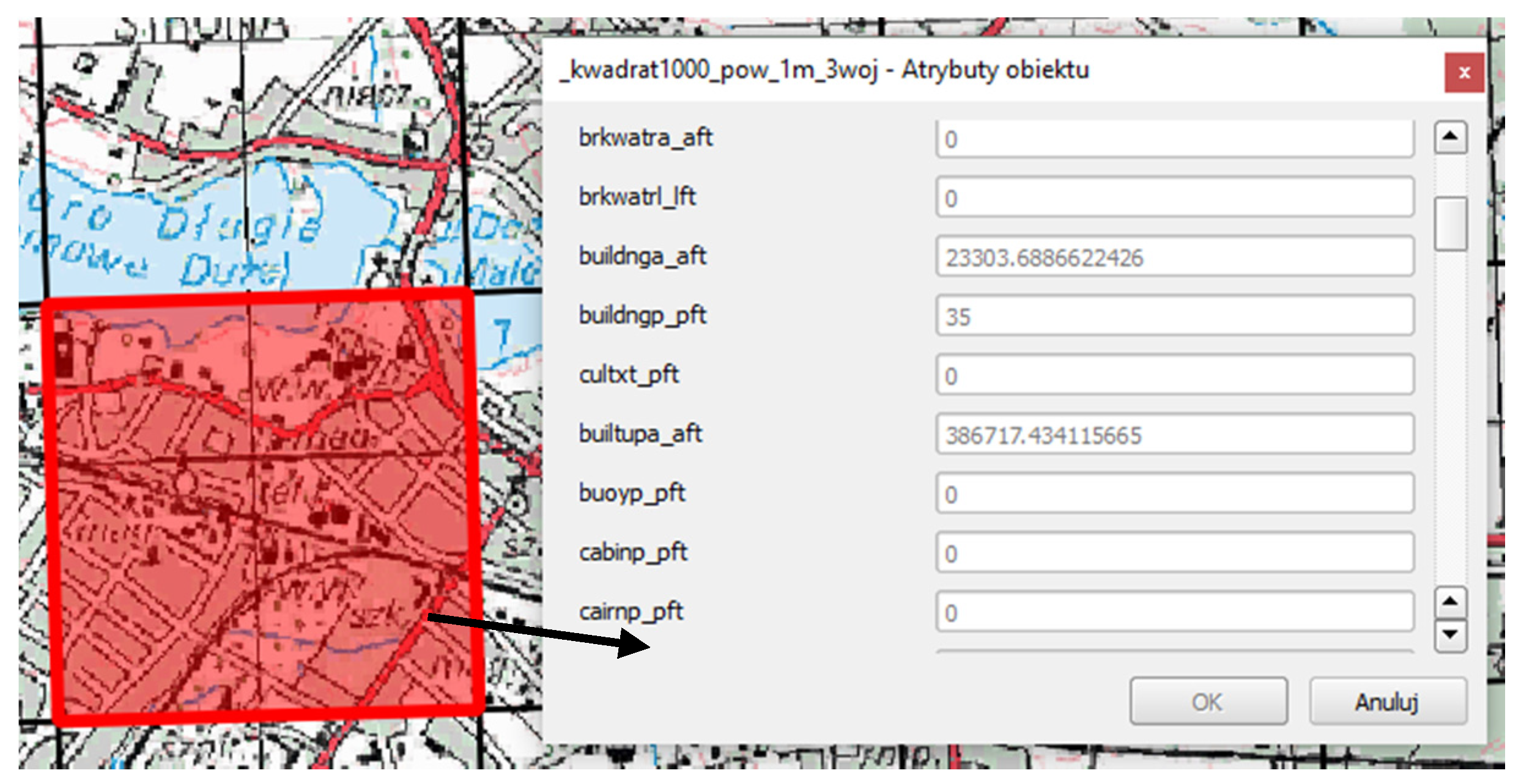
Additionally, apart from the data about land cover elements, the average value of the elevation and slope was determined for each cell on the basis of SRTM L1 numerical terrain model [38] and numerical terrain slope model created by authors. These values were defined based on all measurement points contained in the given cell. An example of the set of parameters for each cell is presented in Figure 1.

Passability maps were generated with the use of the automated terrain classification method, based on the determination of the index of passability. As opposed to the traditional methods that determined only three classes of passability [18], in the present study, the index of passability is generated in continuous range increments from 0.0 (impassable terrain) to 1.0 (perfect manoeuvrability terrain) [32]. The determination of the index of passability was based on the vegetation roughness factor (VRF, denoted I_VRF), which is a numerical evaluation reflecting the degree of the speed limit related to the movement of vehicles through the different types of land cover [19], defined with the use of the so-called resistance coefficient. As a result of that, this method is referred to as the “VRF method”. During the tests, each class of objects from VMap Level 2 was assigned a resistance coefficient. Terrain objects were divided into those that hinder (I_VRF < 0), facilitate (I_VRF > 0), or do not affect passability (I_VRF = 0). As a result of this operation, 112 feature classes that do not affect passability (mainly singular objects), 99 hindering, and 10 facilitating traversing the area were isolated. Open terrain (not covered with surface objects) was also classified as a facilitator. This area was assigned a resistance coefficient of +0.5. Sample values of the resistance coefficient are presented in

Table 1. Sample vegetation roughness factor (VRF) values.

Facilitating		Hindering		Neutral
Object	IVRF	Object	IVRF	Object	IVRF
Roads	0.7	River	−1.0	Monument	0
Footpath	0.4	Swamp	−0.8	Tree	0
Firebrake	0.3	Forest (area)	−0.8	Chimney	0
Tunell	0.2	Orchard	−0.5	Forest (point)	0
Open areas (without area objects)	0.5	Slope	−0.4	All cartographic elements (e.g., labels)	0

, and the detailed description of the manner of determining the index of passability based on VRF is described in Pokonieczny [20].

Apart from passability maps with marked total index of passability (taking into account all feature classes covered by VMap Level 2), the method described above was used to develop maps that reflect terrain passability according to basic types of land cover and relief. They were generated by calculating IOP only for classes of objects included in the given thematic category. Maps were generated for the following categories: buildings, formation, hydrography, and vegetation, with the use of feature classes listed in

Table 2. Feature classes (according to DIGEST) used for generating passability maps according to specific feature classes.

Built-up	Relief	Hydrography	Vegetation
airporta_aft, athlflda_aft, buildnga_aft, buildngp_pft, builtupa_aft, campsita_aft, cemetrya_aft, conveyl_lft, cooltowp_pft, damc_pft, daml_lft, depota_aft, disposa_aft, drydocka_aft, farmp_pft, fencel_lft, firernga_aft, fortifna_aft, grainela_aft, locka_aft, minea_aft, piera_aft, pita_aft, pitp_pft, plazaa_aft, powerpla_aft, procplta_aft, pumpsta_aft, quarrya_aft, skijumpp_pft, slipwaya_aft, stadiuma_aft, zooa_aft	bluffl_lft, cairnp_pft, cavep_pft, cutl_lft, embanka_aft, embankl_lft, grassa_aft, gullyl_lft, minpilea_aft, minpilep_pft, sandunea_aft, steepgrl_lft, slope	anchora_aft, anchorp_pft, canala_aft, canall_lft, ditcha_aft, ditchl_lft, fishfrma_aft, lakea_aft, reservra_aft, rivera_aft, riverl_lft, setbasa_aft, swampa_aft, swampp_pft, watera_aft, wtrfalll_lft	cropa_aft, bambooa_aft, boga_aft, foresta_aft, forestl_lft, hedgel_lft, hopsa_aft, orchara_aft, parka_aft, scruba_aft

. This approach is compliant with standardisation documents [19] that recommend generating passability maps according to various types of objects (i.e., separate passability maps for vegetation, hydrography, relief, etc.).

2.2. Test Area

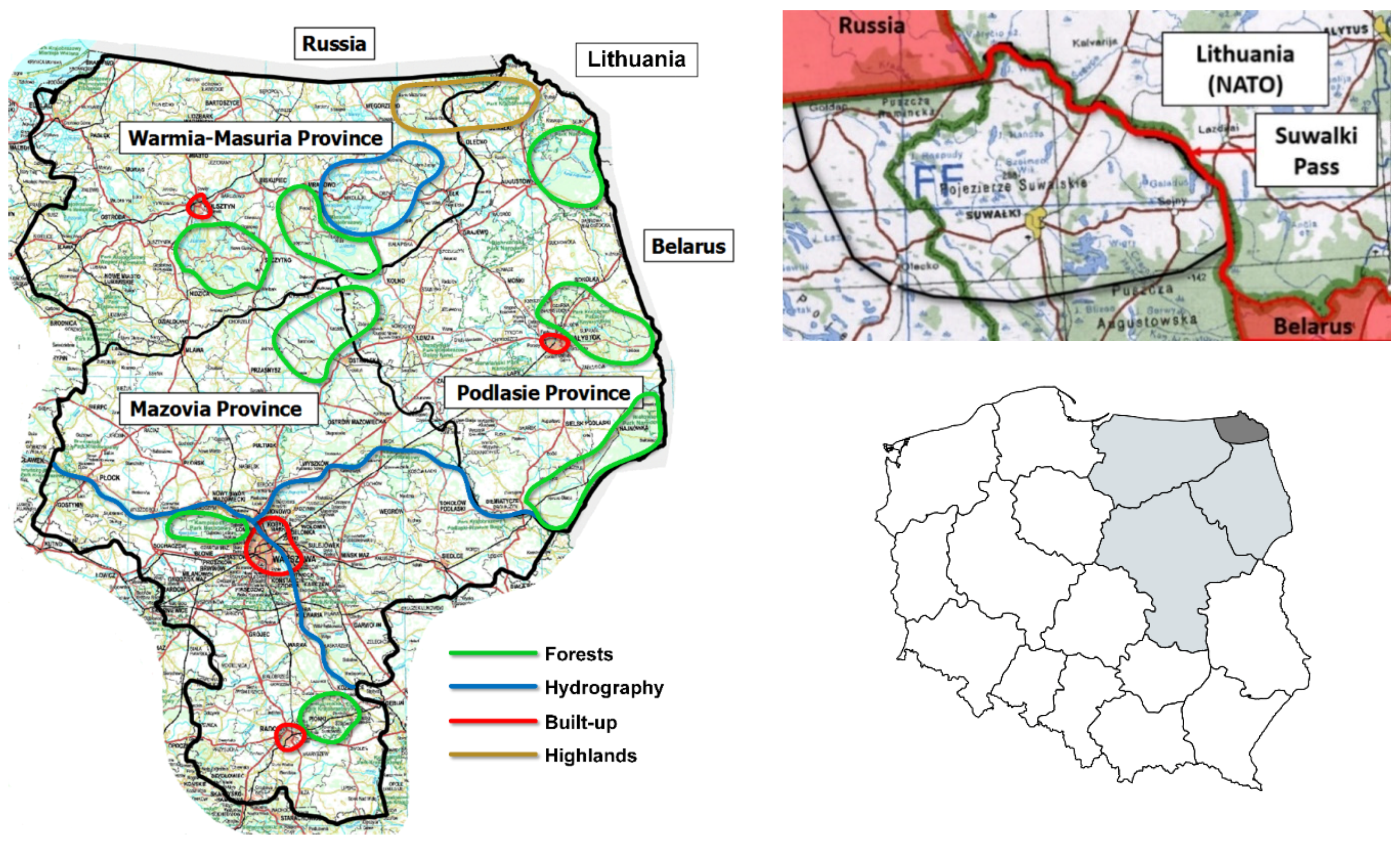
Tests related to the selection of the shape of cells were conducted on the area of three provinces in North-Eastern Poland (Masovia, Warmia-Masuria, and Podlasie Province) (Figure 2, left side). This region is the area of interest of both Polish Armed Forces and of NATO (North Atlantic Treaty Organization), as it is directly adjacent to the territory of the Russian Federation. This is an area of approximately 81,000 km², characterised by diversified land cover elements, which influence passability. It encompasses the largest water reservoirs in Poland (the Great Masurian Lakes), two large water courses (the Vistula and Bug Rivers), as well as large forest areas (covering 27% of the analysed area). The northern section of the test region contains both large slopes (up to 10°) and vast plains (e.g., the Łowicz-Błonie Plain). The test area also includes the Warsaw Agglomeration and two provincial capitals (Białystok and Olsztyn). The density of the road network varies and depends on the degree of land development.

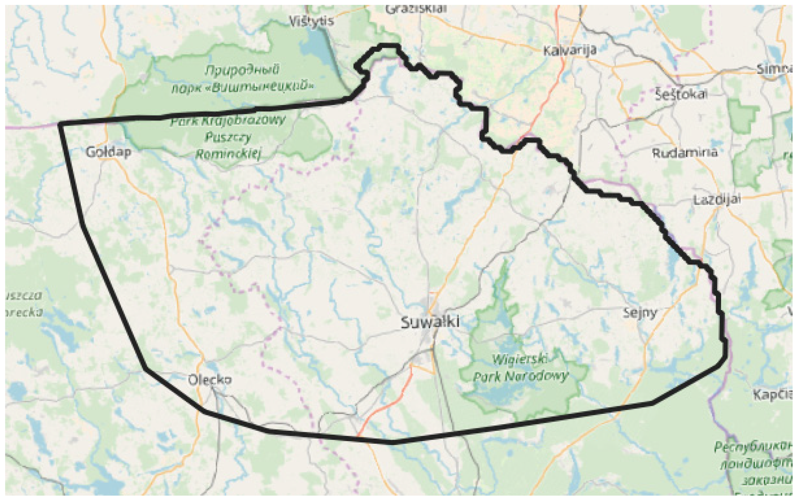
For the purposes of research on the size of the cells, the test area was limited to a fragment of a surface area of 5000 km², located in the north-eastern section of the three mentioned provinces’ areas. It contains the so-called “Suwałki Pass” (Figure 2, right side, on the top). The Suwalki Pass (also called the Suwalki Gap) is considered to be a likely location of the initial direction of attack in the event of a war initiated by Russia [39]. The importance of the Suwalki Gap results from its geostrategic location. It is located on the 100-km long Polish–Lithuanian border, surrounded by Belarus and the Kaliningrad Region, and is connected with the threat posed by the Russian Federation to the security of the Baltic states and, in general, towards NATO and the European Union. The challenge results from the fact that this borderline is of importance for the Alliance because of an obligation towards Estonia, Latvia, and Lithuania under Article V of the Washington Treaty. It is a relatively narrow isthmus that (if blocked) would make it possible to cut the Baltic states off from the rest of NATO countries.

The terrain formation of the analysed area is quite diversified (Figure 3). It is characterised by post-glacial landscape, with a large number of post-glacial lakes, upland hills, moraines, and outwash plains. A dense network of low hills, whose height ranges from several to 50 m, and whose diameter ranges from 100 to 500 m, is arranged in latitudinal hill ranges. The inclinations of slopes usually range from 2 to 15°. Throughout the area, hills are separated by numerous depressions without outlet (basins), whose diameter ranges from over ten meters to several kilometres. An important feature of the terrain formation are post-glacial tunnel valleys—elongated depressions with steep, usually wooded slopes that are usually stretched in the north-west to south-east direction. These valleys usually contain long, narrow lakes or rivers and peat bogs. The height of the tunnel valley slopes reaches 30–60 m at some points, and the slope inclinations range from 8–30°. In hypsometric terms, the altitudes above sea level in the operating region range from 0 m on the borders of the depression south of Elbląg to 309 m (Szeska Góra). However, a majority of the area lies on elevations ranging from 100 to 200 m.

Approximately 35% of the analysed area is covered by forests. The largest forest complexes are the Skaliskie Woods, Puszcza Borecka, Puszcza Romnicka, and Puszcza Augustowska. The forests are located unevenly. The largest woods occur in the Olsztyn, Mrągowo, Iława Lake Districts, on the Masurian Plain, and on the Augustów Plain. These are mainly coniferous forests, strongly dominated by pine, growing mainly on sandy soils.

The analysed area contains multiple rivers with small catchments and uneven inclinations (e.g., Czarna Hańcza). Rivers flow down in different directions from the moraine hills in the lake district zone. The analysed area is, first of all, the “Land of a Thousand Lakes”, as it contains the largest number of lakes in Poland. Some of them are tunnel valley lakes that are connected to Mamry and Śniardwy with a system of channels that create a branching shipping route. Nearly all of the lakes are of glacial origin. The lakes in the Augustów Plain are connected to the Czarna Hańcza and Biebrza Rivers by the Augustów Channel. The deepest lake both in the region and in Poland is the Hańcza Lake.

The population density in the analysed area is low (approx. 50 people/km²). Three large towns are located in the area: Gołdap, Olecko, and Suwałki. Suwałki, with a population of 68,000, is the capital of the mesoregion. It is the largest city of the Lake District, situated on the Czarna Hańcza River. The city is located at the international road that leads to Lithuania and to other Baltic States. It is an important local railroad hub, where the railways from Sokółka, Lithuania, and Olecko meet. The town has developed wood, construction, food processing, and clothing industries.

2.3. Analysis of the Shape of Cells

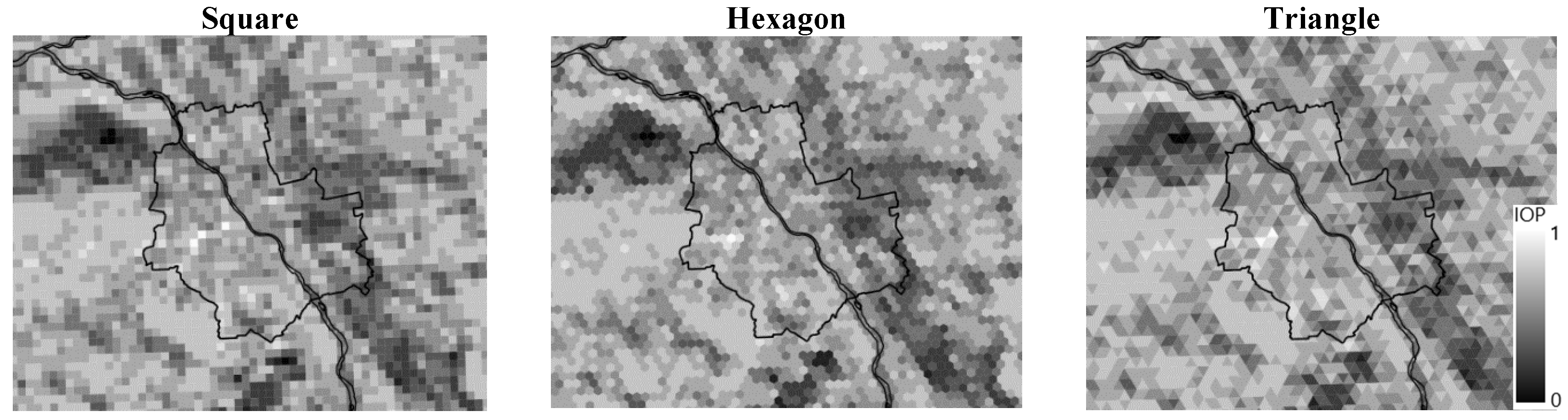
Indices of passability calculated on the basis of parameters derived from land cover elements from VMap Level 2, and with use of the VRF method, were determined for square, triangular, and hexagonal cells, of the same surface area of 1 km². The test area was divided into 81,032 square cells, 81,220 cells of a shape of an equilateral triangle, and 81,023 cells of a shape of a regular hexagon.

Indices of passability constituted the basis for the development of three passability maps for the three different shapes of cells (square, hexagon, and triangle). The obtained results were analysed by determining the values of indices of passability in independent control points, located in the same places on three generated maps. The VRM (Vegetation Roughness Factor) method was also used. Control points were distributed on each map in three variants (Figure 4):

• on a point grid with an interval of 1000 m (80,121 points);
• on a point grid with an interval of 5000 m (3203 points);
• at 1000 points whose location was determined randomly.

For each control point, the IOP of the cell where the given point was located was read. As a result of the fact that the index of passability is determined on a continuous scale, the authors also checked the percentage of control points—for three adopted variants of cell shapes—for which the difference in the value of the index of passability between the analysed cell shapes did not exceed ±0.1.

In order to analyse the differences between three developed terrain passability maps, a matrix of correlations between the indices of passability assigned to control points established in three distribution variants (1000 and 5000 m grid, 1000 randomly distributed points) was determined. Additionally, basic statistics (mean and standard deviation) were calculated for indices of passability obtained in control points.

2.4. Analysis of the Size of the Cells

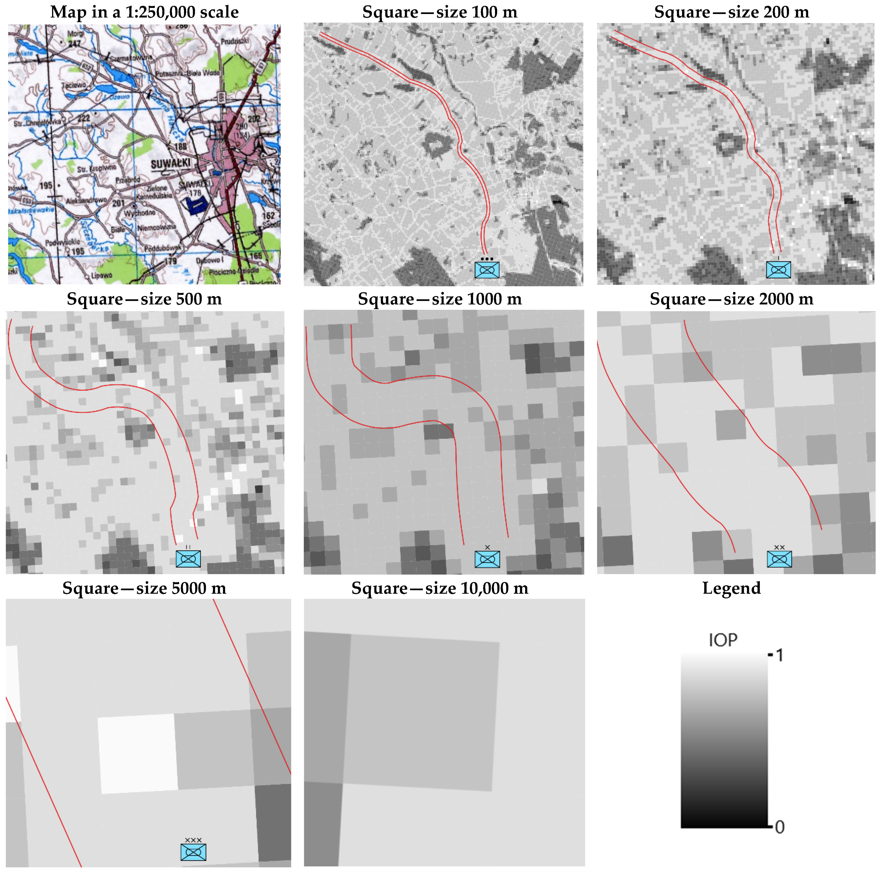
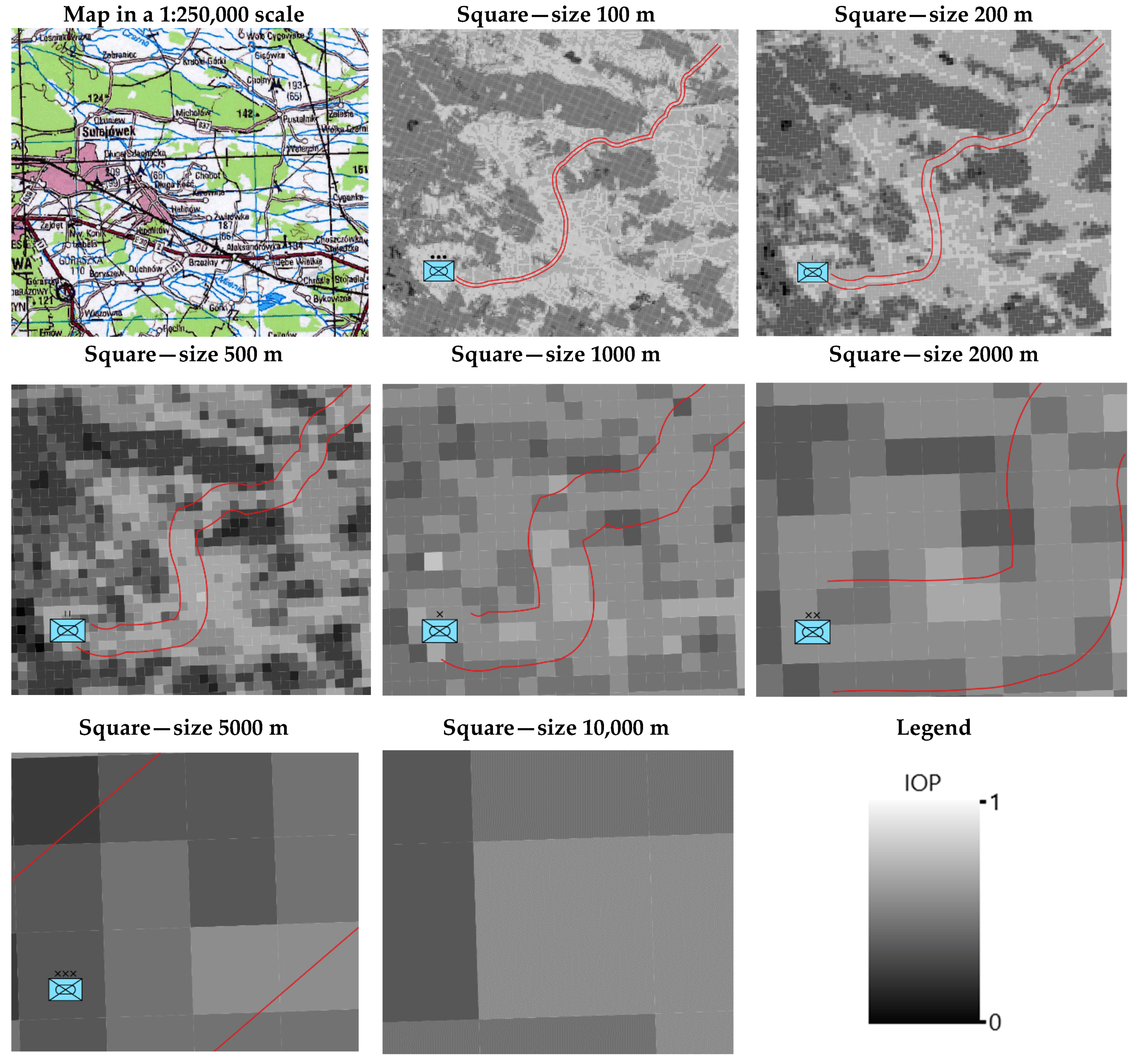
During the research, indices of passability were determined for cells of the same shape, but different sizes. Tests were conducted for square shaped cells. In the analysed area (the Suwałki Pass, Figure 2, right side, on the top), cells of the sizes of 100 m, 200 m, 500 m, 1000 m, 2000 m, 5000 m, and 10,000 m were generated. The indices of passability were determined for these cells, based on land cover parameters generated with use of data from VMap Level 2 and the VRF method. The calculated indices were then used to create passability maps for each of the analysed cell sizes (i.e., seven maps were obtained).

Similar to in the tests of cell shape, control points were distributed in the test area in three configurations (Figure 5), the same as for the cell shape analysis, that is, on a grid of 1000 m and 5000 m mesh, and 1000 randomly distributed points. Indices of passability were read for the control points on each of the generated maps. As a result, each control point (in three configurations) was assigned the values of seven indices of passability (separately for each cell size).

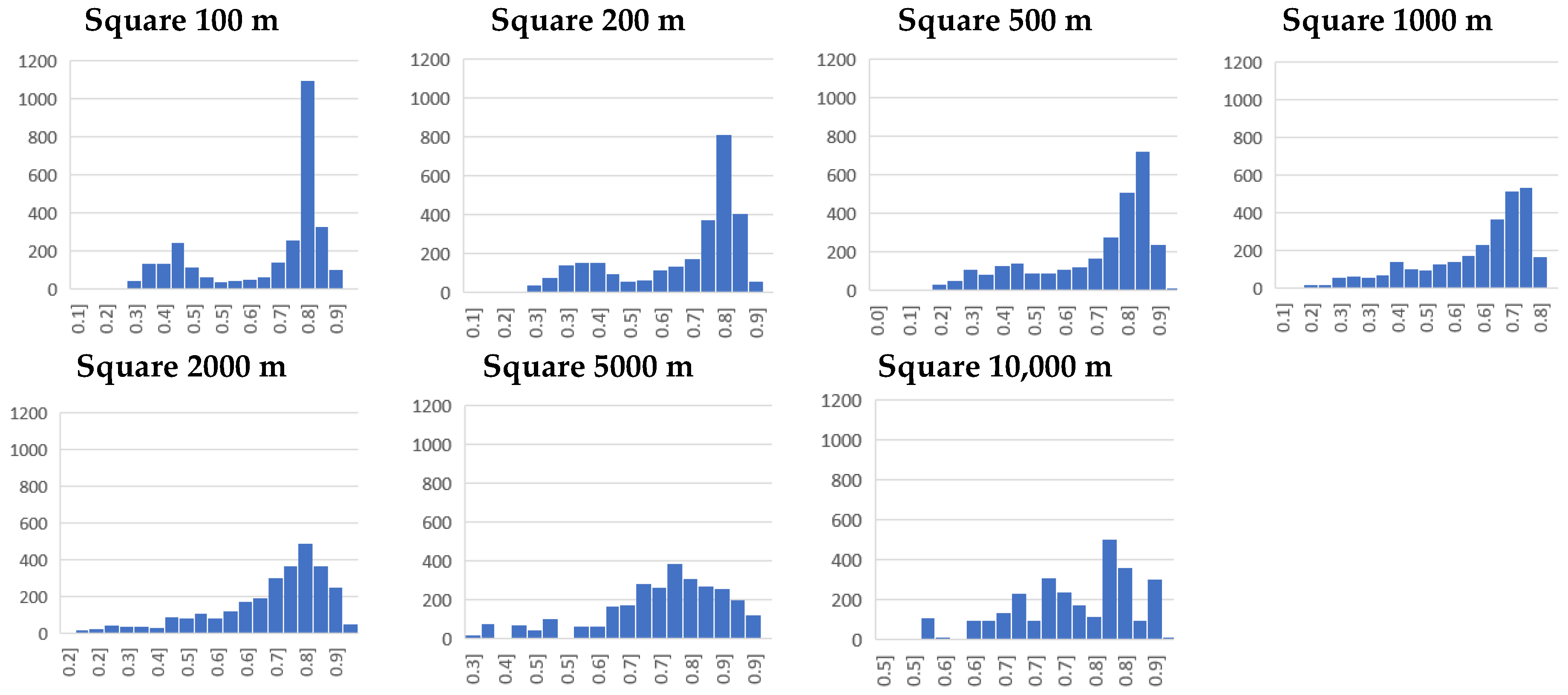
In order to analyse the differences between the generated passability maps, matrices of correlation between the indices of passability obtained for control points in the three variants were developed. To determine the distribution of the obtained indices of passability, histograms were generated and basic statistics (average, standard deviation) were calculated to describe the distribution of indices of passability for different sizes of cells.

As a result of the possibility of using passability maps of various levels of detail for different military purposes it was assumed that the maps generated for various cell sizes should meet the needs of the armed forces on the levels of a company, battalion, brigade, division, and corps. As a result of that, the sizes of the analysed cells referred to the width of the avenues of approach depending of the size of the given military unit. The width of the avenues of approach and the map scales used for the passability maps purposes are defined in U.S. Army [40]. To present the width of the avenue of approach on the map, the size of the cell should be smaller than these widths of avenues in map scale. Therefore, the authors have proposed cell sizes related to the width of the avenue of approach, and they are based on the rule that the cell size cannot be bigger (in map scale) than half of the avenue width. The proposed values are 1/2 or 1/3 of the avenue width. The correlations between the size of the troops, width of the avenue of approach, and the adopted cell sizes proposed by the authors are presented in

Table 3. Correlation between troop size, width of the avenue of approach, and the adopted cell size.

Troop Size	Troop Symbol (MIL-STD-2525C)	Size of Cell	Scale of Used Topographic Map	Width of Avenue of Approach
Platoon		100 m	1:25,000	200 m
Company		200 m	1:50,000	500 m
Battalion		500 m		1500 m
Brigade		1000 m	1:100,000	3000 m
Division		2000 m		6000 m
Corps		5000 m	1:250,000	15,000 m

.

The tests also involved a comparison of the time of preparation of passability maps generated with the use of automatic terrain classification with the time of preparation of maps created manually in military units. The studies involved generating maps with use of the VRF method and VMap Level 2 data for cells of various sizes covering the same area, that is, the Suwałki Pass.

2.5. Comparison of Maps Generated Automatically and Traditionally

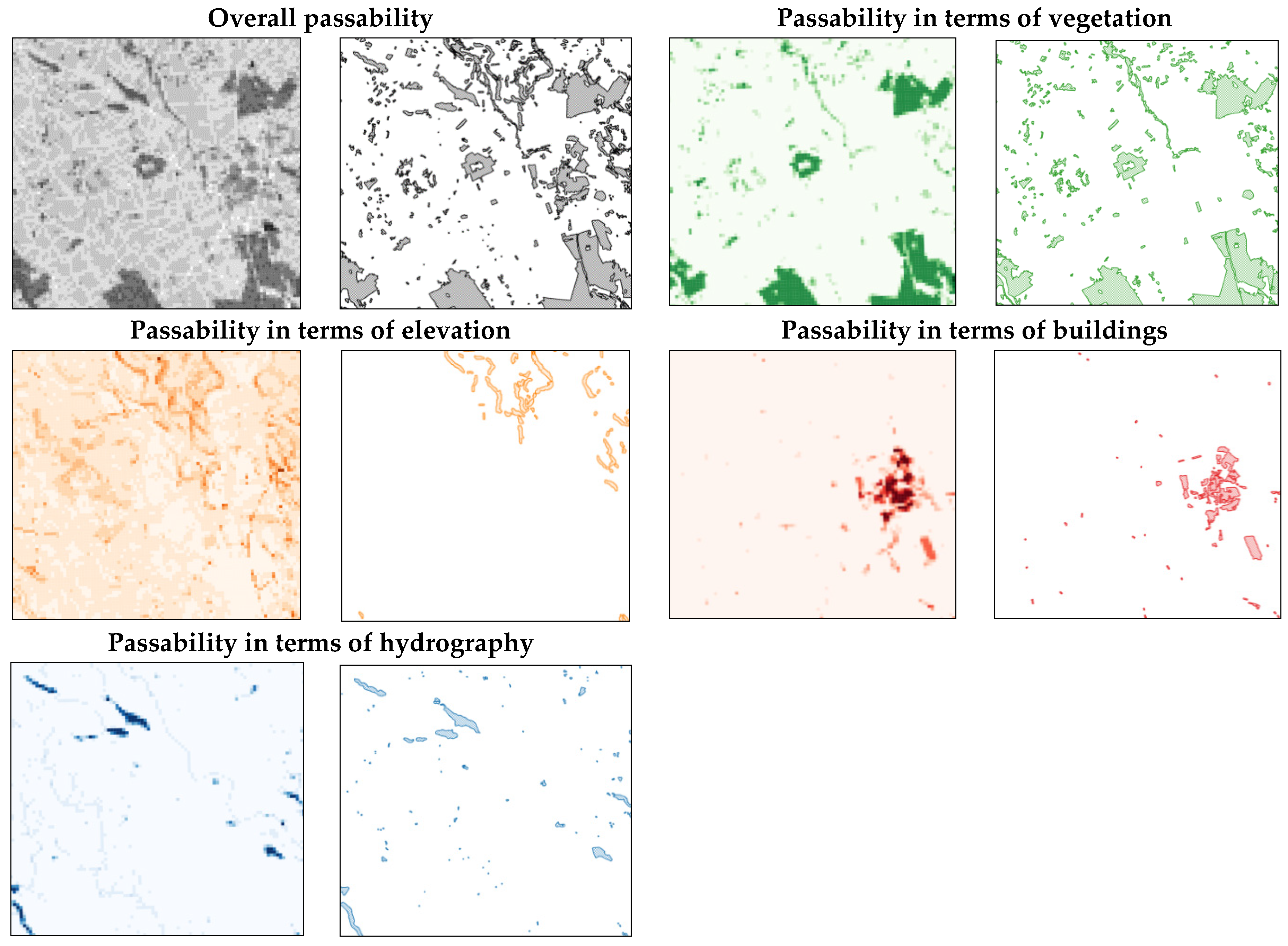
The experiment consisted of comparing the generated passability maps of various cell sizes with a map compiled manually by an experienced operator, that is, the officer of reconnaissance section who knows the area of interest and who designed a lot of passability maps with the use of analogue maps. The experiment was based on the traditional method of creating passability maps based on military standardisation documents [18]; a universal passability map was created for various troop levels. Standard, military cartographic materials were used (topographic maps in various scales and ortophotomaps). Pursuant to the provisions of standardisation documents [41], the process of generating passability maps involved distinguishing GO and NO GO areas (

Table 4. Passability classes according to standardisation documents.

	GO	SLOW GO	NO GO
Forests	Trees with a diameter of less than 5 cm or the distance between trees with any diameter of greater than 5 m	Trees with a diameter from 5 to 15 cm, and the distance between them of less than 5 m	Trees with a diameter grater then 15 cm and the distance between them of less than 5 m
Roads	two or more of paved roads per km2	one paved road or two unpaved on km2	one paved road on km2
Hydrography	width less than 1.5 m and a depth of less than 0.6 m	the height of the banks of to 1.2 m, the speed stream of 1.5 m/s, a depth of 1.2 m	banks with a height of over 1.2 m, speed stream greater than 1.5 m/s, depth greater than 1.2 m
Built-up area	not included	not included	areas of size more than 1 km2
Topography	slopes less than 30%	slopes between 30 and 50%	slopes more than 50%
Slopes	area with a height difference from 0 to 100 m per km	area with a height difference from 100 to 200 m per km	area with a height difference from 200 to 400 m per km

) according to the basic categories of land cover and relief, vegetation, buildings, relief, and hydrography. All maps were created manually by marking NO GO and SLOW GO areas.

Traditionally and automatically generated maps were compared in the same way as the comparison of passability maps generated for various cell sizes—by overlaying control points in three configurations on the maps. At the same time, on manually generated maps, the index of passability for NO GO areas was set to 0, and for SLOW GO areas to 0.5, while areas not marked on the maps were a priori considered as passable, and assigned a 1.0 index of passability. Correlation coefficients and basic statistics (average, standard deviation) were calculated for the obtained data sets.

2.6. Checking the Correctness of the Proposed Solutions

In order to verify the correctness and universality of the presented method of automated passability maps generation, the final experiment was conducted. It consisted of generating maps for a cell of squares of the same dimensions (from 100 m to 10,000 m), as for the Suwałki Pass area. The tests were conducted in a different region, with the use of a different spatial data base. Maps were generated with the use of an identical method, such as those created for the Suwałki Pass area (the VRF method).

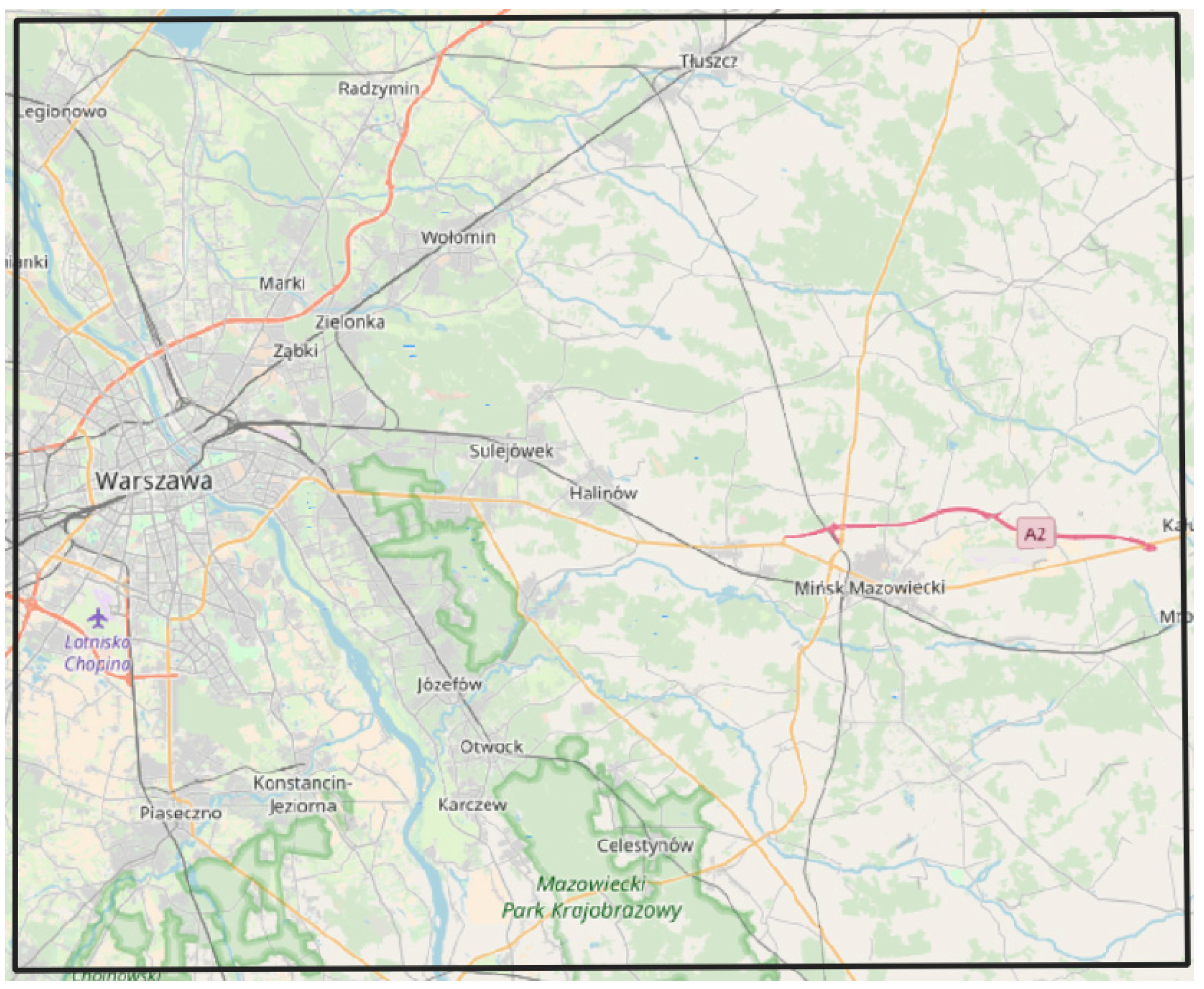
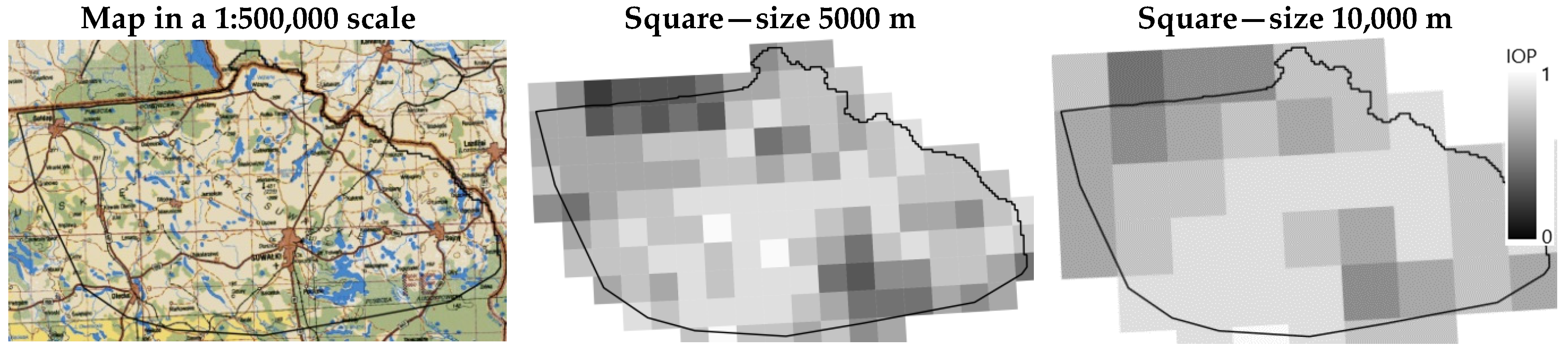
The new test site has a similar surface area as the analysed Suwałki Pass region (approx. 3000 km²). It covers a part of the Central Vistula Valley, the Warsaw Basin, and the Wołomin Plain. The intention of the authors was for the area to differ from the analysed Suwałki Pass area as much as possible. As opposed to the latter, this region is densely populated (as it includes the Warsaw Agglomeration). It does not contain any major denivelations or large lakes. The main hydrographic element is the Vistula River. The selected region is highly developed. Additionally, it has a dense network of roads (including national roads and expressways) and railroads. Dense, consistent forest areas exist in its central and eastern parts. The location of the new area is presented in Figure 6.

As opposed to the maps generated for the Suwałki Pass area, which were created with the use of VMap Level 2, the tests conducted for the Warsaw Agglomeration were based on the generally available spatial database OpenStreetMap, which is a project developed by the Internet community. The main aim of this project is to create a free-of-charge, freely accessible map of the whole globe. Data for this database are collected by registered users and based on recorded GPS (Global Positioning System) tracking, satellite photos, maps to which the copyrights have expired, and own knowledge about the edited area. Apart from general geographic information, the database contains descriptive information in form of POI—points of interest.

Similar to in the previously discussed experiments, matrices of correlation between the indices of passability obtained for control points in the three variants were developed (on a grid of 1000 m and 5000 m mesh, and 1000 randomly distributed points). To determine the distribution of the obtained indices of passability, basic statistics were calculated to describe the distribution of indices of passability for different sizes of cell (average, standard deviation).

To demonstrate the degree of similarity between individual maps, the Pearson correlation coefficient (PCC) was calculated [42]. The Pearson correlation was selected because the covariances were calculated based on empirical data, taken from the maps.

3. Results

3.1. Results of the Cell Shape Analysis

As a result of the tests, indices of passability were determined for square, triangular, and hexagonal cells. They constituted the basis for generating passability maps. Fragments of the created maps are presented in Figure 7. Correlation matrices determining the correlations between indices of passability calculated for cells in three variants, for all three control point configurations, are presented in

Table 5. Correlation matrix and basic statistic parameters.

Cell Shape	Average	Standard Deviation	Square	Hexagon	Triangle
1000 m grid, 80,121 points
Square	0.611	0.141	1.000	0.773	0.752
Hexagon	0.611	0.141	-	1.000	0.831
Triangle	0.618	0.142	-	-	1.000
5000 m grid, 3203 points
Square	0.611	0.141	1.000	0.780	0.744
Hexagon	0.610	0.143	-	1.000	0.833
Triangle	0.617	0.142	-	-	1.000
1000 randomly distributed points
Square	0.610	0.143	1.000	0.888	0.841
Hexagon	0.612	0.142	-	1.000	0.829
Triangle	0.622	0.142	-	-	1.000

.

To analyse the correlation between passability maps, the Pearson correlation coefficient has been calculated. It was used, instead of the fact that the distribution of the values is not normal. According to the literature [43], tests based on normality can be used, provided we have a sufficiently large sample. This possibility is based on an extremely important claim that tests based on normal distribution are of huge importance. Fisher claims that as the sample size increases, the distribution of the test statistics based on the average approaches the normal distribution, regardless of the distribution of the variable that we measure.

The sample size used in the research is large: from 1000 to 80,000 control points. Therefore, also according to the law of large numbers, the sample correlation coefficient is a consistent estimator of the population correlation coefficient.

The percentage of control points for which the difference between indices of passability is lower than 0.1, for all three variants of control point distribution, is presented in

Table 6. Percentage of control points for which the difference between indices of passability does not exceed 0.1.

	Square	Hexagon	Triangle
1 000 m grid, 80,121 points
Square	100%	77%	76%
Hexagon		100%	82%
Triangle			100%
5 000 m grid, 3203 points
Square	100%	78%	75%
Hexagon		100%	82%
Triangle			100%
1000 randomly distributed points
Square	100%	84%	87%
Hexagon		100%	83%
Triangle			100%

.

3.2. Results of the Cell Size Analysis

The indices of passability determined for various cell sizes were a basis for generating passability maps on various levels of detail. Fragments of maps created for various sizes of square shaped cells are presented in Figure 8. Exemplary avenues of approach based on parameters defined in Table 3 have been drawn on the maps.

The Pearson correlation matrices that demonstrate the degree of similarity between individual maps are presented in

Table 7. Correlation matrix and basic statistic parameters for the 1000 m mesh control points grid.

Side Length	Average	Standard Deviation	100 m	200 m	500 m	1000 m	2000 m	5000 m	10,000 m
100 m	0.664	0.190		0.924	0.897	0.803	0.685	0.512	0.367
200 m	0.662	0.190	0.924		0.944	0.848	0.719	0.547	0.393
500 m	0.684	0.187	0.897	0.944		0.904	0.789	0.598	0.431
1000 m	0.604	0.151	0.803	0.848	0.904		0.868	0.663	0.482
2000 m	0.666	0.155	0.685	0.719	0.789	0.868		0.743	0.559
5000 m	0.710	0.136	0.512	0.547	0.598	0.663	0.743		0.767
10,000 m	0.750	0.096	0.367	0.393	0.431	0.482	0.559	0.767
		Average	0.708	0.712	0.755	0.760	0.738	0.656	0.519

,

Table 8. Correlation matrix and basic statistic parameters for the 5000 m mesh control points grid.

Side Length	Average	Standard Deviation	100 m	200 m	500 m	1000 m	2000 m	5000 m	10,000 m
100 m	0.669	0.184		0.933	0.896	0.832	0.698	0.634	0.450
200 m	0.659	0.188	0.933		0.928	0.833	0.705	0.654	0.485
500 m	0.681	0.190	0.896	0.928		0.901	0.805	0.730	0.537
1000 m	0.592	0.159	0.832	0.833	0.901		0.845	0.755	0.516
2000 m	0.660	0.156	0.698	0.705	0.805	0.845		0.849	0.663
5000 m	0.711	0.136	0.634	0.654	0.730	0.755	0.849		0.765
10,000 m	0.751	0.093	0.450	0.485	0.537	0.516	0.663	0.765
		Average	0.708	0.712	0.755	0.760	0.738	0.656	0.519

and

Table 9. Correlation matrix and basic statistic parameters for 1000 randomly selected control points.

Side Length	Average	Standard Deviation	100 m	200 m	500 m	1000 m	2000 m	5000 m	10,000 m
100 m	0.654	0.197		0.932	0.865	0.790	0.702	0.556	0.399
200 m	0.652	0.197	0.932		0.870	0.800	0.713	0.554	0.404
500 m	0.672	0.193	0.865	0.870		0.904	0.809	0.619	0.461
1000 m	0.593	0.157	0.790	0.800	0.904		0.876	0.682	0.511
2000 m	0.651	0.164	0.702	0.713	0.809	0.876		0.753	0.573
5000 m	0.700	0.140	0.556	0.554	0.619	0.682	0.753		0.769
10,000 m	0.745	0.098	0.399	0.404	0.461	0.511	0.573	0.769
		Average	0.708	0.712	0.755	0.760	0.738	0.656	0.519

. These matrices, together with the basic statistic parameters were generated separately for three control point configurations.

The distribution of the generated indices of passability for each tested cell size is presented in the histograms in Figure 9, Figure 10 and Figure 11. They were generated separately for three control point configurations.

3.3. Results of the Comparison between Generated Passability Maps and Maps Created Manually

The analysis of cartographic materials used by the Polish Armed Forces resulted in the creation of a military passability map generated by marking NO GO and SLOW GO areas manually on the analysed area. Figure 12 shows fragments of this map divided into thematic categories and their comparison with passability maps generated for a square cell of the side length of 200 m.

The correlation matrices that demonstrate the degree of similarity between passability maps generated with use of the VRF method are presented in

Table 10. Correlation matrices and basic statistic parameters for the 5000 m mesh control points grid.

			Side Length of Grid Square
	Average	Standard deviation	100 m	200 m	500 m	1000 m	2000 m	5000 m	10,000 m
Correlation matrix (passability)
Manually created map	0.705	0.451	0.835	0.742	0.783	0.723	0.608	0.540	0.380
Correlation matrix (vegetation)
Manually created map	0.761	0.429	0.829	0.782	0.787	0.723	0.654	0.605	0.449
Correlation matrix (elevation)
Manually created map	0.987	0.079	0.363	0.201	0.312	0.230	0.127	0.196	0.203
Correlation matrix (buildings)
Manually created map	1.000	0.000	Determination was impossible, as the land was passable for all control points.
Correlation matrix (hydrography)
Manually created map	0.949	0.222	0.742	0.544	0.645	0.526	0.315	0.095	-0.049

,

Table 11. Correlation matrices and basic statistic parameters for the 1000 m mesh control points grid.

			Side Length of Grid Square
	Average	Standard deviation	100 m	200 m	500 m	1000 m	2000 m	5000 m	10,000 m
Correlation matrix (passability)
Manually created map	0.696	0.451	0.872	0.768	0.772	0.688	0.572	0.393	0.287
Correlation matrix (vegetation)
Manually created map	0.751	0.432	0.885	0.798	0.790	0.712	0.587	0.440	0.325
Correlation matrix (elevation)
Manually created map	0.983	0.096	0.477	0.367	0.433	0.323	0.249	0.168	0.142
Correlation matrix (buildings)
Manually created map	0.993	0.084	0.799	0.542	0.552	0.399	0.284	0.152	0.109
Correlation matrix (hydrography)
Manually created map	0.946	0.226	0.871	0.705	0.711	0.568	0.411	0.149	0.101

and

Table 12. Correlation matrices and basic statistic parameters for 1000 randomly selected control points.

			Side Length of Grid Square
	Average	Standard deviation	100 m	200 m	500 m	1000 m	2000 m	5000 m	10,000 m
Correlation matrix (passability)
Manually created map	0.714	0.445	0.882	0.837	0.760	0.685	0.607	0.445	0.323
Correlation matrix (vegetation)
Manually created map	0.761	0.426	0.894	0.848	0.779	0.709	0.624	0.486	0.384
Correlation matrix (elevation)
Manually created map	0.990	0.072	0.375	0.329	0.309	0.238	0.214	0.143	0.125
Correlation matrix (buildings)
Manually created map	0.996	0.063	0.740	0.701	0.493	0.301	0.231	0.085	0.014
Correlation matrix (hydrography)
Manually created map	0.949	0.220	0.900	0.813	0.657	0.554	0.449	0.142	0.120

. These matrices, together with the basic statistic parameters, were generated separately for three control point configurations. The tables also contain correlation matrices and basic statistical parameters calculated for maps considering specific categories of spatial objects (vegetation, relief, buildings, and hydrography).

The total map generation time consists of the following: preparation of the data model (square cells) and direct calculation of the index of passability. The results of these operations for the Suwałki Pass area are presented in

Table 13. Map generating time.

Square Side Length	Number of Squares in Tested Area	Time of Data Model Preparation	IOP Generating Time	Total Map Generating Time
100 m	295,772	90 h 22 min	2 h 28 min	92 h 50 min
200 m	74,317	22 h 42 min	0 h 37 min	23 h 20 min
500 m	12,060	3 h 41 min	0 h 6 min	3 h 47 min
1000 m	3085	0 h 57 min	0 h 2 min	1 h 0 min
2000 m	808	0 h 15 min	0 h 1 min	0 h 16 min
5000 m	147	0 h 3 min	>0 h 1 min	0 h 4 min
10,000 m	44	0 h 1 min	>0 h 1 min	0 h 2 min
Manual creation of passability map of the analysed area, pursuant to [19]				approx. 20 h

. Calculations were performed on a computer with Intel Xeon e3-1230 v5 3, 4 GHz (4 cores) processor, memory: 8 GB DDR IV. For this hardware configuration, the time of preparation of the data model for one square (regardless of its size) is 1.1 s. Calculation of IOP for one square takes approximately 0.03 s.

3.4. Results of Checking the Proposed Solution for a Different Area and Dataset

Fragments of passability maps for the Warsaw Agglomeration region, generated with use of the VRF method and the OpenStreetMap data are presented in Figure 13. The maps also contain sample avenues of approach, entered in compliance with the parameters listed in Table 3.

The Pearson correlation matrices that demonstrate the degree of similarity between individual maps are presented in

Table 14. Correlation matrix and basic statistic parameters for the 1000 m mesh control points grid.

Side Length	Average	Standard Deviation	100 m	200 m	500 m	1000 m	2000 m	5000 m	10,000 m
100 m	0.581	0.126		0.922	0.700	0.528	0.452	0.321	0.274
200 m	0.541	0.147	0.922		0.825	0.620	0.518	0.343	0.276
500 m	0.454	0.140	0.700	0.825		0.840	0.649	0.417	0.273
1000 m	0.527	0.145	0.528	0.620	0.840		0.789	0.503	0.302
2000 m	0.517	0.141	0.452	0.518	0.649	0.789		0.607	0.361
5000 m	0.467	0.146	0.321	0.343	0.417	0.503	0.607		0.706
10,000 m	0.403	0.209	0.274	0.276	0.273	0.302	0.361	0.706
		Average	0.533	0.584	0.617	0.597	0.563	0.483	0.365

,

Table 15. Correlation matrix and basic statistic parameters for the 5000 m mesh control points grid.

Side Length	Average	Standard Deviation	100 m	200 m	500 m	1000 m	2000 m	5000 m	10,000 m
100 m	0.580	0.133		0.907	0.641	0.481	0.463	0.199	0.200
200 m	0.535	0.153	0.907		0.796	0.588	0.582	0.258	0.263
500 m	0.449	0.142	0.641	0.796		0.869	0.747	0.302	0.268
1000 m	0.527	0.147	0.481	0.588	0.869		0.816	0.361	0.235
2000 m	0.515	0.153	0.463	0.582	0.747	0.816		0.462	0.293
5000 m	0.470	0.144	0.199	0.258	0.302	0.361	0.462		0.710
10,000 m	0.409	0.208	0.200	0.263	0.268	0.235	0.293	0.710
		Average	0.482	0.566	0.604	0.558	0.560	0.382	0.328

and

Table 16. Correlation matrix and basic statistic parameters for 1000 randomly selected control points.

Side Length	Average	Standard Deviation	100 m	200 m	500 m	1000 m	2000 m	5000 m	10,000 m
100 m	0.580	0.127		0.922	0.790	0.654	0.476	0.316	0.238
200 m	0.542	0.146	0.922		0.853	0.732	0.548	0.357	0.270
500 m	0.454	0.143	0.790	0.853		0.858	0.667	0.435	0.266
1000 m	0.529	0.150	0.654	0.732	0.858		0.801	0.499	0.270
2000 m	0.522	0.147	0.476	0.548	0.667	0.801		0.593	0.346
5000 m	0.471	0.151	0.316	0.357	0.435	0.499	0.593		0.712
10,000 m	0.405	0.214	0.238	0.270	0.266	0.270	0.346	0.712
		Average	0.566	0.614	0.645	0.636	0.572	0.485	0.350

. These matrices, together with the basic statistic parameters, were generated separately for three control point configurations.

4. Discussion

4.1. Analysis of the Shape of Cells

The aim of the analyses of the cell shape was to reveal the differences between passability maps generated based on different cell shapes. Regular geometric shapes of three, four, and six sides were used. The conducted analyses demonstrated that the shape of the cell used had a slight influence on the resulting passability map. This is demonstrated by very high values of the correlation coefficients between the indices of passability determined for the three shapes of cell. The values range from 0.74 to 0.88, which demonstrates both that the maps are highly similar and that they are not identical after all. Certain differences exist, resulting from the fact that the cells do not overlap perfectly and that they will contain slightly different elements of land cover each time. This affects the values of the determined indices of passability. The objective of the analysis of the percentage of indices of passability for which the difference was lower than 0.1 (i.e., 10% of the whole range) was to demonstrate how the differences between these indices were distributed. The results ranged from 75% to 87%. This also demonstrates that maps generated for different shapes of cells are highly similar, but still not identical. It should be noted that the average indices of passability obtained in all conducted tests, as well as their averages and standard deviations, are nearly identical.

The obtained results demonstrated that the shape of the cell does not have a significant influence on the resulting passability map. As a result of that, only square-shaped cells were taken into consideration in further analyses.

4.2. Analysis of the Size of Cells

Tests of the influence of the cell size on passability maps were conducted on a narrower area than that used for shape-related analyses. This resulted from the necessity to generate an enormous number of cells, which directly influenced the duration of calculations. This was particularly true for cells of the smallest sizes, that is, 100 by 100 m and 200 by 200 m. For cells of the surface area of 10,000 m² (the smallest analysed size), more than 8 million cells would have to be generated in the area of three voivodeships, which would extend the duration of tests considerably.

Analysis of the passability maps with drawn approach avenues, generated for different sizes of cells (Figure 8 and Figure 13), confirmed the adopted assumption that, depending on the size of cell, the resulting maps may be used for planning the operations of various sizes of military troops. The images show the avenues of approach for various cell sizes. For the smaller cell size, the avenue of approach is narrower. According to the technical manual (Table 3), smaller avenues of approach are dedicated to smaller subunits of the army. The analysis of the correlations between the cell size and the rank of the military unit and the width of the avenue of approach confirmed the correlations defined in Table 3. Cohesive areas of high IOP, where movement of troops is possible, are clearly visible on the maps. These areas offer a possibility to design avenues of approach (i.e., planned directions of movement). Analysis of fragments of the generated passability maps and their comparison with the actual field situation (Figure 8) demonstrate that maps with the smallest cell size have the ability to present the largest number of field details that influence passability. What is particularly interesting is the fact that on maps generated for cells of 100-m and 200-m sides, the course of roads is noticeable, and roads are essential for passability on the tactical level (platoon, company). On the other hand, maps based on larger cell sizes are more general, with a decreasing number of noticeable terrain details. While maps based on squares of the side of 500 m still allow us to distinguish certain detailed elements of land cover (the topographic map in the 1:250,000 scale), in maps based on 2000 m squares, the contour of these elements is practically non-existent. A compromise is a passability map generated with use of 1000 m squares. Although it does not contain many details, areas of different passability are presented with a level of detail that enables to use such maps on the operational level (division). For maps generated with use of the largest cells (5000 and 10,000 m), the degree of generalisation is so high that their practical application is possible only on the highest, strategic level of command. This results from the fact that such large mesh contains an enormous number of features that have both a positive and negative influence on passability. As a result of that, attempts to determine passability unambiguously in such a large area carry a significant risk of error, which is the most visible in the visualisation of the whole test area and its comparison with the content of the topographic map (Figure 14).

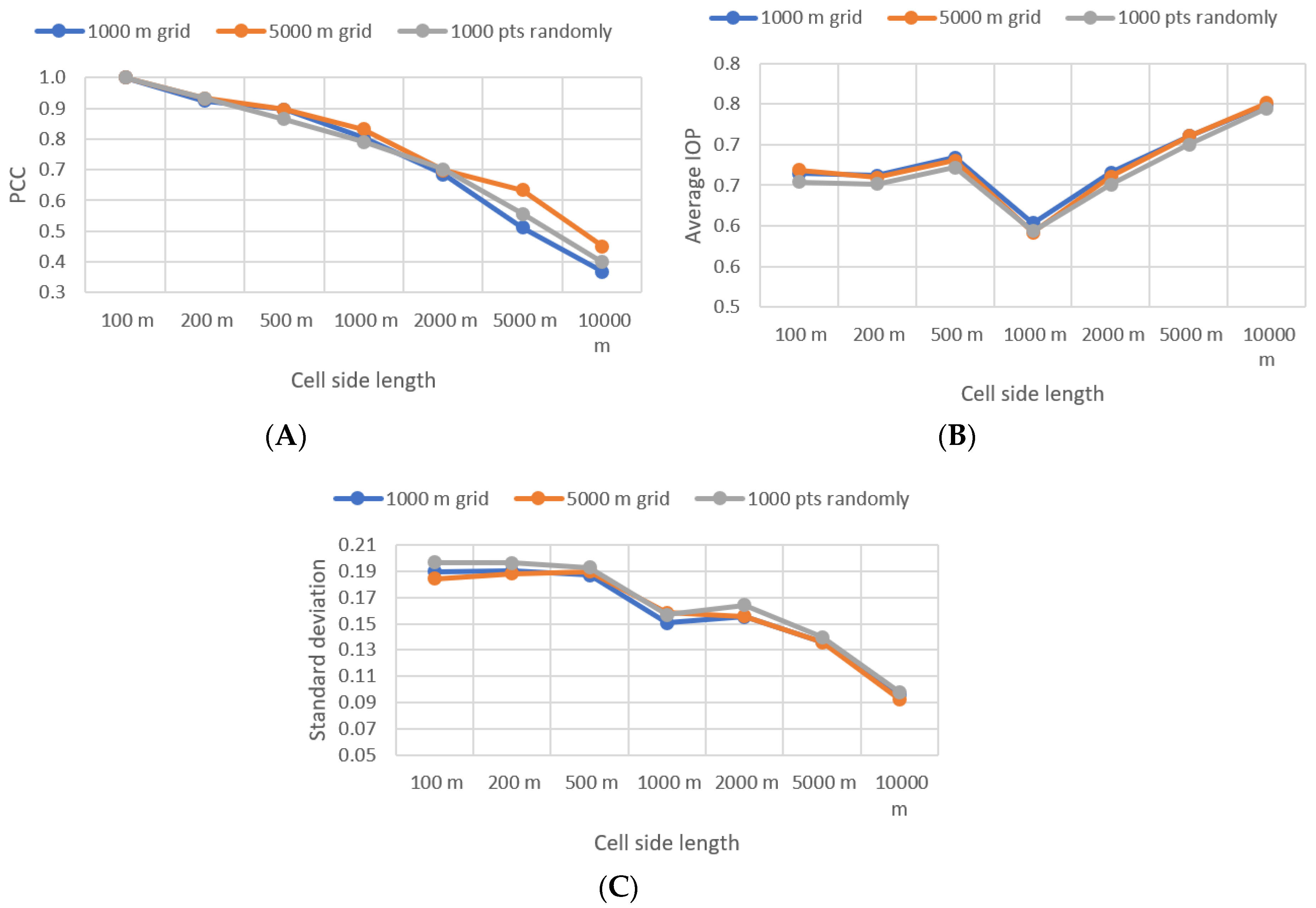
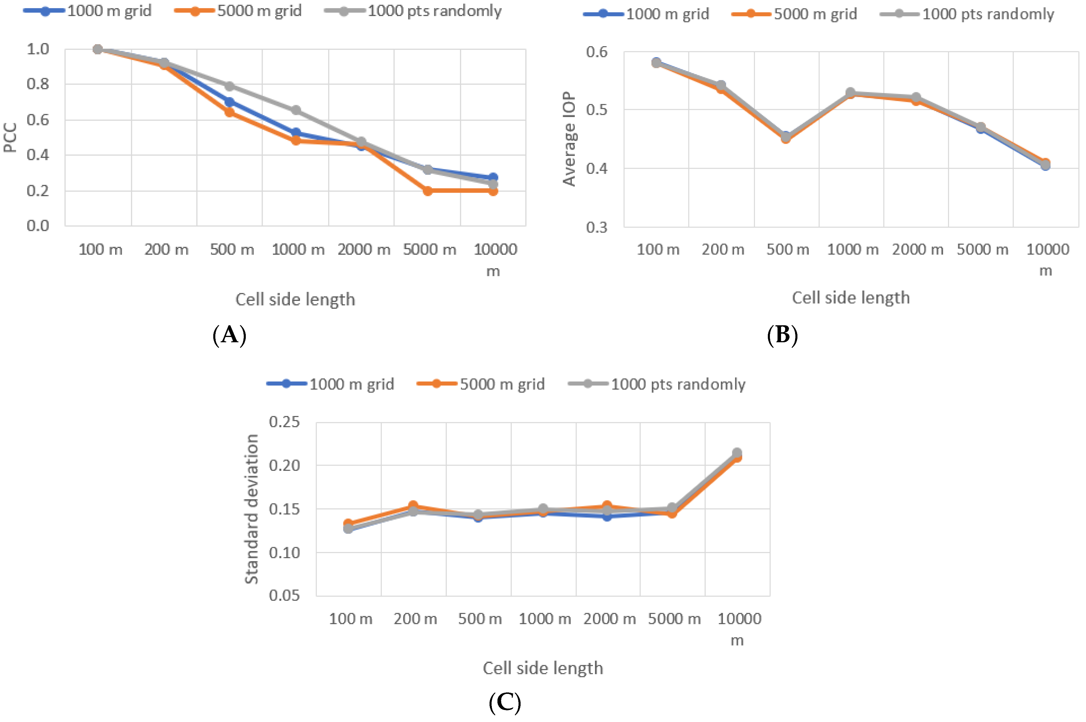
In order to facilitate the interpretation of the obtained results, figures presenting the correlations between the statistical parameters of the distribution of indices of passability were created for various sizes of cells (Figure 15). Figure 15A demonstrates clearly that the correlation between the determined indices of passability decreases with the increasing cell size. This decrease is linear and the correlation that may be treated as a measure of similarity between the maps is very low for maps generated from 100 m and 10,000 m squares (approximately 0.4). This proves that these are completely different maps, although they were created with the use of the same data and of an identical method of calculating the index of passability. Figure 15B demonstrates that the average index of passability increases with the increasing cell size. The figure shows a noticeable drop (decrease) in this average value for the 1000 m cell. It results from the fact that, starting from this cell size, the degree of generalisation, manifested as the decrease of the number of distinguishable details on the map, decreases considerably (radically). This means that this cell size is a “generalisation threshold” that separates detailed maps that contain a large number of terrain features from generalised maps.

The fact that more terrain details are noticeable on maps with a lower cell size is proven by Figure 15C, which presents a visualisation of the decreasing value of the IOP standard deviation with the increasing cell size. This estimator, being a measure of the value divergence, decreases in a near-linear progress, which means that the indices of passability become less differentiated as the size of the cell increases. This means that the differentiation of IOP in maps generated with use of a large cell size will be lower.

In the histograms (Figure 9, Figure 10 and Figure 11) generated for small cell sizes (100, 200 and 500 m), there is a noticeable increase in the number of squares with indices of approximately 0.85. Most of these cells illustrate the course of roads, which disappear on maps generated with the use of a larger cell size. For smaller squares (side length up to 500 m), the increasing number of cells with a low passability coefficient (approximately 0.25) is also noticeable. These are the impassable areas, such as forests or waters. They also disappear with the increase in cell size. The fact that larger cell sizes (2000 m, 5000 m, and 10,000 m) contain a large number of terrain objects results in higher generalisation and a noticeable “shift” of the histograms towards higher IOP.

4.3. Comparison of the Generated Passability Maps with Maps Created with Use of Analogue Methods

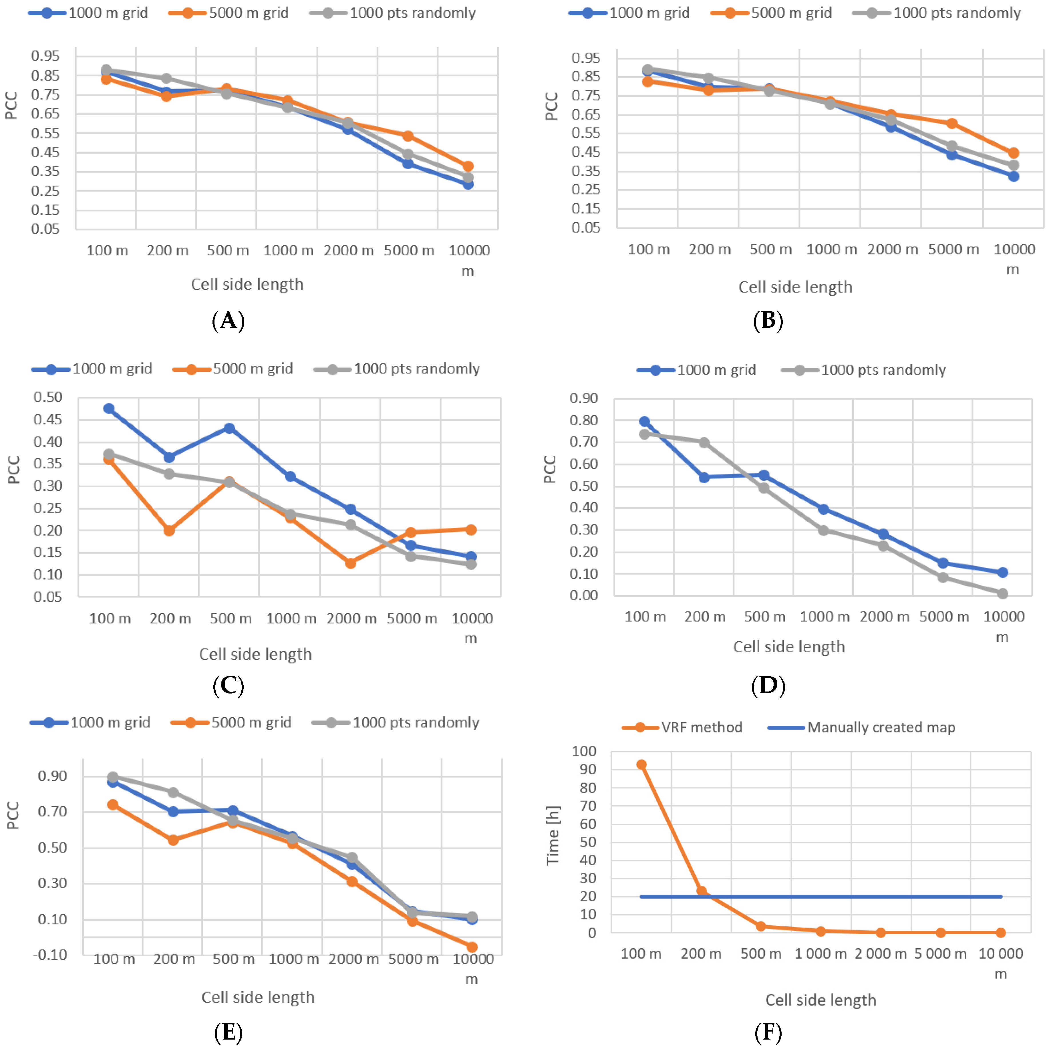
The results of the comparison of the manually generated passability map with maps generated with the use of the VRF method (Table 10, Table 11 and Table 12) clearly demonstrate that these maps are more similar, the lower the size of the cell. This is particularly noticeable for 100 and 200 m cell sizes, for which the IOP correlation coefficient exceeds 0.8. As the cell size increases, this coefficient drops in a linear way, finally reaching the value of 0.3–0.5 for maps generated for very large cell sizes (side length 5 and 10 km) (Figure 16A). The increasing divergence (decreasing PCC) is caused by the growing generalisation of the obtained passability level, which progresses with the increase in cell size. A similar situation has been noted for passability maps generated taking into account selected categories of spatial features (vegetation—Figure 16B, buildings—Figure 16D, and hydrography—Figure 16E). As far as relief is concerned (Figure 16C), the PCC between the manually created map and the map generated with the use of VRF is low (0.3–0.4), even for small cell sizes (100 and 200 m). This is because of the different methods of determining passability in terms of terrain relief. On manually created maps, impassable areas are determined with the use of thresholds, based on the sloping map (e.g., sloping exceeding 5° is a SLOW GO area), while the VRF method always takes into account the average sloping for each cell.

The results of tests consisting of the placement of control points on maps demonstrate that the passability model presented in maps generated with use of the VRF method corresponds to a large extent to maps created manually by an experienced operator. This is proven by the high correlation coefficient between those maps. It applies in particular to maps with cell size up to 1000 m, for which the correlation coefficient of the total IOP exceeds 0.75. For larger cell sizes, the map generalisation degree increases, which enables and facilitates their use by commanding officers on higher levels of command. One should also note the obvious advantage of generating passability maps with the use of the VRF method. When this method is used, the IOP is determined separately for each cell, which enables it to take into account even the smallest terrain obstacles (especially for small cell sizes). Moreover, the analysis covers all terrain features included in the VMap Level 2 conceptual model. As far as traditional (manually created) maps are concerned, they are created by marking areas of specific passability (NO GO, SLOW GO) in a binary way. Their detailedness depends on the available time and the experience of the operator.

Another argument in favour of the method based on VRF indices is the comparison of map generating time. While the creation of the most detailed map, with a 100 by 100 m cell, lasts for over two days, for maps based on 200-m squares, the time of generation becomes equal to that of creating the map of the Suwałki Pass manually. For larger cell sizes, this time becomes several times shorter than that for the tedious process of creating maps with the use of traditional methods (Figure 16F).

The results of the conducted tests also allow us to draw certain conclusions concerning the number of control points, which allows for a proper verification of differences between maps. All of the figures contained herein clearly demonstrate that, regardless of the number and configuration of control points, the obtained values are very similar. This demonstrates that it is not necessary to place a huge number of points on the map, as representative results are obtained already for a grid of a 5000-m mesh (117 points on the tested area). The two other configurations (1000-m grid—2942 points and 1000 randomly distributed points) provide very similar results that allow us to draw similar conclusions.

4.4. Evaluation of the Correctness of the Adopted Solutions

The conducted tests concerning the development of passability maps in areas other than the Suwałki Pass with the use of the OpenStreetMap database demonstrated that the presented methodology is universally applicable. The obtained maps provide the ability to distinguish areas of different passability and to draw avenues of approach of the parameters defined in Table 3, as shown in Figure 13. Similar to in the case of maps generated for the Suwałki Pass Region, the level of detail of the developed maps depends on the applied cell size.

As for the previously presented results, diagrams of correlations between the statistical characteristics of the distribution of indices of passability were created, in order to facilitate their interpretation. Figure 17A demonstrates clearly that the correlation between the determined indices of passability decreases with the increasing cell size. This is a linear decrease. This correlation is similar to that presented in Figure 15A, which illustrates the changes in the correlation coefficient for maps developed for the Suwałki Pass area. The diagram of changes in the arithmetic average, presented in Figure 17B, also proves the existence of a “generalisation threshold” in maps generated with the use of OpenStreetMap data. However, this time it occurs at the 500 m cell size, while for maps generated with use of VMap Level 2, this value was 1000 m. This is because of the fact that the used OSM (Open Street Map) database has a higher level of detail.

5. Conclusions

The presented test results enabled us to find and document the answers to the research questions posed in the introduction. The cell shape analysis confirms that the selected shape (provided that the same surface area is maintained) does not have a significant influence on the resulting passability maps. As a result, the used cell shape may be selected freely. Hence, the square cell is usually used, as it is the most convenient and least complicated shape.

The tests also enabled the authors to present a proposed selection of cell size depending on the scale of the resulting map, and thus on its designation. The results of research conducted on the other area and with use of another dataset confirm the universality of the proposed method. Therefore, the test results may be used to develop passability maps on various levels of military command. It is worth noting that the application of the automatic terrain classification method and calculating the index of passability automatically provides some indications that the whole process of creating such maps may be automated. This is the additional value of the conducted works that adds an important practical aspect to the obtained results.

It might be worth testing the obtained results, as well as the automation of the map development process, in the territories of other countries, and on terrains with different land cover features specificity. This would enable us to analyse whether the proposed solutions are universal and, as a consequence, to develop uniform solutions that would be applicable in the territories of all NATO Member States. This will be the direction of further research.

Another important conclusion from the conducted tests is the fact that maps generated automatically do not differ considerably from maps created manually by humans. The similarity is the highest for small cell sizes (100 and 200 m). This means that passability maps generated with use of the VRF method may replace traditional, manually created maps, saving many hours of work of a qualified operator. Finally, one cannot neglect the fact that maps generated with use of the presented method offer more possibilities of interpreting the terrain situation, as they present passability with use of the index expressed within the continuous range from 0 to 1, while on traditional maps, passability is determined only with use of three classes: GO, SLOW GO, and NO GO.

References

- Stöckl, R. Die Bevölkerungsdichte und verwandte Begriffe. Petermanns Geogr. Mitt. 1952, 96, 168–179. [Google Scholar]
- Andrienko, G.; Andrienko, N. Grid data analysis in the CommonGIS system: An example from forestry. In Maps and the Internet 2002; Institute of Cartography and Geomedia Technique: Vienna, Austria, 2002; pp. 89–99. [Google Scholar]
- Batista e Silva, F.; Gallego, J.; Lavalle, C. A high-resolution population grid map for Europe. J. Maps 2013, 9, 16–28. [Google Scholar] [CrossRef] [Green Version]
- Zhou, M.; Tian, J.; Xiong, F.; Wang, R. Point grid map: A new type of thematic map for statistical data associated with geographic points. Cartogr. Geogr. Inf. Sci. 2017, 44, 374–389. [Google Scholar] [CrossRef]
- Bormann, H. Effects of grid size and aggregation on regional scale landuse scenario calculations using SVAT schemes. Adv. Geosci. 2006, 9, 45–52. [Google Scholar] [CrossRef]
- Farajalla, N.; Vieux, B. Capturing the Essential Spatial Variability in Distributed Hydrological Modeling—Infiltration Parameters. Hydrol. Process. 1995, 9, 55–68. [Google Scholar] [CrossRef]
- Pelgrum, H. Spatial Aggregation of Land Surface Characteristics: Impact of Resolution of Remote Sensing Data on Land Surface Modelling; Wageningen Universiteit: Wageningen, The Netherlands, 2000; ISBN 90-5808-243-1. [Google Scholar]
- Andrienko, G.; Andrienko, N.; Gitis, V.; Denissovitch, I. Interactive Maps for Visual Exploration of Grid Data. Int. Arch. Photogramm. Remote Sens. 2001, 34, 6–9. [Google Scholar]
- Andrienko, G.; Andrienko, N.; Gitis, V. Interactive maps for visual exploration of grid and vector geodata. ISPRS J. Photogramm. Remote Sens. 2003, 57, 380–389. [Google Scholar] [CrossRef]
- Andrienko, G.; Andrienko, N.; Denisovich, I. Dynamic aggregation on grids for interactive analysis of multidimensional spatial information. In Proceedings of the 7th AGILE Conference on Geographic Information Science, Heraklion, Greece, 29 April–1 May 2004; pp. 207–212. [Google Scholar]
- Borkowski, A.; Meier, S. A procedure for estimating the grid cell size of digital terrain models derived from topographic maps. Geo-Inf. Syst. 1994, 7, 2–5. [Google Scholar]
- Florinsky, I.V.; Kuryakova, G.A. Determination of grid size for digital terrain modelling in landscape investigations—Exemplified by soil moisture distribution at a micro-scale. Int. J. Geogr. Inf. Sci. 2000, 14, 815–832. [Google Scholar] [CrossRef]
- Garbrecht, J.; Martz, L. Grid Size Dependency of Parameters Extracted from Digital Elevation Models. Comput. Geosci. 1994, 20, 85–87. [Google Scholar] [CrossRef]
- Ziadat, F.M. Effect of Contour Intervals and Grid Cell Size on the Accuracy of DEMs and Slope Derivatives. Trans. GIS 2007, 11, 67–81. [Google Scholar] [CrossRef]
- Hengl, T. Finding the right pixel size. Comput. Geosci. 2006, 32, 1283–1298. [Google Scholar] [CrossRef]
- Usul, N.; Pasaogullari, O. Effect of Map Scale and Grid Size for Hydrological Modelling; GIS and Remote Sensing in Hydrology, Water Resources and Environment. In Proceedings of the International Conference on GIS and Remote Sensing in Hydrology, Water Resources and Environment (ICGRHWE), Three Gorges Dam, Yichang, China, 16–19 September 2003; pp. 91–100. [Google Scholar]
- Moscicka, A.; Pokonieczny, K.; Tomala, J. Selection of Optimal Measurement Point Density in Travel Time Mapping: Warsaw Airport Case Study. In Proceedings of the 2016 Baltic Geodetic Congress (BGC Geomatics), Gdańsk, Poland, 2–4 June 2016; pp. 211–216. [Google Scholar] [CrossRef]
- Field Manual 5-33 Terrain Analysis; Department of US Army: Washington, DC, USA, 1990.
- NO-06-A015:2012, Terrain—Rules of Classification—Terrain Analysis on Operational Level; Polish Ministry of National Defence: Warsaw, Poland, 2012.
- Pokonieczny, K. Automatic military passability map generation system. In Proceedings of the 2017 International Conference on Military Technologies (ICMT), Brno, Czech Republic, 31 May–2 June 2017; pp. 285–292. [Google Scholar] [CrossRef]
- Campbell, L.; Lotwin, A.; DeRico, M.M.G.; Ray, C. The use of Artificial Intelligence in military simulations. In Proceedings of the 1997 IEEE International Conference on Systems, Man, and Cybernetics. Computational Cybernetics and Simulation, Orlando, FL, USA, 12–15 October 1997; pp. 2607–2612. [Google Scholar]
- Miller, D.; Rueter, S. Mission Specific Terrain Analysis. Google Patent No. US20130035861A1, 7 February 2013. [Google Scholar]
- Glinton, R.; Giampapa, J.; Owens, S.; Sycara, K.; Grindle, C.; Lewis, M. Integrating context for information fusion: Automating intelligence preparation of the battlefield. In Human Performance, Situation Awareness and Automation: Current Research and Trends, Proceedings of the 2nd Conference on Human Performance, Situation Awareness and Automation (HPSAA II), Daytona Beach, FL, USA, 22–25 March 2004; Vincenzi, D.A., Mouloua, M., Hancock, P.A., Eds.; Lawrence Erlbaum Associates: Mahwah, NJ, USA, 2004; pp. 224–229. [Google Scholar]
- Lee, S.; An, H.; Yu, S.; Oh, J.J. Creating an advanced backpropagation neural network toolbox within GIS software. Environ. Earth Sci. 2014, 72, 3111–3128. [Google Scholar] [CrossRef]
- Richbourg, R.; Olson, W.K. A hybrid expert system that combines technologies to address the problem of military terrain analysis. Expert Syst. Appl. 1996, 11, 207–225. [Google Scholar] [CrossRef]
- Hošková-Mayerová, Š. Geospatial Data Reliability, Their Use in Crisis Situations. In Proceedings of the International Conference KNOWLEDGE-BASED ORGANIZATION, Sibiu, Romania, 11–13 June 2015; pp. 694–698. [Google Scholar] [CrossRef]
- Jayakumar, P.; Mechergui, D.; Wasfy, T.M. Understanding the Effects of Soil Characteristics on Mobility. In Proceedings of the ASME 13th International Conference on Multibody Systems, Nonlinear Dynamics, and Control, Cleveland, OH, USA, 6–9 August 2017. [Google Scholar] [CrossRef]
- Pokonieczny, K.; Wyszyński, M. Automation of the terrain assessment classification due to passability for the needs of crisis managment. In Proceedings of the 16th International Multidisciplinary Scientific GeoConference & EXPO SGEM2016, Albena, Bulgaria, 28 June–7 July 2016; pp. 119–126. [Google Scholar] [CrossRef]
- Hubacek, M.; Ceplova, L.; Brenova, M.; Mikita, T.; Zerzan, P. Analysis of vehicle movement possibilities in terrain covered by vegetation. In Proceedings of the International Conference on Military Technologies (ICMT), Brno, Czech Republic, 19–21 May 2015; pp. 1–5. [Google Scholar] [CrossRef]
- Rybansky, M. Trafficability analysis through vegetation. In Proceedings of the 2017 International Conference on Military Technologies (ICMT), Brno, Czech Republic, 31 May–2 June 2017; pp. 207–210. [Google Scholar] [CrossRef]
- Svendsen, N.G.; Koch, D.J.; Gertner, G.Z.; Howard, H.R.; Ayers, P.D. Vehicle Impact Analysis Using Vehicle Tracking Systems on Military Lands. Trans. ASABE 2017, 60, 1865–1872. [Google Scholar] [CrossRef]
- Pokonieczny, K. Methods of Using Self-organising Maps for Terrain Classification, Using an Example of Developing a Military Passability Map. In Dynamics in GIscience; Lecture Notes in Geoinformation and Cartography; Springer: Cham, Switzerland, 2017; pp. 359–371. [Google Scholar]
- Rybansky, M.; Hofmann, A.; Hubacek, M.; Kovarik, V.; Talhofer, V. Modelling of cross-country transport in raster format. Environ. Earth Sci. 2015, 74, 7049–7058. [Google Scholar] [CrossRef]
- Hofmann, A.; Hošková-Mayerová, Š.; Talhofer, V.; Kovařík, V. Creation of models for calculation of coefficients of terrain passability. Qual. Quant. 2014, 49, 1679–1691. [Google Scholar] [CrossRef]
- Gotlib, D.; Iwaniak, A.; Olszewski, R. GIS Obszary Zastosowania (GIS Application Areas); Wydawnictwo Naukowe PWN: Warsaw, Poland, 2007; ISBN 978-83-01-15354-0. [Google Scholar]
- Pokonieczny, K.; Rybansky, M. Method of developing the maps of passability for unmanned ground vehicles. In Proceedings of the 9th IGRSM International Conference and Exhibition on Geospatial & Remote Sensing, Kuala Lumpur, Malaysia, 24–25 April 2018. [Google Scholar]
- Military Specification MIL-V-89032 Vector Smart Map (VMAP) Level 2; National Imagery and Spatial Agency: Washington, DC, USA, 1993.
- Farr, T.G.; Rosen, P.A.; Caro, E.; Crippen, R.; Duren, R.; Hensley, S.; Kobrick, M.; Paller, M.; Rodriguez, E.; Roth, L.; et al. The Shuttle Radar Topography Mission. Rev. Geophys. 2007, 45. [Google Scholar] [CrossRef] [Green Version]
- Elak, L.; Śliwa, Z. The Suwalki gap—NATO’s fragile hot spot. Zeszyty Naukowe AON 2016, 103, 24–40. [Google Scholar]
- Field Manual 34-130 Intelligence Preparation of the Battlefield; Department of US Army: Washington, DC, USA, 1994.
- STANAG 2259, ED. 4: Military Geographic Documentation—Terrain; Department of US Army: Washington, DC, USA, 1975.
- Larose, D.T. Data Mining Methods and Models; John Wiley & Sons, Inc.: Hoboken, NJ, USA, 2006; ISBN 978-0-471-75648-4. [Google Scholar]
- Fisher, R.A. The general sampling distribution of the multiple correlation coefficient. Proc. R. Soc. Lond. A 1928, 121, 654–673. [Google Scholar] [CrossRef]
Figure 1.
An example of selected parameters for a cell.
Figure 2.
Test areas (left side—cell shape analysis, right side—cell size analysis). NATO—North Atlantic Treaty Organization.
Figure 3.
Topographic map of test area, source: © OpenStreetMap contributors.
Figure 4.
Manner of distribution of control points (analysis of the shape of cells).
Figure 5.
Manner of distribution of control points (analysis of the size of cells).
Figure 6.
The area where the universality of solutions was tested, source: © OpenStreetMap contributors.
Figure 7.
Fragments of passability maps generated for cells of a surface area of 1 km2 and different shapes.
Figure 8.
Fragments of passability maps for various sizes of cell. IOP—indices of passability.
Figure 9.
Histogram of the distribution of indices of passability for the analysed cell sizes for the 1000 m control point grid (2942 points).
Figure 10.
Histogram of the distribution of indices of passability for the analysed cell sizes for the 5000 m control point grid (117 points).
Figure 11.
Histogram of the distribution of indices of passability for the analysed cell sizes for 1000 randomly distributed control points.
Figure 12.
Fragments of a military passability map divided into topical categories of content elements.
Figure 13.
Parts of passability maps for various sizes of cell generated for the area of the Warsaw Agglomeration.
Figure 14.
Fragments of passability maps generated for the largest cells in the whole test area.
Figure 15.
Correlation between the values of statistical parameters and cell size. (A) Correlation between PCC and cell size (for 100 m fields); (B) Correlation between average IOP and cell size; (C) Correlation between standard deviation and cell size.
Figure 16.
Correlation between the values of statistical parameters and cell size. (A) Correlation between PCC and cell size in terms of total IOP; (B) Correlation between PCC and cell size in terms of vegetation; (C) Correlation between PCC and cell size in terms of relief; (D) Correlation between PCC and cell size in terms of buildings; (E) Correlation between PCC and cell size in terms of hydrography; (F) Correlation between map generating time and cell size.
Figure 17.
Correlation between the values of statistical parameters and cell size for test area. (A) Correlation between PCC and cell size (for 100 m fields) for test area; (B) Correlation between average IOP and cell size for test area; (C) Correlation between standard deviation and cell size for test area.