Article

The Classification of Noise-Afflicted Remotely Sensed Data Using Three Machine-Learning Techniques: Effect of Different Levels and Types of Noise on Accuracy

1
University of the Chinese Academy of Sciences, Beijing 100094, China
2
State Key Laboratory of Remote Sensing Science, Institute of Remote Sensing and Digital Earth, Chinese Academy of Sciences, Beijing 100101, China
*
Author to whom correspondence should be addressed.
ISPRS Int. J. Geo-Inf. 2018, 7(7), 274; https://doi.org/10.3390/ijgi7070274
Submission received: 8 May 2018 / Revised: 12 June 2018 / Accepted: 26 June 2018 / Published: 12 July 2018

Abstract

:
Remotely sensed data are often adversely affected by many types of noise, which influences the classification result. Supervised machine-learning (ML) classifiers such as random forest (RF), support vector machine (SVM), and back-propagation neural network (BPNN) are broadly reported to improve robustness against noise. However, only a few comparative studies that may help investigate this robustness have been reported. An important contribution, going beyond previous studies, is that we perform the analyses by employing the most well-known and broadly implemented packages of the three classifiers and control their settings to represent users’ actual applications. This facilitates an understanding of the extent to which the noise types and levels in remotely sensed data impact classification accuracy using ML classifiers. By using those implementations, we classified the land cover data from a satellite image that was separately afflicted by seven-level zero-mean Gaussian, salt–pepper, and speckle noise. The modeling data and features were strictly controlled. Finally, we discussed how each noise type affects the accuracy obtained from each classifier and the robustness of the classifiers to noise in the data. This may enhance our understanding of the relationship between noises, the supervised ML classifiers, and remotely sensed data.

Graphical Abstract

1. Introduction

Remotely sensed data, especially for satellite images, are used to estimate information about the Earth, its various objects, phenomena, and processes. These images have been widely used for applications of Earth surface monitoring such as land cover classification and change detection, crop yield estimation, and geographic information extraction. Improving the accuracy of the classifications is thus a fundamental research topic in the field of geographic information sciences [1]. However, it can be a difficult task depending on the complexity of the landscape, the spatial and spectral resolution of the imagery being used, and the amount of noise included.
Noise may be added to remotely sensed data during different stages of data acquisition or processing, from the moment the data are captured by the sensor until their atmospheric and topographic correction, orthorectification, or co-registration [2]. In satellite image classification, the data obtained from the satellite sensors may be affected by atmospheric noise resulting from the obstruction of the light reflected by targets on the Earth’s surface by a variety of phenomena, including aerosols and clouds in the atmosphere as well as changing illumination patterns and the angle at which the satellite views the ground at any given time [3]. The basic source for image pixels, such as those acquired by satellite sensors, has limited radiometric and geometric resolution. This effect leads to a mixture of classes within one pixel, thereby resulting in the representation of the partial degree membership of at least two classes in the pixel, known as a mixed pixel, which normally increases the classification complexity [4]. Moreover, the image generation process may add noise to the data. This is widely found in most Synthetic-aperture radar (SAR) images [5,6,7]. These data have to be compressed to reduce their requirements for archiving and data transmission and this may cause artifacts and ambiguities in the final images [8].
Normally, the normal distribution values that occur at a random location by merging with the original values in the satellite image are referred to as zero-mean Gaussian noise [9]. In optical remote sensing multispectral imagery, the noise is typically independent of the data and it is generally additive in nature. The noise may reduce the performances of important techniques of image processing such as detection, segmentation, and classification. Most of the natural images are assumed to have additive white Gaussian noise [10,11].
Salt and pepper noise are the highest and lowest global values, respectively, that replace an original pixel at a random location. This is generally caused due to errors in data transmission [5,12]. A report of data loss on the Landsat Missions website also refers to an artifact called Christmas Tree anomaly. The lost data appear as bright red, green, and blue artifacts, often next to or overlapping each other. This artifact is usually caused by telemetry data erroneously being included in the satellite imagery [13]. The missing data may be replaced by null values (salt noise) or filled with a designated fill pattern by the ground processing systems. Charoenjit et al. [14] stated that one of the problems associated with biomass estimation from very high-resolution (VHR) data is salt–pepper noise. In an attempt to solve the problem caused by the noise, these authors performed object-based image analysis on a Para rubber plantation and proved that the segmentation method can reduce the effect of constant salt–pepper noise.
Multiplicative noise or speckle is widely found in most SAR images [5,6,7]. These data have to be compressed to reduce their requirements for archiving and data transmission and this may cause artifacts and ambiguities in the final images [8,15]. Speckle noise gives a grainy appearance to radar imageries. It reduces the image contrast, which has a direct negative effect on the texture-based analysis of the imageries [16,17]. For example, Nobrega et al. [18] showed a LiDAR intensity image that was affected by signal eccentricities caused by sensor scanning patterns. By filtering the noise, they could improve the efficiency of the image’s segmentation. Moreover, Mulder et al. [19] reviewed the use of remotely sensed data for soil and terrain mapping. They concluded that the accuracy of retrieving soil information by using proximal sensing combined with a remote sensing method decreases because of several types of noise such as that caused by a mixture of soil properties and atmospheric, topographic, and sensor noise. Soil moisture retrieval from SAR images is always affected by speckle noise and uncertainties associated with soil parameters, which impact negatively the accuracy of soil moisture estimates. Barber et al. [7] proposed a soil moisture Bayesian estimator from polarimetric SAR images to address these issues. The results indicated that the model enlarges the validity region of the minimization-based procedure and the speckle effects can be reduced by the multilooking method included in the model scheme.
Consequently, the effect of noise within the data can be either mitigated or ignored by selecting appropriate classifiers that are robust to noise, especially for supervised machine-learning classifiers which have a mechanism for handling noise [20,21,22,23]. Continuous developments in storage capacity and the processing speed of computers made advanced machine learning (ML) available for land cover classification. Supervised machine-learning algorithms require external assistance in the form of training [24]. Their classification accuracy obviously depends on the quality of the training data [20]. The input dataset is normally divided into training and testing datasets. The training dataset has an output variable that needs to be predicted or classified. Most algorithms learn some kind of pattern from the training dataset and apply them to the test dataset for prediction or classification [25,26].
Algorithms based on random forests (RF) [21] utilize decision trees. These algorithms are probably one of the most efficient ML algorithms in terms of prediction accuracy [27]. The algorithm has the capability to rapidly process databases ranging from small to very large, and is easy to interpret and visualize [28]. Moreover, RF has been reported to be robust to noise [29,30,31]. However, the algorithm can slow down as the number of trees increases [28]. In recent decades, many scientists have used RF as a classifier. In the original paper describing RF [21], the performance of RF was observed against Adaboost algorithms [32] by classifying 20 different datasets. The authors proved that RF is more robust with respect to noise. Moreover, Crisci et al. [27] reviewed a number of supervised ML algorithms to model mortality events in benthic communities in rocky coastal areas in the northwestern Mediterranean Sea. The RF model yielded the lowest misclassification rates for such ecological data.
Support vector machine (SVM) is a supervised non-parametric statistical learning technique; therefore, no assumption is made about the underlying data distribution [33]. The SVM learning algorithm aims to find a hyperplane that separates the dataset into a discrete predefined number of classes in a fashion consistent with the training examples. SVM outperforms other ML models, particularly when only a small dataset is available for training [34,35]. However, SVM requires more training time and its performance is dependent on parameter adjustment in comparison to other methods [23]. For classification purposes, Dalponte et al. [36] used SVM and the fusion of hyperspectral and LiDAR data, in which speckle noise usually existed. They pointed out that SVM outperformed the maximum likelihood and k-nearest neighbor (k-NN) techniques. Moreover, the incorporation of LiDAR variables generally improved the classification performance and the first return data was the highest contributing factor. Insom et al. [34] improved the accuracy of standard SVM by applying a particle filter (PF) to automatically update the SVM training model parameters to values that were more appropriate for their flood dataset. The performance of the method is superior when compared with standard SVM. Senf et al. [37] performed land cover classification of complex Mediterranean landscapes using an SVM classifier. The work proved that combining phonological profiles of the land covers and human interpretation can significantly improve the generalization power of the SVM models, as previously stated [38]. Moreover, SVM was also reported to have good generalization capabilities under different noise levels, types of noise, and sample sizes when it was optimized [39].
A neural network (NN) is an algorithm that simulates the neuronal structure, processing method, and learning ability of the human brain but on much smaller scales. This technique is applicable to problems in which the relationships may be nonlinear or quite dynamic [40]. The most common type of NN is based on the back-propagation learning algorithm and is known as a back-propagation neural network (BPNN) [41]. BPNN has been proven to be the best among the Multi-layer perceptron (MLP) algorithms [22]. However, BPNN tends to be slower to train than other types of NNs, which can be problematic in very large networks with a large amount of data [28]. BPNNs in remotely sensed image classification applications have been widely reviewed [41,42,43]. They were also reported as very effective to use in noise reduction [44,45] and robust to noises when trained by noise data [46]. These researchers have mutually concluded that the BPNN approach is feasible for the classification of remote sensing imagery.
In recent decades, many experiments have been designed for studies aiming to observe the robustness of a variety of classifiers relating to noise content and type. For example, Petrou et al. [2] proposed fuzzy-rule-based classifiers to overcome uncertainty in habitat mapping. The robustness of these classifiers was evaluated by drawing additive homogeneous noise from a zero-mean Gaussian probability density function. The noise was added to the original images and a threshold was assigned by an expert at different standard deviations ranging from 5 to 20% of the image mean values and 5 to 50% of the rule threshold, respectively. The results showed that the classifiers remained mostly unaffected by noise in the data that were used because the classification was object based. In contrast, the additive noise in the rule threshold, which acted as inaccurate expert rules, directly affected the performance. However, the overall accuracies remained over 75%. Celik and Ma [9] investigated the performance of their automatic change-detection method by using different types and levels of added noise. Different levels of zero-mean Gaussian noise ranging from 35 to 50 dB (peak signal-to-noise ratio (PSNR)) were used in the experiments. Moreover, the authors contaminated the test images with different levels of speckle noise to illustrate the noise that commonly occurs in SAR data. The method proved to be highly robust (accuracies of approximately 95–100%) to both types of noise when the classifier was assigned an appropriate parameter value. Moreover, the noise test could assist the authors in optimizing the parameter used in the classification with different levels of noise. Dierking and Dall [6] used complex scattering matrix data of the Electromagnetics Institute’s Synthetic Aperture Radar (EMISAR) system in order to simulate image products with different levels of pixel dimensions and noise levels of −35, −30, −25, and −20 dB. Ice deformation maps were generated by using a selected threshold, such that image pixels with intensities equal to or larger than the highest 2% of the ice intensity distribution level were classified as deformed ice. The results indicated that if the level of the sensor noise is equal to or larger than the average backscattering intensity of the level ice, the retrieved values for the deformation parameters change. Moreover, an L-band SAR system at like-polarization, with an incidence angle larger than 35° and a noise level of at most −25 dB or lower, is desirable for mapping the deformation state of sea ice cover.
In this work, we employed three supervised ML classifiers, i.e., random forest (RF), support vector machine (SVM), and back-propagation neural network (BPNN), to classify the land covers in satellite images afflicted by three classes of noise, namely zero-mean Gaussian, salt–pepper, and speckle noise. The classification was first carried out on an image corrected for absolute atmospheric interference, termed the reference image, to obtain the standard accuracies. Subsequently, noise was applied to the reference image in different concentrations. The normal reflectance image (without absolute atmospheric correction) was also classified to illustrate the real effects of mixing different kinds of noise. To conclude, we experimented with the performance of the classifiers under the following noise conditions:
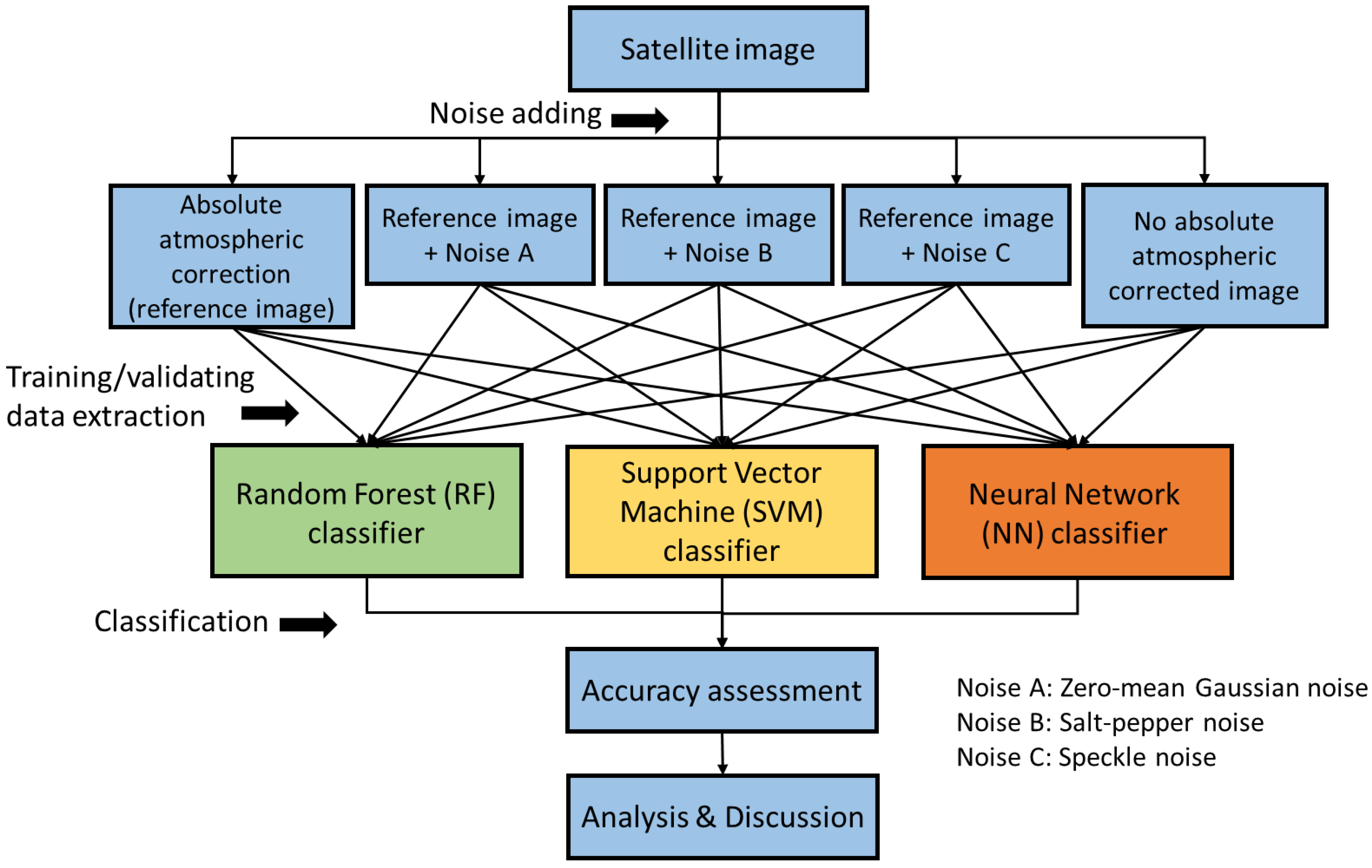
  • Fully processed images with absolute atmospheric correction, termed the reference images. (assumed to contain no noise);
  • Normal reflectance images without absolute atmospheric correction (mixture of noise, i.e., sensor noise, atmospheric noise);
  • Reference images with zero-mean Gaussian noise added;
  • Reference images with salt–pepper noise added;
  • Reference images with speckle noise added (multiplicative noise).
Discussions are presented to describe and examine the performance of the different classifiers to each noise type and level in addition to assessing the research questions: (1) To what extent do the different types of noise affect the classification accuracies? (2) How do the classifiers behave toward noise-afflicted image classification? Additionally, the effect of the different types of noise and the behavior of the classifiers on remotely sensed data are considered. Note that the results and conclusions that we made in this study are mainly aimed at providing an understanding of the core mechanisms of the ML classifiers toward noises in remotely sensed data rather than comparing their performances.

2. Materials and Methods

2.1. Experimental Design

Figure 1 shows the overall experimental flow of the current study. A Landsat 8 OLI scene was acquired and processed to be a reference image (refer to Section 2.2. for the image processing). We added different levels of three types of noise, zero-mean Gaussian noise, salt–pepper noise, and speckle noise to the reference image to produce noise-afflicted images. Twenty-three images (one reference image, one image without absolute atmospheric correction, and 21 images to which artificial noise was added) were then classified by BPNN, SVM, and RF to obtain the classification accuracies. The classifications were scoped by the following conditions. First, the training and validating samples were extracted using the same shape file (i.e., samples were acquired at the same image locations). Second, the parameters used in each of the algorithms were optimized. Please refer to Section 2.4 for a detailed explanation. In addition, we observed the robustness of a classifier by the differential accuracies of the reference image and the images to which noise was added.

2.2. Remotely Sensed Data

The satellite image is a Landsat-8 Operational Land Imager (OLI) image acquired on 26 December 2014 (Path 130, Row 50), shown in Figure 2. The image was acquired under clear sky conditions, a very low content of homogeneous aerosol, and in the absence of cloud objects. The scene includes Landsat 8 surface reflectance data generated from the Landsat Surface Reflectance Code (LaSRC). The LaSRC makes use of the coastal aerosol band to perform aerosol inversion tests, uses auxiliary climate data from the Moderate Resolution Imaging Spectroradiometer (MODIS), and uses a unique radiative transfer model. The model artifacts or blockiness presented in the surface reflectance data products were excluded from the image and any future calculation by employing the quality assessment (QA) band. We termed this image the reference image.
The study area, which covered the southeastern part of the Srinakarin dam, an embankment dam on the Khwae Yai River in the Si Sawat District of the Kanchanaburi Province of Thailand, included five land cover classes: agriculture, bare land, construction, water body, and forest. Descriptions of the classes are provided in Table 1. The sample pixel locations were randomly selected from Thailand’s 2014 land cover ground survey map obtained from the Geo-Informatics and Space Technology Development Agency (GISTDA). The phenology of plants or land cover may change after the referencing date (the time lapse is about two months). Thus, we incorporated human interpretation and Google Earth images with an acquisition date near the Landsat image to confirm that the samples had not changed category during the time lapse.

2.3. Sampling Design

The sampling framework utilized in this paper can be explained as follows. (1) Four thousand and four hundred random samples were randomly generated based on the Thailand’s 2014 land cover ground survey map via Generate Random Sample—Using Ground Truth Classification Image in ENVI classic version 5.1. (Harris Geospatial Solutions, Inc., Melbourne, Australia) The random samples include all classes except the construction class because it rarely existed in the study area; therefore, we manually selected 100 samples of the construction class by human interpretation. The initial 4550 random samples include 2600 samples of the forest class, 650 samples of the agriculture class, 650 samples of the bare land class, and 650 samples of the water body class. Note that the forest class accounts for more than 50% land cover of the study area, so we provided a sample size three times larger than other classes to capture the forest diversity. On the other hand, we maintained the same proportion for the water body class as it has less complexity. As a result, 4650 samples were obtained in this step. (2) The samples close to the edge of the class vectors or their classes changed during the time lapse of the data acquisition and survey map and were excluded. The criterion for removing the edge’s pixels is that the distance from the vector line is less than three pixels or 90 m. The remaining pixels were compared one-by-one with the Google Earth images using human interpretation to detect any category changes. (3) Finally, 4270 samples remained in the experiment. An 80/20 ratio of training and validation samples was randomly drawn without replacement in MATLAB programing. The final sample distribution is shown in Table 1.
To ensure that the accuracy of the classifiers was comparable and less biased, 80% of data points was used to train the various classification algorithms and 20% was used for comparison. This means that all of the training elements required for generating a classification model—training set, testing set, or validating set (if needed)—were included in the 80% training data. Note that each classifier used this data in different ways based on the training algorithms. The management of the training data of each classifier can be found in Section 2.5. Finally, we distinctly preserved 854 validating samples that were sparse in the image (20% of the reference data) to evaluate the classification accuracies. Note that only the Coastal, Blue, Green, Red, Near-Infrared (NIR), Shortwave-Infrared 1 and 2 (SWIR1 and SWIR2, respectively) bands of the Landsat 8 OLI dataset were used as spectral features in this study.

2.4. Noise Afflictions

We investigated the highest case of noise affliction in the satellite image by simulating the types of noise mentioned below in the MATLAB environment, which was then applied to the reference image at different levels of noise. The Gaussian distribution noise can be expressed by:
P ( x ) = 1 / ( σ 2 π ) × e ( x μ ) 2 2 σ 2 ,
where P(x) is the Gaussian distribution noise in an image; μ and σ are the mean and standard deviation of the noise process, respectively.
Salt and pepper noise are the highest and lowest global values, respectively, that replace an original pixel at a random location. To simulate salt and pepper noise, the following conditions were applied to the noise-free image:
p ( x ) = { p 1 , x = A p 2 , x = B 0 , o t h e r w i s e ,
where p 1 and p 2 are the probabilities density function (pdf); p ( x ) is the distribution of salt and pepper noise in image; A, B are the possible minimum and maximum values, respectively (in this paper they are 0 and 1, respectively).
The speckle noise is known as multiplicative noise, i.e., it is produced by the coherent superposition of spatially random multiple scattering sources within the resolution volume of the sensor [47]. The speckle noise distribution can be expressed as:
J = I + n × I ,
where J is the distribution speckle noise image; I is the input image; and n is the uniform noise image by specific mean and variance.
The noise level is quantitatively defined in decibels (dB) in terms of the PSNR. Given an input image I and its noisy image H , the PSNR between the two images can be expressed as:
MSE = ( 1 / m n ) i = 1 m j = 1 n [ I ( i , j ) H ( i , j ) ] 2 ,
where i and j are pixel locations in rows and columns, and m and n are the maximum number of image rows and columns, respectively.
Note that a smaller value of the PSNR refers to increasing noise intensity. The noisy images were produced by using different PSNR values. Finally, the sample images used in this study comprise a total of 23 datasets with the following descriptions:
Reference images (applied absolute atmospheric correction and noise removal)
Level 1 Landsat 8 images without absolute atmospheric correction (only convert from digital number to reflectance values)
Reference images + zero-mean Gaussian noise from 10 to 40 dB (in steps of 5 dB)
Reference images + salt and pepper noise from 10 to 40 dB (in steps of 5 dB)
Reference images + speckle noise from 10 to 40 dB (in steps of 5 dB)
Note that each pixel value of the reference image was rescaled to values between 0 and 1 using the minimum and maximum values (as shown in Equation (5)) of its band before noise generation. If an image data has i rows, v columns, and u bands, the rescaling equation in this work is expressed as:
I ( i , v , u ) = ( Q ( i , v , u ) min ( u ) ) / ( max ( u ) min ( u ) ) ) ,
where I ( i , v , u ) is the rescaled value of the original value Q ( i , v , u ) . The terms min ( u ) and max ( u ) denote the minimum and maximum values selected from band u , respectively.

2.5. Classifiers—Implementation Packages

The classifiers are described in terms of their key concepts, operational details, and parameter settings that are exclusively used in this study. Further details of both the theoretical and mathematical descriptions can be found by linking to the appropriate work that provides extensive points of interest (RF: [21,48,49], SVM: [50,51], BPNN: [22,42]).

2.5.1. Random Forests (RF)

Random Forests build multiple decision trees based on random bootstrapped samples of the training data. In contrast to other classifiers, RF neither causes overfitting nor does it require a long training time [21]. Each tree is built using a subset that differs from the original training data, containing approximately two-thirds of the cases, and the nodes are split using the best split variable among a subset of m randomly selected variables [52]. The trees are created by drawing a subset of training samples by using the replacement or bagging method. Each decision tree is independently produced without any pruning and each node is split using a number (m) defined by the user. By growing the forest up to the number of trees (k), the algorithm creates trees with high variance and low bias [21]. The final classification decision is taken by averaging the class assignment probabilities calculated by all trees. Therefore, two parameters are required to construct an RF framework: the number of trees (ntree) in the ensemble and the number of variables used to split the nodes (mtry). The classifications were performed using the well-known “randomForest” package for R [43].
All of the considered parameters were investigated, namely, the ntree was observed from 500 to 2000, and the mtry was observed from 2 to 5. The resulting model was selected by choosing the most accurate model that was obtained by running the model generation procedure 30 times. Table 2 shows the parameter tuning of all classifiers in this study.

2.5.2. Support Vector Machines (SVM)

The SVM algorithm aims to find a decision boundary termed a hyperplane that separates the dataset into a discrete predefined number of classes in a fashion consistent with the training examples. In this study, we employed the well-known “LIBSVM” package [53] implemented in the MATLAB environment. A brief mathematic description of the SVM package is provided below.
Given the input training sets of l examples x i with labels y i : ( x i , y i ) , i = 1 , 2 , 3 , , l where x i R N and y { 1 , 1 } l , the SVMs require the solution of the following optimization problem [53] as revised from The Soft Margin Hyperplane [51]:
max w , b , ξ 1 2 w T w + C i = 1 i ξ i , subject   to   y i ( w T ϕ ( x i ) + b ) 1 ξ i , ξ i 0 ,
where w , b , T , and ξ are the l-dimensional vectors, bias, transpose function, and non-negative variables, respectively. The training vectors x i are mapped into a higher dimensional space by the function ϕ . SVM finds a linear separating hyperplane with the maximal margin in this higher dimensional space. C > 0 denotes the penalty parameters of the error term. Furthermore, K ( x i , x j ) ϕ ( x i ) T ϕ ( x j ) is termed the kernel function. In this work, the radial basis function (RBF) kernel is used. It is expressed as:
K ( x i , x j ) = e x p ( γ x i x j 2 ) , γ > 0 ,
where γ is the kernel parameter. Therefore, only two parameters—the penalty parameter C and kernel parameter γ —are required when using the method.
To attain reasonable accuracy in each of the classifications, we implemented the algorithm in a step-by-step manner. First, the training data were converted to a suitable form for the SVM package. The labels were changed from category attributes into binary numbers 0 and 1. For example, {water body, constructions, agriculture} were represented as (1,0,0), (0,1,0), and (0,0,1). The straightforward grid-search cross-validation approach [53], which is provided in the package, was performed to find the best model parameters, since the values of C and γ directly affect the performance of the SVM model [34]. The cross-validation was replicated 30 times (Table 2). Therefore, the final SVM model was generated by training the entire training set by the obtained parameters in regards to the testing set, after which we exported the model to classify the 20% validating data.

2.5.3. Back-Propagation Neural Network (BPNN)

The goal of BPNN is to compute the partial derivative or gradient of a loss function with respect to any weight in the network. The loss function calculates the difference between the input training example and its expected output, after the example has been propagated through the network [36]. The basic concern of an NN algorithm is that it cannot perform accurately beyond the range of trained inputs; that is, the classification accuracies strongly depend on the data used to train the networks. The modeling data were labeled by binary number forms and then they were randomly separated into training, testing, and validating sets in the ratios of 70%, 15%, and 15%, respectively. The number of hidden layers was observed from 5 to 60. The BPNN model was automatically trained until the network converges by using the trainscg function (scaled conjugate gradients or SCG), the details of which have been described by Moller [49], in the MATLAB environment. The SCG training was automatically optimized by the parameter sigma σ (which determines the change in weight for the second derivative approximation) and lamda λ (which regulates the indefiniteness of the Hessian). The values of σ and λ were taken as 5 × e−5 and 5 × e−7, respectively. The model was repeated 30 times and the best model was then employed to classify the given validating data. The mean and standard deviation of the model accuracies were reported.

3. Results

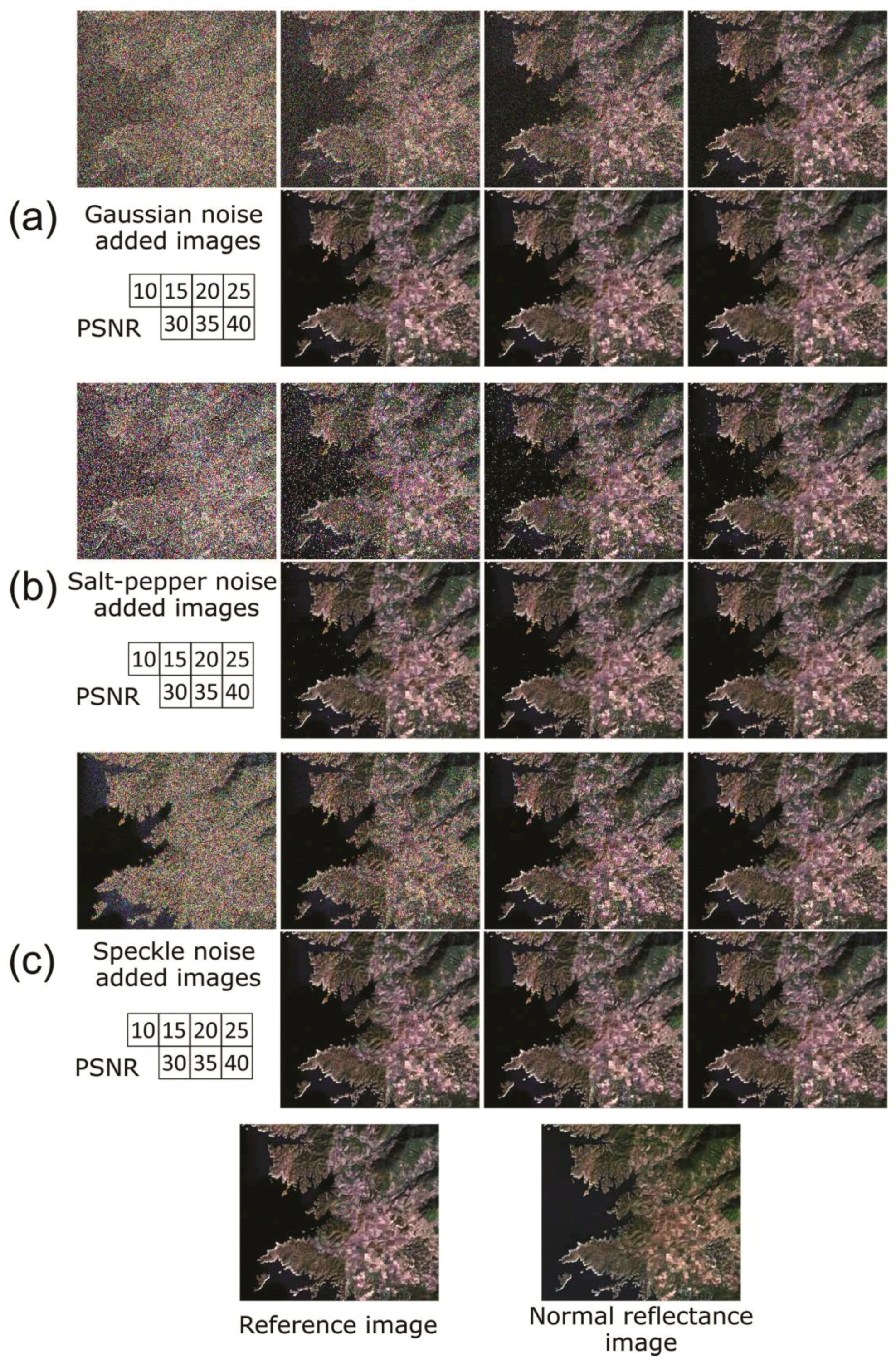
3.1. Image with Added Noise

Each noisy image was constructed by considering the PSNR values. An automatic noise-adding function was used to apply random noise to each satellite image band. In the case of salt–pepper noise, the pixel location may possibly be disturbed by the noise (irrespective of whether it is salt or pepper) more than once, i.e., the first location (row 1, column 1) of the seven-band satellite image data consists of seven pixels, and the noise can either be added or not added to a pixel, some pixels, or all pixels. In the case of additive (zero-mean Gaussian noise) and multiplicative noise (speckle noise), all pixels in each image band were directly afflicted by adding or multiplying by random values. Note that, to produce the intended PSNR, a certain noise parameter is associated with each image band depending on the type of noise. In other words, a noise layer was prepared by using specific parameters such as the variance, mean, and standard deviation, after which the PSNR was calculated from the mean-square error of the original image and the noise layer combined with the original image. This requires the parameters to be assigned a certain value before they are used to target a certain PSNR. The noisy images are shown in Figure 3.

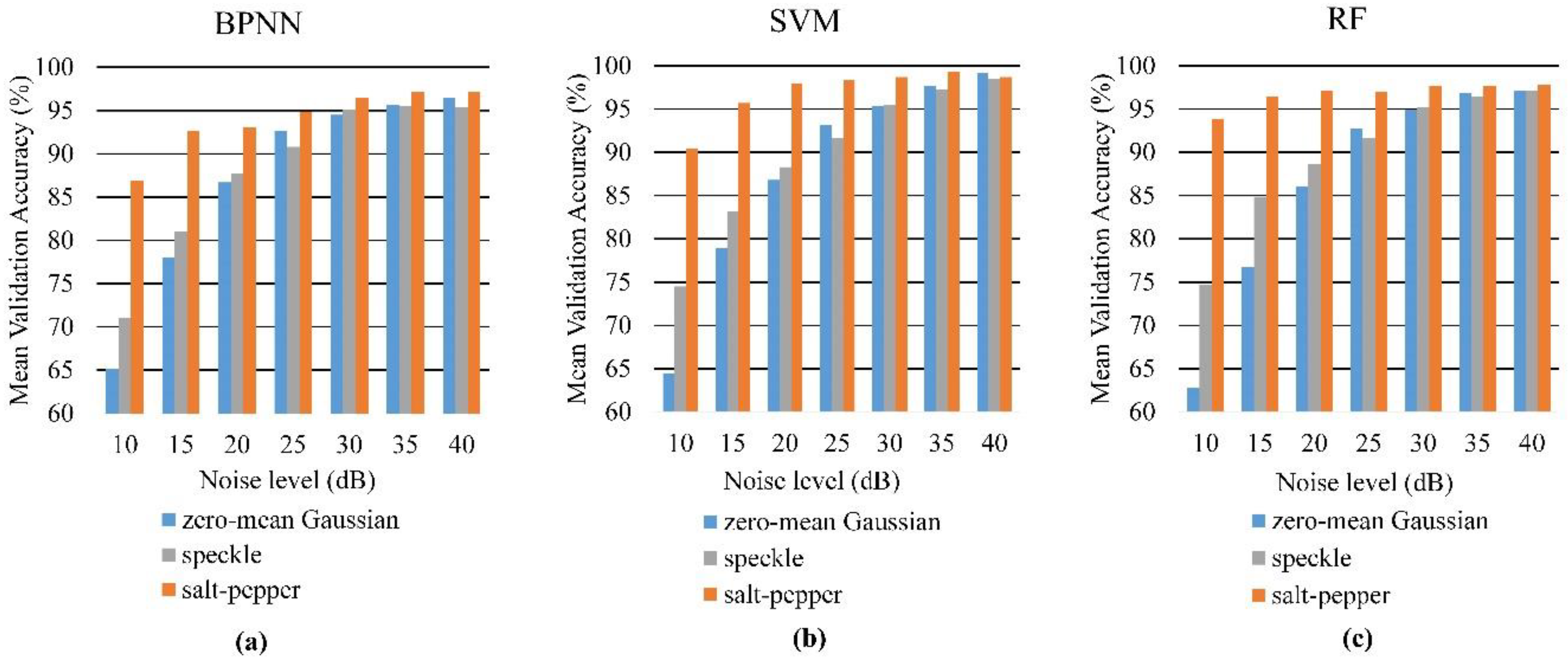
3.2. Classification Results

3.2.1. BPNN

The mean model accuracy (OAm1) and mean validation accuracy (OAV1) obtained by classifying (30 replications) the reference image by the neural network model are 99.1% and 96.7% (K = 0.94). In the case of images without atmospheric correction, the algorithm produced accuracies of 99.0% and 96.4% (K = 0.94) for OAm1 and OAV1, respectively. It is obvious that the value of OAV is fairly low when the algorithm encounters very high noise content. The best validation accuracy (OAV0) of the images to which zero-mean Gaussian noise was added is 65.9% (K = 0.31) at 10 dB, for which the classifier was completely unable to classify the construction class until reaching a PSNR of 30 dB. The accuracy rapidly increased from this percentage to over 90% at 25 dB, then slightly increased to 98.5% (K = 0.97) at 40 dB.
The OAV0 for image classification with added speckle noise at 10 dB is 73.8% (K = 0.52), which differs considerably from the lowest accuracy obtained for the zero-mean Gaussian noise; however, the construction class still cannot be classified until a PSNR of 30 dB is reached. Above 25 dB, the image classification accuracies are higher for images to which zero-mean Gaussian noise was added in comparison to speckle noise. In contrast, the classification accuracies obtained for images with added salt–pepper noise are higher than those to which other types of noise were added, i.e., the mean validation accuracies (OAV1) exceed 85% (K ≥ 0.75) at 10 dB and are over 90% (K ≥ 0.85) for the remaining PSNR levels. The classification accuracies obviously showed that BPNN is affected by all types of noise at increasing noise intensities. Details of the classification accuracies of the BPNN classifiers are presented in Table 3.

3.2.2. SVM

The mean model accuracy (OAm1) and mean validation accuracy (OAV1) obtained from classifying the reference image by the SVM model are as high as the values obtained from non-atmospheric-corrected images, i.e., approximately 99% (K ≥ 0.98). The OAV0 of the images to which zero-mean Gaussian noise was added is 64.5% (K = 0.23) at 10 dB, for which the classifier was completely incapable of classifying the agriculture and construction class until PSNRs of 15 dB and 25 dB, respectively, were reached. In most of the cases, the accuracy increases from this percentage to 99.2% (K = 0.99) at 40 dB. The OAV1 for the classification of images to which speckle noise was added at 10 dB is 74.5% (Kappa = 0.54), which differs by 10% from the value obtained for zero-mean Gaussian noise; however, it is still not possible to classify the construction class until a PSNR of 30 dB is reached. At high noise content (10–20 dB), the classifications of images to which speckle noise was added yielded accuracies higher than those of the datasets afflicted by zero-mean Gaussian noise. Contrary to this, the mean validation accuracies are over 90% (K ≥ 0.83) for all classification tasks that were afflicted by salt–pepper noise. Moreover, the SVM algorithm could model all classes to which this noise was added. Details of the classification accuracies of the SVM classifiers are provided in Table 4.

3.2.3. RF

In the case of RF classifiers, the mean model accuracy (OAm1) and mean validation accuracy (OAV1) obtained by classifying the reference image are 99.1% and 98.8% (K = 0.98), respectively. The algorithm produced the closed OAV1 value for the reference and image without atmospheric correction, which is consistent with the results obtained from the BPNN and SVM. The increasing trends observed for OAm1 and OAV1 for the classification of images to which zero-mean Gaussian and speckle noise was added is similar to that of SVM and BPNN, but the RF classifiers are more effective at high noise intensity. Unexpectedly, the mean validation accuracies reached 93.8% (K ≥ 0.89) for 10 dB salt–pepper noise-afflicted image classifications. Consequently, classifying the construction class, the classification of which is problematic with both BPNN and SVM, remains impossible until PSNRs of 25, 15, and 30 dB are reached with zero-mean Gaussian, salt–pepper, and speckle noise, respectively. Details of the classification accuracies of the RF classifiers are provided in Table 5.

4. Discussion

4.1. Performance of the Classifiers vs. the Reference and the Non-Atmospheric-Corrected Image

The mean kappa coefficients of the same classifier for classification of the reference image and the image without atmospheric correction are very similar. For example, the BPNN produced K = 0.94 for both the classification of reference and non-atmospheric-corrected image, which indicates that there is insignificant difference between the classification result of the images. This proves that the classifications using the three ML classifiers on data from a single date Landsat 8 OLI image may not require absolute atmospheric correction. In other words, the Level 1 Landsat products are already used for land cover classification after digital conversion to reflectance. However, the absolute atmospheric correction is still required in some works, i.e., time-series analysis and multi-sensor image data.

4.2. Analysis of Noise and Classifiers

Zero-mean Gaussian noise, which was used to illustrate that the effect of adding random values to the image pixels has a significant impact on the classification performance of all classifiers in the presence of high-intensity noise, causes the mean validation accuracies to be lower than 66% (K ≤ 0.28) (Figure 4). The three classifiers were unable to classify the construction class unless the noise content was decreased to 25 dB (RF and SVM) and 30 dB (BPNN). Moreover, a noise intensity of 10 dB also caused SVM to fail in the classification of the agriculture class, for which BPNN and RF also produced very low accuracies. These phenomena have their origins in the high variance of noise that was added to the training data. This variance causes additional overlapping of the ranges of values among the categories. Another explanation may be that the addition of noise changed the samples significantly. In other words, increasing the additive or zero-mean Gaussian noise decreases the representativeness of each category by changing the pattern of the samples in some or all of the layers.
We simulated the occurrence of speckle noise on the reference image by multiplying the random values at different PSNRs. It should be noted that, in real situations, speckle noise either exists infrequently or occurs at very low radiance in Landsat 8 OLI data. The effect of speckle noise is quite similar to that of zero-mean Gaussian noise, in that these types of noise decrease the representativeness of the training model of each class. According to the result, the three algorithms can overcome high-intensity speckle noise more effectively than high-intensity zero-mean Gaussian noise. When considering the UA and PA of each class, the commission and omission errors are lower than the classification accuracies for images to which zero-mean Gaussian noise was added. This is attributed to the small change in the product after multiplication of the noise and the low pixel value compared to the original when compared to zero-mean Gaussian images, especially in the case of dark objects such as water bodies and mountain shadows (Figure 3).
Salt and pepper noise is the minimum and maximum of the image pixel values (here they are 0 and 1) and randomly replaces the original pixels. In this case, the replaced noise pixels can be seen as data loss or missing data in the case of salt, and black dots in the case of pepper, which can sometimes be removed from the image by using a mask. However, if the reference data points were located among those pixels removed by the mask, it would be problematic, because it would cause valuable ground truth data points to be lost. In this study, the selected ML algorithms were proved to be robust to this kind of noise. Figure 4 clearly shows the mean validation accuracies (OAV1) of all classifiers higher than 85% (K ≥ 0.76). RF outperforms the other classifiers and has an OAV1 value of 93.8% (K = 0.89) at the highest noise intensity used in this study (10 dB).
The question may arise here as to why salt–pepper noise had a lesser effect than other types of noise in the classification using these classifiers. This can be explained by pointing to the characteristic of the noise. The noise is not applied to all image pixels; instead, it randomly “replaced” the target pixel by certain values. If the set of a training class is not completely replaced by the noise, the remaining unchanged values can be used to represent the pattern of the class. In other words, we have seven layers for training samples, and if only two of these are changed to the same value (even if they are changed to a different value), the remaining five layers, which are strongly representative of the class, are still available for classification. This is a unique characteristic of salt–pepper noise and is different from that of speckle and zero-mean Gaussian noise.
The algorithm used to train the classifiers also plays an important role in the classification. The black box of basic BPNNs returned a final model that consisted of two main parameters: bias and weights. In this sense, the final model truly represents all of the training samples. This is why the BPNN models trained by noisy data provided lower accuracies than others. Normally, we can improve BPNN accuracy by reducing noise in the data or including more representative training samples in the BPNN learning process. SVM separates binary classes using the optimal hyperplane. The final hyperplane is generated by a few support vectors near the boundary area of the two classes. In this investigation of the effect of noise, the SVM is significantly more robust, because of the fact that the SVM’s parameter selection only determines optimal support vectors to construct the final hyperplanes separating each of the categories. This means that the outlier or noise data were confirmed to be mostly excluded from hyperplane construction. Moreover, for the construction class, which has a very small training size disturbed by high noise intensity, SVM seems to be more effective than the other classifiers. In this study, RF outperformed all the classifiers for the classification of images to which salt–pepper noise was added. This is because the RF randomly generated a large number of trees (decision trees) from training data to produce forests, following which the unknown test samples were voted for by all trees in the final step. This means that anomaly values such as noise may not be voted for by the trees.
In a classification using supervised ML algorithms, the representativeness and the number of images used as training data should be of greater concern when the satellite image is afflicted by noise. Considering the training data in Table 1, the reference samples of each class are imbalanced based on the fact that the percentage of each class in the image is not equal. A rough count of the study area, shown in Figure 2, indicates that the water body and forest class accounts for approximately 60% of the image and the remaining 40% consists of pixels in the bare land, agriculture, and construction classes. An examination of the result of the classifications revealed that the construction class always has the lowest accuracies of any of the classifiers. This may come from one or both of the following: (case 1) the construction class contains too few samples to represent the class characteristic in the presence of noise; (case 2) the limitations of remotely sensed data to represent the class for any given pixel resolution. In this study, based on the results, we can strongly assume that the misclassified samples cannot be explained by case 2, because the accuracy result of the reference image classification confirms that the construction class can be properly classified. The classification accuracy of the water body and forest classes was mostly high despite the existence of high noise content, because these classes have sufficient training samples to expose the class characteristic even though it is afflicted by noise.
In our experience, supervised-based classifiers, especially ML classifiers, are sensitive to the structure or pattern of training samples because they learn from these data. For example, two size-fixed agricultural areas of a crop with different planting densities (one is sparse, the other is dense) can generally be seen as different classes in medium-resolution images such as a Landsat image due to the effect of the soil background. The user needs to use this information to train the classifier to produce a reasonable and accurate result. This is similar to the case of noise-afflicted data. If it is not possible to prevent or eliminate noise from data, a more effective approach would be to teach the classifier to understand the noise patterns by increasing the number of training samples or by using training data dispersed across the area.
The experiment in this study was carried out on the assumption that the same variance in noise occurred in every layer, whereas the occurrence of real noise varies as it is only found in some bands or as a mixture of different types and intensities of noise. We elucidated the gap by expressing the simulated noise by PSNR as an appropriate way in which the real noise can also be measured by this measurement. However, the intensity of real noise is normally not as high as the noise levels we investigated. The experimental design aimed to determine the effect of noise and to test the performance of the ML algorithms. Consequently, the wide range of noise levels was used to capture the behavior and effects of noise.

4.3. Advanced Extension of the MLs

Recent decades have seen various extensions of the BPNN (e.g., [54,55,56]), SVM (e.g., [56,57]), and RF (e.g., [56,58]) algorithms that were developed to overcome their drawbacks and, we believe, can perform more effectively than the basic versions of these algorithms. We suggest that readers who require a very high accuracy use the extended version or a noise filter [59,60,61]. In general, the application of advanced MLs depends greatly on the related theory or technique. For example, fuzzy set concepts [62] are usually attached to basic MLs to make the decision space in categorizing more flexible (fuzzy random forest [63]; fuzzy nonlinear proximal SVM [64]; fuzzy-NN [65]). Markov-systems-based techniques also belong to the leading trend of increasing the classification accuracy (Markov-random-field-based SVM [57]; MLP-Markov chain models [66]). Beside the abovementioned extensions, there are various combinable algorithms that exist in classification field, such as a particle filter [35] and genetic algorithm.
Although the robustness of the basic BPNN towards noises observed in this study was lower than that of RF and SVM, the new-generation neural networks, especially deep learning, are outstanding among other advanced learning algorithms [67]. Deep learning algorithms automatically extract features and abstractions from the underlying data. Numerous reports in the literature have demonstrated that data representations obtained from a deep learning model often yield better results, e.g., improved classification modeling. For example, Hu and Yi (2016) obtained a reasonable result for ground point extraction (for digital terrain modeling) by employing deep convolution neural networks using 17 million labeled Airborne laser scanning (ALS) points [55]. Moreover, Chen et al. (2014) developed a hybrid framework of principle component analysis (PCA), deep learning architecture, and logistic regression for accurate hyperspectral data classification that yielded higher accuracy than RBF-SVM [68]. The examples demonstrated the performance of deep learning over complicated works when a large number of training samples are available.
Nevertheless, the majority of users still use the original algorithms without any complicated extensions. Our work is not only intended to assist private users with the selection of appropriate classifiers for their work, but also to transfer an understanding of remote sensing data to algorithm developers. Future work on other ML classifiers, especially on new algorithms invented in the last decade, would be necessary to compare them to the existing algorithms.

5. Conclusions

In this study, we investigated the effects of adding simulated zero-mean Gaussian, salt–pepper, and speckle noise on image classification performance. Three well-known machine-learning classifiers, i.e., back-propagation neural network (BPNN), support vector machine (SVM), and random forest (RF), with the most basic parameter settings, were used for the classifications. A Landsat 8 OLI scene of Srinakarin dam, Kanchanaburi Province, Thailand, acquired under cloud-free conditions with absolute atmospheric correction, was used as reference data for noise affliction. We specified the same number of usable training data for all classifiers. The experiment started by classifying the reference image by the classifiers, after which the results were set as the baseline accuracy for interpretation. The reference image was then contaminated by different levels of noise at peak signal-to-noise ratios (PSNRs) ranging from 10 to 40 dB (in increments of 5 dB). Finally, 21 noisy images were obtained and separately classified by the classifiers. As expected, the lower the PSNR (high noise intensity), the lower the accuracy. All classifiers provided accuracies over 96% for the reference and the image without atmospheric correction. This means that absolute atmospheric correction in single date classification is unnecessary for images acquired under clear weather conditions. We suggest from our experiment that an increase in the number of training and collecting samples dispersed in various patterns across the study area facilitates the improvement of the representativeness of the class when the data is afflicted by high-intensity noise. More specifically, in terms of the performance of the classifiers, the BPNN models provided accuracies lower than others in very high noise intensity, because the algorithm strongly depends on the values of the training samples. According to the results, SVM often provides a high accuracy because SVM parameter selection can be used to ensure that only optimal support vectors are found to construct the final hyperplanes separating each of the categories, and the minor fluctuations caused by noise were confirmed to mostly be excluded from model construction. RF outperformed all of the classifiers in salt–pepper noise added image classifications. However, although in this study the three ML classifiers proved to be very robust to low-to-medium noise intensity (PSNR > 20) without using any filter or extension, we suggest taking advantage of a noise filter or the advanced extensions of these ML classifiers, especially for cases requiring very high accuracy (almost 100%).

Author Contributions

Conceptualization, S.B.; methodology, S.B.; software, S.B. and B.K.A.; validation, S.B. and W.C.; formal analysis, S.B.; investigation, C.C.; resources, C.C. and M.X.; data Curation, S.B. and W.C.; writing—original draft preparation, S.B.; writing—review and editing, S.B.; visualization, S.B. and B.K.A.; supervision, C.C. and W.C.; project administration, C.C., M.X., and X.N.; funding acquisition, C.C.

Funding

This research was financed by the Natural Science Foundation of China (No. 41601368), the National Key Research and Development Program of China (No. 2016YFB0501505), and the Instrument Development Project of the State Key Laboratory of Remote Sensing Science (No. Y7Y01100KZ).

Acknowledgments

The authors would like to extend their gratitude to the Geo-Informatics and Space Technology Development Agency (GISTDA), Thailand, for the reference data, and to Peerapong Torteeka for his assistance in revising the algorithms. Sornkitja Boonprong would like to express his gratitude to the Royal Thai Government for their support and the scholarship provided. The authors would also like to thank the anonymous reviewers for their insightful comments, which have significantly improved this paper.

Conflicts of Interest

The authors declare no conflict of interest.

References

  1. Song, M.; Civco, D.L.; Hurd, J.D. A competitive pixel-object approach for land cover classification. Int. J. Remote Sens. 2005, 26, 4981–4997. [Google Scholar] [CrossRef]
  2. Petrou, Z.I.; Kosmidou, V.; Manakos, I.; Stathaki, T.; Adamo, M.; Tarantino, C.; Tomaselli, V.; Blonda, P.; Petrou, M. A rule-based classification methodology to handle uncertainty in habitat mapping employing evidential reasoning and fuzzy logic. Pattern Recognit. Lett. 2014, 48, 24–33. [Google Scholar] [CrossRef]
  3. Simonetti, E.; Simonetti, D.; Preatoni, D. Phenology-Based Land Cover Classification Using Landsat 8 Time Series; European Commission Joint Research Center: Ispra, Italy, 2014. [Google Scholar]
  4. Loosvelt, L.; Peters, J.; Skriver, H.; Lievens, H.; Van Coillie, F.M.B.; De Baets, B.; Verhoest, N.E.C. Random Forests as a tool for estimating uncertainty at pixel-level in SAR image classification. Int. J. Appl. Earth Obs. 2012, 19, 173–184. [Google Scholar] [CrossRef]
  5. Al-amri, S.; Kalyankar, N.; Khamitkar, S. A Comparative Study of Removal Noise from Remote Sensing Image. IJCSI Int. J. Comput. Sci. 2010, 7, 32–36. [Google Scholar]
  6. Dierking, W.; Dall, J. Sea Ice Deformation State from Synthetic Aperture Radar Imagery—Part II: Effects of Spatial Resolution and Noise Level. IEEE Trans. Geosci. Remote Sens. 2008, 46, 2197–2207. [Google Scholar] [CrossRef]
  7. Barber, M.; Grings, F.; Perna, P.; Piscitelli, M.; Maas, M.; Bruscantini, C.; Jacobo-Berlles, J.; Karszenbaum, H. Speckle Noise and Soil Heterogeneities as Error Sources in a Bayesian Soil Moisture Retrieval Scheme for SAR Data. IEEE J. Sel. Top. Appl. Earth Obs. Remote Sens. 2012, 5, 942–951. [Google Scholar] [CrossRef]
  8. Benz, U.; Hofmann, P.; Willhauck, G.; Lingenfelder, I.; Heynen, M. Multi-resolution, object-oriented fuzzy analysis of remote sensing data for GIS-ready information. ISPRS J. Photogramm. Remote Sens. 2004, 58, 239–258. [Google Scholar] [CrossRef] [Green Version]
  9. Celik, T.; Ma, K.K. Unsupervised Change Detection for Satellite Images Using Dual-Tree Complex Wavelet Transform. IEEE Trans. Geosci. Remote Sens. 2010, 48, 1199–1210. [Google Scholar] [CrossRef]
  10. Mohammed, K.; Mohamed, D.; Philippe, C. Magnitude-phase of the dual-tree quaternionic wavelet transform for multispectral satellite image denoising. EURASIP J. Image Video Process. 2014, 2014, 1–16. [Google Scholar]
  11. Vijay, M.; Devi, L.S. Speckle Noise Reduction in Satellite Images Using Spatially Adaptive Wavelet Thresholding. Int. J. Comput. Sci. Inf. Technol. 2012, 3, 3432–3435. [Google Scholar]
  12. Bhosale, N.P.; Manza, R.R. Analysis of Effect of Noise Removal Filters on Noisy Remote Sensing Images. Int. J. Sci. Eng. Res. 2013, 4, 1151. [Google Scholar]
  13. Data Loss, Landsat Missions, USGS. Available online: https://landsat.usgs.gov/data-loss (accessed on 5 June 2018).
  14. Charoenjit, K.; Zuddas, P.; Allemand, P.; Pattanakiat, S.; Pachana, K. Estimation of biomass and carbon stock in Para rubber plantations using object-based classification from Thaichote satellite data in Eastern Thailand. J. Appl. Remote Sens. 2015, 9, 096072. [Google Scholar] [CrossRef] [Green Version]
  15. Yahya, N.; Kamel, N.S.; Malik, A.S. Subspace-Based Technique for Speckle Noise Reduction in SAR Images. IEEE Trans. Geosci. Remote Sens. 2014, 52, 6257–6271. [Google Scholar] [CrossRef]
  16. Raney, R.K. Radar Fundamentals: Technical Perspective. In Principles and Applications of Imaging Radar, Manual of Remote Sensing, 3rd ed.; John Wiley and Sons Inc.: Toronto, ON, Canada, 1998; Chapter 2. [Google Scholar]
  17. Mansourpour, M.; Rajabi, M.A.; Blais, J.A.R. Effects and Performance of Speckle Noise Reduction Filters on Active Radar and SAR Images. Proc. ISPRS 2006, 36, W41. [Google Scholar]
  18. Nobrega, R.A.A.; Quintanilha, J.A.; O’Hara, C.G. A noise-removal approach for LIDAR intensity images using anisotropic diffusion filtering to preserve object shape characteristics. In Proceedings of the ASPRS 2007 Annual Conference, Tampa, FL, USA, 7–11 May 2007. [Google Scholar]
  19. Mulder, V.L.; de Bruin, S.; Schaepman, M.E.; Mayr, T.R. The use of remote sensing in soil and terrain mapping—A review. Geoderma 2011, 162, 1–19. [Google Scholar] [CrossRef]
  20. Zhu, X.; Wu, X. Class Noise vs. Attribute Noise: A Quantitative Study of Their Impacts. Artif. Intell. Rev. 2004, 22, 177–210. [Google Scholar] [CrossRef]
  21. Breiman, L. Random Forests. Mach. Learn. 2001, 45, 5–32. [Google Scholar] [CrossRef] [Green Version]
  22. Alsmadi, M.K.S.; Omar, K.B.; Noah, S.A. Back Propagation Algorithm: The Best Algorithm among the Multi-layer Perceptron Algorithm. Int. J. Comput. Sci. Netw. Secur. 2009, 9, 378–383. [Google Scholar]
  23. Caruana, R.; Niculescu-Mizil, A. An Empirical Comparison of Supervised Learning Algorithms. In Proceedings of the 23rd International Conference on Machine Learning, Pittsburgh, PA, USA, 25–29 June 2006; pp. 161–168. [Google Scholar]
  24. Dey, A. Machine Learning Algorithms: A. Review. Int. J. Comput. Sci. Inf. Technol. 2016, 7, 1174–1179. [Google Scholar]
  25. Kotsiantis, S.B. Supervised Machine Learning: A Review of Classification Techniques. Informatica 2007, 31, 249–268. [Google Scholar]
  26. Singh, A.; Thakur, N.; Sharma, A. A review of supervised machine learning algorithms. In Proceedings of the 2016 3rd International Conference on Computing for Sustainable Global Development (INDIACom), New Delhi, India, 16–18 March 2016; pp. 1310–1315. [Google Scholar]
  27. Crisci, C.; Ghattas, B.; Perera, G. A review of supervised machine learning algorithms and their applications to ecological data. Ecol. Model. 2012, 240, 113–122. [Google Scholar] [CrossRef]
  28. Lorena, A.C.; Jacintho, L.F.O.; Siqueira, M.F.; Giovanni, R.D.; Lohmann, L.G.; de Carvalho, A.C.P.L.F.; Yamamoto, M. Comparing machine learning classifiers in potential distribution modelling. Expert Syst. Appl. 2011, 38, 5268–5275. [Google Scholar] [CrossRef]
  29. Mariana, B.; Lucian, D. Random forest in remote sensing: A review of application and future directions. ISPRS J. Photogramm. Remote Sens. 2016, 114, 24–31. [Google Scholar]
  30. Rodriguez-Galiano, V.F.; Ghimire, B.; Rogan, J.; Chica-Olmo, M.; Rigol-Sanchez, J.P. An assessment of the effectiveness of a random forest classifier for land-cover classification. ISPRS J. Photogramm. Remote Sens. 2012, 67, 93–104. [Google Scholar] [CrossRef]
  31. Loosvelt, L.; Peters, J.; Skriver, H.; De Baets, B.; Verhoest, N.E.C. Impact of Reducing Polarimetric SAR Input on the Uncertainty of Crop Classifications Based on the Random Forests Algorithm. IEEE Trans. Geosci. Remote Sens. 2012, 50, 4185–4200. [Google Scholar] [CrossRef]
  32. Freund, Y.; Schapire, R.E. Experiments with a new boosting algorithm. In Proceedings of the Thirteenth International Conference on International Conference on Machine Learning, Bari, Italy, 3–6 July 1996; pp. 148–156. [Google Scholar]
  33. Mountrakis, G.; Im, J.; Ogole, C. Support vector machines in remote sensing: A review. ISPRS J. Photogramm. Remote Sens. 2011, 66, 247–259. [Google Scholar] [CrossRef]
  34. Insom, P.; Cao, C.; Boonsrimuang, P.; Liu, D.; Saokarn, A.; Yomwan, P.; Xu, Y. A Support Vector Machine-Based Particle Filter Method for Improved Flooding Classification. IEEE Geosci. Remote Sens. Lett. 2015, 12, 1943–1947. [Google Scholar] [CrossRef]
  35. Foody, G.M.; Mathur, A. Toward intelligent training of supervised image classifications: Directing training data acquisition for SVM classification. Remote Sens. Environ. 2004, 93, 107–117. [Google Scholar] [CrossRef]
  36. Dalponte, M.; Bruzzone, L.; Gianelle, D. Fusion of Hyperspectral and LIDAR Remote Sensing Data for Classification of Complex Forest Areas. IEEE Trans. Geosci. Remote Sens. 2008, 46, 1416–1427. [Google Scholar] [CrossRef] [Green Version]
  37. Senf, C.; Leitao, P.J.; Pflugmacher, D.; Linden, S.V.D.; Hostert, P. Mapping land cover in complex Mediterranean landscapes using Landsat: Improved classification accuracies fromintegrating multi-seasonal and synthetic imagery. Remote Sens. Environ. 2015, 156, 527–536. [Google Scholar] [CrossRef]
  38. Pal, M.; Foody, G.M. Feature Selection for Classification of Hyperspectral Data by SVM. IEEE Trans. Geosci. Remote Sens. 2010, 48, 2297–2307. [Google Scholar] [CrossRef] [Green Version]
  39. Cherkassky, V.; Ma, Y. Practical selection of SVM parameters and noise estimation for SVM regression. Neural Netw. 2004, 17, 113–126. [Google Scholar] [CrossRef] [Green Version]
  40. Tseng, M.H.; Chen, S.J.; Hwang, G.H.; Shen, M.Y. A genetic algorithm rule-based approach for land-cover classification. ISPRS J. Photogramm. Remote Sens. 2008, 63, 202–212. [Google Scholar] [CrossRef]
  41. Suliman, A.; Zhang, Y. A Review on Back-Propagation Neural Networks in the Application of Remote Sensing Image Classification. J. Earth Sci. Eng. 2015, 5, 52–65. [Google Scholar]
  42. Paola, J.D.; Schowengerdt, R.A. A review and analysis of backpropagation neural networks for classification of remotely-sensed multi-spectral imagery. Int. J. Remote Sens. 2007, 16, 3033–3058. [Google Scholar] [CrossRef]
  43. Burzzone, L.; Fernandez, P.D.; Cossu, R. An incremental learning classifier for remote-sensing images. In Proceedings of the IEEE 1999 International Geoscience and Remote Sensing Symposium, Hamburg, Germany, 28 June–2 July 1999; pp. 2483–2485. [Google Scholar]
  44. Avanaki, M.R.N.; Laissue, P.; Podoleanu, A.; Hojjat, S.A. Denoising based on noise parameter estimation in speckled OCT images using neural network. In Proceedings of the 1st Canterbury Workshop and School in Optical Coherence Tomography and Adaptive Optics, Canterbury, UK, 30 December 2008. [Google Scholar] [CrossRef]
  45. Kofidis, E.; Theodoridis, S.; Kotropoulos, C.; Pitas, I. Application of Neural Networks and Order Statistics Filters to Speckle Noise Reduction in Remote Sensing Imaging. In Neurocomputation in Remote Sensing Data Analysis; Springer: Berlin/Heidelberg, Germany, 1997. [Google Scholar] [CrossRef]
  46. Silva, I.B.V.D.; Adeodato, P.J.L. PCA and Gaussian noise in MLP neural network training improve generalization in problems with small and unbalanced data sets. In Proceedings of the 2011 International Joint Conference on Neural Networks, San Jose, CA, USA, 31 July–5 August 2011; pp. 2664–2669. [Google Scholar] [CrossRef]
  47. Corner, B.R.; Narayanan, R.M.; Reichenbach, S.E. Noise estimation in remote sensing imagery using data masking. Int. J. Remote Sens. 2003, 24, 689–702. [Google Scholar] [CrossRef]
  48. Breiman, L. Manual on Setting Up, Using, and Understanding Random Forests v3.1; Department of Statistics, University of California: Berkeley, CA, USA, 2002. [Google Scholar]
  49. Moller, M.F. A scaled conjugate gradient algorithm for fast supervised learning. Neural Netw. 1993, 6, 525–533. [Google Scholar] [CrossRef]
  50. Boser, B.E.; Guyon, I.M.; Vapnik, V.N. A training algorithm for optimal margin classifiers. In Proceedings of the Fifth Annual Workshop on Computational Learning Theory, Pittsburgh, PA, USA, 27–29 July 1992; pp. 144–152. [Google Scholar]
  51. Cortes, C.; Vapnik, V. Support-vector networks. Mach. Learn. 1995, 20, 273–297. [Google Scholar] [CrossRef] [Green Version]
  52. Liaw, A.; Wiener, M. Classification and Regression by Random Forest. R News 2002, 2, 18–22. [Google Scholar]
  53. Chang, C.C.; Lin, C.J. LIBSVM: A library for support vector machine. ACM Trans. Intell. Syst. Technol. 2011, 2, 27. [Google Scholar] [CrossRef]
  54. Rodríguez-Fernández, N.J.; Kerr, Y.H.; van der Schalie, R.; Al-Yaari, A.; Wigneron, J.P.; de Jeu, R.; Richaume, P.; Dutra, E.; Mialon, A.; Drusch, M. Long Term Global Surface Soil Moisture Fields Using an SMOS-Trained Neural Network Applied to AMSR-E Data. Remote Sens. 2016, 8, 959. [Google Scholar] [CrossRef]
  55. Hu, X.; Yuan, Y. Deep-Learning-Based Classification for DTM Extraction from ALS Point Cloud. Remote Sens. 2016, 8, 730. [Google Scholar] [CrossRef]
  56. Li, X.; Chen, W.; Cheng, X.; Wang, L. A Comparison of Machine Learning Algorithms for Mapping of Complex Surface-Mined and Agricultural Landscapes Using ZiYuan-3 Stereo Satellite Imagery. Remote Sens. 2016, 8, 514. [Google Scholar] [CrossRef]
  57. Yu, H.; Gao, L.; Li, J.; Li, S.S.; Zhang, B.; Benediktsson, J. Spectral-Spatial Hyperspectral Image Classification Using Subspace-Based Support Vector Machines and Adaptive Markov Random Fields. Remote Sens. 2016, 8, 355. [Google Scholar] [CrossRef]
  58. Wessels, K.J.; van den Bergh, F.; Roy, D.P.; Salmon, B.P.; Steenkamp, K.C.; MacAlister, B.; Swanepoel, D.; Jewitt, D. Rapid Land Cover Map Updates Using Change Detection and Robust Random Forest Classifiers. Remote Sens. 2016, 8, 888. [Google Scholar] [CrossRef]
  59. Shrestha, R.; Wynne, R.H. Estimating biophysical parameters of individual trees in an urban environment using small footprint discrete-return imaging Lidar. Remote Sens. 2012, 4, 484–508. [Google Scholar] [CrossRef]
  60. Boonprong, S.; Cao, C.; Torteeka, P.; Chen, W. A Novel Classification Technique of Landsat-8 OLI Image-Based Data Visualization: The Application of Andrews’ Plots and Fuzzy Evidential Reasoning. Remote Sens. 2017, 9, 427. [Google Scholar] [CrossRef]
  61. Chang, E.S.; Hung, C.C.; Liu, W.; Yin, J. A Denoising Algorithm for Remote Sensing Images with Impulse Noise. In Proceedings of the IEEE International Geoscience and Remote Sensing Symposium (IGARSS), Beijing, China, 10–15 July 2016; pp. 2905–2908. [Google Scholar]
  62. Zadeh, L.A. Fuzzy Sets. Inf. Control 1965, 8, 338–355. [Google Scholar] [CrossRef]
  63. Bonissone, P.; Cadenas, J.M.; Garrido, M.C.; Díaz-Valladares, R.A. A fuzzy random forest. Int. J. Approx. Reason. 2010, 51, 729–747. [Google Scholar] [CrossRef]
  64. Zhong, X.; Li, J.; Dou, H.; Deng, S.; Wang, G.; Jiang, Y.; Wang, Y.; Zhou, Z.; Wang, L.; Yan, F. Fuzzy Nonlinear Proximal Support Vector Machine for Land Extraction Based on Remote Sensing Image. PLoS ONE 2013, 8, e69434. [Google Scholar] [CrossRef] [PubMed]
  65. Goodarzi, R.; Mokhtarzade, M.; Zoej, M.J.V. A Robust Fuzzy Neural Network Model for Soil Lead Estimation from Spectral Features. Remote Sens. 2015, 7, 8416–8435. [Google Scholar] [CrossRef] [Green Version]
  66. Ozturk, D. Urban Growth Simulation of Atakum (Samsun, Turkey) Using Cellular Automata-Markov Chain and Multi-Layer Perceptron-Markov Chain Models. Remote Sens. 2015, 7, 5918–5950. [Google Scholar] [CrossRef] [Green Version]
  67. Najafabadi, M.M.; Villanustre, F.; Khoshgoftaar, T.M.; Seliya, N.; Wald, R.; Muharemagic, E. Deep learning applications and challenges in big data analytics. J. Big Data 2015, 2, 1–21. [Google Scholar] [CrossRef]
  68. Chen, Y.; Lin, Z.; Zhao, X.; Wang, G.; Gu, Y. Deep Learning-Based Classification of Hyperspectral Data. IEEE J. Sel. Top. Appl. Earth Obs. Remote Sens. 2014, 7, 2094–2107. [Google Scholar] [CrossRef]
Figure 1. Experimental flow.
Ijgi 07 00274 g001
Figure 2. True color image of the study area.
Ijgi 07 00274 g002
Figure 3. Twenty-three satellite images with added noise in different peak signal-to-noise ratios (PSNRs): (a) Gaussian noise, (b) salt–pepper noise, and (c) speckle noise (true color image; R = band 4, G = band 3, and B = band 2).
Ijgi 07 00274 g003
Figure 4. Mean validation accuracy trends of (a) neural network, (b) support vector machine, and (c) random forest classifier in relation to different noise levels and types.
Ijgi 07 00274 g004
Table 1. Number of samples of modeling and application testing datasets.
ClassesDescriptionsM *A *
AgricultureArtificial planting area/no harvested area included504126
Bare landLand used without vegetation cover440110
ConstructionHouses, roads, and any man-made construction8020
Water bodyWater bodies such as ponds, lakes, and rivers34486
ForestArea covered by natural and unused vegetation, mountain shadow2048512
Total3416854
* Modeling data (M) and application testing (A) data.
Table 2. Parameter tuning of all classifiers.
ClassifiersCross-Validation Approaches/Parameters
Random forests (RF)ntree = {500, 1000, 1500, 2000}, mtry = {2, 3, 4, 5}, 30 replications
Support vector machines (SVM)Grid-search cross-validation approach, radial basis function kernel, 30 replications
Back-propagation neural networks (BPNN)Scale conjugated gradient optimization, 70% training, 15% testing, 15% validating, hidden nodes = {5, 10, 15, 20, 40, 60}, 30 replications
The optimized models are different for each observed image.
Table 3. Classification accuracies of the BPNN classifiers.
RINIG10G15G20G25G30G35G40SP10SP15SP20SP25SP30SP35SP40SPK10SPK15SPK20SPK25SPK30SPK35SPK40
PA199.297.67.138.169.887.392.191.396.078.694.490.595.296.898.496.827.846.872.284.994.491.393.7
PA297.399.146.481.886.495.597.397.398.290.996.497.397.398.299.110044.576.490.095.597.397.399.1
PA395.085.000005.070.085.000075.080.095.095.0000030.065.080.0
PA410010039.576.791.910010010010081.491.910097.710010010087.2100100100100100100
PA599.899.691.691.894.396.998.099.099.497.797.597.397.999.699.499.692.093.994.396.397.798.899.8
UA198.499.247.454.571.585.389.998.398.488.488.892.792.398.499.210040.756.773.482.389.595.099.2
UA298.295.657.381.187.290.591.593.994.784.792.290.794.796.498.298.253.875.084.687.593.993.097.3
UA395.0100000050.087.510000083.388.990.590.5000075.092.994.1
UA410010060.777.694.096.610010010094.698.894.510010010010087.293.5100100100100100
UA599.899.468.082.589.895.496.597.399.091.295.095.698.499.299.699.479.788.191.795.297.597.798.3
OAm099.799.990.693.796.497.998.699.699.798.298.698.599.499.699.899.893.996.296.897.698.899.399.7
OAV099.398.965.978.987.293.395.197.198.590.094.094.396.898.699.299.273.883.188.992.695.896.898.4
K00.990.980.310.620.780.890.920.950.970.830.900.900.950.980.990.990.520.700.810.870.930.950.97
OAm199.199.090.393.496.297.798.498.999.096.898.198.298.898.999.199.392.995.396.497.398.498.898.8
OAV196.796.465.278.086.792.794.595.796.586.992.693.194.996.597.197.271.181.087.790.895.195.595.4
K10.940.940.280.600.770.880.900.930.940.760.870.880.910.940.950.950.460.660.790.840.920.920.92
OAm20.600.952.510.330.190.340.280.410.340.280.150.150.110.100.290.281.341.170.620.790.140.200.93
OAV22.143.450.550.450.300.300.250.600.765.320.680.481.110.771.171.143.303.262.062.770.380.483.40
K20.0600.0390.0170.0080.0050.0050.0050.0110.0130.1430.0120.0080.0190.0130.0200.0200.0900.0720.0420.0520.0070.0090.061
RI = reference image; NI = non-atmospheric-corrected image; G(i) = zero-mean Gaussian noise; SP(i) = salt–pepper noise; SPK(i) = speckle noise; OAm(r) = self-model accuracy; OAV(r) = validation accuracy; K(r) = Cohen’s kappa; UA(x) = user’s accuracy; PA(x) = production accuracy; x (class) = {1 = agriculture, 2 = bare land, 3 = construction, 4 = water body, 5 = forest}; i = peak signal-to-noise ratio (dB); r = {0 = best, 1 = mean, 2 = standard deviation}.
Table 4. Classification accuracies of the SVM classifiers.
RINIG10G15G20G25G30G35G40SP10SP15SP20SP25SP30SP35SP40SPK10SPK15SPK20SPK25SPK30SPK35SPK40
PA199.297.6026.268.388.990.594.497.677.090.595.296.897.698.496.025.449.267.582.591.391.394.4
PA210098.237.384.587.392.797.310010090.997.398.299.196.499.198.252.773.689.190.998.298.299.1
PA31009500010.040.055.090.010.065.085.085.090.095.095.0000040.080.085.0
PA410010027.976.794.298.810010010087.297.710010010010010089.598.8100100100100100
PA599.699.694.994.393.496.798.099.299.697.597.999.099.499.699.699.492.094.394.996.397.799.099.6
UA110098.4062.368.383.691.998.399.285.894.296.098.498.499.298.447.859.070.880.689.895.099.2
UA298.298.255.484.588.190.393.994.897.390.993.097.398.297.298.298.257.479.484.587.793.194.796.5
UA310010000066.788.910010025.081.310094.494.795.086.4000088.9100100
UA410010068.675.992.097.710010010096.297.710010010010010084.695.5100100100100100
UA599.899.265.280.090.095.796.497.799.491.697.198.498.899.099.699.279.287.091.494.197.198.198.5
OAm099.599.464.577.287.293.398.798.198.889.496.298.198.398.799.099.275.985.088.192.596.197.998.8
OAV099.699.164.579.086.893.295.797.799.290.595.998.198.798.799.398.774.783.388.491.795.797.498.5
K00.990.980.230.610.770.880.930.960.990.830.930.970.980.980.990.980.540.700.800.860.930.960.97
OAm199.599.464.577.287.293.398.798.198.889.496.298.198.398.799.099.275.985.088.192.596.197.998.8
OAV199.699.164.579.086.893.295.497.799.290.495.798.098.498.799.398.774.583.288.391.695.597.398.5
K10.990.980.230.610.770.880.920.960.990.830.930.970.970.980.990.980.530.700.800.860.920.950.97
OAm20.000.000.000.000.000.000.000.000.000.000.000.000.000.000.000.000.000.000.000.000.000.000.00
OAV20.020.000.000.040.000.000.060.000.000.060.140.050.120.000.040.000.080.040.060.060.040.070.04
K20.0000.0000.0000.0010.0000.0000.0010.0000.0000.0010.0020.0010.0020.0000.0010.0000.0020.0010.0010.0010.0010.0010.001
Table 5. Classification accuracies of the RF classifiers.
RINIG10G15G20G25G30G35G40SP10SP15SP20SP25SP30SP35SP40SPK10SPK15SPK20SPK25SPK30SPK35SPK40
PA197.695.210.323.866.784.992.996.094.487.393.794.494.494.495.295.227.857.971.483.392.993.795.2
PA210010045.581.890.096.497.398.298.295.599.198.299.110099.110050.980.092.793.699.198.297.3
PA39570.000010.020.045.065.0035.060.060.060.070.070.0000025.055.065.0
PA410010031.469.890.798.810098.810098.898.810010010010010088.498.8100100100100100
PA599.499.488.993.493.996.997.999.299.498.899.299.099.099.699.699.493.294.394.796.597.798.899.2
UA110099.235.146.271.884.390.797.697.590.997.597.596.799.299.299.241.760.872.682.090.095.296.0
UA296.594.853.278.385.392.292.295.693.992.192.493.994.893.294.895.757.180.784.388.092.493.994.7
UA310010000066.710081.892.9010092.385.710093.393.3000010091.7100
UA410010050.982.294.097.710010010098.810098.910010010010091.697.7100100100100100
UA599.498.567.979.589.495.096.597.598.594.997.198.198.398.598.698.581.089.892.794.597.197.998.3
OAm099.798.967.078.089.593.996.398.098.595.397.998.798.898.999.098.978.087.988.993.696.398.098.8
OAV099.298.263.877.886.993.295.497.397.894.496.897.497.598.098.298.275.485.489.392.395.797.197.7
K00.990.970.280.580.770.880.920.950.960.900.950.960.960.970.970.970.550.750.820.870.930.950.96
OAm199.198.563.376.686.892.695.497.397.994.597.097.697.998.398.398.376.785.688.392.595.397.197.9
OAV198.897.862.876.786.092.794.996.997.193.896.497.197.097.797.797.874.784.888.791.695.296.597.1
K10.980.960.250.570.750.870.910.950.950.890.940.950.950.960.960.960.540.740.810.860.920.940.95
OAm20.270.251.351.050.910.710.600.410.490.580.470.470.440.330.370.350.790.920.500.620.530.510.46
OAV20.190.170.810.530.470.310.280.250.300.280.220.200.290.250.270.250.460.420.300.310.270.270.25
K20.0030.0030.0160.0110.0090.0050.0050.0040.0050.0050.0040.0030.0050.0040.0050.0040.0090.0070.0050.0050.0050.0050.004

