Article

Semi-Supervised Classification for Hyperspectral Images Based on Multiple Classifiers and Relaxation Strategy

1
College of Urban and Environment, Liaoning Normal University, Dalian 116029, China
2
College of Computer Science, Liaoning Normal University, Dalian 116081, China
*
Author to whom correspondence should be addressed.
ISPRS Int. J. Geo-Inf. 2018, 7(7), 284; https://doi.org/10.3390/ijgi7070284
Submission received: 11 May 2018 / Revised: 11 July 2018 / Accepted: 19 July 2018 / Published: 23 July 2018

Abstract

:
Hyperspectral image (HSI) classification is a fundamental and challenging problem in remote sensing and its various applications. However, it is difficult to perfectly classify remotely sensed hyperspectral data by directly using classification techniques developed in pattern recognition. This is partially owing to a multitude of noise points and the limited training samples. Based on multinomial logistic regression (MLR), the local mean-based pseudo nearest neighbor (LMPNN) rule, and the discontinuity preserving relaxation (DPR) method, in this paper, a semi-supervised method for HSI classification is proposed. In pre-processing and post-processing, the DPR strategy is adopted to denoise the original hyperspectral data and improve the classification accuracy, respectively. The application of two classifiers, MLR and LMPNN, can automatically acquire more labeled samples in terms of a few labeled instances per class. This is termed the pre-classification procedure. The final classification result of the HSI is obtained by employing the MLRsub approach. The effectiveness of the proposal is experimentally evaluated by two real hyperspectral datasets, which are widely used to test the performance of the HSI classification algorithm. The comparison results using several competing methods confirm that the proposed method is effective, even for limited training samples.

1. Introduction

Owing to the special advantages of a wide spectral range, high spectral resolution, and continuous spectral curve, hyperspectral remote-sensing images have been widely applied in earth observation [1,2]. As a fundamental and challenging problem in remote sensing, hyperspectral image (HSI) classification and its various applications have attracted increasing attention in recent years. Many methods have been introduced to classify HSI, attempting to detect a perfect classification result for a specific HSI. According to whether the class labels of the samples are used in the classification process, the existing classification approaches are generally partitioned into three categories: unsupervised/cluster [3,4], supervised [5,6,7], and semi-supervised [8,9]. Although a satisfactory classification result can be obtained by the supervised classification method, the acquisition of labeled samples is laborious and time consuming and also depends on expert knowledge. Contrarily, sufficient unlabeled samples can be acquired. The unsupervised classification does not require prior knowledge of the hyperspectral dataset; however, the cluster purity is often not satisfied with the corresponding absence of the discriminative information. Compared with the unsupervised and supervised classifications, semi-supervised classification applies partial labeled samples and a large number of unlabeled instances, aiming at achieving a better classification effect. The classification results provided by semi-supervised methods generally have a close relationship to the size of the labeled samples. A number of studies show that semi-supervised HSI classification is a powerful and promising technique. Nevertheless, it is still a challenging problem to propose more powerful semi-supervised methods to classify remotely sensed hyperspectral data in cases of limited training samples.
Unlike other datasets, the hyperspectral dataset is depicted by both spectral information and definite spatial information. Tobler’s first law [10] shows that all attribute values on a geographic surface are related to each other, but closer values are more strongly related than those from farther away. Tobler’s first law implies that the spatial neighboring pixels in remote-sensing images are likely to be the same class label. Therefore, it is natural to consider the spectral and spatial information together in HSI classification. Plenty of spatial–spectral-based classification methods have been developed in the past decades [11,12,13,14,15].
Hyperspectral data are known to contain plenty of noise points. These noise points can evidently affect the final classification accuracy. The spectral–spatial technique is also used to reduce noise points for the HSI pre-processing task or to improve the classification accuracy for an obtained classification result in post-processing. As a typical application of this technique, probabilistic relaxation (PR) uses the local relationship among spatially adjacent pixels to correct spectral or spatial distortion. In the probability sense, PR is applied to exploit the continuity of neighboring labels [16].
Perhaps the most sophisticated PR technology is based on the Markov random fields (MRFs). In particular, the MRFs have achieved prominent performance on refining the classification results by characterizing the spatial information [17,18,19,20,21]. For instance, Yu et al. proposed a novel classification method by integrating an adaptive MRF with a subspace-based support vector machine (SVM) classifier [17]. The class labels predicted in the pre-classification process were altered through an adaptive MRF approach. In [18], an adaptive MRF was applied to optimize the classified image provided by the threshold exponential spectral angle map classifier, which improved the classification performance markedly. To an extent, it proved that the incorporation of a classifier and spatial smoothing technique can yield the ideal result. A novel probabilistic label relaxation strategy was proposed in [22], which combined the evidence of adjacent label assignments to effectively eliminate label ambiguity. Nevertheless, it is often observed that the effect of using spatial information as a relaxation is not ideal. On the one hand, it significantly improves the classification accuracy of smooth image regions. On the other hand, the boundary of the class is blurred by the forced smoothness. Therefore, a more powerful PR strategy to handle this problem is urgently required. Wang et al. proposed a novel two-step MRF regularization method [23], which addressed the problem of over-smoothing at the image boundary areas based on the spatial regularizing methodology of the MRF. By detecting the discontinuities of a band image in advance, the results could be locally smoothed without crossing the boundaries by the discontinuity preserving relaxation (DPR) method [24]. More recently, a new relaxation method [16], DPR was introduced to logically smooth the original hyperspectral image or the classification results, using both spatial and spectral information while maintaining the discontinuity extracted from the hyperspectral data cube.
Currently, many machine-learning algorithms have been widely used in HSI classification, such as SVM [25], multinomial logistic regression (MLR) [26,27,28], k-nearest neighbor (KNN) [29,30], the local mean-based pseudo nearest neighbor (LMPNN) method [31], and artificial neural networks (ANNs) [32,33]. Using unlabeled samples actively selected from the hyperspectral dataset, Prabhakar et al. extended the MLR algorithm to a semi-supervised learning of the posterior class distribution, promoting classification results with smaller training datasets and less complexity [26]. Based on the integration of MLR with the subspace projection method, MLRsub was proposed in [27]. It assumes that the samples in each class could be located approximately into a lower dimensional subspace. The use of the subspace projection method can effectively avoid the spectral confusion caused by mixed pixels [28]. To further enhance the KNN-based classification performance, LMPNN [31] was presented in 2014, which is based upon the concept of local mean-based k-nearest neighbor rule (LMKNN) [34] and PNN [35] rules. Additionally, a novel semi-supervised classification approach for hyperspectral images was introduced by Tan et al. [29]. To further improve the classification accuracy, the authors combined the KNN and MLR to determine the class labels of the selected unlabeled samples.
For limited training samples, it is typically difficult to provide a satisfactory classification result for an HSI. Motivated by the work of the classifier combination, a pre-classification technique has been developed, attempting to address the problem mentioned above. Based on the pre-classification, relaxation strategy and the MLRsub algorithm, a semi-supervised method for HSI classification consisting of four steps is proposed in this work.
The primary contributions of this paper are as follows:
  • In pre-processing and post-processing, the DPR strategy combined with the Roberts cross operator is adopted to denoise the original hyperspectral data and improve the classification accuracy, respectively.
  • A new classifier combination for the pre-classification process of HSIs is proposed, which addresses the problem of automatically labeling samples based on a small training set. Two classifiers, MLRsub and LMPNN, are used together to perform the pre-classification of automatically predicting more labeled samples in terms of a few labeled instances per class.
  • A novel semi-supervised classification scheme is built by four steps: pre-processing, pre-classification, classification, and post-processing.
The remainder of this paper is organized as follows. In Section 2, we first briefly introduce the related classifiers and DPR algorithm and subsequently present the proposed classification method. Section 3 evaluates the performances of the proposal. Some summarizing remarks and conclusions are presented in the last section.

2. The Proposed Semi-Supervised Classification Method

We first define the notations used in this study and subsequently introduce the DPR method, MLRsub, and LMPNN classifiers. Finally, the proposed semi-supervised classification method is depicted in detail.
Let X = ( x 1 ,   x 2 , , x n ) be a hyperspectral dataset with n pixels, where x i = ( x i 1 ,   x i 2 , , x i d ) T indicates a spectral vector associated with pixel i. y = ( y 1 ,   y 2 , , y n ) denotes an image of class labels, y i { 1 , 2 , , K } assuming that K classes exist in X.
Let N ( x i ) denote a collection of spatial neighbors of pixel i. We herein adopt the Moore neighbor, which is defined as follows:
N ( x i ) = { x j |   | i 1 j 1 | 1   or   | i 2 j 2 | 1 }
where ( i 1 , i 2 ) and ( j 1 , j 2 ) are the spatial coordinates of pixels i and j, respectively.

2.1. Relaxation Method

Relaxation is a technique that utilizes the local spatial relationship among neighboring pixels to denoise hyperspectral data and enhance the spatial texture information in pre-processing and improve classification accuracy in post-processing. The relaxation strategy is in fact a moving window smoothing technology widely used to reduce noise in a time series. Recently, combinations of SVM and MFR [36] or MLR and MFR [28] methods have shown outstanding performance in HSI classification. Although the use of spatial information in the relaxation strategy can effectively refine the classification result in smooth image areas, it also blurs the boundaries of classes, rendering it difficult to obtain a better classification. To preserve the advantage and overcome the disadvantage of the method based on relaxation, Li et al. [16] proposed a DPR strategy for HSI classification. This method attempted to accurately preserve the edges of class boundaries while smoothing remotely sensed hyperspectral data.
The DPR strategy can be described as follows.
For a given a hyperspectral dataset X, let P = [ p 1 , , p n ] R k × n , p i = [ p i ( 1 ) , , p i ( k ) ] T , and p i ( j ) be the probability of pixel i belonging to the j-th class. Let U = [ u 1 , , u n ] R k × n , and u i = [ u i ( 1 ) , , u i ( k ) ] T be the final k-dimensional vector of the probabilities provided by the relaxation process.
A relaxation strategy will be obtained by solving the following optimization problem:
{ min u ( 1 γ ) | | U P | | 2 + γ i x j N ( x i ) δ j | | u j u i | | 2 s . t . :   u i 0 ,   1 T u i = 1
where γ is a parameter balancing the relative impact of both terms in Equation (2) and δ j is a value of the pixel j of the edge image. δ is calculated by Equation (3):
δ = e x p   ( i = 1 d s o b e l   ( X ( i ) ) )
where Sobel () represents the Sobel filter that detects the discontinuities in a band image. X(i) denotes the i-th band of the original data cube X. More details of this method can be found in [16].
In Equation (2), the first term measures the misfit of the data, and the second term facilitates the smooth solutions weighted by the parameter δ . When no discontinuity exists between the adjacent pixels to which it is connected, δ is large. Conversely, when discontinuities exist, δ is small [16].
The Roberts cross operator, initially proposed by Roberts in 1963 [37], is one of the first edge detectors and is used in image processing for edge detection. The basic idea of the Roberts cross operator is to approximate the gradient of an image by discrete differentiation, which is realized through calculating the squared sum of the differences between diagonally adjacent pixels. When the Roberts cross operator appears on the text, it is simple, easy to compute, and more accurate to detect an edge location. Considering these merits of the Roberts cross operator, we replace the Sobel filter with the Roberts cross operator in Equation (3). The experimental results on three hyperspectral datasets show that this substitution can achieve the ideal classification results.

2.2. Multinomial Logistic Regression (MLR)

Unlike the hard classification method, MLR, a probabilistic classifier suggested by Böhning [38], is a soft classification technique to calculate the posterior class density p ( y i | x i ) . It indicates that each pixel of the HSI belongs to different classes with different probabilities. In fact, the classification result provided by MLR can more accurately reflect the relationship between pixels and classes.
The MLR classifier is modeled by the following:
p ( y i = k | x i ,   ω ) = e x p ( ω ( k ) h   ( x i ) ) j = 1 k e x p   ( ω ( j ) h   ( x i ) )
where h ( x ) = [ h 1 ( x ) , , h t ( x ) ] T is a vector of t fixed functions of the input, which is often termed as features. ω ( k ) is the set of logistic regressors for class k that can be obtained by the LORSAL (logistic regression via variable splitting and augmented Lagrangian algorithm) [39], and ω = ( ω   ( 1 ) T , , ω ( K 1 ) T ) . LORSAL promotes the sparsity of the weights by a Thikonov regularization and an L1 weight on the priors.
The function h can use linear or nonlinear functions to handle different problems. In [2,39], the Gaussian radial basis function kernel was adopted to compute the function h. The kernel technique is often used to handle linear inseparability in low-dimensional space in machine learning and to classify remotely sensed hyperspectral data [2,39]. In this work, we prefer to use the following input function h(xi) in Equation (4) [27,40]:
h ( x i ) = [ | | x i | | 2 , | | x i T U   ( 1 ) | | 2 , ,   | | x i T U   ( K ) | | 2 ] T
where U   ( j ) = { u 1 ( j ) , , u r   ( j ) ( j ) , } is a set of r   ( j ) —dimensional orthonormal basis vectors for the subspace associated with class j ( r   ( j ) d ).

2.3. Local Mean-Based Pseudo Nearest Neighbor (LMPNN)

As a popular algorithm in machine learning, the KNN rule [41] is a simple and effective classification method. It yields a classification decision by computing the k-nearest neighbors of an unlabeled sample and a simple vote principle. However, the classification result of the KNN classifier is sometimes dependent on the choice of the k value. Furthermore, it does not always provide an optimal solution for an unbalanced dataset. To handle these issues, a multitude of improvements in KNN-based approaches have been suggested in recent years, such as the weighted k-nearest neighbor rule [42], pseudo nearest neighbor rule [35], local mean-based k-nearest neighbor rule [34], and local mean-based pseudo nearest neighbor [31]. The basic idea behind these methods is to assign a greater weight to the nearest neighbor or replace real neighbors with pseudo neighbors.
The LMPNN rule can be described by the following steps [31]:
(1) For the unlabeled sample x, search for the k-nearest neighbors from each class of the training set; x 1 i , x 2 i , , x k i denote the k-nearest neighbors selected from the i-th class and are arranged in the ascending order according to their distances from x.
(2) Compute the local average x ¯ j i of the first j-nearest neighbors of sample x from the i-th class
x ¯ j i = 1 j s = 1 j x s i .
(3) Assign weight 1/j to the local mean value x ¯ j i (j = 1, 2,…, k).
(4) Calculate the distance from the sample x to the i-th class by Equation (7)
d ( x , x ¯ i ) = d ( x , x ¯ 1 i ) + 1 2 d ( x , x ¯ 2 i ) + + 1 k d   ( x , x ¯ k i )  
where d ( x , x ¯ j i ) denotes the distances from x to x ¯ j i and d ( x , x ¯ i ) the distance from x to the i-th class.
(5) Determine the class label of sample x. The sample x belongs to the c-th class if the following is true.
c = a r g   min i   d ( x , x ¯ i ) .

2.4. The Proposed Method

It is known that classification results obtained by semi-supervised approaches generally depend on the volume of the training set. For limited training samples, certain semi-supervised classification methods do not always provide satisfactory classification results. Obviously, the acquisition of a number of labeled samples is difficult and sometimes even impossible.
In this subsection, we suggest a semi-supervised technique for HSI classification based on the DPR strategy. The proposal will be introduced in following three steps.
Step 1: Data Pre-Processing
In this step, the DPR strategy is used to denoise hyperspectral data. Unlike the DPR technique proposed by Li et al. [16], in this study, the Sobel filter is replaced by the Roberts cross operator in Equation (3). It can be rewritten in the following form:
δ = e x p   ( i = 1 d R o b e r t s   ( X ( i ) ) ) .
For each band in the dataset X, we use Equation (10) to update it constantly as follows:
x ˜ i s   ( t + 1 ) = ( 1 γ ) x i s + γ x j N   ( x i ) δ j x ˜ j s   ( t ) ( 1 γ ) + γ x j N   ( x i ) δ j   ( s = 1 , 2 , , d )
where x ˜ i s   ( t ) denotes the value of the s-th band of the pixel x i in the t-th iteration.
The update process terminates if Equation (11) is met.
| | E s   ( t + 1 ) E s   ( t ) | | < ε ,   E s ( t + 1 ) = | | x ˜ s ( t + 1 ) x ˜ s ( t ) | | | | x ˜ s ( t ) | |
where x ˜ s indicates the s-th band image of the HSI and ε is a predetermined threshold.
The experimental results show that the substitution of the edge detection operator can improve the classification accuracy.
Step 2: Classification
The proposed semi-supervised classification method includes two stages: pre-classification and classification.
In the pre-classification stage, two classifiers, MLRsub and LMPNN, are used to predict the class labels of unlabeled pixels using limited training samples per class. Pre-classification can also be considered as a technique for automatically labeling samples or expanding the training set in terms of a few labeled instances.
Specifically, for any unlabeled pixel xi, we use the MLRsub classifier and LMPNN classifier together to obtain its class label provided that pixel xi belongs to the k-th class by the MLRsub algorithm, denoted as y M L R = k , and the s-th class by the LMPNN method (i.e., y L M P N N = s ). If y M L R = y L M P N N = k , subsuently pixel xi is stamped on the label of the k-th class (i.e., y i = k ). Otherwise, sample xi is placed into a set in which the class labels of all samples are to be further determined. This procedure is termed pre-classification in our study.
We empirically discovered that it is effective to automatically acquire more labeled samples in terms of a few labeled instances per class. It is inevitable that some pixels are mislabeled during pre-classification. Therefore, this procedure is not executed iteratively to avoid more samples being misclassified.
For samples that have not been labeled during pre-classification, we apply the MLRsub method again to label them based on those labeled samples obtained in pre-classification along with the initial training set. Currently, we have obtained the final classification result.
Step 3: Post-Processing
To improve the classification accuracy, it is necessary to reprocess the obtained classification result. In this step, we employ the DPR strategy introduced in Section 2.1 to correct the class labels of some misclassified samples.

3. Experimental Results

We conducted some experiments to validate the performance of our proposal. Two airborne visible/infrared imaging spectrometer sensor (AVIRIS) HSI datasets (i.e., Indian Pines and Salinas) were chosen to illustrate our method. As a benchmark, these two datasets are often used to test the performance of classification algorithms for HSIs. The performance of the proposed algorithm was also compared with four competing classification techniques.
In our experiments, the initial small-size training sets have been obtained by randomly selecting 5, 10, and 15 samples from each class, respectively. To reduce the deviation of randomly labeling for the classification result, all experiments were performed over 10 independent trials with a random choice of the training set. The final result is obtained by the mean value of the result and its standard deviation. To properly assess the classification results of the HSI, two popular indices, the overall accuracy (OA) and kappa coefficient (KC), were adopted in this study.
To facilitate the reading of the obtained experimental results, we shall introduce the following shorthand notations.
  • PMKM: Pre-processing + MLRsub + KNN + MLRsub.
  • PMLM: Pre-processing + MLRsub + LMPNN + MLRsub.
  • PMKMP: Pre-processing + MLRsub + KNN + MLRsub + Post-processing.
  • PMLMP: Pre-processing + MLRsub + LMPNN + MLRsub + Post-processing.

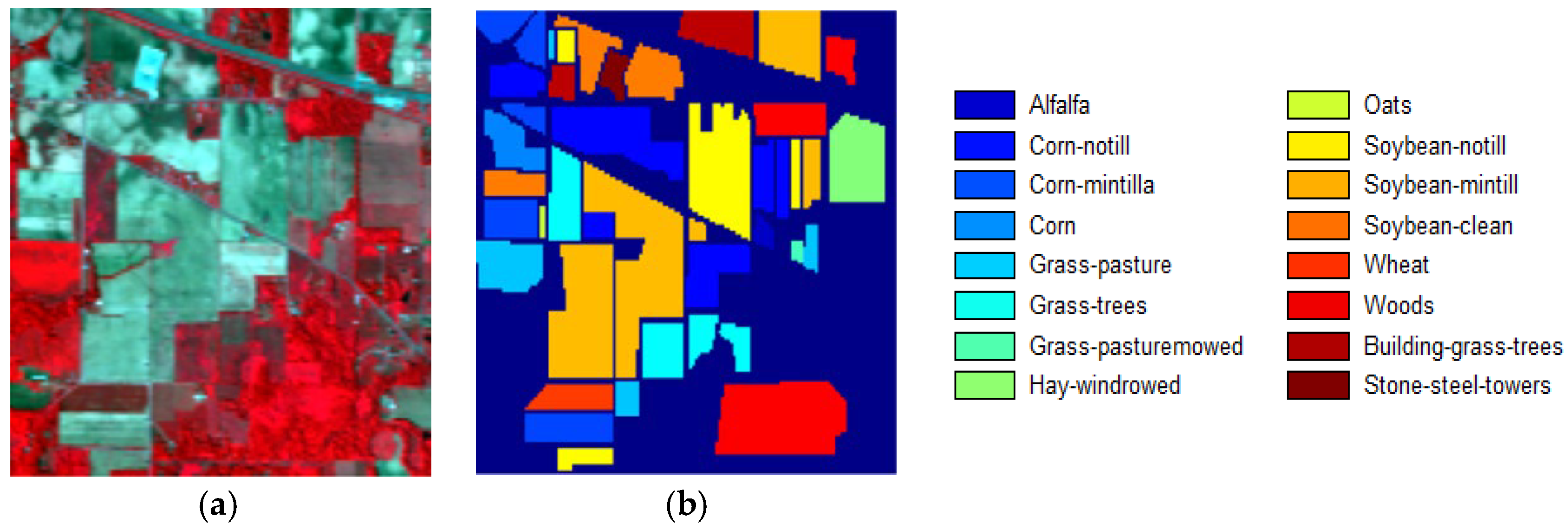
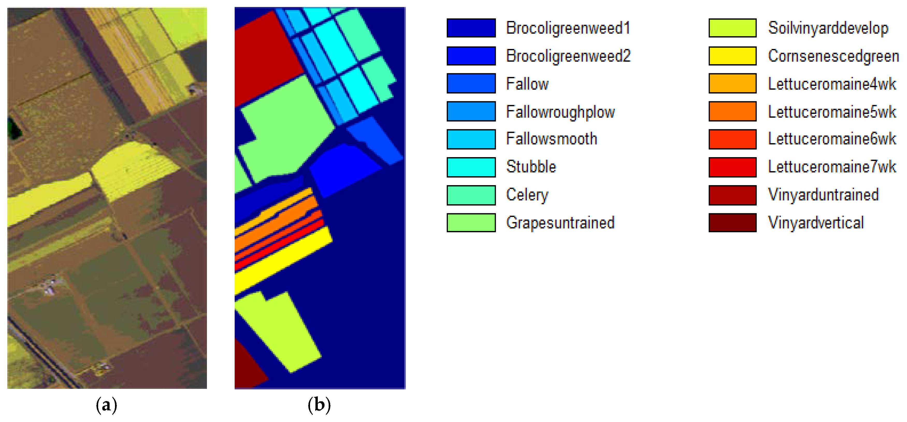
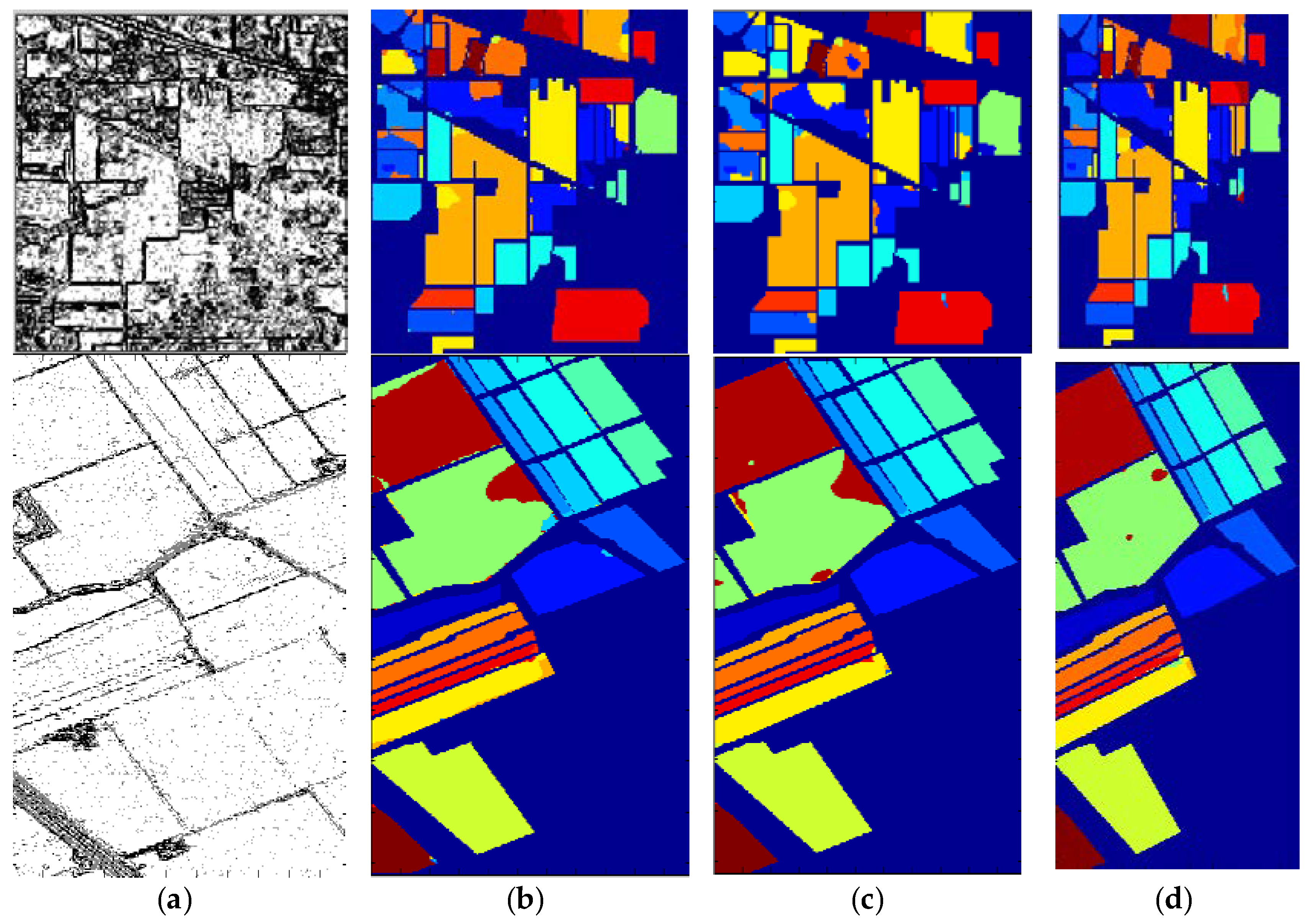
3.1. Datasets and Classification Results

The Indian Pines image was captured at the Indian Pines test station in northwestern Indiana, United States of America (USA), in 1992. The scene is composed of crops, forests, and other natural perennial vegetation. It has 220 successive spectral channels that range from 400 nm to 2500 nm and 145 pixels by 145 pixels with a spatial resolution of 20 m/pixel. Owing to the atmospheric water absorption, the spectral bands 104–108, 150–163, and 220 are removed to prevent them from affecting the classification performance, resulting in 200 available spectral bands. A total of 16 classes of terrestrial objects are available in the ground-truth map. The false color composition image and ground truth of the Indian Pines dataset are shown in Figure 1.
The Salinas dataset was gathered by the AVIRIS sensor over the Salinas Valley in California, USA, with a geometric resolution of 3.7 m per pixel. The size of the Salinas image is 512 × 217 × 224, where 20 water absorption spectral bands with insufficient information were removed; thus 204 available spectral bands remained. A total of 16 classes of ground-truth are included in the reference image. Figure 2 depicts the false-color composite image and the ground-truth image of the Salinas dataset.
These two hyperspectral datasets are available from http://www.ehu.eus/ccwintco/index.php/Hyperspectral_Remote_Sensing_Scenes.
Based on the initial training sets and the proposed method, the classification results on the Indian Pines and Salinas datasets are reported in Table 1. For Indian Pines dataset, the best classification accuracy over OA is 91.18% on average, in the case of randomly selecting 15 instances from each class. In other words, this result is obtained from approximately 2.3% of the total labeled samples. The classification accuracy of this dataset may not be as high as anticipated because of its serious data disequilibrium. The perfect classification result on the Salinas dataset has been obtained even if only 0.15% of the samples are labeled (label 5 samples per class). This fact successfully demonstrates that the proposal is valid for HSI classification with very small training sets. Table 1 also indicates that the classification result provided using the LMPNN classifier is better than that achieved by applying the KNN method of pre-classification. It is noteworthy that the application of post-processing technology has significantly improved the classification result. The classification accuracy and the standard deviation of each class in the Indian Pines and Salinas datasets are recorded in Table 2 and Table 3, respectively. In Figure 3, we present the classification map obtained by PMLMP with different numbers of labeled sample.

3.2. Comparative Tests

To objectively compare our method with other competitive approaches, it is necessary to select the same dataset, labeling proportion, and methods related to the MLR technique. Therefore, we have performed comparative experiments on the Indian Pines and Salinas datasets for the case of randomly selecting 15 instances from each class. Table 4 shows the comparison results provided by MLR, MLR-MLL (multilevel logistic prior) [43], ppMLR, prMLRpr [16] approaches, and the proposed method. For the Indian Pines dataset, no significant change is shown in the classification accuracy obtained by ppMLRpr and PMLMP. A similar classification result (OA = 90.44%) has also been achieved by the MLR + KNN + SNI method [2]. However, for the Salinas dataset, the method we proposed provides a perfect classification result. The classification accuracy of this study is approximately 4% higher than that of the ppMLRpr algorithm. Table 1 and Table 4 show that the results obtained by the PMLM and PMLMP techniques are still higher than those acquired by the ppMLRpr method, even for the random selection of five samples per category. This fact fully demonstrates the validity of the proposed method for remote-sensing data classification, even for the case of a small sample set.
Table 5 displays the superiority of using the Roberts cross operator over the Sobel filter in the proposed algorithm. For the random selection of 15 samples per class, the classification accuracies on both datasets have improved by at least 1%. This explains, to some extent, the rationality of the replacement scheme in pre-processing and post-processing.

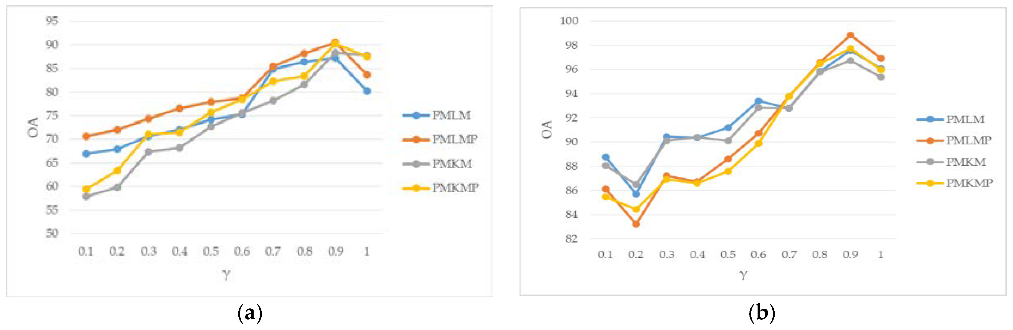
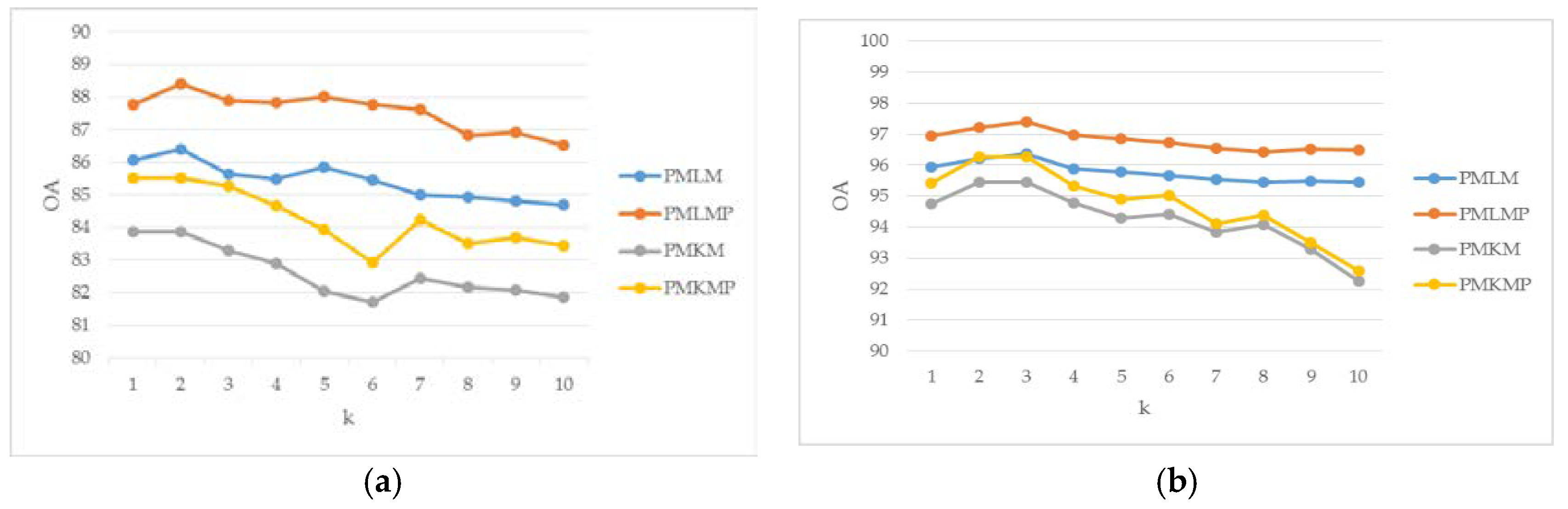
3.3. Parameter Analysis

It is arduous to select the optimal parameter value in the classification algorithm. Our experience shows that the classification result generally depends on the selection of the parameter value. Figure 4 reflects the correlation between the classification result and parameter γ used in the relaxation strategy. The classification accuracy becomes increasingly better with the increase in γ. The best classification result is achieved with γ = 0.9, which is consistent with Li’s selection [16]. This shows that the selection of parameter γ is independent of the selection of the operators. Parameter γ = 1 means that the boundary operator has complete control while the smoothness is ignored. Figure 3a shows that the use of the boundary operator cannot determine all the boundaries accurately; therefore, the classification accuracy is reduced.
Generally, the choice of the k value has a direct effect on the classification result provided by the LMPNN classifier or algorithms related to this classifier. To achieve the ideal classification result, it is clear that different k values need to be prespecified for different datasets. Figure 5 shows the relationship between the classification accuracy and k value in two datasets. Although the classification result has a slight change with the increase in k, we can still obtain the best result. Thus, in our algorithm, k is 2 for the Indian Pines dataset and 3 for the Salinas dataset.

4. Conclusions

In this study, we developed a novel semi-supervised method for HSI classification based on the DPR strategy and pre-classification technique. Using the DPR strategy in pre-processing and post-processing achieves the purpose of denoising and improving the classification accuracy, respectively. The pre-classification technique is aimed to address the problem of limited training samples in a semi-supervised classification. Our experimental results using the Indian Pines and Salinas datasets show that in the DPR strategy, the substitution of the Roberts cross operator with the Sobel filter can yield better classification results. The comparative test results show that the proposed method is superior to several existing methods. In particular, the proposal can provide perfect classification results for limited training samples.

Author Contributions

D.H., F.X. and D.L. conceived of and designed the experiments; D.H. and F.L. performed the experiments; J.Y., D.L., and D.H. analyzed the data and developed the graphs and tables; and F.L. and F.X. wrote the paper.

Funding

This work was supported by the National Natural Science Foundation of China (grants 41771178 and 61772252).

Acknowledgments

In this section you can acknowledge any support given which is not covered by the author contribution or funding sections. This may include administrative and technical support, or donations in kind (e.g., materials used for experiments).

Conflicts of Interest

The authors declare no conflict of interest.

References

  1. Wilson, T.; Felt, R. Hyperspectral remote sensing technology (HRST) program. In Proceedings of the 1998 IEEE Aerospace Conference, Snowmass at Aspen, CO, USA, 28 March 1998; pp. 193–200. [Google Scholar]
  2. Tan, K.; Hua, J.; Li, J.; Du, P. A novel semi-supervised hyperspectral image classification approach based on spatial neighborhood information and classifier combination. ISPRS J. Photogramm. Remote Sens. 2015, 105, 19–29. [Google Scholar] [CrossRef]
  3. Paoli, A.; Melgani, F.; Pasolli, E. Clustering of hyperspectral images based on multi-objective particle swarm optimization. IEEE Trans. Geosci. Remote Sens. 2009, 47, 4175–4188. [Google Scholar] [CrossRef]
  4. Wu, J. Unsupervised intrusion feature selection based genetic algorithm and FCM. In Lecture Notes in Electrical Engineering; Springer: London, UK, 2012; Volume 154, pp. 1005–1012. [Google Scholar]
  5. Camps-Valls, G.; Gomez-Chova, L.; Munoz-Mari, J.; Rojo-Alvare, J.L.; Martinez-Ramon, M. Kernel-based framework for multitemporal and multisource remote sensing data classification and change detection. IEEE Trans. Geosci. Remote Sens. 2008, 46, 1822–1835. [Google Scholar] [CrossRef] [Green Version]
  6. Bioucas-Dias, J.; Plaza, A.; Camps-Valls, G.; Scheunders, P.; Nasrabadi, N.; Chanussot, J. Hyperspectral remote sensing data analysis and future challenges. IEEE Geosci. Remote Sens. Mag. 2013, 1, 6–36. [Google Scholar] [CrossRef]
  7. Ghamisi, P.; Hofle, B. LiDAR Data Classification using Extinction prolfies and a composite kernel support vector machine. IEEE Geosci. Remote Sens. Lett. 2017, 14, 659–663. [Google Scholar] [CrossRef]
  8. Feng, J.; Jiao, L.C.; Zhang, X.; Sun, T. Hyperspectral band selection based on trivariate mutual information and clonal selection. IEEE Trans. Geosci. Remote Sens. 2014, 57, 4092–4105. [Google Scholar] [CrossRef]
  9. Feng, J.; Jiao, L.; Liu, F.; Sun, T.; Zhang, X. Unsupervised feature selection based on maximum information and minimum redundancy for hyperspectral images. Pattern Recognit. 2016, 51, 295–309. [Google Scholar] [CrossRef]
  10. Tobler, W. Computer movie simulating urban growth in the Detroit region. Econ. Geogr. 1970, 46, 234–240. [Google Scholar] [CrossRef]
  11. Heras, D.; Argüello, F.; Quesada-Barriuso, P. Exploring ELM-based spatial–spectral classification of hyperspectral images. Int. J. Remote Sens. 2014, 35, 401–423. [Google Scholar] [CrossRef]
  12. Franchi, G.; Angulo, J. Morphological principal component analysis for hyperspectral image analysis. ISPRS Int. J. Geo-Inf. 2016, 5, 83. [Google Scholar] [CrossRef]
  13. Ghamisi, P.; Dalla Mura, M.; Benediktsson, J. A Survey on Spectral-spatial classification techniques based on attribute profiles. IEEE Trans. Geos. Remote Sens. 2015, 53, 2335–2353. [Google Scholar] [CrossRef]
  14. Liu, J.; Xiao, Z.; Chen, Y.; Yang, J. Spatial-spectral graph regularized kernel sparse representation for hyperspectral image classification. ISPRS Int. J. Geo-Inf. 2017, 6, 258. [Google Scholar] [CrossRef]
  15. Paul, S.; Nagesh Kumar, D. Spectral-spatial classification of hyperspectral data with mutual information based segmented stacked autoencoder approach. ISPRS J. Photogramm. Remote Sens. 2018, 138, 265–280. [Google Scholar] [CrossRef]
  16. Li, J.; Khodadadzadeh, M.; Plaza, A.; Jia, X.; Bioucas-Dias, J.M. A discontinuity preserving relaxation scheme for spectral–spatial hyperspectral image classification. IEEE J. Sel. Top. Appl. Earth Obs. Remote Sens. 2017, 9, 625–639. [Google Scholar] [CrossRef]
  17. Yu, H.; Gao, L.; Li, J.; Li, S.S.; Zhang, B.; Benediktsson, J.A. Spectral-spatial hyperspectral image classification using subspace-based support vector machines and adaptive Markov random fields. Remote Sens. 2016, 8, 355. [Google Scholar] [CrossRef]
  18. Li, H.; Zheng, H.; Han, C.; Wang, H.; Miao, M. Onboard spectral and spatial cloud detection for hyperspectral remote sensing images. Remote Sens. 2018, 10, 152. [Google Scholar] [CrossRef]
  19. Ghamisi, P.; Benediktsson, J.A.; Ulfarsson, M.O. Spectral–spatial classification of hyperspectral images based on hidden Markov random fields. IEEE Trans. Geosci. Remote Sens. 2014, 52, 2565–2574. [Google Scholar] [CrossRef]
  20. Li, W.; Prasad, S.; Fowler, J.E. Hyperspectral image classification using gaussian mixture models and Markov random fields. IEEE Geosci. Remote Sens. Lett. 2013, 11, 153–157. [Google Scholar] [CrossRef]
  21. Sun, L.; Wu, Z.; Liu, J.; Xiao, L.; Wei, Z. Supervised spectral–spatial hyperspectral image classification with weighted Markov random fields. IEEE Trans. Geosci. Remote Sens. 2015, 53, 1490–1503. [Google Scholar] [CrossRef]
  22. Deng, W.; Iyengar, S.S. A New Probabilistic Relaxation Scheme and Its Application to Edge Detection. IEEE Trans. Pattern Anal. Mach. Intell. 1996, 18, 432–437. [Google Scholar] [CrossRef]
  23. Wang, L.; Dai, Q.; Huang, X. spatial regularization of pixel-based classification maps by a two-step MRF method. In Proceedings of the IEEE International Geoscience and Remote Sensing Symposium (IGARSS), Beijing, China, 10–15 July 2016; pp. 2407–2410. [Google Scholar]
  24. Gao, Q.; Lim, S.; Jia, X. Hyperspectral image classification using joint sparse model and discontinuity preserving relaxation. IEEE Geosci. Remote Sens. Lett. 2017, 99, 78–82. [Google Scholar] [CrossRef]
  25. Lin, Z.; Yan, L. A support vector machine classifier based on a new kernel function model for hyperspectral data. Mapp. Sci. Remote Sens. 2016, 53, 85–101. [Google Scholar] [CrossRef]
  26. Prabhakar, T.V.N.; Xavier, G.; Geetha, P.; Soman, K.P. Spatial preprocessing based multinomial logistic regression for hyperspectral image classification. Procedia Comput. Sci. 2015, 46, 1817–1826. [Google Scholar] [CrossRef]
  27. Khodadadzadeh, M.; Li, J.; Plaza, A.; Bioucas-Dias, J.M. A subspace-based multinomial logistic regression for hyperspectral image classification. IEEE Geosci. Remote Sens. Lett. 2014, 11, 2105–2109. [Google Scholar] [CrossRef]
  28. Ma, L.; Crawford, M.M.; Tian, J. Local manifold learning-based k-nearest-neighbor for hyperspectral image classification. IEEE Trans. Geosci. Remote Sens. 2010, 48, 4099–4109. [Google Scholar] [CrossRef]
  29. Denoeux, T. A k-nearest neighbor classification rule based on Dempster-Shafer theory. IEEE Trans. Syst. Man Cybern. 2008, 25, 804–813. [Google Scholar] [CrossRef]
  30. Gou, J.; Zhan, Y.; Rao, Y.; Shen, X.; Wang, X.; He, W. Improved pseudo nearest neighbor classification. Knowl.-Based Syst. 2014, 70, 361–375. [Google Scholar] [CrossRef]
  31. Zhang, Q.; Zhang, W.; Sun, Y.; Hu, P.; Tu, K. Detection of cold injury in peaches by hyperspectral reflectance imaging and artificial neural network. Food Chem. 2016, 192, 134–141. [Google Scholar]
  32. Ahmed, A.; Duran, O.; Zweiri, Y.; Smith, M. Hybrid spectral unmixing: Using artificial neural networks for linear/non-linear switching. Remote Sens. 2017, 9, 775. [Google Scholar] [CrossRef]
  33. Mitani, Y.; Hamamoto, Y. A local mean-based nonparametric classifier. Pattern Recognit. Lett. 2006, 27, 1151–1159. [Google Scholar] [CrossRef]
  34. Zeng, Y.; Yang, Y.; Zhao, L. Pseudo nearest neighbor rule for pattern classification. Expert Syst. Appl. 2009, 36, 3587–3595. [Google Scholar] [CrossRef]
  35. Tarabalka, Y.; Fauvel, M.; Chanussot, J.; Benediktsson, J.A. SVM and MRF-based method for accurate classification of hyperspectral images. IEEE Geosci. Remote Sens. Lett. 2010, 7, 736–740. [Google Scholar] [CrossRef]
  36. Li, J.; Bioucas-Dias, J.; Plaza, A. Spectral–spatial hyperspectral image segmentation using subspace multinomial logistic regression and markov random fields. IEEE Trans. Geosci. Remote Sens. 2012, 50, 809–814. [Google Scholar] [CrossRef]
  37. Roberts, L.G. Machine Perception of Three-Dimensional Solids; Outstanding Dissertations in the Computer Sciences; Garland Publishing: New York, NY, USA, 1963. [Google Scholar]
  38. Böning, D. Multinomial logistic regression algorithm. Annu. Inst. Stat. Math. 1992, 44, 197–200. [Google Scholar] [CrossRef]
  39. Li, J.; Bioucas-Dias, J.; Plaza, A. Spectral–spatial classification of hyperspectral data using loopy belief propagation and active learning. IEEE Trans. Geosci. Remote Sens. 2013, 51, 844–856. [Google Scholar] [CrossRef]
  40. Camps-Valls, G.; Bruzzone, L. Kernel-based methods for hyperspectral image classification. IEEE Trans. Geosci. Remote Sens. 2005, 43, 1351–1362. [Google Scholar] [CrossRef] [Green Version]
  41. Cover, T.M.; Hart, P.E. Nearest neighbor pattern classification. IEEE Trans. Inf. Theory 1967, 13, 21–27. [Google Scholar] [CrossRef] [Green Version]
  42. Dudani, S.A. The distance-weighted k-nearest neighbor rule. IEEE Trans. Syst. Man Cybern. 1976, 6, 325–327. [Google Scholar] [CrossRef]
  43. Li, J.; Bioucas-Dias, J.; Plaza, A. Semi-supervised hyperspectral image segmentation using multinomial logistic regression with active learning. IEEE Trans. Geosci. Remote Sens. 2010, 48, 4085–4098. [Google Scholar]
Figure 1. Indian Pines dataset. (a) False color composition; (b) Ground-truth.
Ijgi 07 00284 g001
Figure 2. Salinas dataset. (a) False color composition; (b) Ground-truth.
Ijgi 07 00284 g002
Figure 3. Discontinuity map and classification map obtained by pre-processing + MLRsub + the local mean-based pseudo nearest neighbor (LMPNN) rule + multinomial logistic regression with subspace projection (MLRsub) + post-processing (PMLMP) with different numbers of labeled samples. The above row is for the Indian Pines dataset and the below for the Salinas dataset. (a) Discontinuity map. (bd) classification map with 5, 10, and 15 labeled samples per class, respectively.
Ijgi 07 00284 g003
Figure 4. A line chart of classification results varying with relaxation parameter on two hyperspectral images (HSIs). (a) Indian Pines dataset; (b) Salinas dataset.
Ijgi 07 00284 g004
Figure 5. The relation between the classification result and parameter k. (a) Indian Pines; (b) Salinas.
Ijgi 07 00284 g005
Table 1. Classification results of the Indian Pines and Salinas datasets by different methods with different label proportions.
DatasetMethod51015
OA (%)KC (%)OA (%)KC (%)OA (%)KC (%)
Indian PinesPMKM74.85 ± 1.1071.55 ± 1.4384.53 ± 1.6982.48 ± 2.1388.73 ± 3.9987.22 ± 4.91
PMLM75.05 ± 3.5771.87 ± 4.4884.57 ± 2.1282.55 ± 2.6788.95 ± 1.2587.48 ± 1.59
PMKMP76.89 ± 1.3673.80 ± 1.5686.45 ± 1.0884.64 ± 1.3690.46 ± 4.1089.17 ± 5.14
PMLMP77.23 ± 2.8574.27 ± 3.7186.69 ± 1.3984.92 ± 1.7291.18 ± 2.3089.98 ± 3.90
SalinasPMKM92.16 ± 1.0691.30 ± 1.2895.11 ± 5.7694.58 ± 7.0896.77 ± 1.2996.41 ± 1.59
PMLM95.22 ± 3.6594.69 ± 4.4896.02 ± 6.8495.58 ± 8.4597.12 ± 2.5096.80 ± 3.08
PMKMP93.05 ± 1.6892.28 ± 2.0495.90 ± 4.0295.45 ± 4.9397.42 ± 5.3097.13 ± 6.55
PMLMP96.00 ± 2.9895.56 ± 3.6696.82 ± 4.0096.46 ± 4.9997.96 ± 3.8397.74 ± 4.73
Table 2. Classification accuracy over overall accuracy (OA (%)) and standard deviations for each class in the Indian Pines dataset.
51015
PMKMPMLMPMKMPPMLMPPMKMPMLMPMKMPPMLMPPMKMPMLMPMKMPPMLMP
Alfalfa (46)93.70 ± 1.90 95.22 ± 2.00 93.48 ± 1.7792.39 ± 1.8594.35 ± 2.3494.35 ± 2.9394.13 ± 1.4794.35 ± 2.0697.61 ± 2.1696.09 ± 1.7195.00 ± 2.2493.91 ± 1.05
Corn-no till (1428)43.10 ± 10.25 48.40 ± 11.81 45.87 ± 13.4551.23 ± 12.0472.25 ± 4.2268.93 ± 6.2968.12 ± 10.3268.93 ± 5.2676.67 ± 5.4580.08 ± 5.3680.86 ± 5.9084.46 ± 7.66
Corn-min till (830)60.18 ± 12.57 60.80 ± 13.3663.00 ± 16.6268.82 ± 13.6981.14 ± 8.8678.88 ± 5.7285.70 ± 8.5878.88 ± 5.8180.48 ± 9.8283.94 ± 7.4385.11 ± 8.1285.16 ± 9.20
Corn (237)85.15 ± 8.05 75.61 ± 17.6984.51 ± 8.7778.99 ± 19.8183.88 ± 11.3988.44 ± 9.4384.94 ± 11.3888.44 ± 7.7890.89 ± 4.5390.55 ± 4.3690.51 ± 4.8589.79 ± 6.37
Grass-pasture (483)75.01 ± 8.56 79.05 ± 9.3676.87 ± 11.0073.31 ± 19.4289.65 ± 3.6287.74 ± 4.9891.78 ± 3.8587.74 ± 4.2491.16 ± 4.0789.23 ± 9.0592.63 ± 3.7991.93 ± 4.33
Grass-trees (730)99.74 ± 0.56 99.49 ± 0.5099.96 ± 0.1098.59 ± 2.8899.62 ± 0.6498.84 ± 2.0399.82 ± 0.3598.84 ± 0.5999.62 ± 0.6199.71 ± 0.4699.99 ± 0.0099.99 ± 0.00
Grass-pasture-mowed (28)99.64 ± 1.13 100.00 ± 0.0098.21 ± 3.86100.00 ± 0.00100.00 ± 0.0098.57 ± 4.5287.14 ± 16.4398.57 ± 14.6099.29 ± 2.26100.00 ± 0.0092.50 ± 10.1394.29 ± 12.42
Hay-windrowed (478)93.39 ± 3.91 93.77 ± 3.6595.31 ± 2.6495.42 ± 3.5294.85 ± 4.2692.76 ± 12.5195.77 ± 3.6792.76 ± 12.8596.51 ± 4.8196.99 ± 3.1894.21 ± 0.8198.37 ± 7.93
Oats (20)100.00 ± 0.00 100.00 ± 0.00100.00 ± 0.00100.00 ± 0.00100.00 ± 0.00100.00 ± 0.00100.00 ± 0.00100.00 ± 0.00100.00 ± 0.00100.00 ± 0.00100.00 ± 0.00100.00 ± 0.00
Soybean-no till (972)78.77 ± 11.50 82.35 ± 8.1980.94 ± 12.0183.08 ± 9.7789.87 ± 7.0286.77 ± 5.3991.97 ± 6.6186.77 ± 4.6492.12 ± 5.7491.87 ± 5.1692.87 ± 5.1393.55 ± 5.62
Soybean-min till (2455)75.82 ± 3.87 71.60 ± 5.5977.30 ± 5.3173.57 ± 5.3378.37 ± 4.9879.97 ± 4.2582.65 ± 2.6279.97 ± 5.0785.62 ± 3.1385.92 ± 2.9688.47 ± 3.5888.21 ± 3.29
Soybean-clean (593)69.12 ± 8.33 59.98 ± 15.9966.31 ± 16.1166.58 ± 7.4667.93 ± 14.2980.12 ± 10.2173.66 ± 14.8380.12 ± 10.3287.74 ± 7.7482.56 ± 9.5283.93 ± 6.8984.65 ± 10.30
Wheat (205)99.27 ± 0.81 99.32 ± 0.5799.66 ± 0.3399.61 ± 0.2099.46 ± 0.9699.46 ± 0.7499.80 ± 0.2499.46 ± 0.2099.80 ± 0.3599.46 ± 0.7199.66 ± 0.2099.61 ± 0.24
Woods (1265)90.84 ± 10.19 92.51 ± 4.8994.33 ± 7.5594.96 ± 5.2998.09 ± 3.1297.64 ± 3.7097.95 ± 3.2897.64 ± 3.1097.33 ± 2.8296.93 ± 2.8198.58 ± 2.1798.63 ± 2.17
Buildings-Grass-Trees-Drives (386)73.76 ± 13.78 79.72 ± 7.9475.67 ± 14.7479.27 ± 13.6791.01 ± 6.3290.78 ± 7.9995.13 ± 7.8390.78 ± 8.9594.84 ± 4.1697.98 ± 1.0295.39 ± 4.1797.93 ± 6.57
Stone-Steel-Towers (93)96.24 ± 2.83 93.87 ± 4.9795.16 ± 4.1991.72 ± 4.5196.67 ± 3.5394.84 ± 2.5793.01 ± 5.2794.84 ± 4.1895.59 ± 2.9793.66 ± 4.1093.44 ± 3.5092.69 ± 3.77
Table 3. Classification accuracy over OA (%) and its standard deviations for each class in the Salinas dataset.
51015
PMKMPMLMPMKMPPMLMPPMKMPMLMPMKMPPMLMPPMKMPMLMPMKMPPMLMP
Brocoli_green_weeds_1 (2009)99.67 ± 0.5699.27 ± 1.8799.78 ± 0.4499.40 ± 1.7599.76 ± 0.2899.54 ± 0.6999.93 ± 0.2299.69 ± 0.5199.72 ± 0.4299.79 ± 0.3799.67 ± 0.4899.92 ± 0.26
Brocoli_green_weeds_2 (3726)99.90 ± 0.1799.81 ± 0.30100.00 ± 0.0099.97 ± 0.0099.82 ± 0.4499.92 ± 0.1499.97 ± 0.10100.00 ± 0.0099.98 ± 0.0099.92 ± 0.17100.00 ± 0.0099.99 ± 0.00
Fallow (1976)93.84 ± 9.6797.02 ± 3.5495.29 ± 9.8698.07 ± 3.0299.89 ± 0.2299.35 ± 1.1599.61 ± 1.2099.72 ± 0.5799.89 ± 0.2299.92 ± 0.1499.98 ± 0.0099.98 ± 0.00
Fallow-rough-plow (1394)98.27 ± 0.8397.70 ± 1.7198.21 ± 1.2097.67 ± 2.5298.42 ± 0.3298.01 ± 0.6398.68 ± 0.7297.96 ± 1.1697.77 ± 0.8498.14 ± 0.5497.71 ± 1.4798.12 ± 1.01
Fallow-smooth (2678)95.81 ± 4.4896.52 ± 2.3697.68 ± 3.6697.45 ± 2.0397.98 ± 1.0898.85 ± 1.2199.01 ± 0.8299.19 ± 0.8398.69 ± 0.7797.66 ± 1.6699.28 ± 0.4798.41 ± 1.57
Stubble (3959)99.74 ± 0.2299.78 ± 0.2099.96 ± 0.0099.96 ± 0.0099.78 ± 0.2499.73 ± 0.2499.97 ± 0.0099.96 ± 0.0099.88 ± 0.0099.86 ± 0.1099.96 ± 0.0099.97 ± 0.00
Celery (3579)99.79 ± 0.1099.80 ± 0.1099.94 ± 0.0099.96 ± 0.0099.84 ± 0.1099.80 ± 0.1099.95 ± 0.0099.95 ± 0.0099.82 ± 0.1499.81 ± 0.1499.95 ± 0.0099.94 ± 0.00
Grapes-untrained (11271)78.22 ± 8.0986.79 ± 2.8279.95 ± 8.3388.78 ± 2.4882.72 ± 3.0087.91 ± 1.2985.02 ± 2.8990.20 ± 0.8189.55 ± 1.6284.54 ± 5.1891.46 ± 1.1686.69 ± 5.73
Soil-vineyard-develop (6203)99.49 ± 0.7499.65 ± 0.6799.76 ± 0.5599.84 ± 0.3999.99 ± 0.0099.95 ± 0.14100.00 ± 0.0099.99 ± 0.0099.99 ± 0.0099.98 ± 0.00100.00 ± 0.00100.00 ± 0.00
Corn-senesced-green-weeds (3278)85.61 ± 5.2889.99 ± 2.9487.30 ± 5.6891.35 ± 2.7492.30 ± 3.6892.72 ± 2.5194.29 ± 2.7993.49 ± 2.2594.47 ± 1.6592.46 ± 6.5994.96 ± 1.6092.13 ± 7.74
Lettuce_romaine_4weeks (1068)99.30 ± 0.6299.56 ± 0.5699.65 ± 0.9099.78 ± 0.4499.12 ± 0.8899.64 ± 0.3599.50 ± 0.8699.87 ± 0.3598.90 ± 1.1599.54 ± 0.6999.77 ± 0.36100 ± 0.00
Lettuce_romaine_5weeks (1927)97.37 ± 4.5898.83 ± 2.1497.25 ± 5.0698.94 ± 1.8398.52 ± 2.3299.69 ± 0.3399.24 ± 1.5099.77 ± 0.2699.75 ± 0.3799.91 ± 0.1499.68 ± 0.3799.83 ± 0.24
Lettuce_romaine_6weeks (916)98.84 ± 1.3697.67 ± 1.7998.12 ± 1.8596.62 ± 2.3299.34 ± 0.4799.04 ± 0.9698.40 ± 0.9998.22 ± 1.4699.42 ± 0.4998.89 ± 1.1498.58 ± 1.2498.72 ± 1.34
Lettuce_romaine_7weeks (1070)97.83 ± 1.2797.10 ± 3.4797.54 ± 1.9896.02 ± 4.9798.63 ± 0.6398.30 ± 1.1097.88 ± 1.1898.57 ± 1.1198.47 ± 0.8998.76 ± 0.8998.11 ± 1.3297.84 ± 2.33
Vineyard-untrained (7268)89.43 ± 7.6694.72 ± 2.1490.83 ± 7.5095.72 ± 1.9396.62 ± 2.5494.94 ± 1.8597.16 ± 2.0796.11 ± 2.2297.26 ± 1.6695.15 ± 5.3798.16 ± 1.7696.12 ± 4.9
Vineyard-vertical-trellis (1807)92.40 ± 5.6496.44 ± 3.5993.56 ± 5.1997.60 ± 3.0798.17 ± 1.0998.57 ± 0.9898.97 ± 0.8599.13 ± 0.7197.75 ± 3.1297.20 ± 2.9498.38 ± 2.8698.38 ± 2.6
Table 4. Comparison results of several methods on two hyperspectral datasets.
MethodIndian PineSalinas
OA (%)KC (%)OA (%)KC (%)
MLR64.30 ± 2.2960.03 ± 2.4585.28 ± 1.5183.67 ± 1.66
MLR-MLL75.09 ± 2.8672.03 ± 3.1089.02 ± 6.5487.80 ± 7.28
ppMLR88.36 ± 1.6786.88 ± 1.8693.30 ± 1.7092.56 ± 1.89
ppMLRpr91.05 ± 1.8789.87 ± 2.0993.79 ± 4.4693.11 ± 4.91
PMKM88.73 ± 3.9987.22 ± 4.9196.77 ± 1.2996.41 ± 1.59
PMLM88.95 ± 1.2587.48 ± 1.5997.12 ± 2.5096.80 ± 3.08
PMKMP90.46 ± 4.1089.17 ± 5.1497.42 ± 5.3097.13 ± 6.55
PMLMP91.18 ± 2.3089.98 ± 3.9097.96 ± 3.8397.74 ± 4.73
Table 5. Comparison results of using the Roberts cross operator and Sobel filter in our proposal.
MethodOperatorIndian PineSalinas
OA (%)KC (%)OA (%)KC (%)
PMKMSobel85.15 ± 0.8183.23 ± 0.96 95.70 ± 0.8495.23 ± 1.03
Roberts88.73 ± 2.0087.22 ± 2.4696.77 ± 0.6596.41 ± 0.80
PMKMPSobel86.95 ± 0.4985.23 ± 0.5996.60 ± 3.5596.22 ± 4.39
Roberts90.46 ± 2.0589.17 ± 2.5797.42 ± 2.6597.13 ± 3.28
PMLMSobel84.74 ± 0.7782.78 ± 0.9396.04 ± 1.2595.60 ± 1.54
Roberts88.95 ± 0.6387.48 ± 0.8097.12 ± 1.2596.80 ± 1.54
PMLMPSobel86.33 ± 0.8484.54 ± 1.0296.90 ± 0.8396.56 ± 1.00
Roberts91.18 ± 1.1589.98 ± 1.9597.96 ± 1.9297.74 ± 2.37

