Reduction Method for Mobile Laser Scanning Data


1
Institute of Geodesy, Faculty of Geodesy, Geospatial and Civil Engineering, University of Warmia and Mazury in Olsztyn, Oczapowski St. 1, 10-719 Olsztyn, Poland
2
Department of Civil, Environmental and Geodetic Engineering, The Ohio State University, 470 Hitchcock Hall, 2070 Neil Avenue, Columbus, OH 43210, USA
*
Author to whom correspondence should be addressed.
ISPRS Int. J. Geo-Inf. 2018, 7(7), 285; https://doi.org/10.3390/ijgi7070285
Submission received: 30 May 2018
/
Revised: 1 July 2018
/
Accepted: 19 July 2018
/
Published: 23 July 2018
Abstract
:Mobile Laser Scanning (MLS) technology acquires a huge volume of data in a very short time. In many cases, it is reasonable to reduce the size of the dataset with eliminating points in such a way that the datasets, after reduction, meet specific optimization criteria. Various methods exist to decrease the size of point cloud, such as raw data reduction, Digital Terrain Model (DTM) generalization or generation of regular grid. These methods have been successfully applied on data captured from Airborne Laser Scanning (ALS) and Terrestrial Laser Scanning (TLS), however, they have not been fully analyzed on data captured by an MLS system. The paper presents our new approach, called the Optimum Single MLS Dataset method (OptD-single-MLS), which is an algorithm for MLS data reduction. The tests were carried out in two variants: (1) for raw sensory measurements and (2) for a georeferenced 3D point cloud. We found that the OptD-single-MLS method provides a good solution in both variants; therefore, the choice of the reduction variant depends only on the user.
1. Introduction
Mobile Laser Scanning (MLS) systems typically consist of a laser scanner, a Global Positioning System (GPS) receiver, an Inertial Measurement Unit (IMU), and cameras installed on a platform. The platform is often a car, for example, an Sport Utility Vehicle (SUV), as seen in the studies by Kukko et al. [1,2], but the platform could be other moving vehicle in special applications, such as a marine platform [3]. Currently, the data collected with MLS is processed with algorithms embedded in a special software which is dedicated only to MLS data; in the case of the 3D point cloud, it has been developed for processing TLS or ALS data. It is important to use such software, which can show dynamic MLS data [4]. Usually, MLS is used to capture road, building, and railway infrastructures to create an inventory or for the reconstruction of existing communication networks [5].
A review of conventional MLS systems and their accuracy assessments can be found in studies by Hruza et al., Mikrut et al., and Barber et al. [6,7,8]. They used RTK-GPS (Real Time Kinematic) measurements to collect reference data on two test sites to validate the geometric accuracy of the Streetmapper MLS system. The focus was on elevation accuracy; however, only a few control points measured on white line markings on the road were used for the analysis of planimetric accuracy. Similar problems were studied by researchers at the University of California at Davis in the United States [9]. They used total station and TLS data to analyze the accuracy of MLS system. During that study, only the elevation accuracy was examined.
In the recent years, lower cost Light Detection and Ranging (LiDAR) systems, such as Velodyne’s VLP-16 and HDL-32 LiDAR scanners, have received attention from the mapping community. These sensors are primary used in autonomous vehicles (AV) or for security/surveillance, but they can be also applied in low-cost mapping systems, for instance, on Unmanned Aerial Vehicles (UAVs). In terms of data processing, Velodyne has introduced a new open source software called VeloView for real-time visualizing and processing of 3D data from its high-definition LiDAR (HDL) sensors. VeloView displays distance measurements from the LiDAR sensors as a point cloud and supports custom color maps of variables such as intensity-of-return, time, distance, calibrated reflectivities, azimuth, and laser echo id. The point cloud can be exported as XYZ data in comma-separated values (csv) format. 3D data acquired over a period of time as well as the featured playback mode allows users to display changes in the environment as a function of time [10].
In comparison to conventional MLS systems, one of the issues with these sensors is the lower spatial resolution. Nevertheless, these sensors can produce a large amount of data; accordingly, data reduction might be required to store the data efficiently. In addition, the affordable price will allow many users to map the environment not just from dedicated and expensive MLS systems but also capture data with AVs, sharing these data with other road users in real time.
Velodyne’s VLP-16 sensor can make a 360° scan with 0.6° angular resolution around the rotation axis and contains 16 laser diodes perpendicularly installed to the rotation plane, which enables 30° field of view (FOV) along this (vertical) direction with a 2° sensor separation. The Velodyne VLP-16 scanning rate of 10 Hz results in 0.1°–0.4°, with affective 0.2° average separation between consecutive shots of a single laser diode, which equals a linear separation around 10 cm at a scanning distance of 30 m.
The HDL-32 works similarly, but it has 32 lasers diodes with separation; therefore, the vertical field of view is 40°. The focus of this study is to reduce the size of the dataset captured by multiple Velodyne sensors installed on an SUV. In general, previous studies have shown that the data processing of ALS, TLS, and MLS is challenging due to the large amount of data [11]. However, a mapping project often has a particular interest, and this interest can be achieved using a reduced data, for instance, an assessment of the road condition can be achieved by creating cross-sections of the road [12] and data preparation for classification [13,14]. Such an approach saves time and affects the speed of work. The purpose of reducing the size of MLS measurement datasets can be understood in two ways. The first goal is to simplify (in terms of time-consuming calculations) the process of creating a numerical model (DTM or DEM—Digital Elevation Model) or to prepare a “lighter” dataset for a specific task or project. The second goal is to drastically reduce the number of points representing the resulting model, with a concern to its further use. The decrease the number of points in datasets can be achieved by conducting generation, model generalization, or data reduction. Generation decreases the dataset by resampling at certain grid point [15]. Model generalization simplifies the shape of the model, if such a model exists or can be created [16]. In contrast, data reduction allows for a reduction in the size of the dataset by carefully removing points. The selection of points to be deleted is not random but based on algorithmic considerations. The reduction of a dataset needs to be properly planned so that the dataset, following the reduction, meets the users’ requirements and the interest of the mapping project. Obviously, it is best if the result is the optimal solution for the adopted criteria. It can be achieved by using the Optimum Dataset (OptD) method [17,18].
This paper is the continuation of our ongoing effort to develop an efficient data reduction and presents the modification of the Optimum Dataset method, with one criterion for MLS data captured by Velodyne sensors (called OptD-single-MLS).
The modification includes two options:
- Option 1 processes non-georeferenced frames that can be (a) one frame or (b) all frames.
- Option 2 processes (c) the georeferenced 3D point cloud.
The paper presents the methodology of MLS data reduction and illustrates the principle operations of the OptD-single-MLS method. Then, the method is tested on LiDAR data captured by Velodyne sensors. The results of the processing were subjected to statistical-emiric analyzes.
2. Materials and Methods
Our previous method, which was called the Optimum Dataset method, is presented in Błaszczak-Bąk et al. [17,18,19]. The OptD method removes those points which do not have relevant effect on the terrain characteristics from a practical point of view. The accuracy analysis using DTMs has been presented in Błaszczak-Bąk et al. [17,18]. The OptD method uses linear object generalization methods, but the calculations are performed in a vertical plane which allows for accurate control of the elevation component. The generalization approach used in the OptD method is the Visvalingam-Whyatt (V-W) method proposed by Visvalingam and Whyatt [20] or the Douglas-Peucker (D-P) method proposed by Douglas and Peucker [21].
The OptD method can be performed in two variants:
- The OptD method with one criterion optimization called the OptD-single.
- The OptD method with multi criteria optimization called the OptD-multi.
In the OptD-single method, a dataset that meets one strictly defined condition is searched, e.g., the numbers of points in the reduced dataset, the percent of points that will remain in the dataset, the defined value of standard deviation, or any other parameters specified by the user. If the user opts to perform the processing by means of the OptD-multi, he will obtain several datasets, from which the best one can be chosen.
In this paper, the authors modified the OptD-single method to efficiently handle MLS data. The OptD-single-MLS method consists of the following steps [1]:
- step 1:
- Loading the points of the original dataset (N). We can choose: Option 1 with (a) one frame, (b) all frames for one Velodyne, or Option 2 with (c) georeferenced 3D point cloud.The details of each of the Options are shown in Figure 1.
- step 2:
- Establishing optimization criterion (f), e.g., numbers of points in reduced dataset, standard deviation for the dataset.
- step 3:
- The choice of initial width of strips (L). When choosing the appropriate strips width, some parameters (depends on the user) can be taken into consideration: the average distance between points in the measurement set as well as the distance between the strips, which depends directly on the type of measurement (here: LiDAR), and they are a consequence of the principle of LiDAR measurement. Another way the strip’s width determination can be performed is in an iterative process (it is changed with a fixed interval until a satisfactory solution is achieved).
- step 4:
- Dividing the original (input) dataset into measurement strips (nL).
- step 5:
- Selection of measurement points for each strip. An example of measurement strip is presented in Figure 2.
- step 6:
- Selecting the cartographic line generalization method, e.g. the D-P or V-W.
- step 7:
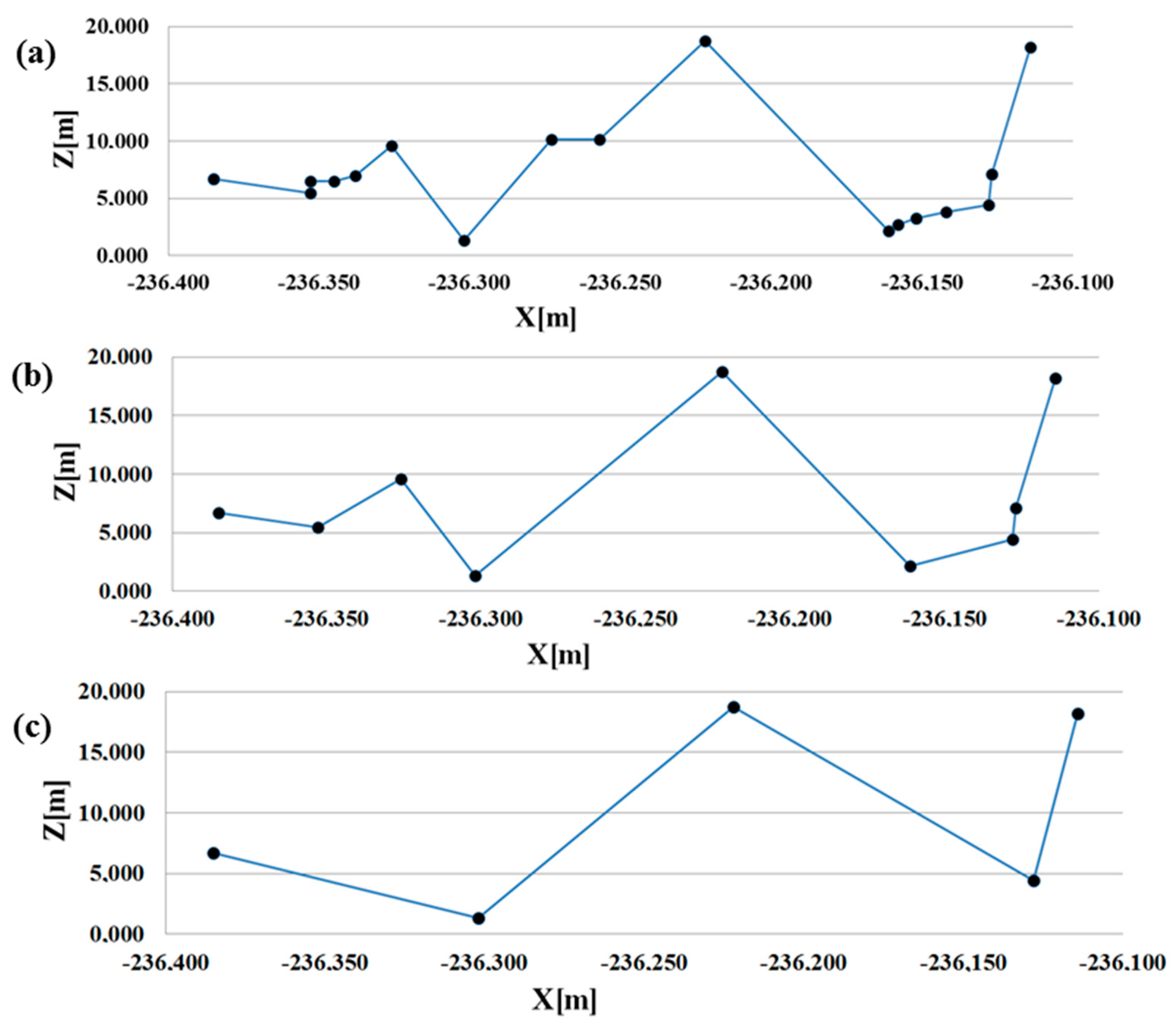
- Using the selected generalization method in the Y0Z plane (vertical plane) for each measurement strip and choosing the tolerance parameters in the selected generalization method. For the D-P method, it is a distance of tolerance (t). The initial value of the section is defined by the user; the following values are determined in an iterative process. Figure 3 illustrates the steps.
- step 8:
- Obtaining the reduced/output dataset with the number of M, where M < N.
- step 9:
- Verifying whether the obtained dataset in step 8 fits the specified criterion optimization. If so, the reduction process is completed, and the obtained set from step 8 is the optimal/the best dataset. If not, steps 6–9 are repeated in which the tolerance parameter is adjusted in step 7. If repeating steps 6–9 do not provide a solution, the width of the measurement strip in step 3 must be changed.
In summary, the OptD-single-MLS method uses the following parameters: f—optimization criterion; L—initial width of strips; nL—the number of measurement strips; t—tolerance for generalization algorithm; N—the number of points in the original dataset; and M—the number of points in the reduced dataset.
3. Sensors and Data Processing
MLS data was acquired during the Fourth International Working Week on Multi-Sensor Integration for Assured Navigation, 1–8 October 2017. The meeting took place at Ohio State University.
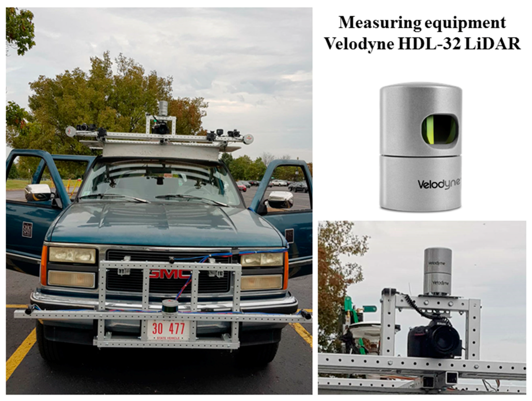
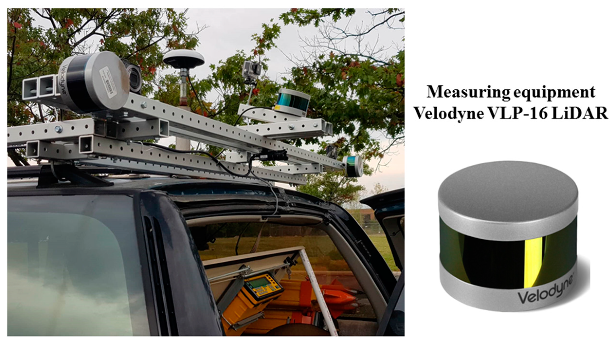
A van was used for data acquisition. One Velodyne HDL-32 on the front top and eight Velodyne VLP-16 on the side and rear of the vehicle were installed.
Velodyne HDL-32 LiDAR generates up to ~1.39 million points per second with ±2 cm accuracy. Velodyne VLP-16 LiDAR generates up to ~600 thousands points per second with ±3 cm accuracy.
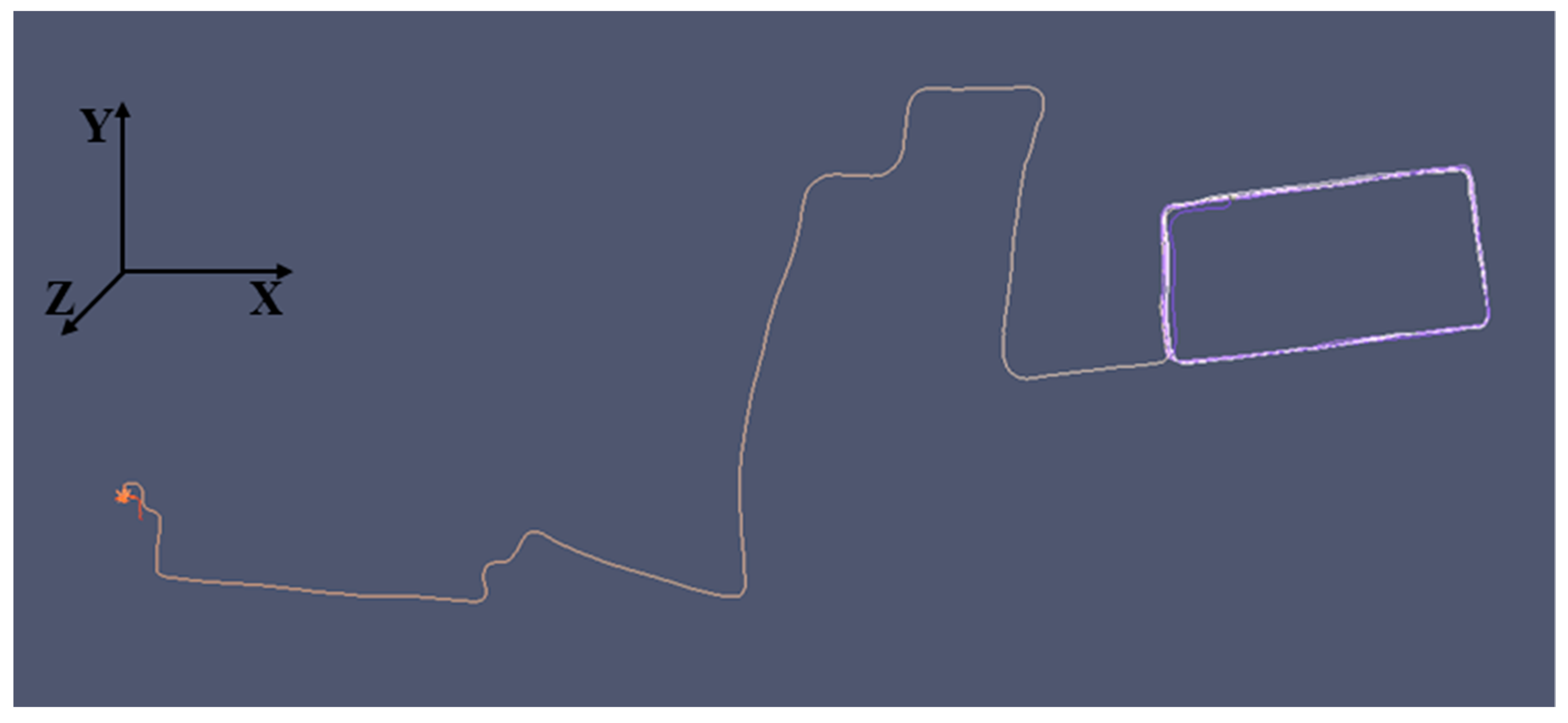
Figure 4 shows the vehicle with Velodyne HDL-32 LiDAR. The rear Velodyne VLP-16 LiDAR sensors are shown in Figure 5. Data was collected around the OSU campus; the trajectory can be seen in Figure 6.
The acquired point clouds from the LiDAR sensors were defined in the sensor’s coordinate system. To use the point cloud for option 2, the data should be georeferenced. Standard georeferencing of MLS data was based on the transformation from the scanner local coordinates to global coordinates using boresight parameters and navigation information from the on-board GPS and IMU [6,22].
4. Results
The OptD-single-MLS method was tested on MLS data. At stage 2 of the OptD-single-MLS method, the percentage of points in the output dataset was assumed as optimization criterion. In Option 1 (Figure 1), the OptD-single-MLS method was applied for two chosen frames, named Frame 1 and Frame 2.
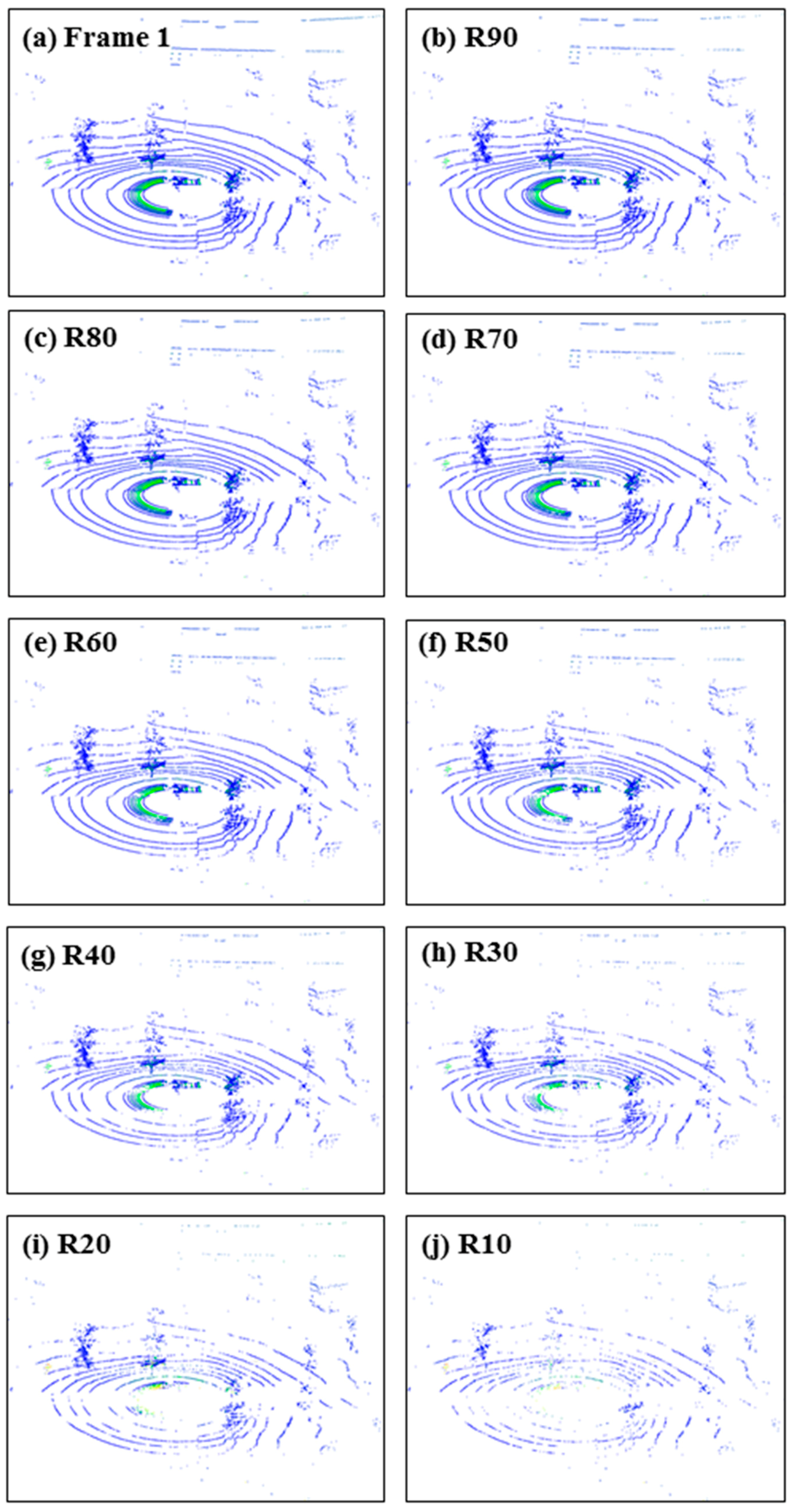
Figure 7a shows a point cloud of Frame 1; Figure 7b–j shows the reduced MLS data. The percentage of points to be left in the set after the reduction was chosen for the optimization criterion in the OptD-single-MLS method. Therefore, the reduced MLS data were named, respectively, Ri, where i denotes how many percent of points have been left in dataset after reduction i = 10, 20, ..., 90.
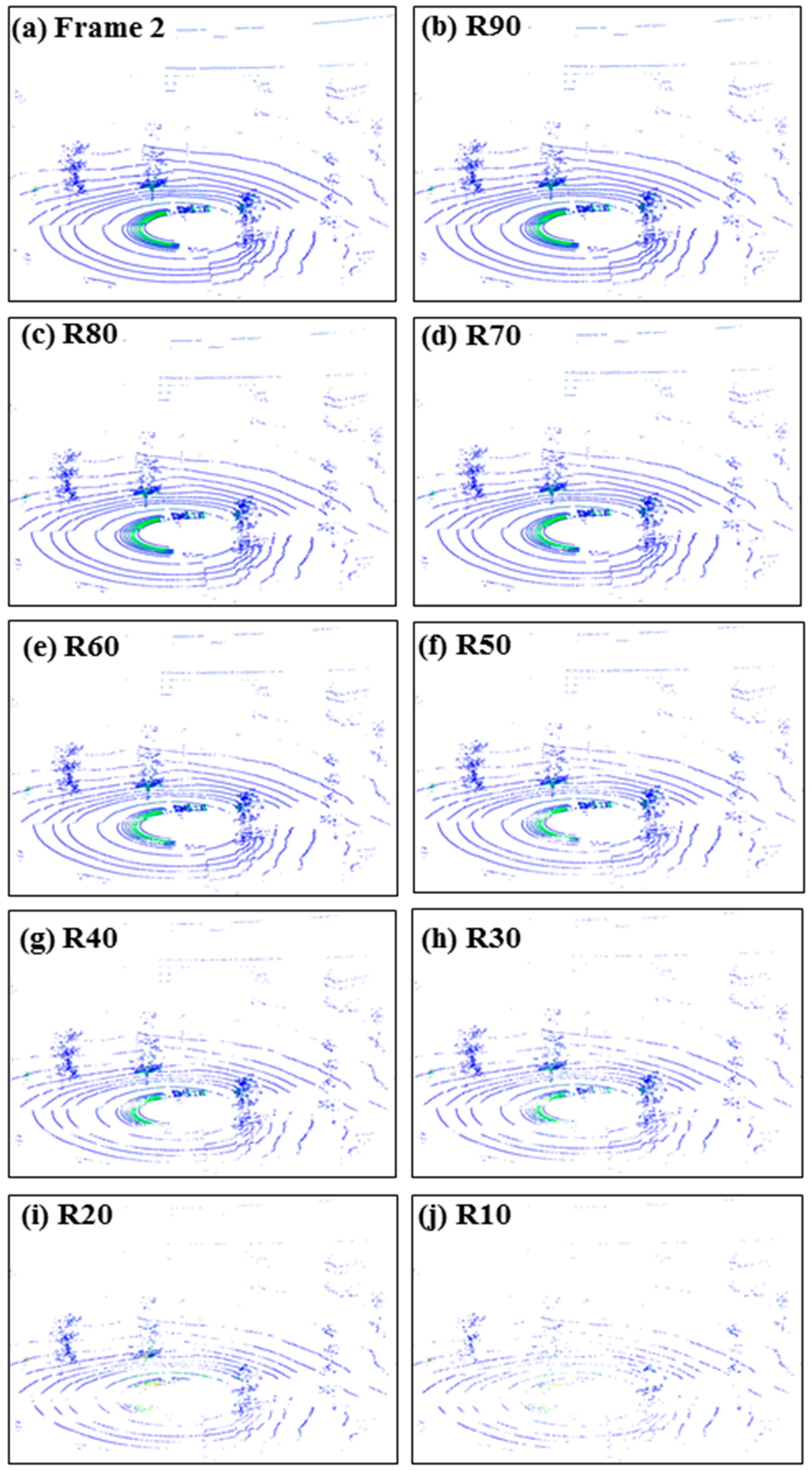
Figure 8a shows MLS data from Frame 2; Figure 8b–j shows the reduced point clouds. The same optimization criterion was used as for Frame 1.
The original dataset for Frame 1 and the derived datasets after OptD-single-MLS reduction are characterized in Table 1.
The original dataset for Frame 2 and obtained datasets after OptD-single-MLS reduction are characterized in Table 2.
The tables present indicators that characterize the datasets before and after applying the OptD-single-MLS method. The analysis shows that the height of and was the same for all datasets; thus, the extent of the dataset is preserved. Therefore, we can confirm that extreme points were not eliminated during the reduction process. However, was changed due to the decreased number of points in the datasets. The standard deviation (SD) columns show the standard deviation of points in relation to the average height. In each case, this illustrates the scatter of the value in the dataset from the original Frame: see value in Frame 1 and Frame 2 in Table 1 and Table 2, respectively. Note that the SD increases with the degree of reduction.
Computational time increased as the degree of reduction increased. The processing time of Frame 1 was between 10 s and 38 s, and 9 s and 39 s for Frame 2. These running times were negligible in post-processing.
However, the processing time depends on the computer and the coded programming language. The presented results were performed on Dell Precision M4600, Intel Core i5-2520M [email protected]. The algorithms were implemented in Java v.9 programming language. The application was tested with both Oracle and OpenJDK runtime environment.
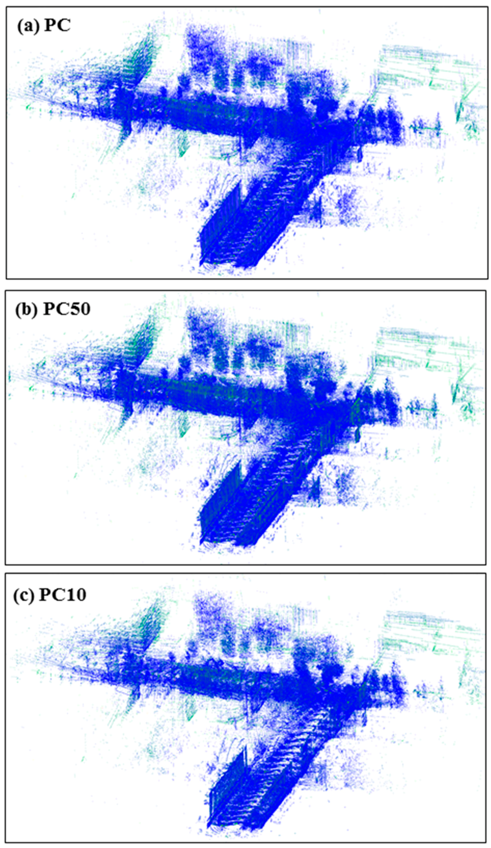
Figure 9 shows the results on a georeferenced 3D point cloud (PC).
In Figure 9b, it can be seen that, at the 50% reduction level, the point cloud does not appear in comparison to the original PC. The differences can only be noticed at the 10% reduction level, as seen in Figure 9c.
The quantitative comparison between the original and reduced point clouds are seen in Table 3.
The obtained results show how the SD values changed during the MLS dataset reduction. Even for a dataset containing only 10% of the points of the original 3D point cloud, the SD only doubled in comparison to the original SD.
Computation times were 72 s and 121 s for a 50% and 10% reduction, respectively. The data reduction for the georeferenced 3D point cloud using the OptD-single-MLS method was also very fast. It was considerably faster than the total time needed for data preparation.
5. Discussion and Conclusions
The methodology of the development of MLS measurement results consists of the following stages:
- Stage 1:
- obtaining a point cloud,
- Stage 2:
- pre-processing (including the filtration process),
- Stage 3:
- main processing (including DTM or DEM construction),
- Stage 4:
- visualization.
The modified methodology for processing large MLS datasets in stage 2 includes a reduction based on the OptD-single-MLS method. The new method allows for a fast, comprehensive, fully automated optimization in a very short time and enables the following:
- Reduction of large MLS datasets.
- Selection of the optimal dataset based on the given optimization criterion.
- Reduced main processing time (the fewer points in the dataset, the shorter the DTM or DEM generation process).
- Reduced time and costs of MLS cloud processing, which, in turn, enable effective analysis of the acquired information resources.
- Control over the size of the resulting dataset.
In this study, the authors propose a new method for the reduction of a large amount of points in a MLS dataset.
In this paper, the effect of the OptD-single-MLS method was tested in two options: (1) for MLS data taken directly from the measurement (Frame 1 and Frame 2); (2) for a georeferenced 3D point cloud.
Studies have shown that the reduction can take place either on the stopped Frame, obtained directly from the Velodyne LiDAR measurement, or can be performed on the entire 3D point cloud. The choice of options in step 1 in OptD-single-MLS depends on the purpose of the development. If we want to analyze a particular Frame from the measurement, we will select option 1; if we want to use the reduced dataset to build the DTM, then we choose option 2.
The OptD-single-MLS method provides total control over the number of points in the dataset.
Author Contributions
W.B.-B.: the concept of the article, preparation of initial assumptions, implementation of the OptD-single-MLS method, processing by the OptD-single-MLS method, preparing the figures. Z.K.: preparation of a georeferenced 3D point cloud, preparation of conclusions. C.T.: data acquisition, pre-processing of MLS data.
Funding
This research received no external funding.
Conflicts of Interest
The authors declare no conflicts of interest.
References
- Kukko, A. Road Environment Mapper—3D Data Capturing with Mobile Mapping. Licentiate’s Thesis, Helsinki University of Technology, Espoo, Finland, 2009; p. 158. [Google Scholar]
- Kukko, A.; Kaartinen, H.; Hyyppä, J.; Chen, Y. Multiplatform Mobile laser scanning: Usability and performance. Sensors 2012, 12, 11712–11733. [Google Scholar] [CrossRef]
- Szulwic, J.; Tysiąc, P. Mobile Laser Scanning Calibration on a Marine Platform. Polish Marit. Res. 2018, 25, 159–165. [Google Scholar] [CrossRef]
- Graham, L. Mobile mapping systems overview. Photogramm. Eng. Remote Sens. 2010, 76, 222–228. [Google Scholar]
- El-Halawany, S.; Moussa, A.; Lichti, D.D.; El-Sheimy, N. Detection of Road Curb from Mobile Terrestrial Laser Scanner Point Cloud. In Proceedings of the 2011 ISPRS Workshop om Laser Scanning, Calgary, AB, Canada, 29–31 August 2011. [Google Scholar]
- Hruza, P.; Mikita, T.; Tyagur, N.; Krejza, Z.; Cibulka, M.; Procházková, A.; Patočka, Z. Detecting Forest Road Wearing Course Damage Using Different Methods of Remote Sensing. Remote Sens. 2018, 10, 492. [Google Scholar] [CrossRef]
- Mikrut, S.; Kohut, P.; Pyka, K.; Tokarczyk, R.; Barszcz, T.; Uhl, T. Mobile Laser Scanning Systems for Measuring the Clearance Gauge of Railways: State of Play, Testing and Outlook. Sensors 2016, 16, 683. [Google Scholar] [CrossRef] [PubMed]
- Barber, D.; Mills, J.; Smith-Voysey, S. Geometric validation of a ground-based mobile laser scanning system. ISPRS J. Photogramm. Remote Sens. 2008, 63, 128–141. [Google Scholar] [CrossRef]
- Yen, K.S.; Akin, K.; Lofton, A.; Ravani, B.; Lasky, T.A. Using Mobile Laser Scanning to Produce Digital Terrain Models of Pavement Surfaces; Final Report of the Advanced Highway Maintenance and Construction Technology Research Center Research Project; University of California at Davies: Pittsburgh, PA, USA, 2010; Available online: http://ahmct.ucdavis.edu/pdf/UCD-ARR-10-11-30-01.pdf (accessed on 9 July 2018).
- Glennie, C.; Lichti, D.D. Static calibration and analysis of the Velodyne HDL-64E S2 for high accuracy mobile scanning. Remote Sens. 2010, 2, 1610–1624. [Google Scholar] [CrossRef]
- Suchocki, C.; Katzer, J.; Rapiński, J. Terrestrial Laser Scanner as a Tool for Assessment of Saturation and Moisture Movement in Building Materials. Periodica Polytech. Civ. Eng. 2018, 1–6. [Google Scholar] [CrossRef]
- Błaszczak-Bąk, W.; Sobieraj, A.; Janicka, J. Zastosowanie lotniczego skaningu laserowego do oceny stanu dróg w planowaniu transport. Logistyka 2015, 4, 2478–2486. [Google Scholar]
- Borkowski, A.; Keller, W. An Attempt to ALS-data filtering in wavelet domain. In Proceedings of the 8th Bilateral Geodetic Meeting Poland-Italy, Wrocław, Poland, 22–24 June 2006. [Google Scholar]
- Brenner, C. Extraction of features from mobile laser scanning data for future driver assistance systems. In Advances in GIScience; Springer: Berlin/Heidelberg, Germany, 2009. [Google Scholar]
- Bauer-Marschallinger, B.; Sabel, D.; Wagner, W. Optimisation of global grids for high-resolution remote sensing data. Comput. Geosci. 2014, 72, 84–93. [Google Scholar] [CrossRef]
- Kozioł, K.; Knecht, J.; Szombra, S. The importance of hierarchy in the generalisation of DTM. Geomat. Eng. 2012, 2, 60–75. [Google Scholar]
- Błaszczak-Bąk, W. New Optimum Dataset method in LiDAR processing. Acta Geodyn. Geomater. 2016, 13, 379–386. [Google Scholar] [CrossRef]
- Błaszczak-Bąk, W.; Sobieraj-Żłobińska, A.; Kowalik, M. The OptD-multi method in LiDAR processing. Meas. Sci. Technol. 2017, 28, 075009. [Google Scholar] [CrossRef]
- Błaszczak-Bąk, W.; Sobieraj-Żłobińska, A.; Wieczorek, B. The Optimum Dataset method—Examples of the application. E3S Web Conf. 2018, 26, 00005. [Google Scholar] [CrossRef]
- Visvalingam, M.; Whyatt, J.D. Line generalization by repeated elimination of point. Cartogr. J. 1993, 30, 46–51. [Google Scholar] [CrossRef]
- Douglas, D.H.; Peucker, T.K. Algorithms for the reduction of the number of points required to represent a digitized line or its caricature. Can. Cartogr. 1973, 10, 112–122. [Google Scholar] [CrossRef]
- Jozkow, G.; Toth, C.; Grejner-Brzezinska, D. Uas Topographic Mapping with Velodyne Lidar Sensor. ISPRS Ann. Photogramm. Remote Sens. Spat. Inf. Sci. 2016, III-1, 201–208. [Google Scholar] [CrossRef]
Figure 1.
The scheme of Options in step 1 of OptD-single-MLS.

Figure 2.
Illustration of measurement strip.

Figure 3.
D-P method on a measurement strip, (a) original; (b) after reduction with tolerance t1; (c) after reduction with tolerance t2.
Figure 3.
D-P method on a measurement strip, (a) original; (b) after reduction with tolerance t1; (c) after reduction with tolerance t2.

Figure 4.
Vehicle with measuring equipment, with Velodyne HDL-32 LiDAR.

Figure 5.
Rear view of the platform equipped with Velodyne VLP-16 LiDAR scanner.

Figure 6.
View of GPS position of vehicle.

Figure 7.
MLS data (a) original Frame 1; (b) 90% of points after reduction; (c) 80% of points after reduction; (d) 70% of points after reduction; (e) 60% of points after reduction; (f) 50% of points after reduction; (g) 40% of points after reduction; (h) 30% of points after reduction; (i) 20% of points after reduction; (j) 10% of points after reduction.

Figure 8.
MLS data (a) original Frame 2; (b) 90% of points after reduction; (c) 80% of points after reduction; (d) 70% of points after reduction; (e) 60% of points after reduction; (f) 50% of points after reduction; (g) 40% of points after reduction; (h) 30% of points after reduction; (i) 20% of points after reduction; (j) 10% of points after reduction.

Figure 9.
3D point cloud (a) original; (b) 50% of points in PC after reduction; (c) 10% of points in PC after reduction.
Figure 9.
3D point cloud (a) original; (b) 50% of points in PC after reduction; (c) 10% of points in PC after reduction.

Figure 10.
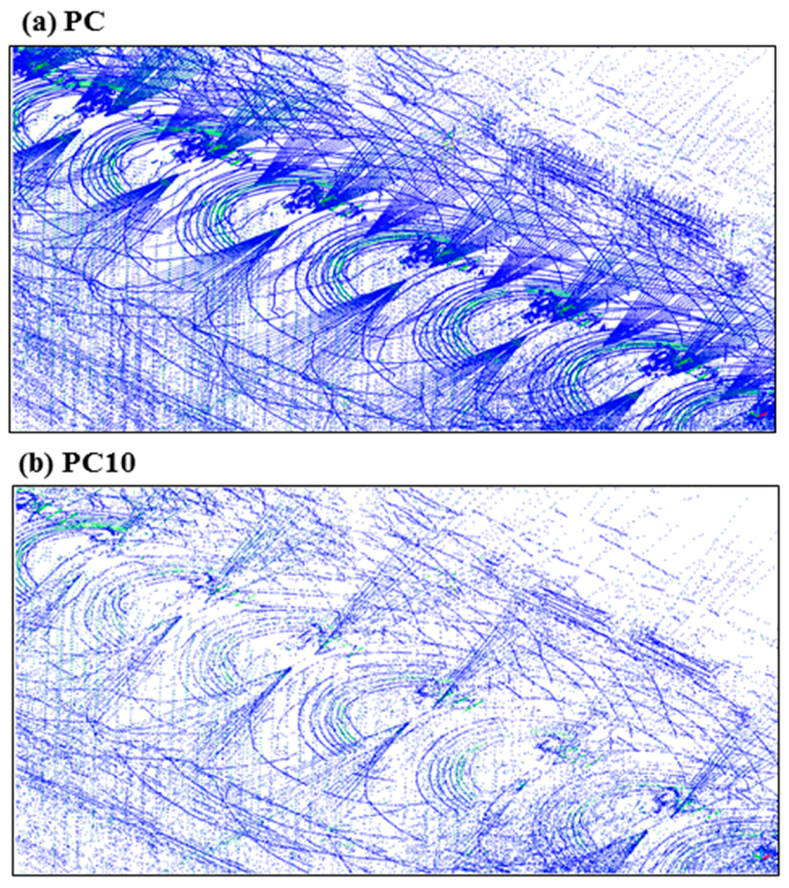
Example 1 of 3D point cloud: (a) original; (b) point cloud at 10% reduction level.

Figure 11.
Example 2 of 3D point cloud: (a) original; (b) point cloud at 10% reduction level.


Table 1.
Characteristics of obtained datasets after the OptD-single-MLS method for Frame 1.
| Parameters | |||||||
|---|---|---|---|---|---|---|---|
| Dataset | Number of Points | SD (m) | Processing Time (s) | ||||
| Frame 1 | −2.399 | 7.628 | −1.009 | 34 716 | 1.286 | - | - |
| R90 | −2.399 | 7.628 | −0.995 | 31 385 | 1.279 | −0.007 | 10 |
| R80 | −2.399 | 7.628 | −0.966 | 27 609 | 1.316 | −0.030 | 15 |
| R70 | −2.399 | 7.628 | −0.957 | 24 393 | 1.361 | −0.075 | 19 |
| R60 | −2.399 | 7.628 | −0.897 | 20 850 | 1.410 | −0.124 | 21 |
| R50 | −2.399 | 7.628 | −0.837 | 17 388 | 1.459 | −0.173 | 25 |
| R40 | −2.399 | 7.628 | −0.766 | 13 839 | 1.522 | −0.236 | 29 |
| R30 | −2.399 | 7.628 | −0.747 | 10 404 | 1.604 | −0.318 | 32 |
| R20 | −2.399 | 7.628 | −0.625 | 6 928 | 1.709 | −0.423 | 35 |
| R10 | −2.399 | 7.628 | −0.485 | 3 429 | 1.923 | −0.637 | 38 |
Table 2.
Characteristics of obtained datasets after the OptD-single-MLS method for Frame 2.
| Parameters | |||||||
|---|---|---|---|---|---|---|---|
| Dataset | Number of Points | SD (m) | Processing Time (s) | ||||
| Frame 2 | −2.402 | 7.668 | −1.018 | 34 650 | 1.283 | - | - |
| R90 | −2.402 | 7.668 | −1.004 | 31 204 | 1.281 | −0.002 | 9 |
| R80 | −2.402 | 7.668 | −0.978 | 27 975 | 1.312 | −0.029 | 15 |
| R70 | −2.402 | 7.668 | −0.967 | 24 068 | 1.362 | −0.079 | 18 |
| R60 | −2.402 | 7.668 | −0.906 | 20 831 | 1.404 | −0.121 | 20 |
| R50 | −2.402 | 7.668 | −0.846 | 17 287 | 1.450 | −0.167 | 24 |
| R40 | −2.402 | 7.668 | −0.787 | 13 867 | 1.505 | −0.222 | 29 |
| R30 | −2.402 | 7.668 | −0.766 | 10 479 | 1.570 | −0.287 | 31 |
| R20 | −2.402 | 7.668 | −0.636 | 6 863 | 1.678 | −0.395 | 37 |
| R10 | −2.402 | 7.668 | −0.491 | 3 474 | 1.929 | −0.646 | 39 |
Table 3.
Characteristics of obtained datasets after the OptD-single-MLS method for 3D PC.
| Parameters | ||||||||
|---|---|---|---|---|---|---|---|---|
| Dataset | File Size (kB) | Number of Points | SD (m) | Processing Time (s) | ||||
| PC | 682,344 | −71.562 | 87.530 | 1.165 | 19,942,752 | 2.638 | - | - |
| PC50 | 443,103 | −71.562 | 87.530 | 1.045 | 9,971,376 | 3.386 | −0.748 | 72 |
| PC10 | 70,403 | −71.562 | 87.530 | 1.032 | 1,998,727 | 5.200 | −2.562 | 121 |
© 2018 by the authors. Licensee MDPI, Basel, Switzerland. This article is an open access article distributed under the terms and conditions of the Creative Commons Attribution (CC BY) license (http://creativecommons.org/licenses/by/4.0/).
Share and Cite
MDPI and ACS Style
Błaszczak-Bąk, W.; Koppanyi, Z.; Toth, C. Reduction Method for Mobile Laser Scanning Data. ISPRS Int. J. Geo-Inf. 2018, 7, 285. https://doi.org/10.3390/ijgi7070285
AMA Style
Błaszczak-Bąk W, Koppanyi Z, Toth C. Reduction Method for Mobile Laser Scanning Data. ISPRS International Journal of Geo-Information. 2018; 7(7):285. https://doi.org/10.3390/ijgi7070285
Chicago/Turabian StyleBłaszczak-Bąk, Wioleta, Zoltan Koppanyi, and Charles Toth. 2018. "Reduction Method for Mobile Laser Scanning Data" ISPRS International Journal of Geo-Information 7, no. 7: 285. https://doi.org/10.3390/ijgi7070285
Note that from the first issue of 2016, this journal uses article numbers instead of page numbers. See further details here.