Water Level Reconstruction Based on Satellite Gravimetry in the Yangtze River Basin


1
School of Geodesy and Geomatics, Wuhan University, Wuhan 430079, China
2
Key Laboratory of Geospace Environment and Geodesy, Ministry of Education, Wuhan University, Wuhan 430079, China
*
Authors to whom correspondence should be addressed.
ISPRS Int. J. Geo-Inf. 2018, 7(7), 286; https://doi.org/10.3390/ijgi7070286
Submission received: 22 June 2018
/
Revised: 17 July 2018
/
Accepted: 19 July 2018
/
Published: 23 July 2018
Abstract
:The monitoring of hydrological extremes requires water level measurement. Owing to the decreasing number of continuous operating hydrological stations globally, remote sensing indices have been advocated for water level reconstruction recently. Nevertheless, the feasibility of gravimetrically derived terrestrial water storage (TWS) and its corresponding index for water level reconstruction have not been investigated. This paper aims to construct a correlative relationship between observed water level and basin-averaged Gravity Recovery and Climate Experiment (GRACE) TWS and its Drought Severity Index (GRACE-DSI), for the Yangtze river basin on a monthly temporal scale. The results are subsequently compared against traditional remote sensing, Palmer’s Drought Severity Index (PDSI), and El Niño Southern Oscillation (ENSO) indices. Comparison of the water level reconstructed from GRACE TWS and its index, and that of remote sensing against observed water level reveals a Pearson Correlation Coefficient (PCC) above 0.90 and below 0.84, with a Root-Mean-Squares Error (RMSE) of 0.88–1.46 m, and 1.41–1.88 m and a Nash-Sutcliffe model efficiency coefficient (NSE) above 0.81 and below 0.70, respectively. The ENSO-reconstructed water levels are comparable to those based on remote sensing, whereas the PDSI-reconstructed water level shows a similar performance to that of GRACE TWS. The water level predicted at the location of another station also exhibits a similar performance. It is anticipated that the basin-averaged, remotely-sensed hydrological variables and their standardized forms (e.g., GRACE TWS and GRACE-DSI) are viable alternatives for reconstructing water levels for large river basins affected by the hydrological extremes under ENSO influence.
1. Introduction
Lakes, reservoirs, rivers, and wetlands are regions sensitive to changing climate. Given the unstable fresh water supply due to changing climate, water level and/or volume monitoring has become an important task [1]. The water level (or stage) (WL) is a basic hydrological variable observed traditionally for a river basin. This variable is useful for monitoring the water cycle and its extremes, including floods and droughts, with a view to achieving a stable water supply [2], and paving a pathway for human sustainability in the near future [3]. Hence, continuous WL time series are necessary [4].
However, owing to a lack of maintenance funding for ground-based hydrological stations, the number of continuous operating hydrological stations has declined recently around the world [5]. An alternative for indirect WL time series measurements is desired. Hence, despite poor temporal sampling rates compared with that in ground-based measurements, remote sensing measurements have been promoted for their near-global coverage, relatively low cost, and easy accessibility [6]. Moreover, measurements can be taken at multiple virtual stations for different river sections, which is not possible with local measurements at scattered locations along a river [7].
Remotely sensed data from passive products, such as Moderate Resolution Imaging Spectrometer (MODIS), Landsat Thematic Mapper (TM), and Enhanced TM Plus (ETM+) images and active products such as satellite altimetry, have been explored since the 1990s for WL monitoring (e.g., [8]), especially for sparsely gauged remote regions [9,10]. Water surface area, floodplain inundation area, and the Normalized Difference Vegetation Index (NDVI), are commonly derived from passive remote sensing data to correlate WL or discharge including runoff because the derived data have been shown to have a good correlative relationship (e.g., [11,12,13,14,15]). However, these data are merely indicators within the hydrological cycle but are not the water balance components. Satellite radar altimetry, initially designed for sea level and ocean tidal variation studies (e.g., [16,17]), is an active remote sensing technique that can directly yield WL variations of continental surface water [18], such as lakes and rivers (e.g., [19,20,21,22,23]). However, because the radar altimetry footprint signal is contaminated by land surface (e.g., [24]), its accuracy is limited by the size of the radar altimeter footprint (i.e., 5 km for TOPEX satellite, 20 km for ERS-2 satellite, 3.4 km for Envisat satellite [25]), which is normally larger than the width of a river channel (e.g., [26]). In addition, the temporal sampling rate for the active remote sensing is normally larger than a 10-day period.
Aiming at observing monthly time-variable gravity from space, the Gravity Recovery and Climate Experiment (GRACE) mission, launched in 2002 [27], is another active remote sensing technique. It is widely used to infer large-scale terrestrial water storage (TWS) variations at a monthly temporal scale (e.g., [28,29]) and to complement the lack of large-scale TWS data from ground-based measurements [30], in which TWS is one of the components of water balance within a hydrological cycle [31]. GRACE can detect hydrological extremes (e.g., [32]) as well as groundwater depletion (e.g., [33,34]). Given the water balance formulation (i.e., ΔS = P − ET − Q) (e.g., [35]), the gravimetric-derived TWS (S) and its change (ΔS) are useful for inferring precipitation (P) [36], evapotranspiration (ET) (e.g., [37]), and runoff (Q) (e.g., [38,39,40]) for river basins, where these components except discharge can be indirectly captured by the remotely sensed data.
Han et al. (2009) [41] inferred from the GRACE inter-satellite distance change that the TWS is useful to capture basin-dependent, seasonally changing surface water, which in turn can quantitatively relate the TWS to WL variations (e.g., [42,43]). Moreover, the WL is a power function of Q that represents the runoff of the whole basin at the river mouth, called a rating curve (e.g., [31,44]), and Q is a power function of S (e.g., [45,46]). Given the abovementioned reasons, as well as the basin-wide TWS component indirectly obtained from GRACE, it is expected that WL variations at the outlet of the river basin can be captured by GRACE TWS.
In addition, several hydrological indices, such as Palmer’s Drought Severity Index (PDSI) [47] and the newly developed GRACE Drought Severity Index (GRACE-DSI) [48,49] as well as El Niño Southern Oscillation (ENSO), enable WL reconstruction [50]. This is because ENSO is an event governing the precipitation pattern (e.g., [51,52,53,54]), which affects evaporation (or evapotranspiration) and TWS [55], and, subsequently, the WL or discharge [56,57,58,59,60]. Several studies have revealed that ENSO events have an apparent teleconnection with floods and droughts (e.g., [61]), which influences the water balance components for the past, the present (e.g., [62]), and the future (e.g., [63]), in the Yangtze River Basin (YRB). These hydroclimatic characteristics make the YRB a good geographical setting for an experiment. It is anticipated that the GRACE TWS and the aforementioned indices are presumably better at capturing the variations of WL than the NDVI and land surface temperature (LST) from passive remote sensing, because these localized instantaneous responses are not the direct cause but the consequences of precipitation and water storage of a region within a hydrological cycle.
This study investigates the potential usage of the GRACE TWS and its index in reconstructing the WL time series of one hydrological station at a monthly temporal scale limited by GRACE monthly temporal sampling. The reconstructed relationship is externally validated by predicting the WL time series of another location in the Yangtze River section, where a nearby in situ station is used to assess the performance. The available remotely sensed instantaneous data (i.e., NDVI [64] and LST [65]), together with the PDSI and the ENSO indices, serve as baseline predictors for comparison with the WL reconstruction and prediction in the YRB based on satellite gravimetry.
2. Geography of Yangtze River Basin and Data Usage
2.1. Geographic Environment of the YRB
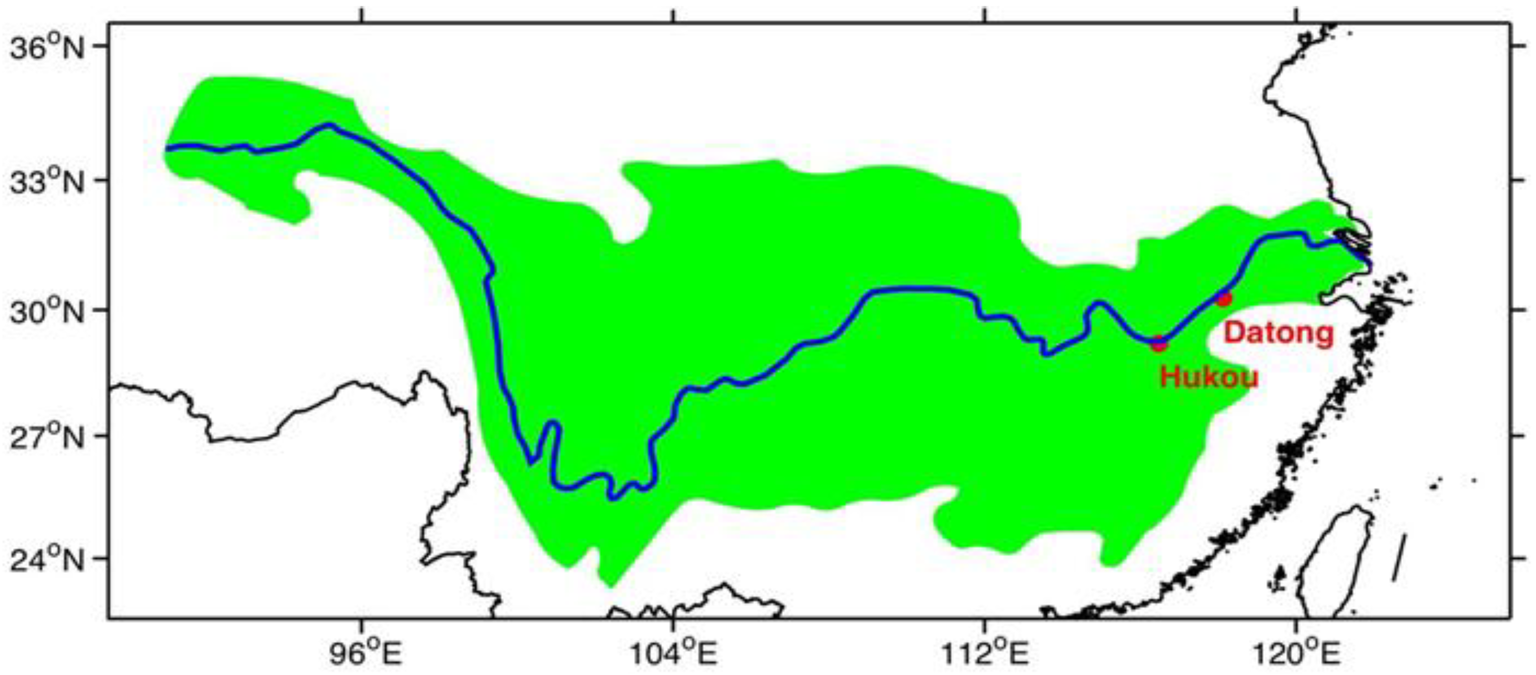
Situated at latitude 25°–35° N and longitude 91°–122° E, the YRB (Figure 1) is the longest river in China, originating from the Tibetan Plateau and flowing about 6300 km eastward into the East China Sea [66]. The basin is inhabited by 440 million people [67]. Generally, the entire YRB can be divided into three parts: the upper reach, between the Tibetan Plateau and Yichang; the middle reach between Yichang and Hukou; and the lower reach below the Hukou [68]. In addition, the YRB is affected by the subtropical monsoon climate [69].
The hydrological regime of the YRB is controlled mainly by the Indian Summer Monsoon (ISM) and the East Asian Summer Monsoon (EASM) in the Asian–Pacific system, which affects the precipitation in upper and middle–lower YRB, respectively [70]. As a result, the mean annual precipitation is 270–500 mm in the upper YRB, and 1600–1900 mm in the middle–lower YRB, respectively [71]. Under the monsoonal climate, the rainy season, ranging from April to September, generates tremendous amounts of precipitation within the YRB, particularly from mid-June to July [72].
The intensities of ISM and EASM are also affected significantly by the ENSO events [73]. In fact, significant interaction between the Asian monsoon and ENSO has been demonstrated [74,75]; the EASM over northern China and Japan can be weakened by ENSO [76]. The ISM and EASM are weakened during El Niño events, which is the warm phase of ENSO, leading to less precipitation in some regions [77]. More recently, GRACE TWS and its teleconnections to ENSO have been explored for the YRB [78] and for the globe [55]. Therefore, ENSO events have a significant influence on the hydrological variables in the YRB. This demonstrates the practicality for WL reconstruction based on GRACE TWS and ENSO information, as will be discussed in Section 4.
2.2. Ground-Based and Remote Sensing Data
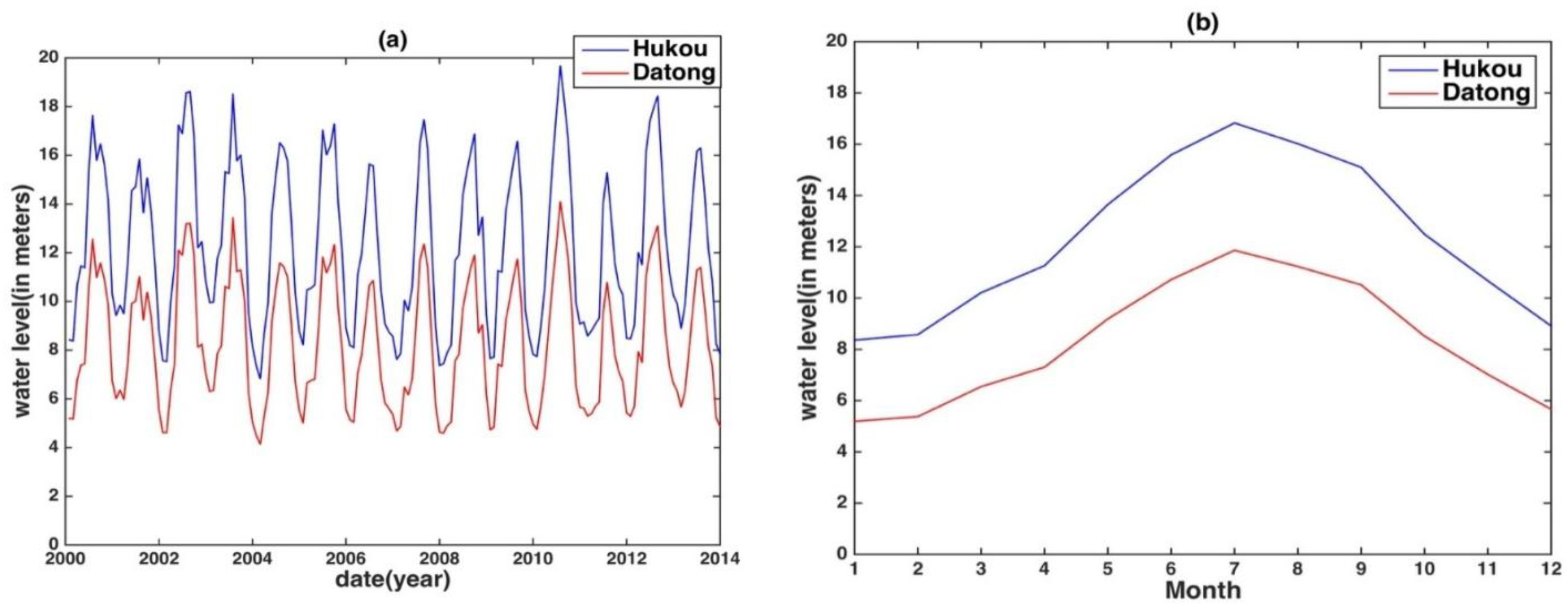
Because of the ocean tidal effect, no ground-based station has been established in close proximity to the estuary mouth of the YRB. Therefore, in situ time series data of the station closest (Datong) and the second closest station (Hukou) to the estuary mouth were chosen to reconstruct and validate the reconstructed WL, respectively, in this study (Figure 1). It should be noted that these WL data have a daily sampling rate in which the data are averaged into monthly sampling that is consistent with the remote sensing products. The time series of the two stations, with a time span between January 2000 and December 2013, were used in this study [79]. The highest and lowest WL usually occurred in July and February (Figure 2).
Remote sensing products derived from the MODIS for the land surface were used [80]. These data are available from the Land Processes Distributed Active Archive Center (LP DAAC) [81]. Within the data products, the NDVI data from the MOD13C2 product and the LST data from the MOD11C3 product were chosen as a baseline for comparison with the GRACE TWS and its index, and for the PDSI and the ENSO indices.
2.3. GRACE TWS and GRACE-DSI
GRACE time-variable gravity observations enabled us to compute monthly equivalent water height (EWH; i.e., TWS) at the global scale, with a spatial resolution of 3° (e.g., [27]). The EWH data were computed from the spherical harmonic coefficients (SHCs) of the degree-60 GRACE Level-2 Release 05 (RL05) monthly gravity field, including the calibrated uncertainties available in GeoForschungsZentrum (GFZ) [82]. The data time series spanned from January 2003 to December 2013, but the monthly data of January 2004, January 2011, June 2011, May 2012, and October 2012 were missing.
Pre-processing procedures were required to correct for geocenter motion in degree-one coefficients [83], whereas C20 term was replaced in the GRACE GSM data by the Satellite Laser Ranging (SLR) results [84] before deriving EWH. To lower the spatially correlated errors of EWH at a higher degree [85], a de-striping process [86] and Gaussian filtering with a radius of 350 km were applied [87].
The pre-processed monthly EWHs were then used to: (1) directly correlate with ground-based observed WL and (2) calculate newly proposed GRACE-DSI followed by correlating with the observed WL in a standardized form.
To avoid abnormal TWS anomalies, the median of the TWS anomalies for each month of the entire time span was used, rather than the mean of TWS anomalies proposed in Reference [48,49]. Hence, the GRACE-DSI (GI) was modified as:
where represents the TWS in year i and month j, and is the sampled standard deviation of TWS for month j separately. This standardization process can also be applied to the observed WL.
2.4. PDSI and ENSO Indices
PDSI [47] is an index that quantifies meteorological drought based on water balance within a soil moisture. It is quantified through all available temperature and rainfall data to determine the relative dryness, which ranges from −10 (dry) to +10 (wet). It has been proven to be excellent in observing secular trend of drought. These data are provided with 2.5° × 2.5° spatial resolution [88].
ENSO, a climatic event with irregular periods, is generated by the atmospheric and oceanic interaction in the tropical eastern-to-central Pacific Ocean. This event, quantifiable by sea-level atmospheric pressure differences and sea surface temperature (SST) anomalies, causes floods and droughts lasting for several months every few years or a decade [52].
Considering the different systems (i.e., ocean, atmosphere, and the coupled one) that generated the ENSO indices, we chose respectively the index SST anomalies in the tropical Pacific Ocean Niño 3.4 region, the Southern Oscillation Index (SOI), and the Multivariate ENSO Index (MEI) for this study. These data are available at [89].
3. Methodology and Assessment Scheme
3.1. Correlative Analysis and Prediction Procedures
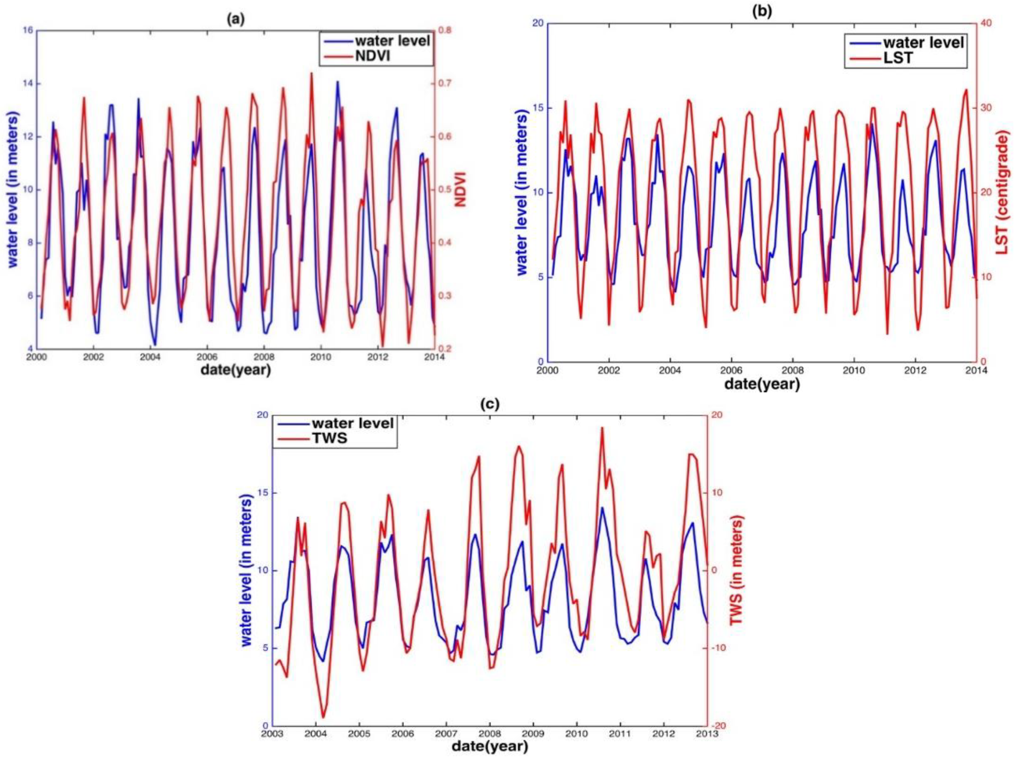
Apparent correlative relationships were revealed through a visual comparison of the observed WL time series at Datong station and the remote sensing data time series (i.e., NDVI, LST, and GRACE TWS) (Figure 3). Therefore, to establish a correlative relationship, a line fitting (i.e., an offset plus a slope) between the observed WL time series at Datong station and the remote sensing data time series (i.e., NDVI, LST, and GRACE TWS) was directly conducted within the overlapped period between January 2000 and December 2013.
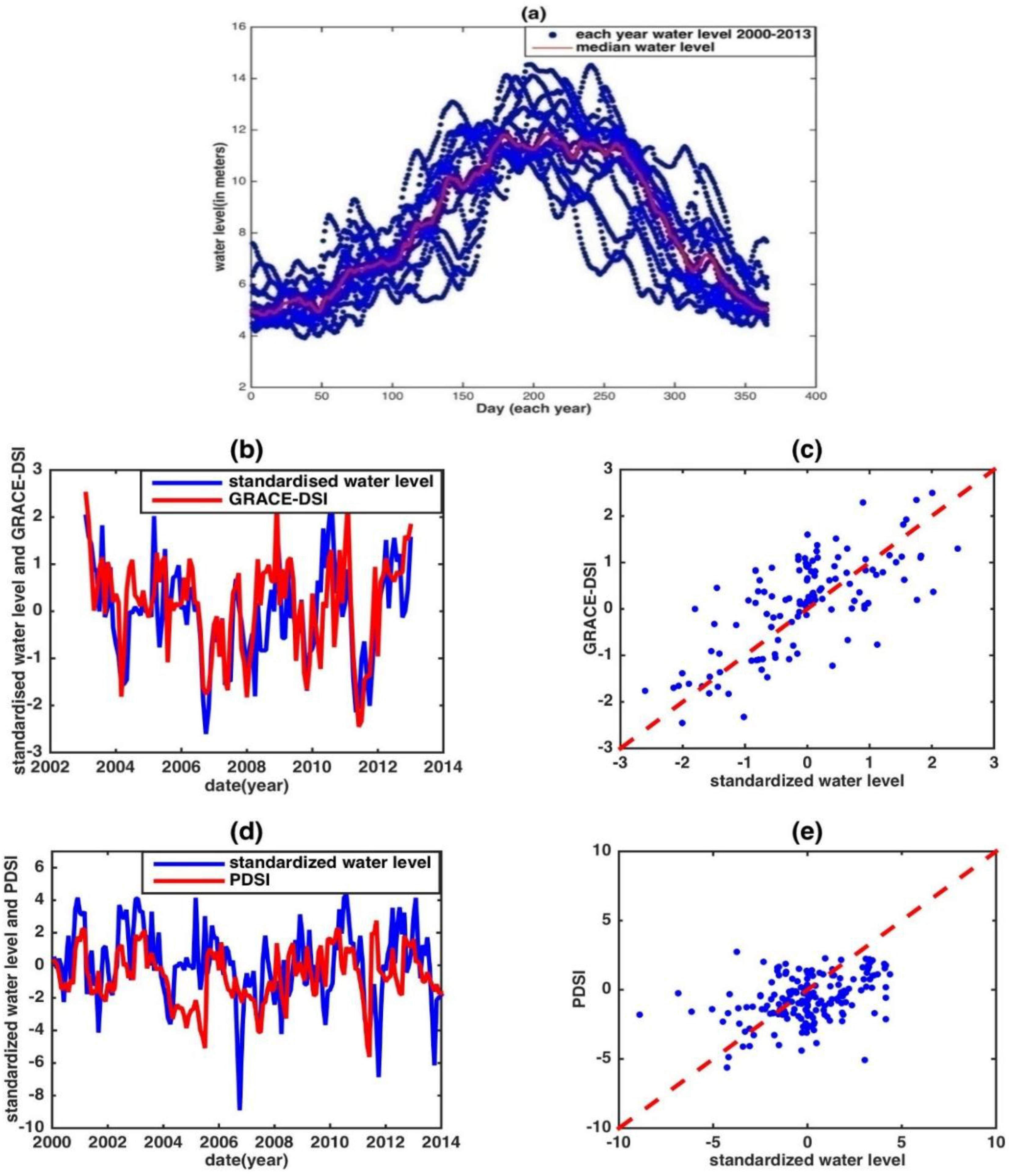
Because of the less apparent relationship between the observed WL time series and the monthly PDSI and ENSO indices, the observed WL time series were standardized using Equation (1) before establishing their relationship (Figure 4a), which is referred to as the standardized water level (SWL).
It should be noted that smoothing and re-scaling processes have been applied to the PDSI data before establishing the correlative relationship. This was achieved by obtaining the 5-month moving average of the PDSI values with re-scaling that matched the SWL. The monthly GRACE TWS and GRACE-DSI are basin-averaged time series that are comparable to the observed WL so as to minimize the local influence.
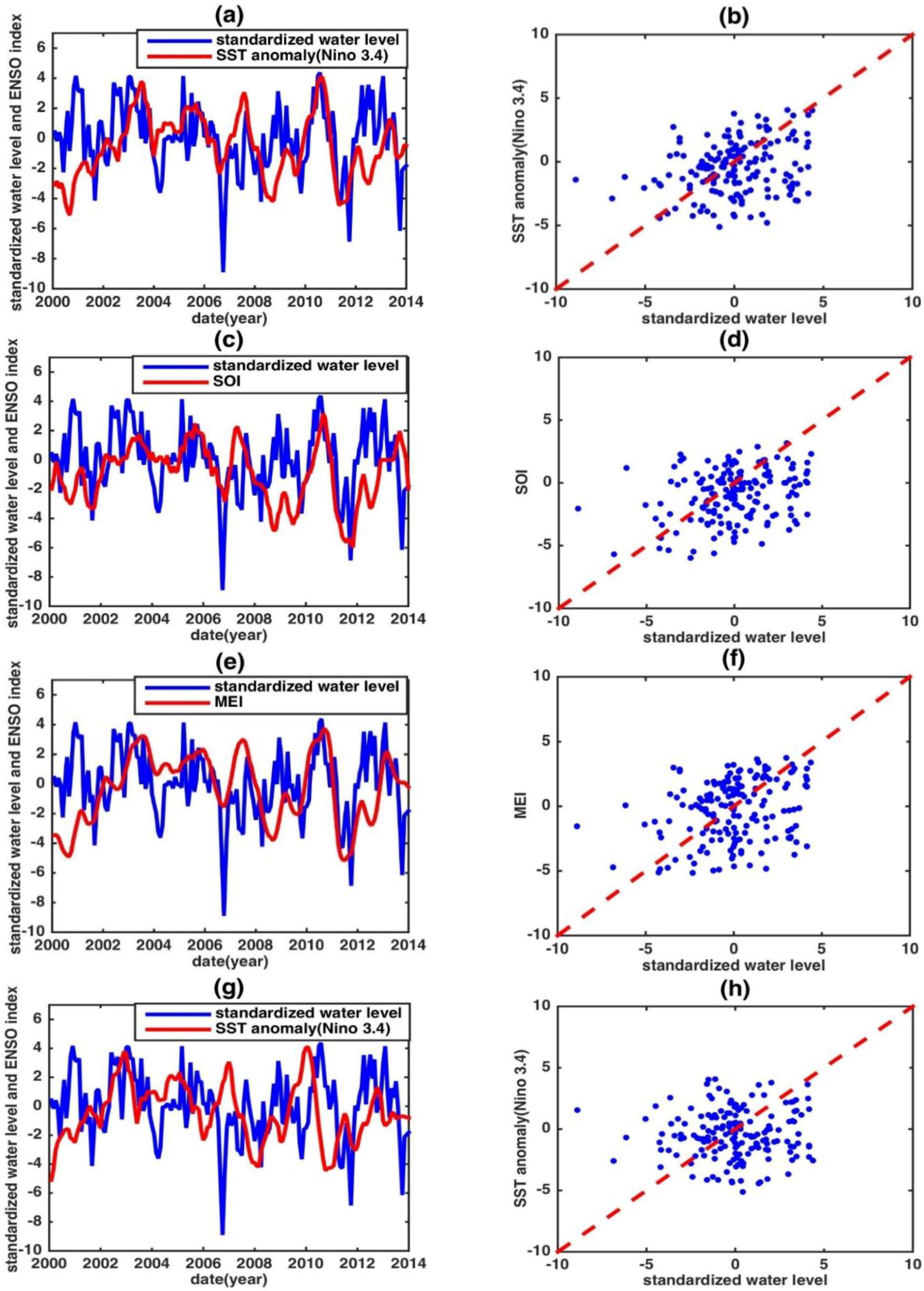
It can be observed that GRACE-DSI correlated strongly to the SWL when compared with that of PDSI (Figure 4). No apparent temporal lag between GRACE-DSI (or PDSI) and SWL was observed in the YRB. However, a 7-month temporal lag between the ENSO indices and SWL was observed (Figure 5a,g). This lag suggests teleconnection between the ENSO indices and SWL in YRB, for which hydrological modeling improvement from time lag analysis (e.g., [54]) is widely used. As a result, the 7-month temporal lag was shifted forward before the correlative relationship was established for all ENSO indices (Figure 5). After establishing the above correlative relationships, all relationships were used to reconstruct the WL time series at Datong station, and the criteria described in Section 3.2 were then internally assessed. This refers to internal assessment. Afterward, we used these relationships to predict the WL time series of another location, where the Hukou station time series were used to validate the prediction performance. This refers to external assessment.
It should be noticed that apparent offset was observed (Figure 2), which is likely attributable to height difference between two locations. Therefore, the ratio (R) owing to this height difference, obtained from the ETOPO1 1-arc-min global relief topography model [90], was applied using the below reverse procedures.
For the direct correlation relationship, the reverse formulae for the reconstructed WL () is:
where a and b are the offset and slope estimated from linear regression fitting (with an offset plus a slope) respectively, and RSD is the remote sensing data at the predicted location (i.e., NDVI and LST). An exception is that TWS is the averaged time series from upstream to the predicted location for the YRB basin.
For the correlation between the SWL and the indices, the reverse formulae is:
where and represent the reconstructed WL and the index in year i and month j, respectively.
3.2. Performance Assessment Schemes
In order to compare the observed and estimated WL time series, regardless of whether internal or external assessment was used, the Pearson Correlation Coefficient (PCC), root mean square error (RMSE), and Nash–Sutcliffe model efficiency (NSE) coefficient were selected to assess the performance. PCC is a correlative coefficient defined as:
and RMSE is an accuracy estimate given by:
The NSE [91] is a performance coefficient used to evaluate hydrological models and is calculated as:
where is the observation, is the mean of , and is the estimate. NSE ranges from −∞ to 1. NSE > 0 implies the estimate matches well with the observation, whereas NSE < 0 means the accuracy of the estimate is lower than that of the observation. NSE closest to 1 indicates the most probable estimate.
4. Results and Discussion
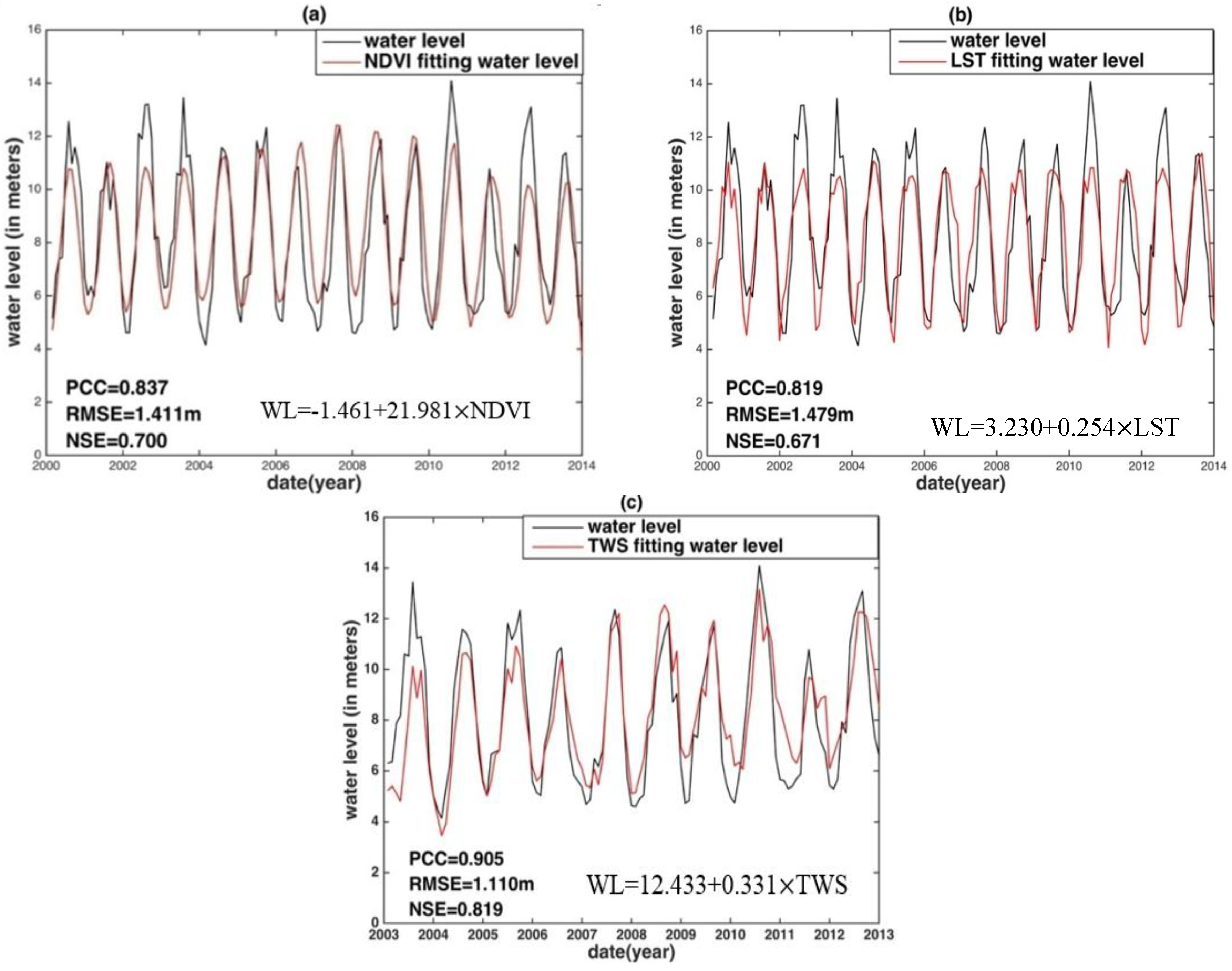
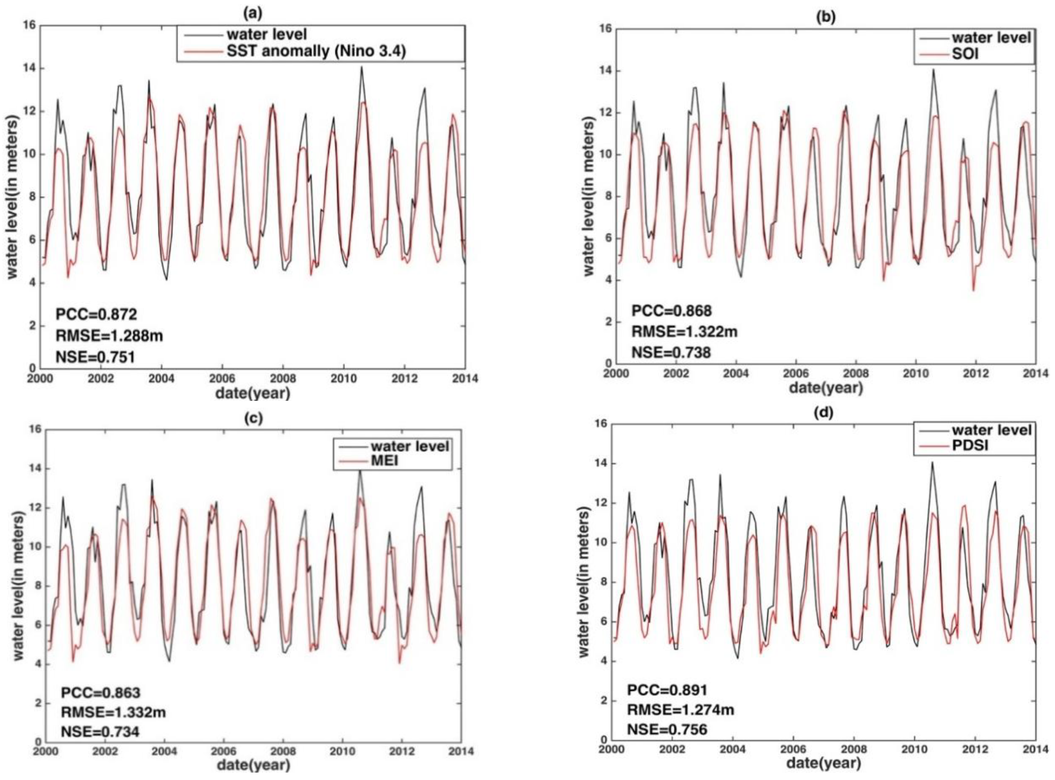
In this section, the results of the reconstructed WL time series at Datong station and the predicted time series at Hukou station are presented. Both the LST- and NDVI-reconstructed WL matched well with the observed WL (Figure 6). Nonetheless, the WL peaks between the LST-reconstructed and the observed WL displayed large disparities in 2002, 2003, 2005, 2007–2010, and 2012, with the largest one occurring in 2010. Despite the lesser magnitude, the NDVI results showed characteristics similar to that of LST and displayed large disparities in 2007 and 2010. Similar results were observed for the WL peaks between the PDSI- and ENSO-reconstructed WL and the observed WL (Figure 7).
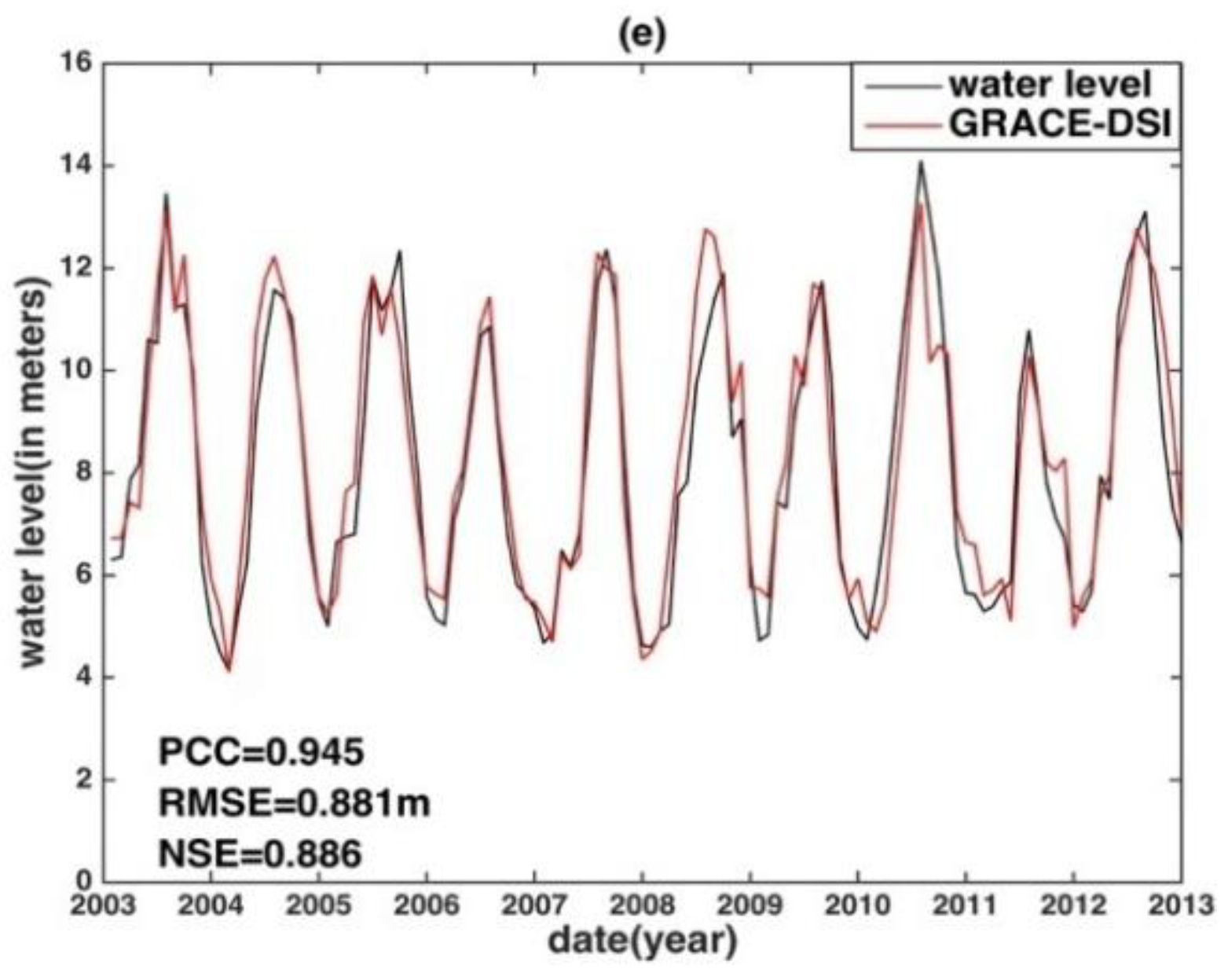
Compared with the above reconstructed WL, GRACE TWS and GRACE-DSI capture all WL peaks very well (Figure 6c and Figure 7e). GRACE-DSI displayed the best performance, regardless of whether PCC, RMSE, or NSE were used (Table 1). We speculate that TWS is a dominant water balance component within the hydrological process of the YRB and that the basin-averaged TWS is integrated information that averages out the environmental influences. GRACE-DSI displayed an even better performance, which can be attributed to its standardization process that bypasses the influence of ENSO events.
Summarizing the above result, the LST-, NDVI-, PDSI-, and ENSO-reconstructed WL are not well represented. This is because the LST and the NDVI are not water balance components that can directly relate to WL, despite their good correlation. In addition, the PDSI was made by using localized measurements that were contaminated by other environmental signals mixed with the climatic effect. Moreover, it is difficult to identify a plausible reason for the discrepancy of underestimated or overestimated ENSO-reconstructed WL peaks.
Of all reconstructed WL, GRACE TWS and GRACE-DSI perform the best, whereas all ENSO indices showed performances comparable to those of traditional remote sensing data at Datong station, as displayed in Table 1.
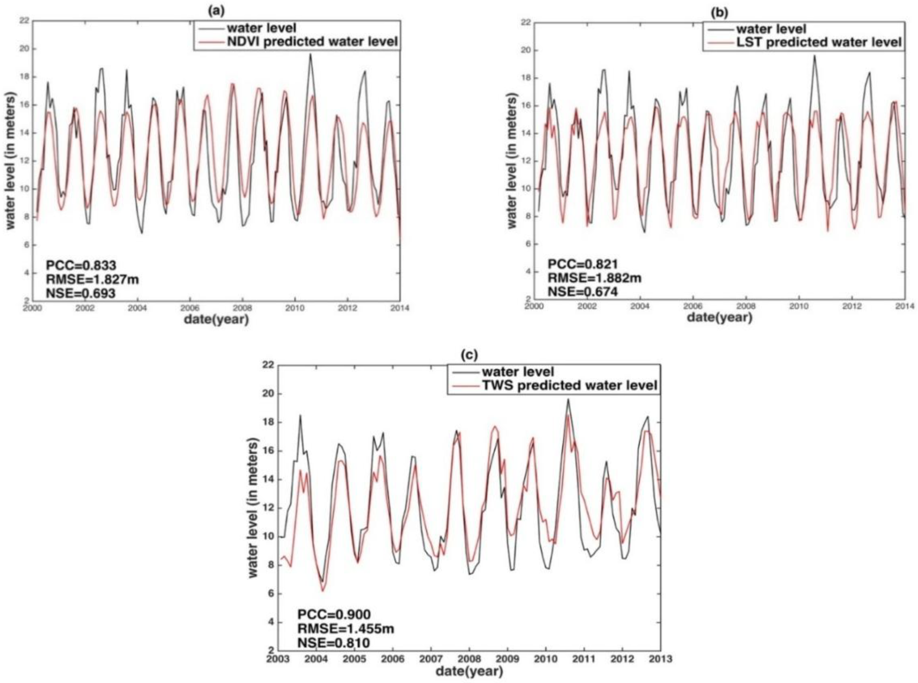
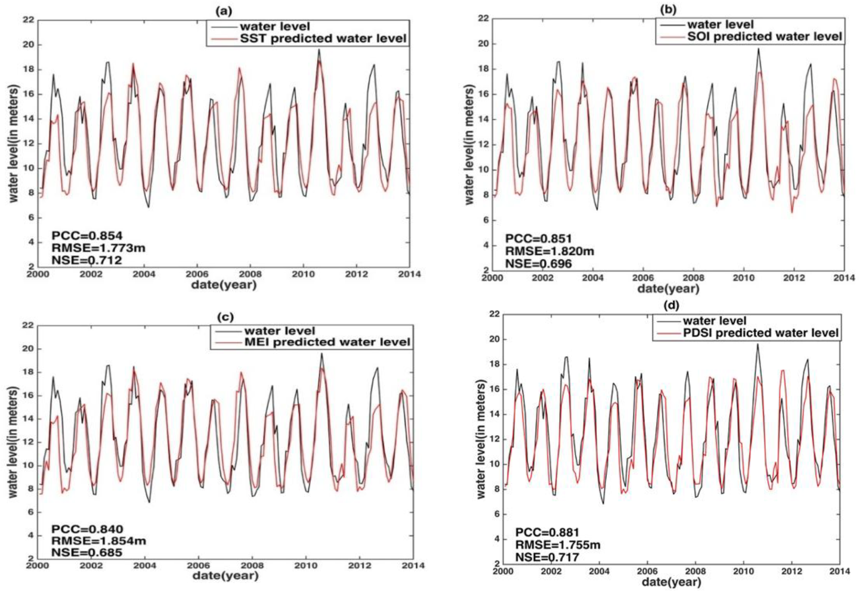
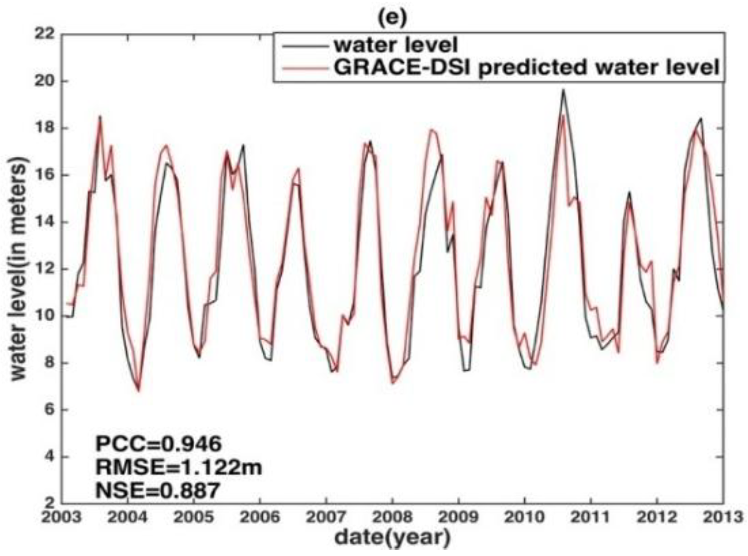
By using the reverse formula from Equations (2) and (3) in Section 3.1, the WL time series were predicted at the location of Hukou station for all data and indices used in this study (Figure 8 and Figure 9). Although the predicted Hukou WL time series were slightly less accurate than that of those recorded at Datong, Hukou WL prediction performed well (Table 1). The relative ranking of all indices also remained the same as that constructed by Datong station data.
5. Conclusions
Contrary to traditional remote sensing observations and indices (e.g., LST and NDVI), the feasibility of reconstructing the water level at one station and predicting the water level at another location for the Yangtze River Basin using GRACE TWS and its derived index (GRACE-DSI) is investigated, in addition to PDSI and three ENSO indices on a monthly temporal scale. This is because the water balance and the climatic variables and their derived indices should yield indirect causal information with the water level.
It is shown that GRACE TWS and GRACE-DSI reconstructed water levels perform better than all other indices. GRACE-DSI yields the best reconstructed water level, with a PCC of about 0.95, an RMSE value ranging from 0.88 to 1.12 m, and an NSE of about 0.89. Both GRACE TWS and PDSI show a similar performance. These results are superior to those reconstructed from traditional remote sensing with a PCC less than 0.84, RMSE ranging from 1.41 to 1.88 m, and NSE less than 0.70, whereas the ENSO-reconstructed water level shows results comparable to those of traditional remote sensing. Similar performances, in terms of their relative rankings, are obtained for the predicted water level at another station location.
It should be noted that different hydrological and climatic indices may yield different performances when projecting hydrological conditions, which depends on the drought classification (e.g., agricultural, hydrological, and meteorological), ENSO influence, and hydro-geological properties of different river basins. Yet, a more comprehensive assessment is essential to verify the presented results further, with the inclusion of environmental indices derived from climate model outputs [92] for water level projections. In addition, with the improved temporal resolution of the above indices, our methodology will be further extended to include runoff-storage hysteretic analysis, and different combinations of hydrological variables and their corresponding indices for more efficient water level reconstruction and estimation.
Author Contributions
H.S.F. designed an initial concept and experiment with data collection, performed analyses and interpretation, and wrote the manuscript. Q.H. performed data pre-processing and post-processing and contributed to the revised manuscript.
Funding
This research is partly supported by the National Natural Science Foundation of China (NSFC) (Grant No. 41674007; 41429401). The authors appreciate the historical water level data provided from Changjiang Water Resources Commission, Ministry of Water Resources (http://www.cjh.com.cn) purchased under NSFC (Grant No. 41374010), and the National Basic Research Program of China (973 Program; Grant No. 2013CB733302).
Conflicts of Interest
The authors declare no conflict of interest.
References
- Alsdorf, D.E.; Rodriguez, E.; Lettenmaier, D.P. Measuring surface water from space. Rev. Geophys. 2007, 45. [Google Scholar] [CrossRef] [Green Version]
- Jung, H.C.; Alsdorf, D.; Moritz, M.; Lee, H.; Vassolo, S. Analysis of the relationship between flooding area and water height in the Logone floodplain. Phys. Chem. Earth Parts A/B/C 2011, 36, 232–240. [Google Scholar] [CrossRef]
- Postel, S.L.; Daily, G.C.; Ehrlich, P.R. Human appropriation of renewable fresh water. Science 1996, 271, 785–788. [Google Scholar] [CrossRef]
- Vörösmarty, C.; Willmott, C.J.; Choudhury, B.J.; Schloss, A.L.; Steams, T.K.; Robeson, S.M.; Dorman, T.J. Analyzing the discharge regime of a large tropical river through remote sensing, ground-based climatic data, and modeling. Water Resour. Res. 1996, 32, 3137–3150. [Google Scholar] [CrossRef]
- Vörösmarty, C.; Askew, A.; Grabs, W.; Barry, R.; Birkett, C.; Döll, P.; Goodison, B.; Hall, A.; Jenne, R.; Kitaev, L. Global water data: A newly endangered species. Eos Trans. Am. Geophys. Union 2001, 82, 54–58. [Google Scholar] [CrossRef]
- Yan, K.; Baldassarre, G.D.; Solomatine, D.P.; Schumann, G.J.P. A review of low-cost space-borne data for flood modelling: Topography, flood extent and water level. Hydrol. Process. 2015, 29, 3368–3387. [Google Scholar] [CrossRef]
- Mersel, M.K.; Smith, L.C.; Andreadis, K.M.; Durand, M.T. Estimation of river depth from remotely sensed hydraulic relationships. Water Resour. Res. 2013, 49, 3165–3179. [Google Scholar] [CrossRef] [Green Version]
- Alsdorf, D.E.; Lettenmaier, D.P. Tracking fresh water from space. Science 2003, 301, 1491–1494. [Google Scholar] [CrossRef] [PubMed]
- Song, C.; Ye, Q.; Sheng, Y.; Gong, T. Combined ICESat and CryoSat-2 altimetry for accessing water level dynamics of Tibetan Lakes over 2003–2014. Water 2015, 7, 4685–4700. [Google Scholar] [CrossRef]
- Tang, Q.; Gao, H.; Lu, H.; Lettenmaier, D.P. Remote sensing: Hydrology. Prog. Phys. Geogr. 2009, 33, 490–509. [Google Scholar] [CrossRef]
- Smith, L.C. Satellite remote sensing of river inundation area, stage, and discharge: A review. Hydrol. Process. 1997, 11, 1427–1439. [Google Scholar] [CrossRef]
- Liu, W.T.; Juárez, R.I.N. ENSO drought onset prediction in northeast Brazil using NDVI. Int. J. Remote Sens. 2001, 22, 3483–3501. [Google Scholar] [CrossRef]
- Pan, F.; Nichols, J. Remote sensing of river stage using the cross-sectional inundation area-river stage relationship (IARSR) constructed from digital elevation model data. Hydrol. Process. 2013, 27, 3596–3606. [Google Scholar] [CrossRef]
- Li, L.; Vrieling, A.; Skidmore, A.; Wang, T.; Muñoz, A.R.; Turak, E. Evaluation of MODIS spectral indices for monitoring hydrological dynamics of a small, seasonally-flooded wetland in southern Spain. Wetlands 2015, 35, 851–864. [Google Scholar] [CrossRef]
- Shrestha, R.; Di, L.; Eugene, G.Y.; Kang, L.; Shao, Y.Z.; Bai, Y.Q. Regression model to estimate flood impact on corn yield using MODIS NDVI and USDA cropland data layer. J. Integr. Agric. 2017, 16, 398–407. [Google Scholar] [CrossRef]
- Fu, L.L.; Christensen, E.J.; Yamarone, C.A.; Lefebvre, M.; Menard, Y.; Dorrer, M.; Escudier, P. TOPEX/POSEIDON mission overview. J. Geophys. Res. 1994, 99, 24369–24381. [Google Scholar] [CrossRef]
- Fok, H.S. Ocean Tides Modeling Using Satellite Altimetry. Ph.D. Thesis, The Ohio State University, Columbus, OH, USA, 2012. [Google Scholar]
- Berry, P.A.M.; Garlick, J.D.; Freeman, J.A.; Mathers, E.L. Global inland water monitoring from multi-mission altimetry. Geophys. Res. Lett. 2005, 32, 101–120. [Google Scholar] [CrossRef]
- Kouraev, A.V.; Zakharova, E.A.; Samain, O.; Mognard, N.M.; Cazenave, A. Ob’river discharge from TOPEX/Poseidon satellite altimetry (1992–2002). Remote Sens. Environ. 2004, 93, 238–245. [Google Scholar] [CrossRef]
- Frappart, F.; Minh, K.D.; L’Hermitte, J.; Cazenave, A.; Ramillien, G.; Le Toan, T.; Mognard-Campbell, N. Water volume change in the lower Mekong from satellite altimetry and imagery data. Geophys. J. Int. 2006, 167, 570–584. [Google Scholar] [CrossRef] [Green Version]
- Calmant, S.; Seyler, F.; Cretaux, J.F. Monitoring continental surface waters by satellite altimetry. Surv. Geophys. 2008, 29, 247–269. [Google Scholar] [CrossRef]
- Birkinshaw, S.J.; O’donnell, G.M.; Moore, P.; Kilsby, C.G.; Fowler, H.J.; Berry, P.A.M. Using satellite altimetry data to augment flow estimation techniques on the Mekong River. Hydrol. Process. 2010, 24, 3811–3825. [Google Scholar] [CrossRef]
- Tarpanelli, A.; Barbetta, S.; Brocca, L.; Moramarco, T. River discharge estimation by using altimetry data and simplified flood routing modeling. Remote Sens. 2013, 5, 4145–4162. [Google Scholar] [CrossRef]
- Tseng, K.H.; Shum, C.K.; Yi, Y.; Emery, W.J.; Kuo, C.Y.; Lee, H.; Wang, H. The improved retrieval of coastal sea surface heights by retracking modified radar altimetry waveforms. IEEE Trans. Geosci. Remote Sens. 2014, 52, 991–1001. [Google Scholar] [CrossRef]
- Phan, V.H.; Lindenbergh, R.; Menenti, M. ICESat derived elevation changes of Tibetan lakes between 2003 and 2009. Int. J. Appl. Earth Obs. 2012, 17, 12–22. [Google Scholar] [CrossRef]
- Crétaux, J.F.; Abarca-del-Río, R.; Berge-Nguyen, M.; Arsen, A.; Drolon, V.; Clos, G.; Maisongrande, P. Lake volume monitoring from space. Surv. Geophys. 2016, 37, 269–305. [Google Scholar] [CrossRef]
- Tapley, B.D.; Bettadpur, S.; Watkins, M.; Reigber, C. The gravity recovery and climate experiment: Mission overview and early results. Geophys. Res. Lett. 2004, 31, L09607. [Google Scholar] [CrossRef]
- Wahr, J.; Swenson, S.; Zlotnicki, V.; Velicogna, I. Time-variable gravity from GRACE: First results. Geophys. Res. Lett. 2004, 31, L11501. [Google Scholar] [CrossRef]
- Crowley, J.W.; Mitrovica, J.X.; Bailey, R.C.; Tamisiea, M.E.; Davis, J.L. Land water storage within the Congo Basin inferred from GRACE satellite gravity data. Geophys. Res. Lett. 2006, 33, L19402. [Google Scholar] [CrossRef]
- Lettenmaier, D.P.; Famiglietti, J.S. Hydrology: Water from on high. Nature 2006, 444, 562. [Google Scholar] [CrossRef] [PubMed]
- Beven, K.J. Rainfall-Runoff Modelling: The Primer; John Wiley & Sons: Hoboken, NJ, USA, 2011. [Google Scholar]
- Chen, J.L.; Wilson, C.R.; Tapley, B.D. The 2009 exceptional Amazon flood and interannual terrestrial water storage change observed by GRACE. Water Resour. Res. 2010, 46, 439–445. [Google Scholar] [CrossRef]
- Rodell, M.; Velicogna, I.; Famiglietti, J.S. Satellite-based estimates of groundwater depletion in India. Nature 2009, 460, 999–1002. [Google Scholar] [CrossRef] [PubMed] [Green Version]
- Scanlon, B.R.; Longuevergne, L.; Long, D. Ground referencing GRACE satellite estimates of groundwater storage changes in the California Central Valley, USA. Water Resour. Res. 2012, 48, W04520. [Google Scholar] [CrossRef]
- Zhang, Y.; Pan, M.; Wood, E.F. On creating global gridded terrestrial water budget estimates from satellite remote sensing. Surv. Geophys. 2016, 37, 249–268. [Google Scholar] [CrossRef]
- Frappart, F.; Ramillien, G.; Ronchail, J. Changes in terrestrial water storage versus rainfall and discharges in the Amazon basin. Int. J. Climatol. 2013, 33, 3029–3046. [Google Scholar] [CrossRef] [Green Version]
- Rodell, M.; Famiglietti, J.S.; Chen, J.; Seneviratne, S.I.; Viterbo, P.; Holl, S.; Wilson, C.R. Basin scale estimates of evapotranspiration using GRACE and other observations. Geophys. Res. Lett. 2004, 31, 183–213. [Google Scholar] [CrossRef]
- Syed, T.H.; Famiglietti, J.S.; Chambers, D.P. GRACE-based estimates of terrestrial freshwater discharge from basin to continental scales. J. Hydrometeorol. 2009, 10, 22–40. [Google Scholar] [CrossRef]
- Ferreira, V.G.; Gong, Z.; He, X.; Zhang, Y.; Andam-Akorful, S.A. Estimating total discharge in the Yangtze River Basin using satellite-based observations. Remote Sens. 2013, 5, 3415–3430. [Google Scholar] [CrossRef]
- Sichangi, A.W.; Wang, L.; Yang, K.; Chen, D.; Wang, Z.; Li, X.; Zhou, J.; Liu, W.; Kuria, D. Estimating continental river basin discharges using multiple remote sensing data sets. Remote Sens. Environ. 2016, 179, 36–53. [Google Scholar] [CrossRef]
- Han, S.C.; Kim, H.; Yeo, I.Y.; Yeh, P.; Oki, T.; Seo, K.W.; Alsdorf, D.; Luthcke, S.B. Dynamics of surface water storage in the Amazon inferred from measurements of inter-satellite distance change. Geophys. Res. Lett. 2009, 36, 8379–8387. [Google Scholar] [CrossRef]
- Singh, A.; Seitz, F.; Schwatke, C. Inter-annual water storage changes in the Aral Sea from multi-mission satellite altimetry, optical remote sensing, and GRACE satellite gravimetry. Remote Sens. Environ. 2012, 123, 187–195. [Google Scholar] [CrossRef]
- Khan, H.H.; Khan, A.; Ahmed, S.; Gennero, M.C.; Do Minh, K.; Cazenave, A. Terrestrial water dynamics in the lower Ganges—Estimates from ENVISAT and GRACE. Arab. J. Geosci. 2013, 6, 3693–3702. [Google Scholar] [CrossRef]
- Tourian, M.J.; Sneeuw, N.; Bárdossy, A. A quantile function approach to discharge estimation from satellite altimetry (ENVISAT). Water Resour. Res. 2013, 49, 4174–4186. [Google Scholar] [CrossRef] [Green Version]
- Riegger, J.; Tourian, M.J. Characterization of runoff-storage relationships by satellite gravimetry and remote sensing. Water Resour. Res. 2014, 50, 3444–3466. [Google Scholar] [CrossRef] [Green Version]
- Sproles, E.A.; Leibowitz, S.G.; Reager, J.T.; Wigington, P.J.; Famiglietti, J.S.; Patil, S.D. GRACE storage-runoff hystereses reveal the dynamics of regional watersheds. Hydrol. Earth Syst. Sci. 2015, 19, 3253–3272. [Google Scholar] [CrossRef]
- Palmer, W.C. Meteorological Drought; Department of Commerce, Weather Bureau: Washington, DC, USA, 1965; Volume 30. [Google Scholar]
- Thomas, B.F.; Famiglietti, J.S.; Landerer, F.W.; Wiese, D.N.; Molotch, N.P.; Argus, D.F. GRACE groundwater drought index: Evaluation of California Central Valley groundwater drought. Remote Sens. Environ. 2017, 198, 384–392. [Google Scholar] [CrossRef]
- Zhao, M.; Velicogna, I.; Kimball, J.S. Satellite observations of regional drought severity in the continental United States using GRACE-based terrestrial water storage changes. J. Clim. 2017, 30, 6297–6308. [Google Scholar] [CrossRef]
- Fok, H.S.; He, Q.; Chun, K.P.; Zhou, Z.; Chu, T. Application of ENSO and Drought Indices for Water Level Reconstruction and Prediction: A Case Study in the Lower Mekong River Estuary. Water 2018, 10, 58. [Google Scholar] [CrossRef]
- Dettinger, M.D.; Diaz, H.F. Global characteristics of stream flow seasonality and variability. J. Hydrometeorol. 2000, 1, 289–310. [Google Scholar] [CrossRef]
- Kiem, A.S.; Franks, S.W. On the identification of ENSO-induced rainfall and runoff variability: A comparison of methods and indices. Hydrol. Sci. J. 2001, 46, 715–727. [Google Scholar] [CrossRef]
- Sheffield, J.; Wood, E.F. Global trends and variability in soil moisture and drought characteristics, 1950–2000, from observation-driven simulations of the terrestrial hydrologic cycle. J. Clim. 2008, 21, 432–458. [Google Scholar] [CrossRef]
- Yao, S.; Huang, Q.; Zhao, C. Variation Characteristics of Rainfall in the Pre-Flood Season of South China and Its Correlation with Sea Surface Temperature of Pacific. Atmosphere 2015, 7, 5. [Google Scholar] [CrossRef]
- Ni, S.; Chen, J.; Wilson, C.R.; Li, J.; Hu, X.; Fu, R. Global Terrestrial Water Storage Changes and Connections to ENSO Events. Surv. Geophys. 2018, 39, 1–22. [Google Scholar] [CrossRef]
- Räsänen, T.A.; Kummu, M. Spatiotemporal influences of ENSO on precipitation and flood pulse in the Mekong River Basin. J. Hydrol. 2013, 476, 154–168. [Google Scholar] [CrossRef]
- Kiem, A.S.; Hapuarachchi, H.P.; Ishidaira, H.; Magome, J.; Takeuchi, K. Uncertainty in hydrological predictions due to inadequate representation of climate variability impacts. In Proceedings of the AOGS 1st Annual Meeting & APHW 2nd Conference, Singapore, 5–9 July 2004. [Google Scholar]
- Xue, Z.; Liu, J.P.; Ge, Q. Changes in hydrology and sediment delivery of the Mekong River in the last 50 years: Connection to damming, monsoon, and ENSO. Earth Surf. Process. Landf. 2011, 36, 296–308. [Google Scholar] [CrossRef]
- Wooldridge, S.A.; Franks, S.W.; Kalma, J.D. Hydrological implications of the Southern Oscillation: Variability of the rainfall-runoff relationship. Hydrol. Sci. J. 2001, 46, 73–88. [Google Scholar] [CrossRef]
- Li, S.; He, D. Water level response to hydropower development in the upper Mekong River. AMBIO J. Hum. Environ. 2008, 37, 170–176. [Google Scholar] [CrossRef]
- Tong, J.; Qiang, Z.; Deming, Z.; Yijin, W. Yangtze floods and droughts (China) and teleconnections with ENSO activities (1470–2003). Quat. Int. 2006, 144, 29–37. [Google Scholar] [CrossRef]
- Wei, W.; Chang, Y.; Dai, Z. Streamflow changes of the Changjiang (Yangtze) River in the recent 60 years: Impacts of the East Asian summer monsoon, ENSO, and human activities. Quat. Int. 2014, 336, 98–107. [Google Scholar] [CrossRef]
- Xu, Y.; Xu, C.; Gao, X.; Luo, Y. Projected changes in temperature and precipitation extremes over the Yangtze River Basin of China in the 21st century. Quat. Int. 2009, 208, 44–52. [Google Scholar] [CrossRef]
- Tucker, C.J. Red and photographic infrared linear combinations for monitoring vegetation. Remote Sens. Environ. 1979, 8, 127–150. [Google Scholar] [CrossRef] [Green Version]
- Forsythe, N.; Kilsby, C.G.; Fowler, H.J.; Archer, D.R. Assessment of runoff sensitivity in the Upper Indus Basin to interannual climate variability and potential change using MODIS satellite data products. Mt. Res. Dev. 2012, 32, 16–29. [Google Scholar] [CrossRef]
- Zhang, Q.; Jiang, T.; Gemmer, M.; Becker, S. Precipitation, temperature and runoff analysis from 1950 to 2002 in the Yangtze basin, China. Hydrol. Sci. J. 2005, 50, 65–80. [Google Scholar]
- Sang, Y.F.; Wang, Z.G.; Liu, C.M. Spatial and temporal variability of daily temperature during 1961–2010 in the Yangtze River Basin, China. Quat. Int. 2012, 304, 33–42. [Google Scholar] [CrossRef]
- Chen, Z.; Li, J.; Shen, H.; Wang, Z. Yangtze River of China: Historical analysis of discharge variability and sediment flux. Geomorphology 2001, 41, 77–91. [Google Scholar] [CrossRef]
- Zhao, G.J.; Hörmann, G.; Fohrer, N.; Gao, J.F.; Zhai, J.Q.; Zhang, Z.X. Spatial and temporal characteristics of wet spells in the Yangtze River Basin from 1961 to 2003. Theor. Appl. Climatol. 2009, 98, 107–117. [Google Scholar] [CrossRef]
- Ding, Y.; Chan, J.C.L. The East Asian summer monsoon: An overview. Meteorol. Atmos. Phys. 2005, 89, 117–142. [Google Scholar]
- Yu, F.; Chen, Z.; Ren, X.; Yang, G. Analysis of historical floods on the Yangtze River, China: Characteristics and explanations. Geomorphology 2009, 113, 210–216. [Google Scholar] [CrossRef]
- Chen, Z.; Zhao, Y. Impact on the Yangtze (Changjiang) estuary from its drainage basin: Sediment load and discharge. Chin. Sci. Bull. 2001, 46, 73–80. [Google Scholar] [CrossRef]
- Yasunari, T. Impact of Indian monsoon on the coupled atmosphere/ocean system in the tropical Pacific. Meteorol. Atmos. Phys. 1990, 44, 29–41. [Google Scholar] [CrossRef]
- Lau, N.-C.; Wang, B. Interactions between the Asian monsoon and the El Niño/Southern oscillation. In The Asian Monsoon; Springer: Berlin/Heidelberg, Germany, 2006; pp. 479–512. [Google Scholar]
- Wang, B.; Wu, R.; Lau, K. Interannual variability of the Asian summer monsoon: Contrasts between the Indian and the western North Pacific–East Asian monsoons. J. Clim. 2001, 14, 4073–4090. [Google Scholar] [CrossRef]
- Wu, R.; Wang, B. A contrast of the East Asian summer monsoon—ENSO relationship between 1962–77 and 1978–93. J. Clim. 2002, 15, 3266–3279. [Google Scholar] [CrossRef]
- Juneng, L.; Tangang, F.T. Evolution of ENSO-related rainfall anomalies in Southeast Asia region and its relationship with atmosphere–ocean variations in Indo-Pacific sector. Clim. Dyn. 2005, 25, 337–350. [Google Scholar] [CrossRef]
- Zhang, Z.; Chao, B.F.; Chen, J.; Wilson, C.R. Terrestrial water storage anomalies of Yangtze River Basin droughts observed by GRACE and connections with ENSO. Glob. Planet. Chang. 2015, 126, 35–45. [Google Scholar] [CrossRef]
- Yangtze (Changjiang) Water Resources Commission, Ministry of Water Resources. Available online: http://www.cjh.com.cn (accessed on 10 June 2018).
- Justice, C.O.; Vermote, E.; Townshend, J.R.; Defries, R.; Roy, D.P.; Hall, D.K.; Salomonson, V.V.; Privette, J.L.; Riggs, G.; Strahler, A. The Moderate Resolution Imaging Spectroradiometer (MODIS): Land remote sensing for global change research. IEEE Trans. Geosci. Remote Sens. 1998, 36, 1228–1249. [Google Scholar] [CrossRef]
- National Aeronautics and Space Administration (NASA) Earth Observing System Data and Information System (ESDIS) Project. Available online: https://lpdaac.usgs.gov/dataset_discovery/modis/modis_products_table (accessed on 15 June 2018).
- GeoForschungsZentrum (GFZ) GRACE Level-2 Release 05 (RL05) Monthly Gravity Field. Available online: ftp://rz-vm152.gfz-potsdam.de/grace/ (accessed on 18 May 2018).
- Swenson, S.; Chambers, D.; Wahr, J. Estimating geocenter variations from a combination of GRACE and ocean model output. J. Geophys. Res. Solid Earth 2008, 113, B8. [Google Scholar] [CrossRef]
- Cheng, M.; Tapley, B.D. Variations in the earth’s oblateness during the past 28 years. J. Geophys. Res. Solid Earth 2004, 109, B9. [Google Scholar] [CrossRef]
- Ramillien, G.; Frappart, F.; Cazenave, A.; Güntner, A. Time variations of land water storage from an inversion of 2 years of GRACE geoids. Earth Planet. Sci. Lett. 2005, 235, 283–301. [Google Scholar] [CrossRef] [Green Version]
- Chambers, D.P. Observing seasonal steric sea level variations with GRACE and satellite altimetry. J. Geophys. Res. 2006, 111, C03010. [Google Scholar] [CrossRef]
- Swenson, S.; Wahr, J. Post-processing removal of correlated errors in GRACE data. Geophys. Res. Lett. 2006. [Google Scholar] [CrossRef]
- Dai, A.; Trenberth, K.E.; Qian, T. A global dataset of Palmer Drought Severity Index for 1870–2002: Relationship with soil moisture and effects of surface warming. J. Hydrometeorol. 2004, 5, 1117–1130. [Google Scholar] [CrossRef]
- Climate Indices: Monthly Atmospheric and Ocean Time Series. Available online: https://www.esrl.noaa.gov/psd/data/climateindices/list/ (accessed on 7 June 2018).
- Amante, C.; Eakins, B.W. ETOPO1 1 Arc-Minute Global Relief Model: Procedures, Data Sources and Analysis; NOAA Technical Memorandum NGDC-24; National Geophysical Data Centre, NESDIS, NOAA, Department of Commerce: Boulder, CO, USA, 2009.
- Nash, J.E.; Sutcliffe, J.V. River flow forecasting through conceptual models part I—A discussion of principles. J. Hydrol. 1970, 10, 282–290. [Google Scholar] [CrossRef]
- Lofgren, B.M.; Rouhana, J. Physically Plausible Methods for Projecting Changes in Great Lakes Water Levels under Climate Change Scenarios. J. Hydrometeorol. 2016, 17, 2209–2223. [Google Scholar] [CrossRef]
Figure 1.
Map of the Yangtze River Basin with selected stations in red dots situated near the river mouth.
Figure 1.
Map of the Yangtze River Basin with selected stations in red dots situated near the river mouth.

Figure 2.
Monthly-averaged water level time series (a) and mean monthly-averaged water level (b) at Hukou (blue) and Datong (red) stations originating from daily water level data.
Figure 2.
Monthly-averaged water level time series (a) and mean monthly-averaged water level (b) at Hukou (blue) and Datong (red) stations originating from daily water level data.

Figure 3.
Comparison of the time series of monthly-averaged water levels recorded at Datong (blue) station and (a) NDVI; (b) LST and (c) TWS.
Figure 3.
Comparison of the time series of monthly-averaged water levels recorded at Datong (blue) station and (a) NDVI; (b) LST and (c) TWS.

Figure 4.
Time series of water levels recorded at (a) Datong station arranged by year; and (b,c) the standardized water level against the GRACE-DSI value and (d,e) the PDSI value. The left-hand side gives the time series comparisons of drought indices, and the right-hand side shows the corresponding scatter plots.

Figure 5.
Standardized water level against (a,b) the SST anomaly; (c,d) the SOI; (e,f) the MEI with 7-month time shift; and (g,h) the SST anomaly without time shift. The left-hand side gives the time series comparisons of ENSO indices, and the right-hand side shows the corresponding scatter plots.
Figure 5.
Standardized water level against (a,b) the SST anomaly; (c,d) the SOI; (e,f) the MEI with 7-month time shift; and (g,h) the SST anomaly without time shift. The left-hand side gives the time series comparisons of ENSO indices, and the right-hand side shows the corresponding scatter plots.

Figure 6.
Water level reconstruction at (a) Datong station based on NDVI; (b) Land Surface Temperature (LST); and (c) TWS.
Figure 6.
Water level reconstruction at (a) Datong station based on NDVI; (b) Land Surface Temperature (LST); and (c) TWS.

Figure 7.
Water level reconstruction at Datong station based on various indices including SST anomalies in (a) Niño 3.4; (b) SOI; (c) MEI; (d) PDSI; and (e) GRACE-DSI.
Figure 7.
Water level reconstruction at Datong station based on various indices including SST anomalies in (a) Niño 3.4; (b) SOI; (c) MEI; (d) PDSI; and (e) GRACE-DSI.


Figure 8.
Water level prediction at the location of Hukou station based on (a) NDVI; (b) LST; and (c) TWS.
Figure 8.
Water level prediction at the location of Hukou station based on (a) NDVI; (b) LST; and (c) TWS.

Figure 9.
Water level prediction at the location of Hukou station based on various indices including SST anomalies in (a) Niño 3.4; (b) SOI; (c) MEI; (d) PDSI; and (e) GRACE-DSI.
Figure 9.
Water level prediction at the location of Hukou station based on various indices including SST anomalies in (a) Niño 3.4; (b) SOI; (c) MEI; (d) PDSI; and (e) GRACE-DSI.


Table 1.
Internal and external assessment of the reconstructed water levels from various indices at Datong station and the predicted water level at the location of Hukou station, respectively, against the observed water levels. In the lower part, the constructed relationship between Datong time series data and various indices is used to predict the water level time series at the location of Hukou station along the Yangtze River.
| Station | Index | PCC | RMSE (m) | NSE | |
|---|---|---|---|---|---|
| Datong | Remote sensing | NDVI | 0.837 | 1.411 | 0.700 |
| LST | 0.819 | 1.479 | 0.671 | ||
| TWS | 0.905 | 1.110 | 0.819 | ||
| Drought index | GRACE-DSI | 0.945 | 0.881 | 0.886 | |
| PDSI | 0.891 | 1.274 | 0.756 | ||
| ENSO indices | SST | 0.872 | 1.288 | 0.751 | |
| SOI | 0.868 | 1.322 | 0.738 | ||
| MEI | 0.863 | 1.332 | 0.734 | ||
| Hukou predicted by Datong | Remote sensing | NDVI | 0.833 | 1.827 | 0.693 |
| LST | 0.821 | 1.882 | 0.674 | ||
| TWS | 0.900 | 1.455 | 0.810 | ||
| Drought index | GRACE-DSI | 0.946 | 1.122 | 0.887 | |
| PDSI | 0.881 | 1.755 | 0.717 | ||
| ENSO indices | SST | 0.854 | 1.773 | 0.712 | |
| SOI | 0.851 | 1.820 | 0.696 | ||
| MEI | 0.840 | 1.854 | 0.685 | ||
© 2018 by the authors. Licensee MDPI, Basel, Switzerland. This article is an open access article distributed under the terms and conditions of the Creative Commons Attribution (CC BY) license (http://creativecommons.org/licenses/by/4.0/).
Share and Cite
MDPI and ACS Style
Fok, H.S.; He, Q. Water Level Reconstruction Based on Satellite Gravimetry in the Yangtze River Basin. ISPRS Int. J. Geo-Inf. 2018, 7, 286. https://doi.org/10.3390/ijgi7070286
AMA Style
Fok HS, He Q. Water Level Reconstruction Based on Satellite Gravimetry in the Yangtze River Basin. ISPRS International Journal of Geo-Information. 2018; 7(7):286. https://doi.org/10.3390/ijgi7070286
Chicago/Turabian StyleFok, Hok Sum, and Qing He. 2018. "Water Level Reconstruction Based on Satellite Gravimetry in the Yangtze River Basin" ISPRS International Journal of Geo-Information 7, no. 7: 286. https://doi.org/10.3390/ijgi7070286
Note that from the first issue of 2016, this journal uses article numbers instead of page numbers. See further details here.