Review

Techniques and Challenges of Data Centric Storage Scheme in Wireless Sensor Network

School of Electrical and Computer Engineering, RMIT University, Melbourne VIC 3001, Australia
*
Author to whom correspondence should be addressed.
J. Sens. Actuator Netw. 2012, 1(1), 59-85; https://doi.org/10.3390/jsan1010059
Submission received: 19 April 2012 / Revised: 28 May 2012 / Accepted: 4 June 2012 / Published: 12 June 2012

Abstract

:
Storing, collecting and querying data across miniaturized battery powered Wireless Sensor Networks (WSN) is a key research focus today. Distributed Data-Centric Storage (DCS), an alternate to External Storage (ES) and Local Storage (LS), is thought to be a promising and efficient storage and search mechanism. There has been a growing interest in understanding and optimizing WSN DCS schemes in recent years, where the range query mechanism, similarity search, load balancing, multi-dimensional data search, as well as limited and constrained resources have driven this line of research. In this paper, an extensive state-of-the-art study is provided including the prime WSN DCS schemes, challenges that inspired these schemes, as well as drawbacks and shortcomings of existing solutions. In contrast to previous surveys that briefly discuss the contribution of a few WSN DCS mechanisms, we provide a thematic taxonomy in which schemes are classified according to the problems dealt with including range query, similarity search, data aggregation, sensor network field non-uniformity, multi-replication, load balancing and routing algorithm.

1. Introduction

Research into sensor networks has increased over the last twenty years. A logical extension of the research carried out into sensor networks has been into the use of wireless transmission to form Wireless Sensor Networks (WSN). WSN is now being used for unattended monitoring of infrastructure including road, rail, bridges, factories etc.; a range of environments such as forests, ocean life, etc.; and even humans. Both mobile ad-hoc networks and WSN are infrastructure-less with a dynamic nature for the number of nodes and their mobility pattern, however, WSN has become more exigent with two additional challenges: limited resources and an extremely large number of nodes in a defined space. The prime focus of WSN is sensed data, specific to an application, and thereafter the identity of a sensor is not as important as the data associated with it. The nature of WSN has led to research into efficient data storage and retrieval methods.
There are three canonical data storage and retrieval methods [1,2] referred to as External Storage (ES), Local Storage (LS) and Data-Centric Storage (DCS). In ES [3,4,5,6] nodes send data to the base station or gateway without prior processing or waiting for any query, and thus generated traffic is highly directed from many nodes towards one or a few sink nodes creating a potential bottleneck or hotspot surrounding the base station. The excessive traffic, created due to the continuous reporting of sensor data, leads to the high consumption of energy per node reducing the overall lifetime of the network. ES approaches may also have an unbalanced energy consumption rate among nodes due to the variation of distances between base station and sensor node. Furthermore, since the sink node is solely responsible to aggregate/fuse data and answer all queries, ES may result in delayed service. In LS [7,8,9,10,11] each node keeps its sensed data locally and uses flooding for queries consuming a significant amount of energy resources. Since the query node does not know the target node that stores the data of interest, it executes a blind query to all sensor nodes for data retrieval. In DCS, an event name is hashed to find the geographic location where data is sent to be stored. Data with the same event name is stored at the node closest to the same geographical location. Hence, queries with a particular name can be forwarded directly to the node storing the named data avoiding flooding. In [7], this approach has been shown as an energy-efficient data dissemination technique when compared to LS and ES.
The key design constraint in WSN is the limited energy budget of a wireless sensor node together with the requirement for a long lifetime. In typical wireless sensor applications, the node’s radio consumption dominates the total energy consumption. In [12], it is identified that a common node continuously powered on drains an AA battery of 300 mAh in four days where the typical operation target is several years. Thus providing the guarantee of longevity under the specified energy and complexity constraints is one of the prime concerns for a WSN design. DCS [1,13,14,15] achieves this design goal by storing events in specified locations and uses data and communication naming abstractions rather than network addresses. Networks are usually divided into regions or sections where each region (or rendezvous nodes) represents a particular event or data type. Geographic Hash Table (GHT) [1] is the first DCS mechanism, proposed in 2002, where Ratnasamy, et al. use Distributed Hash Table (DHT) in order to map an event name to geographical spatial locations. It was proposed to select one (or more) rendezvous node(s), based on the event type, as the target node to store data. This reduces both storage and query cost. Subsequent research has been carried out targeting different challenges including non-uniformity of the network, multi-dimensional attributes, range query, data aggregation and similarity searches. However, consolidated research covering all the issues does not appear to have occurred yet.
A previous milestone survey [16] focused on briefly describing the contribution of the relevant DCS techniques. The survey classified the DCS schemes according to multi-replication, storage policies and routing. The survey, however, did not cover the requirements and challenges involved in data storage and retrieval methods such as similarity search, data aggregation, range query, multi-replication, non-uniformity of the network, load balancing and so on, rather it briefly depicted different DCS schemes. Hence, this classification may be altered to present the DCS approaches according to the problems dealt with. In this paper we provide a thematic classification that presents DCS schemes in a different light. Rather than classifying the DCS schemes according to specific techniques, a classification is proposed according to the problems the DCS schemes attempt to solve, thus providing a more efficient understanding of the proposed solutions. Furthermore, beyond an orthodox classification approach, this paper categorizes the routing algorithms used in the DCS schemes into two types of generalized routing that are referred to as point-to-point routing and spanning tree based routing.
The rest of the paper is organized as follows: Section 2 briefly discusses a few challenges and the design drivers in the DCS research field. Different DCS approaches in the current state-of-the-art are briefly described and analyzed in Section 3 while Section 4 presents the classification of the DCS schemes based on the challenges illustrated in Section 2 including range query, similarity search, data aggregation, sensor network field non-uniformity, multi-replication, load balancing and routing algorithm. Finally, Section 5 draws conclusions. Throughout the paper cost metrics is considered in terms of energy, and it is measured as the number of MAC-layer hops.

2. Taxonomy and Design Drivers

A data storage scheme in WSN faces diverse challenges in offering data storage, search and query services. A few of the WSN data storage schemes manage multi-dimensional attribute, range queries, similarity search, data aggregation, non-uniformity of sensor network field, multi-replication and load-balancing of storage among sensor nodes. In the last half of this decade, these challenges and improved functionalities in the field of data mapping, routing and searching technique were the driving force behind the acceleration of research in this field and a number of alternate approaches and solutions for WSN. This section briefly presents a few of these challenges to assist with understanding the taxonomy of DCS schemes presented in Section 4.

2.1. Multi-Dimensional Attribute

Heterogeneous WSN is the outcome of recent advances in sensor hardware design, where the sensor may have multiple capabilities in terms of computing, power supplies, communicating and sensing [17,18]. Hence, a heterogeneous network currently is able to detect multiple attributes of the environment such as humidity, temperature, level of a particular gas in the atmosphere, etc. For example, in an air pollution measuring application, the measurement data may be the fusion of several parameters such as temperature, level of carbon monoxide, level of smoke, etc. In such an application, it is reasonable to have storage and search mechanism for multi-dimensional queries. For example, scientists analyzing the growth of marine microorganisms, in a sea environment surveillance application, might be interested in the multiplex events that occurred within certain temperature and light conditions, e.g., “find all events that have temperatures above 22 Celsius degrees and light levels above 15 Fluxes”.

2.2. Range versus Point Queries

Range query is another challenge for DCS schemes. For example, a user may be interested in a range rather than a specific point value. For example, air pollution may occur if the level of carbon monoxide is in the range of 30 L/mol to 90 L/mol. A possible query is to find all of the sensing points where the level of carbon monoxide falls into the possible air pollution range. With range queries, users can drill down to improve their search efficiency for the events of interest. The example query presented above illustrates this and may be used by an environmental scientist carrying out a study in a particular forest to identify if carbon monoxide levels cause air pollution and perhaps also to map the results across the region under study with other parameters to identify causal links or to draw a conclusion [13].

2.3. Similarity Search

Due to sensor hardware imprecision and environmental parameter variations, the similarity search problem in WSN has received considerable research attention. In certain applications or circumstances in addition to an exact match, it is necessary to search within a specified similarity range. For example, a multi-dimensional query on the attributes temperature, carbon monoxide, forest name, location, and smoke level with values 100°| 150 L/mol| Melaleuca| North| 130 L/mol may also wish to identify a similar set of values 90°| 150 L/mol| Melaleuca| South| 130 L/mol. A similarity search may also be useful in many applications such as identifying similar ocean current flows or wildlife activities during habitat monitoring [19]. A traditional approach for a similarity search may be inefficient for the highly energy-constrained sensor network. A possible approach is to search for similar data to the query without collecting data from all of the sensors.

2.4. Data Aggregation

Based on the data stored in sensors, DCS networks can facilitate data aggregation in a fully distributed way. By using data aggregation, traffic generated by producer nodes can be reduced before answering consumer queries. Monitoring building integrity during earthquakes by engineers, habitat monitoring by biologists, monitoring temperature and power usage in data centers by a cluster computer administrator are examples of sensor applications depending on the ability to extract summary (aggregate) data rather than raw data from the network.

2.5. Non-Uniformity of Sensor Network Field

In some deployments, sensors may not be uniformly distributed, which means that some sections or zones may be densely populated while others are not. In mobile WSN, sensors may move from one place to another creating additional non-uniformity. In the current state of the art, most DCS schemes are proposed with uniformly distributed sensors. This assumption leads to data losses in overburdened sensors.

2.6. Multi-Replication

Multi-replication reduces the data loss that happens due to node failure or node mobility from one rendezvous zone to another. Furthermore, multi-replication may facilitate data fusion and aggregation. In the literature, most of the DCS schemes fail to meet the key issue of recovering lost data during data replication.

2.7. Load Balancing

In WSN certain popular events may generate higher data traffic volumes than other events and hence may overburden certain nodes, sections or zones and lead to data loss while others may be left with a light storage load or remain empty. Therefore, it is important to balance the storage load among the sensors to prevent imposing too high a storage load on some nodes.

3. DCS Scheme Families

The number of DCS schemes has grown over the last decade. An important aspect of the review of DCS schemes is identifying the key DCS schemes in the literature. This section includes a description of the leading DCS schemes along with their variations in data mapping for storage, routing and searching technique.

3.1. Geographic Hash Table

Geographic Hash Table (GHT) [1] was the first DCS scheme proposed in 2002 by Ratnasamy, et al. The motivation for this research was to make effective use of the vast amount of data gathered by large-scale sensor networks using scalable, self-organizing and energy-efficient data dissemination algorithms. Ratnasamy, et al. use a Distributed Hash Table (DHT) [20] in order to hash keys, for example event name or type, into geographic co-ordinates and store this event in sensor nodes in a geographic location closer to the co-ordinates. Greedy Perimeter Stateless Routing (GPSR) [21] was used to store and/or retrieve data from a sensor node. GHT uses the function put (k, d), where k is a hash key used as the destination geographical location and d is the data, to forward a data packet to the location k using GPSR. The closest sensor node to the geographical location k is chosen as the home node, where data is stored for this event type. Similarly, when a consumer wants to consume/query data of an event type (for this particular case e.g., humidity), GHT again maps the event type to the hash key k and uses get(k) to forward the query to the corresponding spatial/geographical location k. The home node then replies by providing stored data for that event type. In Figure 1, sensors are represented by ‘ Jsan 01 00059 i001
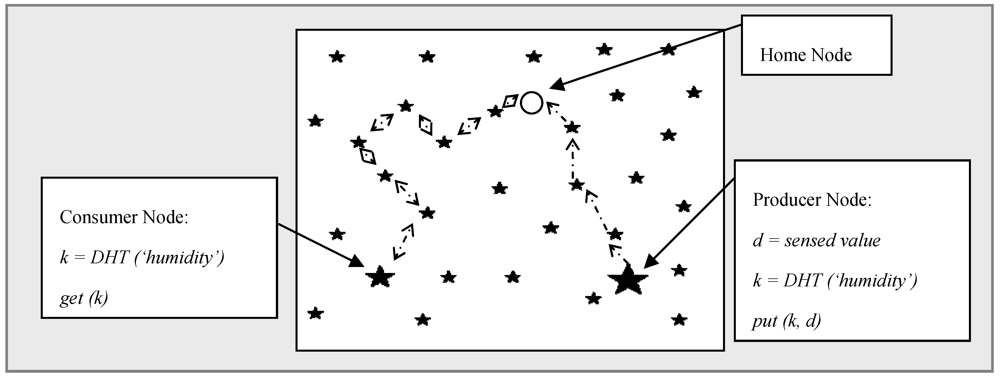
’. A producer node senses a value and forwards it to home node denoted by ‘ Jsan 01 00059 i002’. In turn, another consumer node uses the same hash function and retrieves the stored data from the home node. When storing data, represented by ‘ Jsan 01 00059 i004’, the producer node sends data to the target node and in the retrieval process, denoted by ‘ Jsan 01 00059 i005’, the query is first forwarded to the home node and replies are then sent back to consumer.
Figure 1. Geographic Hash Table [1].
Jsan 01 00059 g001

3.2. Similarity Data Storage (SDS)

Similarity Data Storage (SDS) [19] proposes an efficient spatial-temporal similarity search scheme for both static and dynamic WSN. Efficient data aggregation and query, similarity search for multi-attribute data and spatial temporal search are identified as three major challenges faced by DCS schemes. SDS is an important approach that utilizes spatial-temporal and similarity search functionalities and aims to reduce overhead, energy consumption and search latency. In SDS, a deployed large-scale WSN field is considered as a rectangular field. The entire field is divided into small rectangular zones. Each zone has a dedicated sensor node named as zone head. It is assumed that each node in the network is configured with three information elements: (1) Number of zones horizontally nx and vertically ny., (2) the zone ID assignments scheme—IDs are assigned within the zone sequentially from left to right, and (3) the zone ID and geographical location. A node in the zone with IDi can calculate its Euclidean distance from another zone IDj using Jsan 01 00059 i007, where δxi,j = (IDjIDi)%nx and δyi,j = (IDjIDi)/nx. A head node in a zone is responsible for communication with other zones. All other nodes inside a zone are connected with the head node.

3.3. Similarity Search Algorithm

The Similarity Search Algorithm (SSA) [22] was proposed by Chung, et al. based on the Hilbert Curve over a DCS structure. SSA is successful in searching similar data without collecting data from all of the network sensors. Being motivated from the Hilbert Curve concept, the authors divide the network recursively into 4l square quadrants where l denotes the number of levels. The center (indexing node) of each square quadrant (cell) is denoted by I. It is important to select the indexing nodes to avoid performance degradation due to too many indexing nodes and on the other hand a lack of enough storage space due to too few indexing nodes. If the total memory space for storing data is A and the memory size of each sensor is z, then the number of indexing nodes n can be defined as: Jsan 01 00059 i008
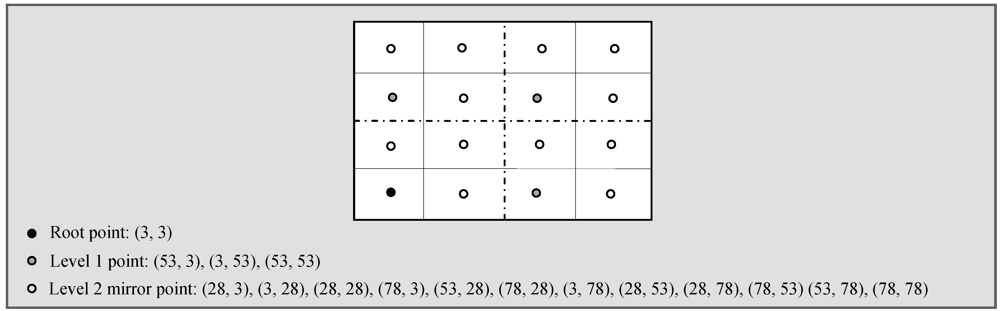
. So, the number of levels l is defined by: l = log4 Jsan 01 00059 i009. The entire data range of an event is referred to by R where RL and RU, respectively, denote the lower bound and upper bound. R is divided into n equal sub-ranges each being equal to r i.e., n.r = R. So, the data sub-range for which IID is responsible is defined as Jsan 01 00059 i010. Figure 2 illustrates level 1 and level 2 assuming that the data range R of an event is (0, 1). Detected events are mapped to a particular segment if the event falls in the range of that cell. Two parameters Jsan 01 00059 i011 are used to record the minimum and maximum values of each segment. Initially these two parameters are set to 0. When data is inserted into an index node, the values are updated accordingly. For example, if a sensor detects an event with a value of 0.2 then the data is sent to I0 as it belongs to the range [0, 0.25] and both parameters Jsan 01 00059 i011 of this cell will be updated to Jsan 01 00059 i012. Being a mini-repository of an entire distributed database, each sensor has knowledge of its local data and hence lacks global knowledge of the entire sensor database. The distributed nature of the data throughout the sensor network is one of the major challenges when processing similarity search queries. To overcome this challenge, the adjacent index nodes in SSA along the Hilbert curve have data of similar values and thereby avoid the need to collect data from all of the sensors in the network. This data mapping based on the concept of the Hilbert curve is simple and easy to implement. However, when storing multidimensional attributes it is not clear whether SSA maintains a separate Hilbert curve or not and in this case how it responds to the multidimensional queries.
Figure 2. Level 1 and Level 2 Hilbert Curve [22].
Jsan 01 00059 g002

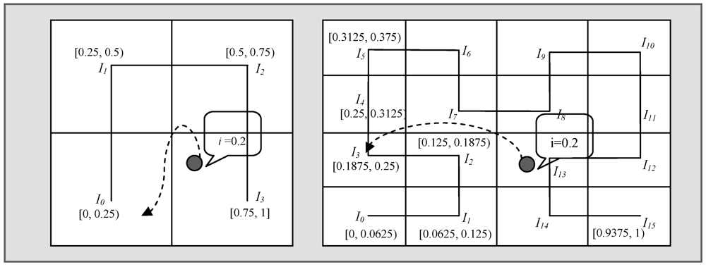
3.4. Dynamic Load Balancing

In Dynamic Load Balancing (DLB) [23], Liao, et al. mention unbalanced distribution of data among sensors as one of the major constraints for most of the DCS techniques. To address this issue, Liao, et al. propose a grid-based DLB approach that relies on two schemes: (1) A cover-up scheme to deal with the problem of a storage node whose memory space is depleted and (2) multi-threshold levels to achieve load balancing in each grid and all nodes get load balanced. DLB divides the whole network into a grid with cells of the same size in such a way that all the nodes inside a cell are within one hop distance. Each grid is numbered with positive coordinates (X, Y) called grid IDs. A sensor node can calculate its grid ID (X, Y) using the following equation:
Jsan 01 00059 i014 and Jsan 01 00059 i015    (1)
Each node has a virtual grid ID and virtual co-ordinates that are initially equal to the actual grid ID and co-ordinates. Initially, each node broadcasts a message within its grid by limited broadcast to exchange the information to build a ‘Grid_Node’ table. A producer node uses the hash function on the event type to map the event type into a grid and transform the event type into a grid ID using the above equation. The center of the grid is called a grid point. The node, after detecting an event, sends a Put packet to the grid ID and uses GPSR to forward this packet to the node closest to the grid point.

3.5. Load Balanced Data-Centric Storage

Load Balanced Data-Centric Storage (LB-DCS) [24] is an organic approach that relies on the home perimeter for data replication and thereby overcomes the unbalanced load constraint in DCS-GHT [1]. LB-DCS functions on top of three mechanisms: (i) A density estimation protocol that is used to estimate the network density f, which is included in put and get protocols; (ii) a modified hashing function that includes f in its parameter list; and (iii) a storage protocol enforcing QoS in the selection of the number of replicas for data storage. In [24,25], the authors show that depending on the event type, the number of local replicas should be different. So, when a producer node produces any event it also specifies a value in terms of the parameter q to specify the number of replicas. The put primitive takes q along with two other parameters: datum d and meta-datum k. Depending on the value of q, the home node selects q neighbor nodes using the ball method to replicate that event. This dispersal method is iterative. A home node, H (with co-ordinates XH, YH) considers a ball with a radius r (randomly selected value). The home node sends a request for storage to all sensors within the range of this ball denoted by:
Jsan 01 00059 i016    (2)
In turn, when a sensor receives a storage request it acknowledges the request to H. H calculates the number of acknowledgments (q') received from the nearest sensors. If q' < q, then H sends a storage request to Jsan 01 00059 i017 sensors. This time it considers only the sensors in Jsan 01 00059 i018. This process continues until H receives q acknowledgements or exhausts sensors within the perimeter. Apart from this QoS, the authors also include non-uniform hashing that can be used to balance the load even in non-uniform distribution such as a Gaussian distribution of sensor nodes in a network. In such a non-uniform WSN, LB-DCS applies two distributed protocols, referred to as proactive (Broadcast) and reactive (Stripes and Fatstripes), to compute the density approximation f of each zone. The density approximation is used to bias the hash function enabling the distribution of target co-ordinate pairs for storage according to the network distribution. For non-uniform hashing, the Rejection Method [26] has been used in LB-DCS.

3.6. Tug-of-War

In Tug-of-War (ToW) [27], the authors propose a data-centric mechanism where queries and events meet at a point that is selected based on the relative frequencies of events and queries. ToW operates in two modes referred to as write-one-query-all and write-all-query-one. The former allows a sensor to store an event in the nearest mirror image but queries need to be disseminated to all mirror images. Conversely, in the latter operation node events must be stored in all mirror images to facilitate a query node that disseminates the query to the nearest mirror image. ToW takes its motivation from the Structured Replication (SR) mechanism in GHT. In SR, to alleviate a node’s load, a detected event is stored in the nearest mirror image. This mechanism alleviates the storage cost but as a query node has no idea which image node may have the data, the query node needs to query all of the images and this increases the query cost. Like SR-GHT, a home node and a set of 4r1 mirror images are assigned in ToW for each event class c and here r is referred to as the system resolution. The mode a sensor node will operate depends on r. The system resolution is determined based on the relative query frequency and events detected for a particular class of event. To minimize the communication cost, ToW adjusts the rendezvous point on the fly on an optimal basis. With a given system resolution, nodes define the mode of operation while in the selected mode nodes need to find an optimal value of r in order to minimize the communication cost. In write-one-query-all mode, the total communication cost Jsan 01 00059 i019 per unit interval is defined by:
Jsan 01 00059 i020
Jsan 01 00059 i021    (3)
By using an optimal r, the cost of ToW in this mode per event is defined by:
Jsan 01 00059 i022    (4)
Here, Ce, Cq, fe, fq, k and n denote storage cost, query cost, event frequency, query frequency, number of the event detection node and total number of nodes deployed in the network, respectively. With the given value of k, fe, and fq, Jsan 01 00059 i023is minimized by the following value of r:
Jsan 01 00059 i024    (5)
Similarly, in write-all-query-one mode, the total communication cost is denoted by Jsan 01 00059 i025 and the optimal value of r is defined by:
Jsan 01 00059 i026
Jsan 01 00059 i027    (6)
Jsan 01 00059 i028    (7)
Using an optimal r, the cost of ToW in this mode per event is defined by:
Jsan 01 00059 i029    (8)
Thus, in order to determine the mode of operation, the resolution must be non-negative. With the given value of k, fe, and fq, if a nonzero optimal system resolution r exists in one mode then in other mode no non-zero optimal r can exist. Hence, finding a non-zero optimal r in a mode is essential to determine the mode of operation.

3.7. Quadratic Adaptive Replication

In Quadratic Adaptive Replication (QAR) [16], the authors recognize multi-replication as one of the most important DCS research areas and propose to enhance ToW by a flexible solution that permits selecting a more adaptive number of replicas. ToW is based on a geometric replication formula that calculates the number of replicas, Nr = 4d, where d is the network-depth. Thus, the main drawback of ToW is its inflexibility in selecting the number of replicas, which are limited to 1, 4, 16, 64, and so on. In contrast, QAR calculates the number of replicas as Nr = d2 allowing the number of replicas to grow in a quadratic fashion. Furthermore, QAR provides a mathematical model that can find the optimal number of rendezvous nodes based on the ratio of consumption and production traffic.

3.8. Double Rulings

Considering information brokerage as one of the prime concerns, the authors in [28] propose a Double Rulings scheme storing data replica at a curve instead of one or multiple isolated sensors. In this approach, information hints can be left along the trail when data travels from source to a rendezvous node at no extra communication cost. Hence, discovering relevant data also becomes easier for the consumer. The scheme provides greater flexibility to design a network’s retrieval strategy subject to the current network load and energy level. The paper presented a number of possible retrieval mechanism such as GHT retrieval, distance-sensitive retrieval, aggregated retrieval and double rulings retrieval. The flexibility in retrieval curves removes the possibility of having bottlenecks around the rendezvous node since the retrieval curve may not necessarily visit the rendezvous node. A local recovery scheme is achieved by storing data on the boundary when the sensors in a certain region are destroyed. Compared to SR-GHT, the double rulings scheme improves data robustness by imposing much lower communication costs for replication through the organization of replicas along a closed curve. The paper also proposed a new routing technique referred to as greedy routing on a curve, which adds extra complexity when implemented. Furthermore, flat replica in sensor nodes along the replication curve deplete the storage capacity of the network quicker than other schemes.

3.9. Distributed Erasure Coding in DCS

In contrast to pure replication, Michele Albano et al propose an alternate approach by incorporating erasure coding in DCS. In [29], the authors use the Redundant Residue Number System (RRNS) to encode data into a set of fragments based on n out of m code that guarantees the survival of the data in the event of the loss of a limited number of fragments (up to m-n). The put(d:k) primitive function first selects a set of sensors Nk to store the data based on the number of fragments to be computed, then it multicasts a storage request of d:k to the sensors in Nk.. Prior to sending the storage request, each sensor p (p belongs to Nk) is assigned with a module denoted by m(p), which is used to compute the fragments. The assigned module is randomly chosen from a library of m = n + r pairwise prime moduli m1,….,mn + r. Once a sensor p is assigned with a module m(p) for storing the pair d:k, it stores x:k in its memory where x is the fragment given by the residue of d module m(p). Upon receiving a request from a query node for data d:k stored by sensors in Nk, the reconstruction might happen using one of two strategies. In the first strategy, each sensor in Nk retrieves the fragment x:k that corresponds to d:k and sends it to the query node. In the second strategy, one sensor in Nk reconstructs d:k after collecting all of the fragments x:k from Nk and sends this reconstructed data to the query node. The first method ensures reliable data reconstruction at the cost of high energy consumption, on the other hand, the second method trades off energy consumption with reliability requiring only local communication in reconstructing the data, and only one final packet is sent to the sink.

3.10. Distributed Index for Features

Distributed Index for Features (DIFS) [30] in sensor networks is designed to provide communication load balance across the index keeping the search efficiency of a quad tree [31]. DIFS also uses a geographic hash similar to GHT [1]. DIFS constructs a multiply rooted hierarchical index that differs from traditional binary and quaternary trees. In DIFS, a non-root node can have multiple parents. Nodes are responsible for storing information for a specific range within a particular geographic region. A node covering a small area stores a wider range of values while a node covering a large area stores a smaller range of values. DIFS efficiently supports range queries related to values distributed in a range. Unlike QUAD tree, each child in DIFS has bfact parents where bfact = 2i, i ≥ 1. The range of values in the histogram of a child is bfact times the range of values maintained by its parents. The range of index values decreases by the factor bfact as it progresses up the index hierarchy. Suppose an event is detected and the value of an attribute (say flux density) is 57 and this attribute value is to be recorded in the index. This attribute value would be recorded in a local leaf node covering a range of 0~255 (considering the range of flux density 0~255) and would also be stored in the parent of the local leaf node that covers a range of 0~63, in a grandparent covering 48~63 and in a great grandparent with a value range of 56~59. Here, a value of bfact = 4 and hence the range of values covered by the grandparent is one fourth of that covered by the parent while the geographic area covered by grandparent is four times that of the parent and so on.
Figure 3. An Illustration of the Distributed Index for Features (DIFS) Hierarchy.
Jsan 01 00059 g003
In Figure 3, the width and height of the total covering region of a network is eight units (w = 8 and l = 8). Considering bfact = 2, the dimension of the system-specified minimum covering region for this case is 1 ( Jsan 01 00059 i031, where h is the number of levels) and 1 ( Jsan 01 00059 i032). Suppose that an event has been found in the vicinity of geographical co-ordinates (7.5, 4.5) with an attribute value of 8. For the time being, it is assumed that nothing is known a priori about the expected distribution of the attribute except that it always falls in the range [0~8]. The hash for the key “attribute:0:8” will return a location somewhere in the bounding box defined by the corner (7, 4) and (8, 5). So, a message containing the string “attribute”, the co-ordinates (7.5, 4.5) and the value 8 will be sent to leaf-level (level 0) index node, say Jsan 01 00059 i033. Since, bfact = 2, the level 0 leaf index node will forward a histogram containing a count for values 7~8 to a level 1 index Jsan 01 00059 i034covering the region (6, 4) to (8, 6). The level 1 node will then forward a histogram containing counts for values 4~8 to a level 2 node, Jsan 01 00059 i035 covering the region (4, 4) to (8, 8). This process continues until the value is forwarded to node Jsan 01 00059 i036covering the entire network bounded by (0, 0) and (8, 8).
DIFS provides communication efficiency and fast searching of data by name, value range and location. Furthermore, a communication bottleneck at the root of the search tree is avoided using multiple parents of a child thereby maintaining the search efficiency that can be achieved by drilling down through a search tree using a hierarchical approach.

3.11. Practical Data-Centric Storage

In PathDCS [32] messages are routed to locations using a tree-structure, and the path to a location is identified using landmarks, which are shared reference points. The interesting novelty of this approach is that an event type is mapped to a path instead of mapping the event type to a spatial location. The path is defined by an initial landmark and then followed by a set of procedural directions. The landmarks are also called beacon nodes, which are elected randomly or manually configured. Standard tree construction techniques are used to build trees rooted at each of these beacon nodes. This ensures that all nodes know how to reach the beacons. A path consists of a sequence of bi pairs (bi, li), where bi is a beacon and li is a length. A beacon node bi is the beacon whose identifier is closest to the hash function h(k, i). The packet is first routed to beacon b1, and then it is sent l2 hops toward beacon b2 using the tree rooted at b2, and so on, until it arrives at the previous i 1 segment. The packet is then sent li hops toward the next beacon bi. In addition, the first segment length l1 is equal to the distance to the first beacon b1, whereas segment lengths for i > 1 are given by:
Jsan 01 00059 i037    (9)
The PathDCS algorithm has two parameters: the total number of beacon nodes denoted by B and the number of path segments P. The performance of PathDCS largely depends on these two parameters and by varying the number of B, PathDCS trades off the control traffic overhead due to tree construction versus load on the beacons. Data is also been locally replicated by flooding within k-hops of the destination.

3.12. Hierarchical Voronoi Graph Based Routing

A Hierarchical Voronoi Graph Based Routing (HVGR) [33], the Voronoi graph is used to construct and maintain a virtual hierarchy of sensor nodes. The Voronoi approach is a self-organizing hierarchical graph that is constructed without the help of GPS or other geo-location devices. The network is divided into different levels of regions based on landmarks. A landmark selection algorithm is used to select at most mi(i = 1, 2, ….) landmarks in an (i 1)th level region. Then the network is divided into first level sub-regions based on first level landmarks. Each node in the first level sub-regions broadcasts a landmark packet to the entire network. By receiving this packet every node estimates its distance from all first level sub-region landmarks. Each node selects one landmark as its representative. Then each first level sub-region is again divided into second level sub-regions with second level landmarks. Each sensor node again chooses the closest landmark as its second representative. This process continues until the last level sub-regions are small enough so that each node knows all other nodes in its sub-region as shown in Figure 4.
Figure 4. Region Oriented Routing [33].
Jsan 01 00059 g004
For landmark selection the authors use the optimized random landmark selection algorithm [34]. According to this algorithm, a random node, say ‘L1, starts the landmark selection process becoming the master landmark of first level landmark nodes. It then selects m11 nodes for m1 first level networks. Each first level landmark then again acts as master and continues the selection process in its zone to select a second level master node for the second level of the network. A master landmark node stops the landmark selection process once it finds that all sensor nodes in its region are within its communication range. Figure 4 shows an example of the basic routing algorithm that is used to route packets from the source (S) to the destination (D). The first level landmark for the destination is L1. The packet first moves hop by hop toward L1 until it reaches the edge of first level region, R1. Now, nodes in R1 know the second level landmark and the packet now moves hop by hop toward the second level landmark, L2. Again once it reaches the node B of region 2 in Figure 4, the packet starts moving toward L3. Finally, the packet reaches the lowest level sub region whose entry node ‘C’ knows the path of the destination and forwards the packet to the destination. The interesting part of this algorithm is it never overwhelms the landmark, as the packets never go to the landmark, rather the packets move toward the landmark until the packets reach any node within the region.

3.13. Data Storage and Range Query for Multidimensional Attribute

Multidimenstional Attribute (MDA) [35] proposes an energy-efficient & scalable multi-dimensional range query mechanism (MDAs) to retrieve and store data. It builds an in-network distributed data structure by mapping multi-dimensional attributes to their corresponding range spaces. The authors consider a few assumptions in their work: (1) The sensors are uniformly and densely deployed; (2) each node can sense multiple events; and (3) each node maintains a neighbor table via periodic beacon message exchanges and knows its own geographic location. A source node detects an event with a set of attribute values, E = {a1, a2... an}. It is assumed that all attribute values are scalar and normalized to (0~1). An event is assigned with a k bit code where k = 2m. If 0 < ai < 0.5, the ith bit code is assigned to 0 otherwise 1. For xj=a2j-1 and yj=a2j the attribute values of E are assigned by a serial bit code B = {x1, y1, x2, y2……xm, ym}. For example, an event E = {0.8,0.7,0.4,0.3} is assigned by a four bit code B={ x1, y1, x2, y2}={1,1,0,0}. Assignment of code B can be achieved by generalizing 0 < ai < 0.5 and 0.5 < ai < 1 to 0 < 2ai < 1 and 1 < 2ai < 2, respectively:
Jsan 01 00059 i038
Jsan 01 00059 i039    (10)
Jsan 01 00059 i040
Jsan 01 00059 i041    (11)
This code B is mapped to a range space R = [xlowxup, ylowyup]. Hence, it is necessary to calculate (xlow, ylow) and (xup, yup) to find the range space R.
In code B, x = x1, x2… xm are used to calculate X of R and y = y1, y2… ym are used to calculate Y of R. In code B, if x1 = 1 its value is in between 0.5 and 1; if x2 = 1 its value is in between 0.5 and 0.5 + (0.5)2. So, Xlow = x1(0.5) + x2(0.5)2 + ……. + xm(0.5)m. Similarly Ylow = y1(0.5) + y2(0.5)2 +……. + ym(0.5)m.
Again, Xup is defined by:
Xup= 1 − (x1(0.5) +x2(0.5)2 +……. + xm(0.5)m)
So, Jsan 01 00059 i042
Jsan 01 00059 i043
So, Jsan 01 00059 i044
Jsan 01 00059 i045
Jsan 01 00059 i046    (12)
Example:
Jsan 01 00059 i047
Jsan 01 00059 i048
Jsan 01 00059 i049
Jsan 01 00059 i050
Jsan 01 00059 i051
Jsan 01 00059 i052
Jsan 01 00059 i054
Jsan 01 00059 i055
Jsan 01 00059 i056
Jsan 01 00059 i057
Hence, the range space is defined by R = (0.5–0.625, 0.875–1). Figure 5 illustrates the MDAs storage and query process.
Figure 5. Multidimensional Range Query Mechanism (MDAs) [35].
Jsan 01 00059 g005

4. Classification Based on Taxonomy and Design Drivers

4.1. Range Query

In [13,19,22,30,35,36], the range query mechanism is implemented in different format. Chung et al. [22] propose an efficient technique, illustrated in Section 3.3, for a DCS similarity search that includes both a point and range query. A range query is divided into sub-queries and then the sub-queries are forwarded to their corresponding indexing node. For example, the level of carbon monoxide found in the air in a forest may be represented by levels that range from 50 L/mol to 150 L/mol. This range is split equally into four (41=4, four index node referred as I0, I1, I2, I3) sub-ranges [50, 75), [75, 100), [100, 125), [125, 150]. Hence, if a range query is to find data within [60, 80), then the sub-ranges of I0 and I1 are located as they cover the given query.
Li, et al. [13], proposed a method called DIM, which includes both a point and a range query in a multidimensional DCS model. In DIM, each sensor is linked as a node in a tree structure where each node represents a range of values. A root node represents the entire range of values and splits into two equal parts for left and right child nodes. This process continues for each non-leaf node until leaf nodes are reached.
DIFS [30], referring to Section 3.10, performs a data fusion based on data conveyance through the network. The routing is designed on top of a quad tree in a manner that balances the communication load across the index, and the range is maintained along the sensor node hierarchy.
In MDA [35], described in Section 3.13, a range query is split into a k-dimension range of multiple sub-queries. After splitting, each attribute sub-query is assigned with a bit code and tuples of k-bit codes, referred to as code B, are produced. The code B are then mapped to range space R and data is stored in nodes located in the mapped R. The state-of-the-art approaches in the field of range query DCS are summarized in Table 1.
Table 1. Summary of Range-Query Data-Centric Storage (DCS) Schemes.
MechanismsSchemes
Bit Code MappingMDA [35]
Tree StructureMultiply Rooted Hierarchical IndexDIFS [30]
Binary TreeDIM [13]
OthersSSA [22]

4.2. Similarity Search

In SDS [19], described in Section 3.2, a data item denoted by d consists of keywords denoted by vd. Thus, the data item d is represented by d = (v1d, v2d,………, vmd). For a similarity search, the following formula is proposed in SDS to calculate the similarity between data items d1 and d2:
Jsan 01 00059 i059    (13)
Here, m is the number of attributes, wi is the weight for each attribute based on their significance as shown in Table 2 and B(i, j) is a Boolean function returning 1 if vid1=vid2 and 0 otherwise.
Table 2. Example of Weight Settings [19].
AttributeKeywordsWeight
ObjectCar, Plane, Truck, etc.0.3
ModelF-16, F-17, etc.0.2
ColorRed, Purple, etc0.1
DirectionNorth, South, etc0.1
DivisionAir-Force, etc.0.1
PressureInteger0.1
SpeedFloat0.1
......
For example, a data item in a WSN application is characterized by five attribute lists such as object, model, color, direction and division with the weight value shown in Table 2. Consider the following two data items denoted by d1 and d2:
Jsan 01 00059 i060
Jsan 01 00059 i061
Hence,
Jsan 01 00059 i062
SDS uses Locality-Sensitive Hashing (LSH) [37] to transform d to a series of hash values. Using LSH, data items that have common keywords will have the same hash value while similar data items will have similar hash values. For example, if the difference between d1, d2, and d3 is d1 > d2 > d3, their hash values conform to hd1 > hd2 > hd3, where hd is the hash value of d. A data item with a hash value h is mapped to the first zone with ID ≥ h. For example, if the value of hd1returned by LSH is five, then the value of hd2 (d1 and d2refer to the data item shown above) would approximately be 6.67 or 3.75. Hence, d1 will be stored in the zone with ID ≥ 5 and d2 will be stored in the zone with ID ≥ 3.75 or ID ≥ 6.67. Thus, a query denoted by dq with 80% similarity will search in zones with IDs: Jsan 01 00059 i063.
In SSA [22], referring to Section 3.3, when data is queried, the query is first sent to the specific cell, with the range of this cell in the queried data. The SSA similarity search mechanism contains two phases known as the similarity search query resolving phase and the query probing phase. The query resolving phase determines an indexing node that is most likely to provide an answer for the query. If the answer does not match exactly then the query probing phase is initiated to find the closest possible answer.
In the query resolving phase, the function locate (Vq) is used to find the target node IT with the indexing node IID such that RL + (IID− 1)∙r Vq < RL + IID∙r, where Vq is the search value given by the query. The query is then forwarded to the Target Node IT to retrieve data. If an exact match to Vq is found, then the query execution is finished, otherwise the query probing phase comes in action. In the query probing phase there can be the two following possible cases:
  • Case 1: IT is non-empty and vIT s is the most similar local data in IT.
    • ○ Sub-case 1: If vIT s is larger than vq, then all data in IT+1 must be even greater than vq. But in IT-1 there may be a Jsan 01 00059 i064 that is closer to vq.
    • ○ Sub-case 2: If vIT s is smaller than vq, then all data in IT-1 must not be more similar to Jsan 01 00059 i065 than vIT s is. But in IT+1 there may be a vIT+1 s that is closer to vq.
  • Case 2: IT is empty (i.e., no data stored). vq has to be sent to both neighbors (i.e., IT1 and IT+1) of IT to find the most similar data.
In SSA, three functions are proposed referred as backward probing, forward probing and bi-directional probing where backward probing and forward probing are used to deal with Case 1 and bi-directional probing is used for Case 2.

4.3. Data Aggregation

In [38], the authors propose four application profiles where two are aggregation profiles called ConsAggr and ProdAggr. Data aggregation is proposed using replication nodes proposed in QAR, see Section 3.7. In ConsAggr the profile consumer queries dominate production queries. In this profile, events produced in a given area are aggregated using the replication node for that area. In contrast, with the ProdAggr profile the production traffic dominates consumption traffic. Replicas aggregate events received from producers to achieve an effective overall traffic reduction. In Resilient Data Centric Storage (RDCS) [36], three types of event query called List, Summary and Attribute-based are proposed for the DCS scheme. A query request for all stored data for a particular event type is referred to as a List while a query request for aggregated or summarized data for a particular event type is called a Summary query. On the other hand, an Attribute-based query requests data for all events that match certain constraints based on attribute values. However, it is not mentioned how the monitor node will aggregate data for an event type to give a response to the summary query. TinyDB [9], madwise [39] and TAG [40] are some of the aggregation mechanisms proposed mainly for WSN databases, which can be adapted to DCS networks as well.

4.4. Sensor Network Field Non-Uniformity

Load Balanced Data Centric Storage (LB-DCS) [24], Section 3.5, deals with non-uniformity of the sensor network based on two mechanisms. At first it estimates network distribution and then exploits data dissemination methods based on the estimation. A closest sensor node, called the sentinel, to the watch point, which is the region center, is responsible to identify its neighbors by sending broadcast messages. Every sentinel node sends its own region’s sampling density estimation toward other sentinel nodes using both proactive (Broadcast) and reactive protocols (Stripes and FatStripes).

4.5. Multi-Replication

From GHT on [1], illustrated in Section 3.1, a home node is called a hotspot if too many events with the its key are detected. To address this issue the authors have extended GHT by employing Structured Replication (SR) referred to as SR-GHT. SR-GHT introduces a hierarchical scheme where one node can have 4d− 1 mirror images of the root home node.
Figure 6. Structured Replication [1].
Jsan 01 00059 g006
The hierarchy depth is denoted by d. As shown in Figure 6, a decomposition of two (d = 2) is deployed having 42− 1 (15) mirror images at different levels. A producer node can store the detected event to its closest mirror node reducing the storage cost to Jsan 01 00059 i066 from Jsan 01 00059 i067. In the retrieval phase, GHT needs to forward queries to all mirror images. The query is first sent to the root node, which then forwards it to all mirror images in level 1 and then level 1 nodes forward this query to level 2 mirror images. This again increases the retrieval cost to Jsan 01 00059 i068 from Jsan 01 00059 i066. Table 3 shows a summary of multi-replication DCS schemes based on their functionalities.
Table 3. Summary of Multi-Replication DCS Schemes.
SchemesPolicyRoutingAmong Replica NodesRemark
1SR-GHT [1]Hierarchical Grid Replication Mechanism (4d)Recursive HierarchicalAs data never replicated to all nodes, basic data lost problem exists
2SDS [19]Head node stores copy of all client dataN/ASingle point of head zone failure. Head zone energy depletes quicker than others
3ToW [27]Hierarchical Grid Replication Mechanism (4d)CombingExtends SR-GHT by adding two modes of operation. It inherits drawbacks from SR-GHT
4SSA [22]Create mirror of index node using Mirror Hilbert Curve & Mirror Mapping FunctionNot SpecifiedIt doesn’t explain how data would be mirrored rather just a proposal is mentioned by couple of lines
5RDCS [36]Each zone has at most one replica node of mirror nodeGPSRSelection of mirror node is not specified clearly.
6QAR [16]Hierarchical Grid Replication Mechanism with Quadratic Evolution (d2)CombingInherits drawbacks from SR-GHT
6Double Rulings [28]Stores data replica at a curve instead of one or multiple isolated sensorsGreedy Routing on a CurveCan only employ 2 global replicas while tow and qar are adaptable to traffic load with multiple replicas
7Dynamic Random Replication [41]Replicate data in randomly selected set of data replication nodesMinimum Spanning TreeTwo major limitations: static WSN and consideration of homogenous spatial applications
In SDS [19], Section 3.2, the head node keeps a copy of all data to be replicated, which may be unrealistic due to storage space availability, and if any head node fails, then data cannot be recovered from the head node. ToW [27] also replicates the root node into 4d− 1 mirror images like GHT but the authors used a combing routing protocol, taking advantage of the grid structure (see Figure 6) to create a shorter replication tree for transferring messages among replica nodes. Like GHT and ToW, QAR also proposes replication of the home node but in a more adaptable quadratic evolution Nr = d2. QAR also provides an analytical model defining the optimal number of replicas (Nr*), thus minimizing the overall network traffic. However, Unlike GHT, ToW and QAR replicate producer data to all replicas in their second mode of operation. Nevertheless, the mode of operation is not deterministic since the mode of operation depends on the resolution (see Section 3.6) and hence ToW and QAR might also suffer from the data loss problem during their first mode of operation, i.e., write_one_query_all. SSA [22] creates a mirror of the index node using a mirror Hilbert Curve and mirror mapping function. However, the replication process is not explained in the paper. RDCS [36] proposes at most one mirror node for each zone, which will keep a copy of the zone’s index node. An index node stores all data directed toward its responsible zone and therefore creation of a hotspot surrounding the index node is possible. Nevertheless, the hotspot issue has not been mentioned in the selection process for the mirror node. Dynamic random replication for DCS [41] and double rulings [28], described in Section 3.8, are two important research outcomes related to multi-replication research for DCS. Relative to previous work, random replication is a simpler and more flexible technique that enables an effective reduction of network traffic. The schemes, specifically, consider the case where nodes can determine the current set of Nr replicas associated with a given application by generating Nr random spatial locations with a hash function Jsan 01 00059 i069, where app is the application’s name and epoch is a shared time identifier employed to change replicas over time. The paper demonstrates that by placing a replica node randomly in the network it is possible to outperform ToW, QAR and GHT. Also by changing replication nodes over time it is possible to equalize the energy burdens across the network and hence a 60% improvement in network lifetime may be possible. However, the wireless network in the model is assumed to be static and the application is considered to be spatially homogenous.

4.6. Load Balancing

In DLB [23], Section 3.4, to balance the load among sensors in a grid, a scheme named the ‘cover-up’ scheme is used. According to this scheme every node of a grid has storage threshold levels. For instance, a sensor node has two threshold levels, e.g., 1st level = 30 and 2nd level = 60. A grid point forwards packets to the closest grid node for storage. When the node closest to the grid point reaches the first threshold level it modifies its virtual co-ordinate to (∞, ∞) in order to hide its original location. Hence, the geographic routing protocol forwarding event data to a storage node will ignore the original closest node and find a new node that is the next closest node to the grid point. This process continues until all nodes reach their first threshold level. The last node, farthest from the center, reaching this threshold broadcasts that the first threshold has been reached and the second threshold storage level is established. However, following this mechanism, at some point,all of the nodes within a grid could become saturated. If this occurs, the paper proposes an extended grid that uses adjacent grids to the saturated one to select a new home node.
The authors introduce two types of load balancing schemes in SDS [19]: (1) storage load balancing and (2) routing load balancing. In storage load balancing, the storage load is balanced among different zones. Every zone maintains a threshold, denoted by φ, of the percentage of a zone’s used storage to indicate when a zone is at risk of being overloaded. When a zone’s storage crosses φ, it starts forwarding all storage requests to a lightly loaded neighbor zone. Every zone calculates its storage status Jsan 01 00059 i070and forwards this status to its neighbor zones periodically. In routing load balancing instead of routing packets using one specific route, SDS calculates more than one shortest route between a source or relay and destination. This reduces congestion in any specific route. The calculated shortest path between Ha (Xa, Ya) and Hb (Xb, Yb), as shown in Figure 7, is not unique. For simplification let us consider |XaXb| = |YaYb| and then the maximum number of inflexion points in the horizontal and vertical routing process is C = |XaXb|∙C. The number of choices in choosing j inflexion points among C is Jsan 01 00059 i071, which is equivalent to the problem of putting C ball into j boxes. There are 2j possible routes for each choice with j inflexion points, hence the maximum number of possible shortest routes between Ha and Hb is Jsan 01 00059 i072. When two nodes frequently communicate to each other, each query issuer randomly chooses one at each time from the list of all the shortest paths calculated.
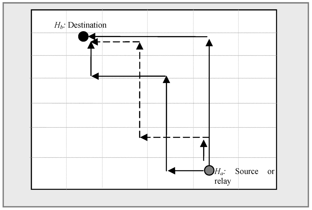
Figure 7. Multiple Shortest Routes [19].
Jsan 01 00059 g007
In HVGR [33], Section 3.12, for balancing the load among sensor nodes, the name based routing approach is modified. During the landmark selection, the network is divided unevenly. For example, an event E has a probability 1/m1 of being assigned to the first level landmarks (L1, L2,…). If the network is divided unevenly (L1 > L2), L2 is more likely to be overloaded earlier than L1. Hence the load is balanced by assigning a task to regions in proportion to the region size. An event is stored in a node in Lks first level region if:
Jsan 01 00059 i074    (14)
Here, Ni is the number of nodes in landmark Li’s first level region and Jsan 01 00059 i075.
In LB-DCS [24], for handling load balancing across a dynamic network, the hash function includes a network density estimation f. To estimate sensor density, the WSN is divided into n x n non-overlapping square regions with a side length p. A sensor node closest to the center of a zone is referred to as a watch point and is called a sentinel node. Each sentinel node broadcasts a request to its neighbors to count them. The number of neighbors is used as an estimation of the local density in the region. One proactive (Broadcast) and two reactive protocols (Stripes and FatStripes) are used to deliver the estimate computed by sentinels to other sensor nodes. After collecting estimates a sensor uses Jsan 01 00059 i076and Jsan 01 00059 i077to calculate the density in each region and the final approximation based on the first computation, respectively. Here, wij is the density estimated by the sentinel for the i, j region and m is the number of neighbors in this region. In two situations referred to as false zeroes and over reporting, d ' i,j might give a misleading density estimation value. A region with sparse nodes near the watch point or a concentration of nodes near the border may report a zero or very low density representing false zeroes. In another situation, a region with a high concentration of nodes near a watch point and sparse nodes near borders may report a higher density than normal representing over reporting. To overcome these situations the final approximation di,j is computed as a weighted mean of the approximation computed in the first step for region ij. Table 4 shows a summary of load balancing DCS schemes based on their functionalities.
Table 4. Summary of Load Balancing DCS Schemes.
FunctionalitiesSchemesMethod Used
Intra-Zone Load BalanceDLB [23]Cover-up Scheme
Inter-Zone Load BalanceSDS [19]Measuring Storage Usage Status ( Jsan 01 00059 i078)
DLB [23]Extended Grid (Cover up grid)
HVGR [33]Proportional Assignment of Storage Task to Regions
LB-DCS [24]Sampling Density, Broadcast, Stripes, FatStripes
KDDCS [42]Weighted Split Median
Routing Load BalanceSDS [19]Distributing Routing Load to All Possible Routes Equals to Jsan 01 00059 i079

4.7. Routing Algorithm

The DCS scheme might incur high update traffic due to the lack of an optimally synchronized routing algorithm. Initial research in DCS focused on designing an efficient technique that could be used to map data to the rendezvous node/zone rather than concentrating on developing an optimal packet routing technique. Most of the DCS methods, for data storage and search routing, rely on a locating system (e.g., GPS) that places an energy burden on the WSN. However, in the last quarter of this decade a few DCS techniques were proposed putting focus on enhancement of packet routing. These different routing algorithms can broadly be divided into two categories namely point-to-point routing and tree based hierarchical routing. In point-to-point routing the deployed network field is divided into zones or sectors and data usually propagates from one zone or rendezvous node to another in a multi-hop point-to-point fashion. In contrast, tree based hierarchical routing relies on a tree-construction technique dividing the whole network into a tree-structure and provides a mapping of data transfer paths with minimal assumption about the underlying infrastructure. DIM [13], KDDCS [42] are developed based on K-D trees while HVGR [33] and PathDCS [32] were developed on top of hierarchical Voronoi Graph and path based tree structure respectively. Table 5 summarizes DCS schemes based on these two types of routing algorithm used.
Table 5. Summary of DCS Schemes Based on Routing Algorithm.
Routing AlgorithmSchemes
Point-to-Point RoutingGPSRMDA [35], GHT [1], DLB [23], DIM [13], D-GHT [43], LB-DCS [24], Q-NIGHT [25], SSA [22], Tug-of-War [27], RDCS [36]
Logical Stateless Routing (LSR)KDDCS [42]
CAR-POOLINGSDS [19]
COMBINGTug-of-War [27]
Recursive Hierarchical RoutingSR-GHT [1]
Tree Based Hierarchical RoutingGPSRDIFS [30], DIM [13]
PATH BASED TREE STRUCTUREPathDCS [32]
HIERARCHICAL VORONOI GRAPH BASED ROUTINGHVGR [33]
VPCRGEM [44]

5. Conclusion

As it has become apparent, significant research has occurred since 2002 on WSN DCS schemes. Since WSN may be deployed in large-scale networks with thousands of sensors, efficient data storage and retrieval mechanisms are of pivotal importance. The key DCS schemes have been classified in this paper and summarized for convenience in Table 6. In the current literature, identified DCS schemes do not provide solutions for all the challenges mentioned in Section 2. Some key challenges such as similarity, spatial-temporal similarity search and the non-uniformity of sensor networks are addressed only in a few papers and conclusive approaches are yet to be found. Other challenges are still open.
Table 6. Summary of DCS Schemes Highlighting Their Key Features.
TitleRouting CategoryDimension (attribute)Range vs. Point QueryData AggregationSimilarity SearchMulti ReplicationLoad Balance
1Geographic Hash Table (GHT) [1]Point-to-PointRoutingSinglePointNoNoNoNo
2Data Storage and Range Query Mechanism for Multi-dimensional Attributes. [35]Point-to-PointRoutingMultiRangeNoNoNoNo
3Distributed Spatial-Temporal Data Storage Scheme. [19]Point-to-PointRoutingMultiRangeNoYesNoYes
4Load Balanced and Efficient Hierarchical Data-Centric Storage. [33]Point-to-Point RoutingSinglePointNoNoNoYes
5Dynamic Load Balancing Approach [23]Point-to-Point RoutingSinglePointNoNoNoYes
6Load Balanced Data-Centric Storage (LB-DCS) [24]Point-to-Point RoutingSinglePointNoNoNoYes
7Tug-of-War [27]Point-to-Point RoutingSinglePointNoNoYesNo
8Efficient Mechanism for Similarity Search [22]Point-to-Point RoutingSingleBothNoYesNoYes
9DIFS: A Distributed Index for Features in Sensor Network [30]DCS Based on Tree-StructureSingleRangeNoNoNoNo
10PathDCS [32]DCS Based on Tree-StructureSinglePointNoNoNoNo
11DIM [13]DCS Based on Tree-StructureMultiBothNoNoNoNo
12GEM [44]DCS Based on Tree-StructureSingleRangeNoNoNoNo
13KDDCS [42]DCS Based on Tree-StructureSingleRangeNoNoNoYes
14RDCS [36]Point-to-Point RoutingSingleRangeYesNoNoNo
15Modeling Data Aggregation [38]Point-to-Point RoutingSingleN/AYesNoYesNo
There is also a strong need to have an efficient compatible routing algorithm specifically designed for DCS. Most DCS schemes utilize GPSR routing and research is occurring into developing routing protocols based on tree and hierarchical structures. An optimal approach for large WSN is yet to be found.

References

  1. Ratnasamy, S.; Karp, B.; Yin, L.; Yu, F.; Estrin, D.; Govindan, R.; Shenker, S. GHT: A Geographic Hash Table for Data-centric Storage. In Proceedings of the 1st ACM International Workshop on Wireless Sensor Networks and Applications, Atlanta, GA, USA, 28 September 2002; pp. 78–87.
  2. Campobello, G.; Leonardi, A.; Palazzo, S. A Novel Reliable and Energy-Saving Forwarding Technique for Wireless Sensor Networks. In Proceedings of the Tenth ACM international Symposium on Mobile Ad Hoc Networking and Computing, New Orleans, LA, USA, 18-21 May 2009; pp. 269–278.
  3. Pottie, G.J.; Kaiser, W.J. Wireless integrated network sensors. Commun. ACM 2000, 43, 51–58. [Google Scholar] [CrossRef]
  4. Saroiu, S.; Gummadi, P.K.; Gribble, S.D. A Measurement Study of Peer-to-Peer File Sharing Systems. In Proceedings of the Multimedia Computing and Networking (MMCN), San Jose, CA, USA, January 2002; pp. 152–157.
  5. Yao, Y.; Tang, X.; Lim, E.-P. In-Network Processing of Nearest Neighbor Queries for Wireless Sensor Networks. In Proceedings of the 11th International Conference on Database Systems for Advanced Applications, Singapore, 12–15 April 2006; pp. 35–49.
  6. Szewczyk, R.; Polastre, J.; Mainwaring, A.; Culler, D. Lessons from a Sensor Network Expedition. In Proceedings of European Workshop Wireless Sensor Network, Berlin, Germany, 19-21 January 2004; pp. 307–322.
  7. Intanagonwiwat, C.; Govindan, R.; Estrin, D. Directed Diffusion: A Scalable and Robust Communication Paradigm for Sensor Networks. In Proceedings of the 6th Annual International Conference on Mobile Computing and Networking, Boston, MA, USA, 6-11 August 2000; pp. 56–67.
  8. Zhang, W.; Cao, G.; Porta, T.L. Data dissemination with ring-based index for wireless sensor networks. IEEE Trans. Mob. Comput. 2007, 6, 832–847. [Google Scholar] [CrossRef]
  9. Madden, S.R.; Franklin, M.J.; Hellerstein, J.M.; Hong, W. TinyDB: An acquisitional query processing system for sensor networks. ACM Trans. Database Syst. 2005, 30, 122–173. [Google Scholar] [CrossRef]
  10. Ye, F.; Luo, H.; Cheng, J.; Lu, S.; Zhang, L. A Two-tier Data Dissemination Model for Large-scale Wireless Sensor Networks. In Proceedings of the 8th Annual International Conference on Mobile Computing and Networking, Atlanta, GA, USA, 23-26 September 2002; pp. 148–159.
  11. Ye, F.; Zhong, G.; Lu, S.; Zhang, L. Gradient broadcast: A robust data delivery protocol for large scale sensor networks. Wirel. Netw. 2005, 11, 285–298. [Google Scholar] [CrossRef]
  12. Langendoen, K. Medium access control in wireless sensor networks. Medium Access Control Wirel. Netw. 2008, 2, 535–560. [Google Scholar]
  13. Li, X.; Kim, Y.J.; Govindan, R.; Hong, W. Multi-dimensional Range Queries in Sensor Networks. In Proceedings of the 1st International Conference on Embedded Networked Sensor Systems, Los Angeles, CA, USA, 5-7 November 2003; pp. 63–75.
  14. Ganesan, D.; Estrin, D.; Heidemann, J. DIMENSIONS: Why do we need a new data handling architecture for sensor networks? ACM SIGCOMM Comput. Commun. Rev. 2003, 33, 143–148. [Google Scholar] [CrossRef]
  15. Ganesan, D.; Cerpa, A.; Ye, W.; Yu, Y.; Zhao, J.; Estrin, D. Networking issues in wireless sensor networks. J. Parallel Distrib. Comput. 2004, 64, 799–814. [Google Scholar] [CrossRef]
  16. Rumín, Á.C.; Pascual, M.U.; Ortega, R.R.; López, D.L. Data centric storage technologies: Analysis and enhancement. Sensors 2010, 10, 3023–3056. [Google Scholar] [CrossRef]
  17. Chatzigiannakis, I.; Kinalis, A.; Nikoletseas, S. An Adaptive Power Conservation Scheme for Heterogeneous Wireless Sensor Networks with Node Redeployment. In Proceedings of the Seventeenth Annual ACM Symposium on Parallelism in Algorithms and Architectures, Las Vegas, NV, USA, 17-20 July 2005; pp. 96–105.
  18. Shih, K.P.; Wang, S.S.; Chen, H.C.; Yang, P.H. CollECT: Collaborative event detection and tracking in wireless heterogeneous sensor networks. Comput. Commun. 2008, 31, 3124–3136. [Google Scholar] [CrossRef]
  19. Shen, H.; Zhao, L.; Li, Z. A distributed spatial-temporal similarity data storage scheme in wireless sensor networks. IEEE Trans. Mob. Comput. 2011, 10, 982–996. [Google Scholar] [CrossRef]
  20. Rowstron, A.I.T.; Druschel, P. Pastry: Scalable, Decentralized Object Location,and Routing for Large-Scale Peer-to-Peer Systems. In Proceedings of the IFIP/ACM International Conference on Distributed Systems Platforms, Heidelberg, Germany, 12-16 November 2001; pp. 329–350.
  21. Karp, B.; Kung, H.T. GPSR: Greedy Perimeter Stateless Routing for Wireless Networks. In Proceedings of the 6th Annual International Conference on Mobile Computing and Networking, Boston, MA, USA, 6-11 August 2000; pp. 243–254.
  22. Chung, Y.-C.; Su, I.F.; Lee, C. An efficient mechanism for processing similarity search queries in sensor networks. Inf. Sci. 2011, 181, 284–307. [Google Scholar] [CrossRef]
  23. Liao, W.-H.; Shih, K.-P.; Wu, W.-C. A grid-based dynamic load balancing approach for data-centric storage in wireless sensor networks. Comput. Electr. Eng. 2010, 36, 19–30. [Google Scholar] [CrossRef]
  24. Albano, M.; Chessa, S.; Nidito, F.; Pelagatti, S. Dealing with nonuniformity in data centric storage for wireless sensor networks. IEEE Trans. Parallel Distrib. Syst. 2011, 22, 1398–1406. [Google Scholar] [CrossRef]
  25. Albano, M.; Chessa, S.; Nidito, F.; Pelagatti, S. Q-NiGHT: Adding QoS to Data Centric Storage in Non-Uniform Sensor Networks. In Proceedings of the 2007 International Conference on Mobile Data Management, Mannheim, Germany, 7-11 May 2007; pp. 166–173.
  26. Von Neumann, J. Various techniques used in connection with random digits. Appl. Math Ser. 1951, 12, 36–38. [Google Scholar]
  27. Joung, Y.-J.; Huang, S.-H. Tug-of-War: An Adaptive and Cost-Optimal Data Storage and Query Mechanism in Wireless Sensor Networks. Lect. Note. Comput. Sci. 5067, 237–251. [Google Scholar]
  28. Sarkar, R.; Zhu, X.; Gao, J. Double Rulings for Information Brokerage in Sensor Networks. In Proceedings of the 12th Annual International Conference on Mobile Computing and Networking, Los Angeles, CA, USA, 24-29 September 2006; pp. 286–297.
  29. Albano, M.; Chessa, S. Distributed Erasure Coding in Data Centric Storage for Wireless Sensor Networks. In Proceedings of the IEEE Symposium on Computers and Communications, (ISCC 2009), Sousse, Tunisia, 5-8 July 2009; pp. 22–27.
  30. Greenstein, B.; Estrin, D.; Govindan, R.; Ratnasamy, S.; Shenker, S. DIFS: A Distributed Index for Features in Sensor Networks. In Proceedings of the First IEEE International Workshop on Sensor Network Protocols and Applications, Anchorage, AK, USA, 11 May 2003; pp. 163–173.
  31. Finkel, R.A.; Bentley, J.L. Quad trees a data structure for retrieval on composite keys. Acta Informa. 1974, 4, 1–9. [Google Scholar] [CrossRef]
  32. Ee, C.T.; Ratnasamy, S.; Shenker, S. Practical Data-centric Storage. In Proceedings of the 3rd Conference on Networked Systems Design & Implementation, San Jose, CA, USA, April 2006; 3, pp. 24–24.
  33. Yao, Z.; Yan, C.; Ratnasamy, S. Load Balanced and Efficient Hierarchical Data-Centric Storage in Sensor Networks. In Proceedings of the 5th Annual IEEE Communications Society Conference on Sensor, Mesh and Ad Hoc Communications and Networks, San Francisco, CA, USA, June 2008; pp. 560–568.
  34. Zhao, Y.; Li, B.; Zhang, Q.; Chen, Y.; Zhu, W. Efficient Hop ID based Routing for Sparse Ad Hoc Networks. In Proceedings of the 13th IEEE International Conference on Network Protocols, Boston, MA, USA, 6-9 November 2005; pp. 179–190.
  35. Liao, W.H.; Chen, C.C. Data storage and range query mechanism for multi-dimensional attributes in wireless sensor networks. Communications 2010, 4, 1799–1808. [Google Scholar]
  36. Ghose, A.; Grossklags, J.; Chuang, J. Resilient Data-Centric Storage in Wireless Ad-Hoc Sensor Networks. In Proceedings of the 4th International Conference on Mobile Data Management, Melbourne, Australia, 21-24 January 2003; pp. 45–62.
  37. Shen, H.; Li, T.; Schweiger, T. An Efficient Similarity Searching Scheme Based on Locality Sensitive Hashing. In Proceedings of the 3rd International Conference on Digital Telecommunications (ICDT); Bucharest, Romania: 29 June-5 July 2008.
  38. Cuevas, A.; Uruena, M.; Cuevas, R.; Romeral, R. Modelling data-aggregation in multi-replication data centric storage systems for wireless sensor and actor networks. Communications 2011, 5, 1669–1681. [Google Scholar]
  39. Amato, G.; Baronti, P.; Chessa, S. MaD-WiSe: Programming and Accessing Data in a Wireless Sensor Networks. In Proceedings of the International Conference on Computer as a Tool, (EUROCON 2005), Beograd, Yugoslavia, 21-24 November 2005; 2, pp. 1846–1849.
  40. Madden, S.; Franklin, M.J.; Hellerstein, J.M.; Hong, W. TAG: A tiny AGgregation service for ad-hoc sensor networks. SIGOPS Oper. Syst. Rev. 2002, 36, 131–146. [Google Scholar] [CrossRef]
  41. Cuevas, A.; Uruena, M.; de Veciana, G. Dynamic Random Replication for Data Centric Storage. In Proceedings of the 13th ACM international Conference on Modeling, Analysis, and Simulation of Wireless and Mobile Systems, Bodrum, Turkey, 17-21 October 2010; pp. 393–402.
  42. Aly, M.; Pruhs, K.; Chrysanthis, P.K. KDDCS: A Load-Balanced In-Network Data-Centric Storage Scheme for Sensor Networks. In Proceedings of the 15th ACM International Conference on Information and Knowledge Management, Arlington, VA, USA, 6-11 November 2006; pp. 317–326.
  43. Thang Nam, L.; Wei, Y.; Xiaole, B.; Dong, X. A Dynamic Geographic Hash Table for Data-centric Storage in Sensor Networks. In Proceedings of the Wireless Communications and Networking Conference, (WCNC 2006), Las Vegas, NV, USA, 3-6 April 2006; 4, pp. 2168–2174.
  44. Newsome, J.; Song, D. GEM: Graph EMbedding for Routing and Data-Centric Storage in Sensor Networks without Geographic Information. In Proceedings of the 1st International Conference on Embedded Networked Sensor Systems, Los Angeles, CA, USA, 5-7 November 2003; pp. 76–88.

