5.1. ANN Results
The
Table 1,
Table 2,
Table 3 and
Table 4, shows the regression results of the testing phase
i.e., the correlation of the neural network output to the actual output during the testing phase, recall that the testing phase is when a data set is used to test the neural network performance or prediction capability.
Table 1.
BPNN topology regression performance (i = nodes in the input layer, h = nodes in the hidden layer).
Table 1.
BPNN topology regression performance (i = nodes in the input layer, h = nodes in the hidden layer).
| i/h | 1 | 2 | 3 | 4 | 5 | 6 | 7 | 8 | 9 | 10 |
| 1 | 0.99771 | 1 | 0.99394 | 0.99972 | 0.99749 | 0.99049 | 0.99763 | 0.99025 | 0.94882 | 0.97005 |
| 2 | 0.99782 | 0.99995 | 0.99831 | 0.99999 | 0.99853 | 0.99992 | 0.99982 | 0.99931 | 0.99968 | 0.99995 |
| 3 | 0.99662 | 0.99202 | 0.99778 | 0.99979 | 0.99942 | 0.97385 | 0.99937 | 0.99979 | 0.99946 | 0.99974 |
| 4 | 0.99557 | 0.99871 | 0.99932 | 0.9991 | 0.99824 | 0.99951 | 0.98813 | 0.85575 | 0.99998 | 0.99601 |
| 5 | 0.99508 | 0.99704 | 0.99762 | 1 | 0.96259 | 1 | 0.99953 | 1 | 0.99997 | 0.99992 |
| 6 | 0.99994 | 0.93792 | 0.99997 | 0.99947 | 0.99947 | 1 | 0.99986 | 1 | 0.99795 | 0.99265 |
| 7 | 0.9844 | 0.99933 | 0.99963 | 0.96674 | 0.99967 | 0.9999 | 1 | 0.9992 | 1 | 0.97413 |
| 8 | 0.99211 | 0.99725 | 0.99997 | 0.9994 | 0.99521 | 0.99939 | 1 | 0.99997 | 1 | 1 |
| 9 | 0.99765 | 0.99261 | 0.9998 | 0.99879 | 0.99999 | 0.99996 | 1 | 0.99664 | 1 | 1 |
| 10 | 0.99704 | 0.99232 | 1 | 0.96654 | 1 | 0.99964 | 1 | 0.99975 | 0.99985 | 0.99999 |
Table 2.
TDNN topology regression performance (i = nodes in the tapped delay line, h = nodes in the hidden layer).
Table 2.
TDNN topology regression performance (i = nodes in the tapped delay line, h = nodes in the hidden layer).
| i/h | 1 | 2 | 3 | 4 | 5 | 6 | 7 | 8 | 9 | 10 |
| 1 | 0.99713 | 0.99749 | 0.99333 | 0.99642 | 0.99546 | 0.99684 | 0.98664 | 0.9949 | 0.98915 | 0.99394 |
| 2 | 0.99842 | 0.99254 | 0.99948 | 0.99999 | 0.98435 | 0.98885 | 0.98885 | 0.99356 | 0.99418 | 0.99646 |
| 3 | 0.99877 | 0.98948 | 0.99619 | 0.99864 | 0.9991 | 0.99993 | 0.99658 | 0.99352 | 0.92443 | 0.99786 |
| 4 | 0.99929 | 0.95056 | 0.99799 | 0.99977 | 0.9938 | 0.99777 | 0.98805 | 0.98998 | 0.99 | 0.99886 |
| 5 | 0.99657 | 0.99961 | 0.99999 | 1 | 0.99651 | 0.99974 | 0.99978 | 0.9945 | 0.98714 | 0.97938 |
| 6 | 0.99995 | 0.99429 | 0.99905 | 0.99656 | 0.99473 | 0.97471 | 0.99848 | 0.99858 | 0.99783 | 0.97157 |
| 7 | 0.99928 | 0.99209 | 0.99997 | 0.99989 | 0.99886 | 0.99989 | 0.99982 | 0.9998 | 0.99981 | 0.99792 |
| 8 | 0.99665 | 0.99401 | 0.99963 | 0.92658 | 1 | 0.9993 | 0.98412 | 0.99956 | 1 | 0.99444 |
| 9 | 0.98997 | 0.99735 | 1 | 1 | 0.98889 | 0.99964 | 0.99988 | 0.99742 | 0.99547 | 0.82498 |
| 10 | 0.99754 | 0.99985 | 0.9856 | 0.99975 | 0.99806 | 0.99998 | 0.99994 | 0.99602 | 0.99823 | 0.84556 |
Table 3.
NARXNN topology regression performance (i = nodes in the tapped delay line, h = nodes in the hidden layer).
Table 3.
NARXNN topology regression performance (i = nodes in the tapped delay line, h = nodes in the hidden layer).
| i/h | 1 | 2 | 3 | 4 | 5 | 6 | 7 | 8 | 9 | 10 |
| 1 | 0.67563 | 0.70139 | 0.16444 | 0.62261 | 0.09675 | 0.37677 | 0.78767 | 0.34238 | 0.28678 | 0.222 |
| 2 | 0.71451 | 0.83411 | 0.73071 | 0.82169 | 0.63463 | 0.19166 | 0.6893 | 0.38353 | 0.14549 | 0.81205 |
| 3 | 0.69679 | 0.21447 | 0.78564 | 0.14763 | 0.59608 | 0.15593 | 0.4955 | 0.28168 | 0.04855 | 0.86435 |
| 4 | 0.47557 | 0.35143 | 0.60278 | 0.18833 | 0.24992 | 0.34382 | 0.60802 | 0.46657 | 0.26551 | 0.59912 |
| 5 | 0.7848 | 0.76433 | 0.63474 | 0.67272 | 0.44231 | 0.09158 | 0.62777 | 0.54616 | 0.65428 | 0.61139 |
| 6 | 0.62871 | 0.55258 | 0.56243 | 0.75613 | 0.47594 | 0.15447 | 0.64026 | 0.78239 | 0.24806 | 0.7588 |
| 7 | 0.78214 | 0.6706 | 0.48063 | 0.64128 | 0.04806 | 0.44459 | 0.78072 | 0.86537 | 0.49045 | 0.36757 |
| 8 | 0.71624 | 0.78585 | 0.09391 | 0.35222 | 0.65947 | 0.74706 | 0.81969 | 0.64936 | 0.77512 | 0.06884 |
| 9 | 0.85177 | 0.63294 | 0.78136 | 0.65603 | 0.68281 | 0.62178 | 0.29884 | 0.11818 | 0.04215 | 0.06341 |
| 10 | 0.76553 | 0.37205 | 0.51179 | 0.37349 | 0.73053 | 0.53513 | 0.50677 | 0.90871 | 0.14541 | 0.71483 |
Table 4.
RBFNN topology regression performance (i = nodes in the input layer, s = spread factor).
Table 4.
RBFNN topology regression performance (i = nodes in the input layer, s = spread factor).
| i/s | 0.01 | 0.05 | 0.1 | 0.25 | 0.50 | 0.70 | 0.90 | 1 | 2 | 3 |
| 1 | 0.96164 | 0.96164 | 0.99832 | 0.99969 | 0.99992 | 0.99996 | 0.99998 | 0.99998 | 1 | 1 |
| 2 | 0.96129 | 0.9563 | 0.9563 | 0.9994 | 0.99984 | 0.99992 | 0.99995 | 0.99996 | 0.99999 | 1 |
| 3 | 0.96059 | 0.99219 | 0.99634 | 0.99913 | 0.99977 | 0.99988 | 0.99993 | 0.99994 | 0.99999 | 0.99999 |
| 4 | 0.96233 | 0.98208 | 0.99677 | 0.99887 | 0.99969 | 0.99984 | 0.9999 | 0.99992 | 0.99998 | 0.99999 |
| 5 | 0.96303 | 0.97637 | 0.99814 | 0.99862 | 0.99962 | 0.9998 | 0.99988 | 0.9999 | 0.99998 | 0.99999 |
| 6 | 0.96166 | 0.97367 | 0.99861 | 0.99838 | 0.99954 | 0.99976 | 0.99986 | 0.99988 | 0.99997 | 0.99999 |
| 7 | 0.96171 | 0.97323 | 0.99661 | 0.99816 | 0.99947 | 0.99972 | 0.99983 | 0.99986 | 0.99997 | 0.99998 |
| 8 | 0.96147 | 0.96763 | 0.99393 | 0.99794 | 0.9994 | 0.99969 | 0.99981 | 0.99984 | 0.99996 | 0.99998 |
| 9 | 0.9614 | 0.96758 | 0.98769 | 0.99774 | 0.99933 | 0.99965 | 0.99978 | 0.99982 | 0.99996 | 0.99998 |
| 10 | 0.96432 | 0.96758 | 0.98152 | 0.99755 | 0.99926 | 0.99961 | 0.99976 | 0.99981 | 0.99995 | 0.99998 |
For the four network types studied above, we chose the topology with best performance. The selected topologies are listed in
Table 5 and are used for final analysis and the experiments with additional inputs namely packet loss and network throughput. The term ‘epochs’ used in
Table 5 represents the number of network input sets (training sets) that was presented during the network training process prior to achieving a suitable error target.
Table 5.
Best topologies performance summary.
Table 5.
Best topologies performance summary.
| Topology | Validation RMSE | Epochs | Validation Regression | Testing Regression |
|---|
| BPNN(d)6,8 | 4.49E-06 | 5 | 0.999999999 | 0.999999999 |
| TDNN(d)8,5 | 2.25E-05 | 9 | 0.999999702 | 0.999999980 |
| NARXNN(d)10,8 | 8.55E-05 | 7 | 0.858126729 | 0.908709757 |
| RBFNN(d)1,3 | 1.00E-06 | 3 | 0.999998120 | 0.999997805 |
In
Table 6, the summary of results with the best prediction using the additional inputs is listed. From
Table 6, it shows that the combination of delay and network throughput sequences yields better results to a delay and packet loss combination for the selected best experimented neural network models.
Table 6.
Performance of best topologies with added inputs.
Table 6.
Performance of best topologies with added inputs.
| Topology | Validation RMSE | Epochs | Validation Regression | Testing Regression |
|---|
| BPNN(dp)6,8 | 8.45E-04 | 6 | 0.999685553 | 0.999285754 |
| BPNN(dt)6,8 | 2.34E-05 | 6 | 0.999994186 | 0.999996961 |
| TDNN(dp)8,5 | 8.26E-04 | 9 | 0.9993673310 | 0.991370462 |
| TDNN(dt)8,5 | 5.15E-04 | 9 | 0.9999325536 | 0.999974604 |
| NARXNN(dp)10,8 | 3.97E-03 | 7 | 0.22702980098 | 0.81293043617 |
| NARXNN(dt)10,8 | 1.09E-02 | 7 | 0.30071510804 | 0.93552375907 |
| RBFNN(dp)1,3 | 5.03E-05 | 3 | 0.999999996 | 0.999999958 |
| RBFNN(dt)1,3 | 1.98E-05 | 3 | 0.999999999 | 0.999999987 |
5.2. Prediction Results Analysis
The plots below show the prediction correlation results by the best neural network models selected. Each neural network type has two models with the same topology, which differ in the way they work, namely, one uses only the delay as its inputs to the network and the other uses delay and network throughput information as inputs. The best prediction performances for the BPNNs, TDNN’s, RBFNN’s networks show that any of the three models has acceptable prediction accuracy.
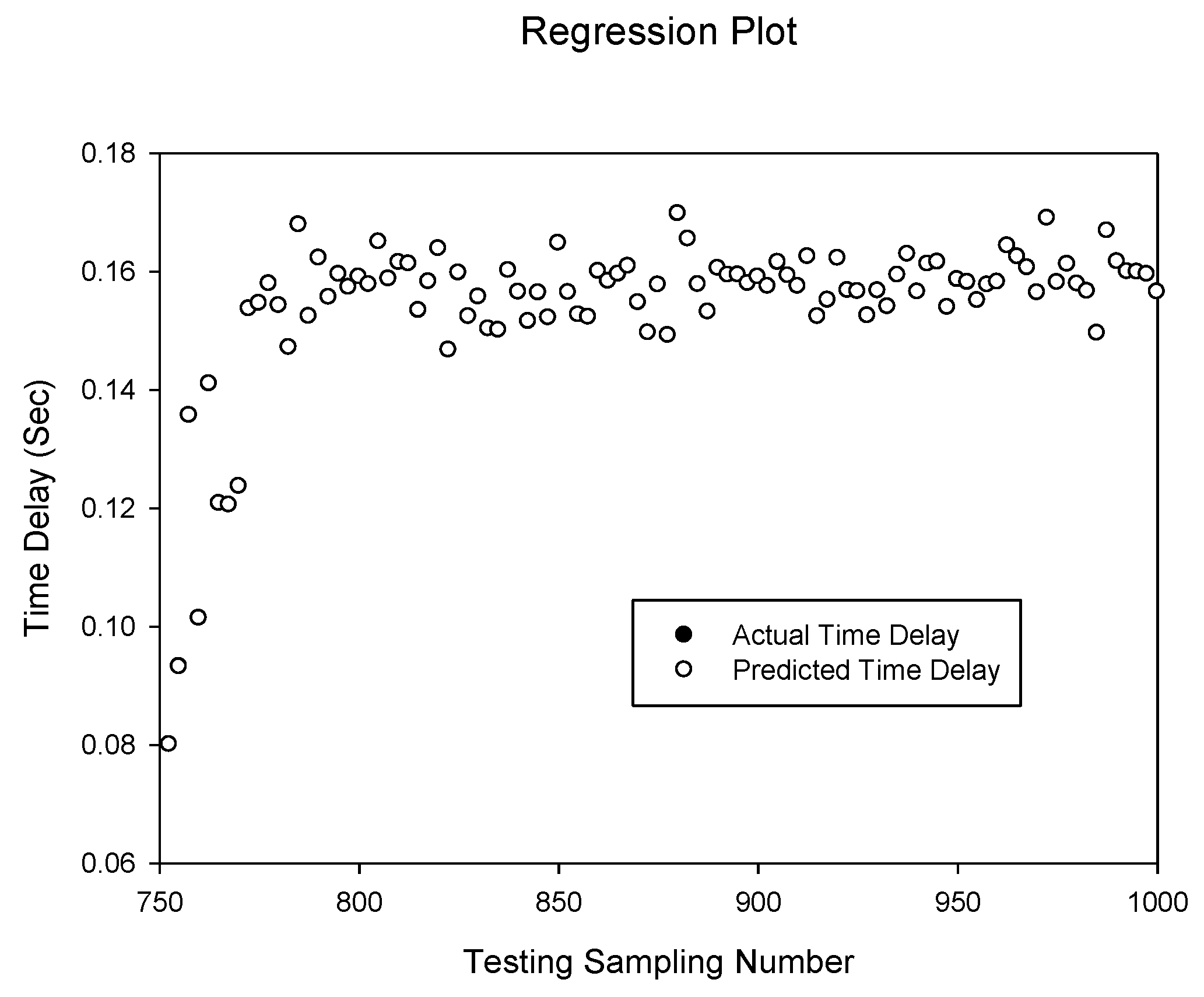
Figure 3.
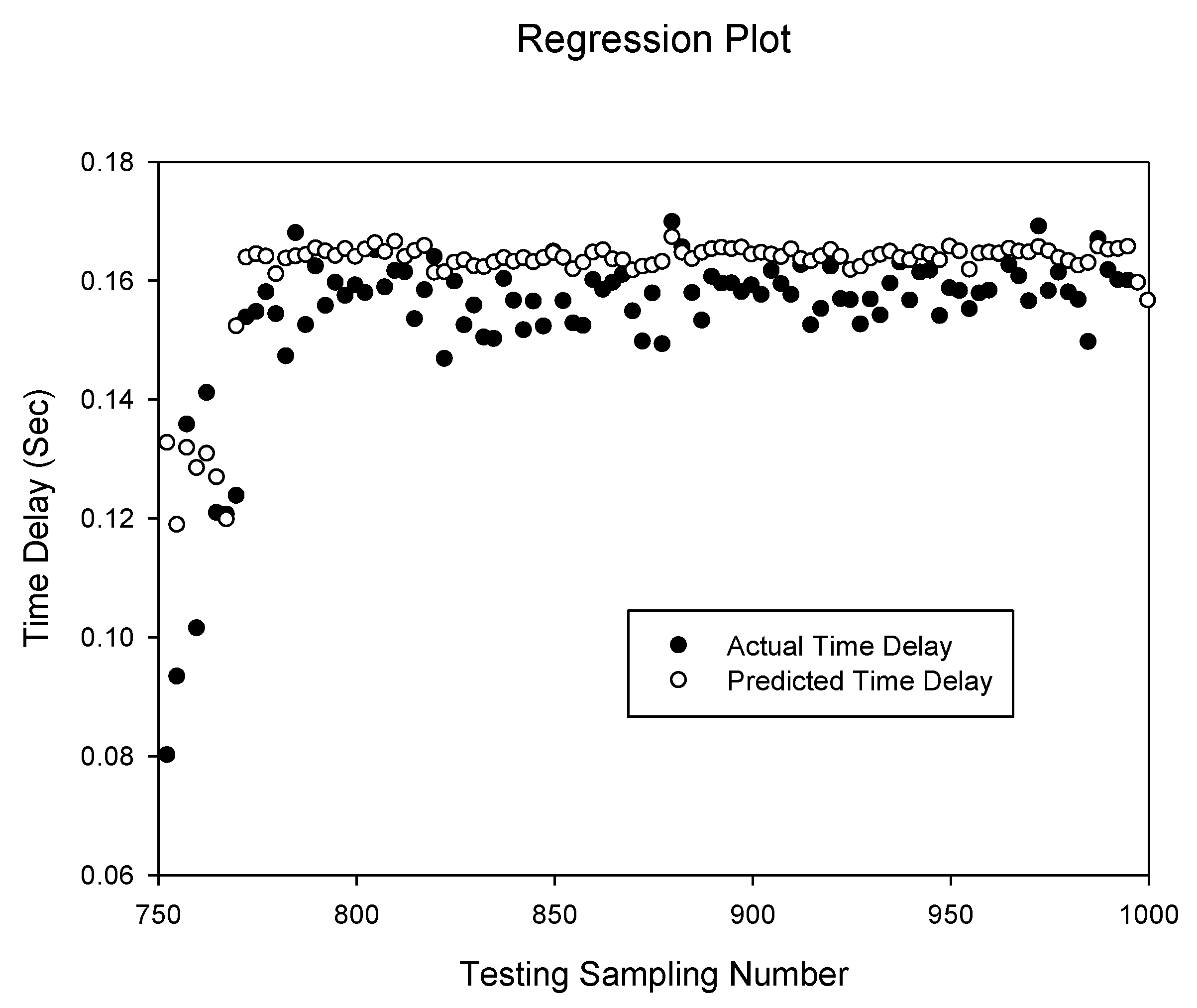
Prediction of delay sequence using BPNN(d)6,8.
Figure 3.
Prediction of delay sequence using BPNN(d)6,8.
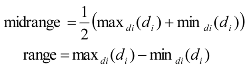
Figure 3 shows the prediction of the time delay sequences and gives a correlation of 0.999999999 by the
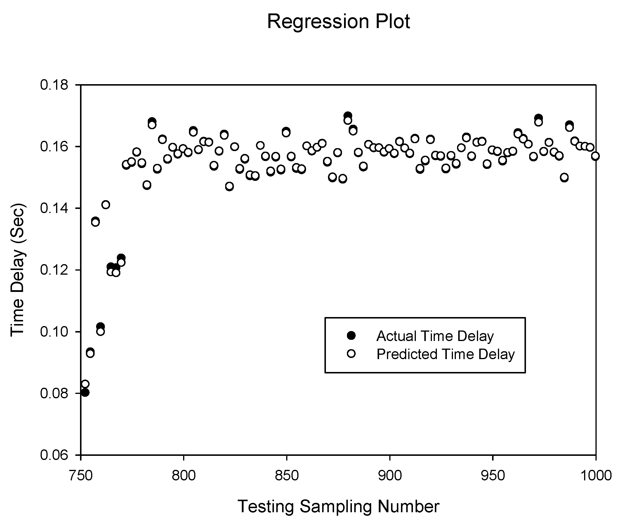
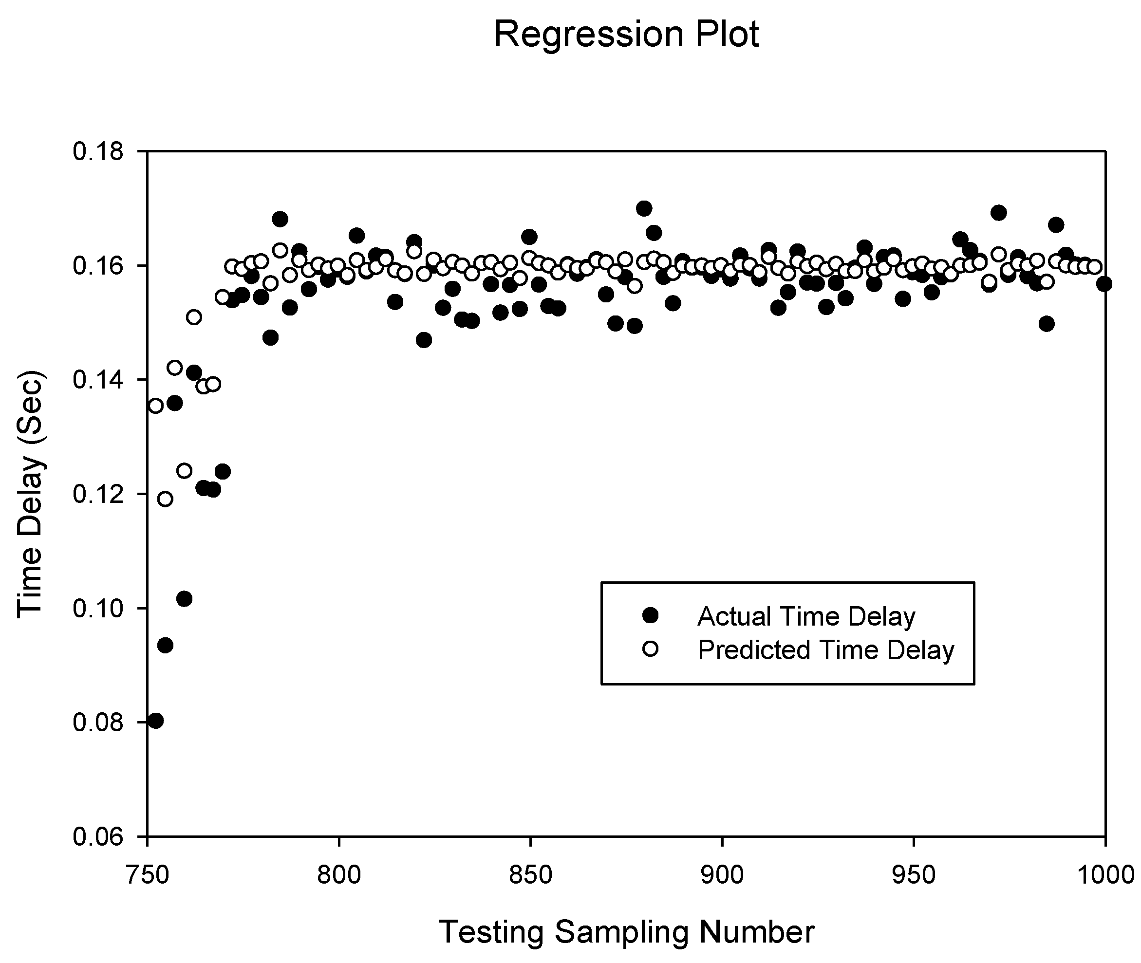
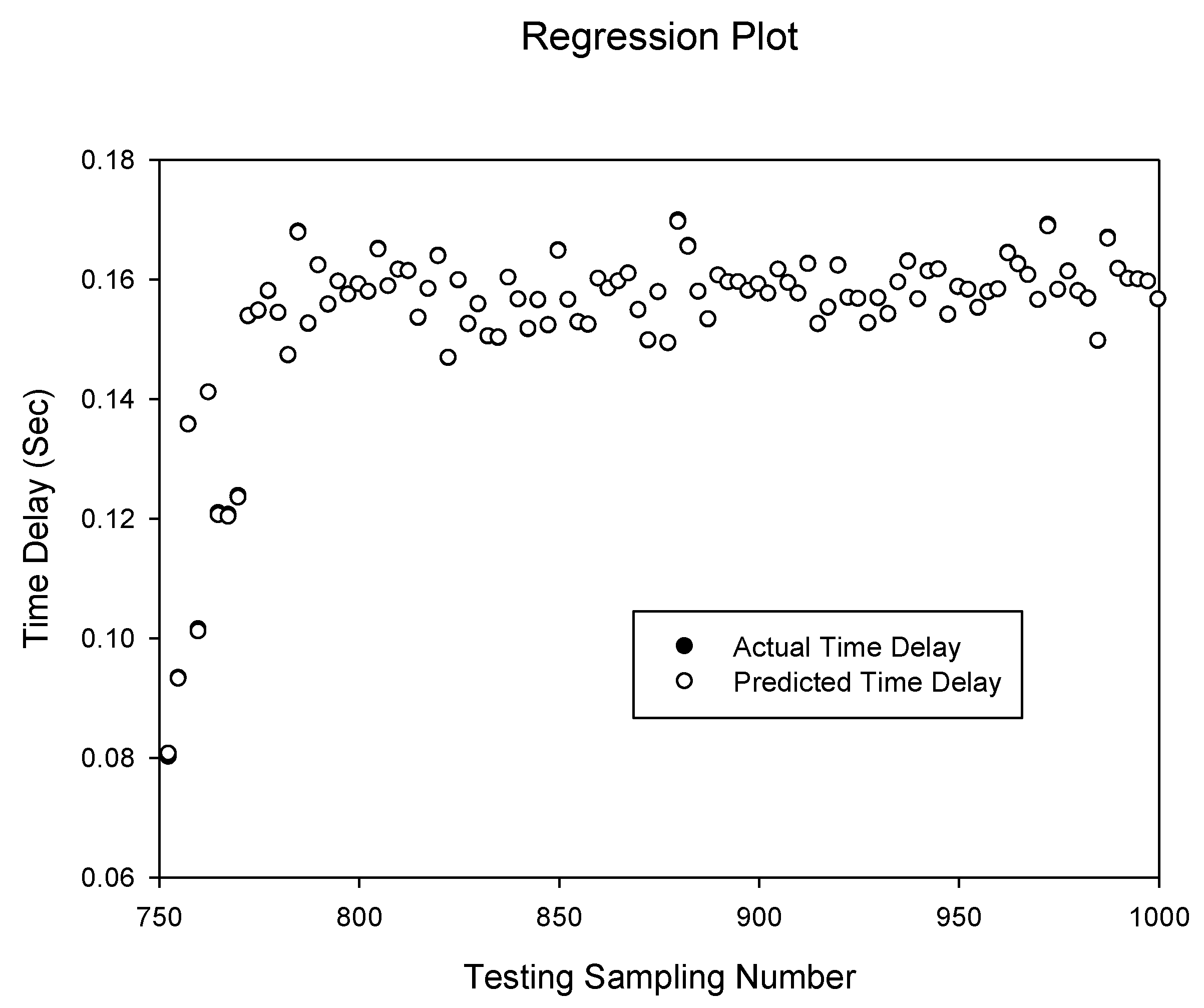
BPNN(d)6,8. It can be seen that prediction has a very high accuracy. The predicted values match the actual delay values. This high accuracy is also observed with the delay and network throughput combination as shown in
Figure 4 for the
BPNN(dt)6,8 network which has a correlation of 0.999996961. However, this is slightly lower than the
BPNN(d)6,8 network without the additional network throughput input.
Figure 4.
Prediction of delay sequence using BPNN(dt)6,8.
Figure 4.
Prediction of delay sequence using BPNN(dt)6,8.
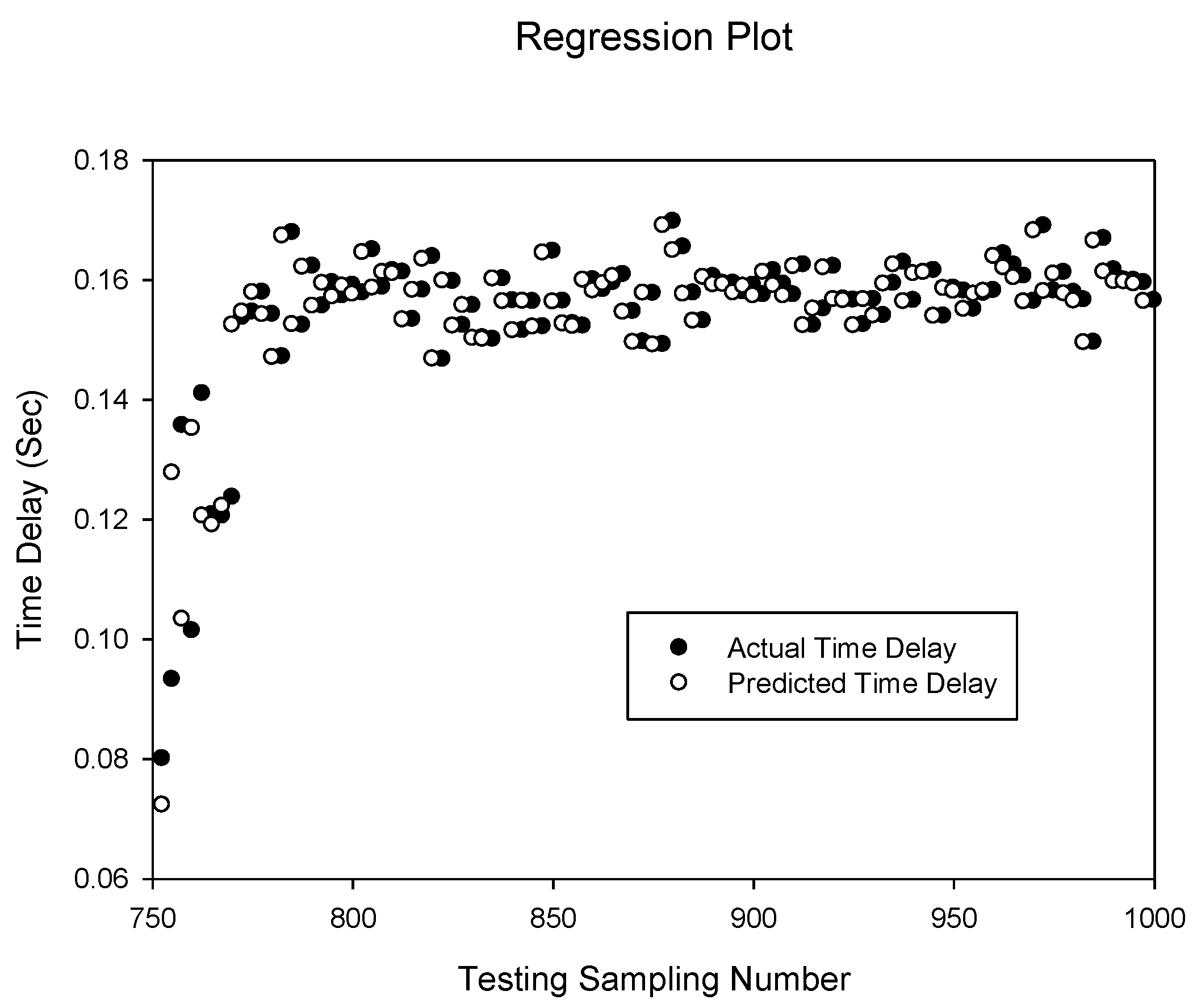
Figure 5 shows the prediction of the time delay sequence with correlation of 0.999999980 given by the
TDNN(d)8,5. It can be seen that the prediction accuracy is identical to the
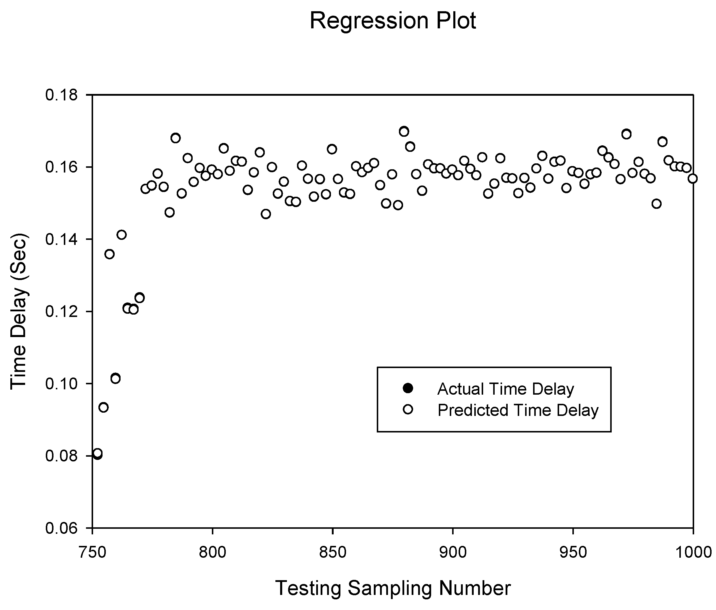
BPNN(d)6,8 topology predictions. However, the TDNN model requires a larger number of hidden neurons and more training iterations to achieve the same prediction accuracy. From
Figure 6, the
TDNN(dt)8,5 prediction accuracy is noticeably lower than the
TDNN(d)8,5. Compared to the previous two cases of the BPNN networks, the addition of the network throughput as an extra input is not significantly noticeable.
Figure 5.
Prediction of delay sequence using TDNN(d)8,5.
Figure 5.
Prediction of delay sequence using TDNN(d)8,5.
Figure 6.
Prediction of delay sequence using TDNN(dt)8,5.
Figure 6.
Prediction of delay sequence using TDNN(dt)8,5.
From
Figures 7 and
Figure 8 it can be seen that delay prediction using the NARXNN models lack adequate accuracy. The predicted values are around 10% deviation of the actual delay series. The prediction correlation for the delay
NARXNN(d)10,8 and
NARXNN(dt)10,8 delay plus network throughput combinations are 0.908709757 and 0.935523759 respectively. Interestingly, the delay plus throughput combination produces improved results in the NARXNN compared to the BPNN and TDNN models.
Figure 7.
Prediction of delay sequence using NARXNN(d)10,8.
Figure 7.
Prediction of delay sequence using NARXNN(d)10,8.
Figure 8.
Prediction of delay sequence using NARXNN(dt)10,8.
Figure 8.
Prediction of delay sequence using NARXNN(dt)10,8.
Figure 9 and
Figure 10 show the prediction of the delay sequence with correlation of 0.999997805 and 0.999999987 given by the
RBFNN(d)1,3 and
RBFNN(dt)1,3 respectively. It can be seen that the
RBFNN(dt)1,3 prediction accuracy is higher than the delay only input model
RBFNN(d)1,3 compared to the previous case of the NARXNN neural network model. Generally the RBF networks have a high correlation and simulations suggest that increased spread factor yields better results.
Figure 9.
Prediction of delay sequence using RBFNN(d)1,3.
Figure 9.
Prediction of delay sequence using RBFNN(d)1,3.
Figure 10.
Prediction of delay sequence using RBFNN(dt)1,3.
Figure 10.
Prediction of delay sequence using RBFNN(dt)1,3.
In summary, either the BPNNs, TDNN’s, RBFNN’s can achieve desired prediction accuracy for delay prediction in WSAN’s. The BPNN and TDNN networks needs more iterations (epochs) of training compared to an RBF network, while an RBF network needs more hidden neurons, i.e., the RBF networks required 17 hidden nodes which is double the size required compared to the BPNN and TDNN networks. This means that an RBF network is capable of faster learning compared to the BPNN and TDNN networks, but an RBF network needs more memory space for the network. The NARXNN network simulations did not yield acceptable results hence not used in our results comparison. As expected, the combination of the delay inputs with the network throughput inputs produced better results than the combination with the network packet loss rate. This shows that the network throughput is correlated with the delay experienced in wireless networks.
Comparing the results of the eight best sequences of the test results, we want to identify the best configuration capable of predicting delay sequences in wireless personal area networks for control applications. Based on these results, the appropriate topology for this is the topology with the best correlation and least network computing requirements which is the BPNN(d)6,8.
5.3. Inverted Pendulum Simulations
We integrate the proposed neural network to the control models and use the inverted pendulum on a cart system to test them to determine their effects and system response. The inverted pendulum is one of the most common systems used to test control system algorithms. Our simulations are done in the Matlab programming environment using the Simulink inverted pendulum simulation tool [
14]. We also assume that there is no packet loss in our experiments.
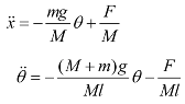
Without control, the inverted pendulum is unstable. To keep the inverted pendulum stable, a force F is applied to the cart to keep the pendulum in an upright position. The dynamics of the system are nonlinear. The coordinate of the cart’s position is denoted by x and the angular position of the pendulum denoted by θ. For this pendulum system, the control input is the force F that controls the cart in the horizontal plane. The system outputs are the angular position of the pendulum θ and the horizontal position of the cart x. The equation of motion used for the pendulum is determined by the constraints placed on its motion. The equations of motion for the pendulum can be thus described.
With the following notations:
x = cart position,
θ = pendulum angle,
F = applied force,
M = mass of cart,
m = mass of pendulum bob,
l = length of pendulum,
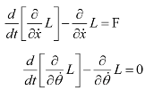
g = gravitational constant. The dynamics of the system can be derived from the Lagrange equations [
21].
where
L represents the Lagrangian function.
L = K −V where
K and
V are the kinetic and potential energies of the system respectively. The kinetic energy of the cart is defined as
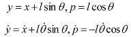
The kinetic energy of the pendulum bob is
where
p is the distance between the bob and the base of the cart
The total kinetic energy is defined as
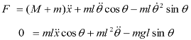
Substituting for
L in the lagrange equations and performing partial differentiation we have
Solving for
![Jsan 01 00299 i022]()
and
![Jsan 01 00299 i023]()
and performing linearization to obtain the linear state equations (the reader is referred to [
21] we have
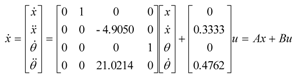
These equations yield the linear state space form
The output equation depends on the measurements to be taken. Our outputs are the cart position
x and angular position of the pendulum
θ. The output equation is then
Our inverted pendulum system parameters are listed below in
Table 7. We assume that the pendulum is linearized around the vertical position
i.e., it does not move more than few degrees.
Table 7.
Inverted pendulum parameters.
Table 7.
Inverted pendulum parameters.
| Mass of cart, M | 3 kg |
| Mass of pendulum bob, m | 1.5 kg |
| Length of pendulum, l | 0.7 metres |
| Gravitational constant, g | 9.81 |
Substituting the inverted pendulum system parameters defined in
Table 7 into the state space equation we have
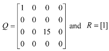
Looking at the eigen values of the system matrix A, we can verify the stability of the dynamic system. The calculated eigen values of A are [0, 0, 4.5849 −4.5849] and from this we can see that the system is unstable. We apply the linear quadratic control (LQR) methodology. The Q weights represent the different parts of the state. To weight the cart's position and the pendulums angle, the elements in the 1,1 position and 3,3 position is used respectively. The R matrix represents the input weighting. Since we are interested in maintaining the pendulum in an upright position, we drive the pendulum position state towards zero by inputting a larger entry in the corresponding part of the system state. After trial and error, we selected the weight matrices Q and R as:
The resultant desired state feedback gain K matrix used is [0.4023 −1.0747 72.3102 15.5374].
Variable Sampling Period
Consider the control system with delays using the same feedback gain and the observer based model. To simulate the networked circumstance, the neural network BPNN(d)6,8 predicted delay sequence is used which is the predicted value at sampling step k of the network induced delay one-step ahead. For the observer model, the system observer is sampled at every predicted total delay. First we investigate the case of variable sampling with the predicted delays by the NARXNN(d)10,8 as the sampling periods.
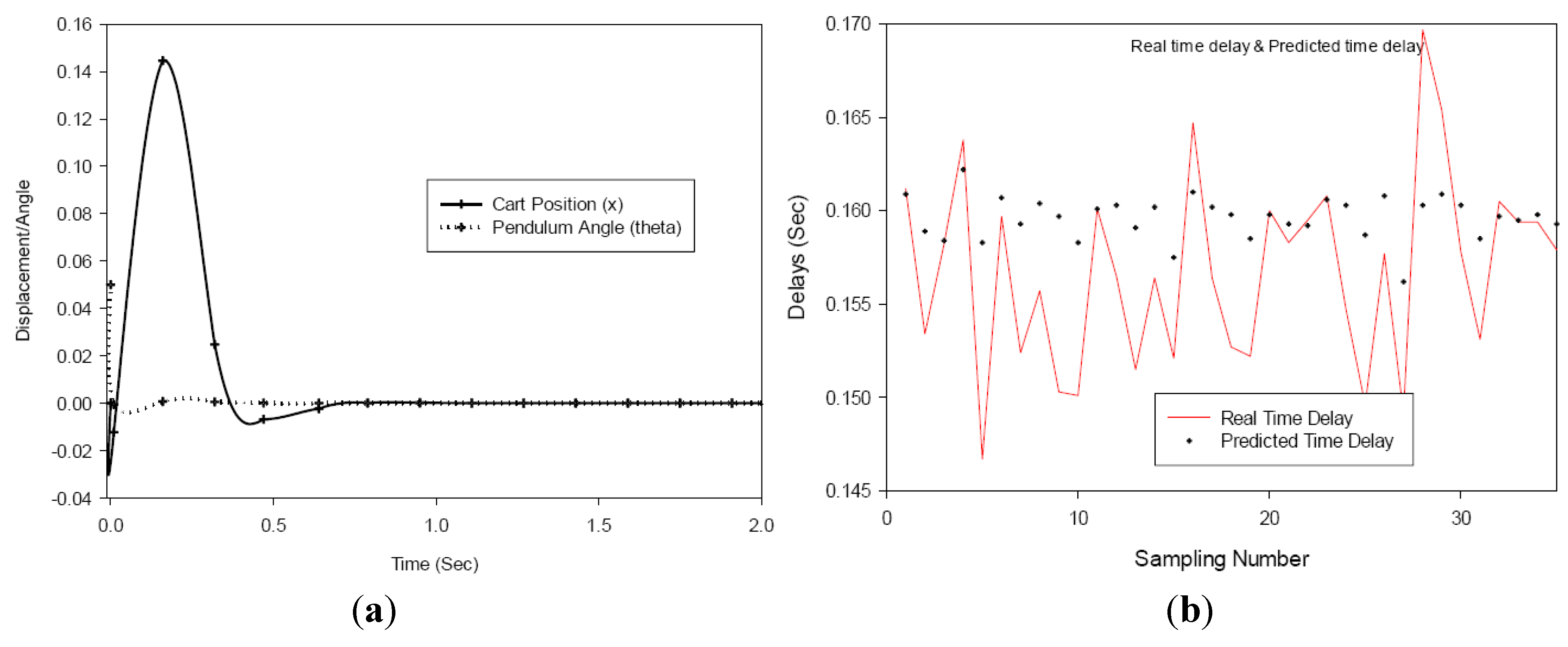
In
Figure 11 it shows that the pendulum converges to the goal about 0.804 s and the cart returns to its original position is 0.95 s with a maximum distance excursion of 0.16 to −0.01 m.
Figure 11.
(a) Variable sampling with inadequate delay prediction (b) Real vs. predicted time delay.
Figure 11.
(a) Variable sampling with inadequate delay prediction (b) Real vs. predicted time delay.
We also apply the BPNN(d)6,8 predicted delay values to the variable sampling observer. The initial position of the pendulum in the observer was set to θ = 0.05rad, same as the actual plant condition. After trial and error we set the observer gain to [−0.3 −0.31 −0.32 −0.33].
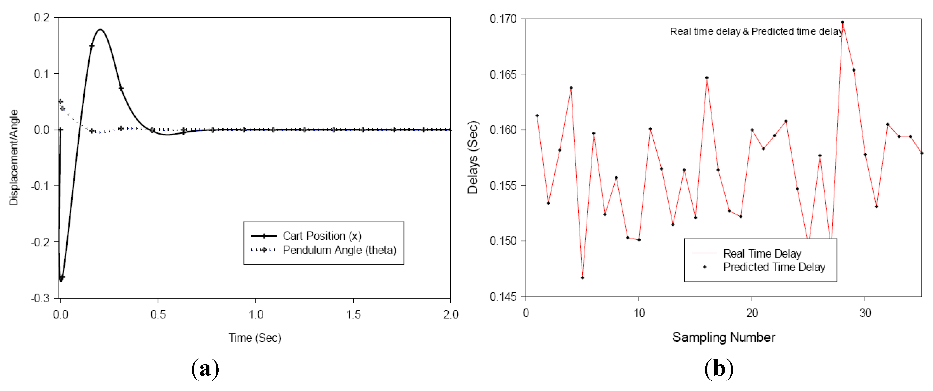
Figure 12.
(a) Variable sampling with adequate prediction (b) Real vs. predicted time delay.
Figure 12.
(a) Variable sampling with adequate prediction (b) Real vs. predicted time delay.
From the observer based variable sampling results in
Figure 12, the position of the pendulum is controlled adequately and the pendulum converges to its goal in about 0.64 s, with the maximum excursion of the cart 0.154 m and reaching steady state in 0.84 s. The results with the better predicted values by the
BPNN(d)6,8 produced better results than the
NARXNN(d)10,8 predicted delay values and points to the need for accurate prediction of the delays by the neural network.

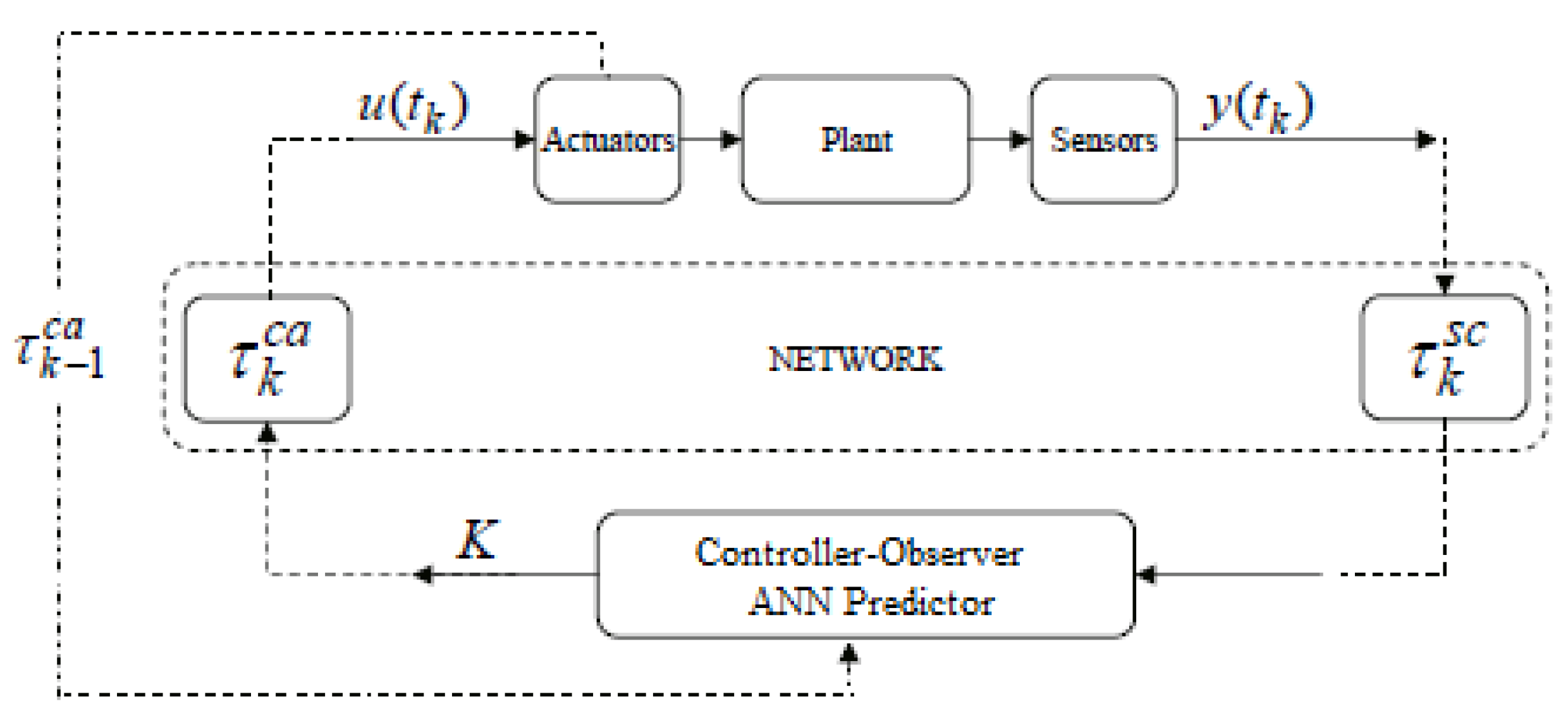
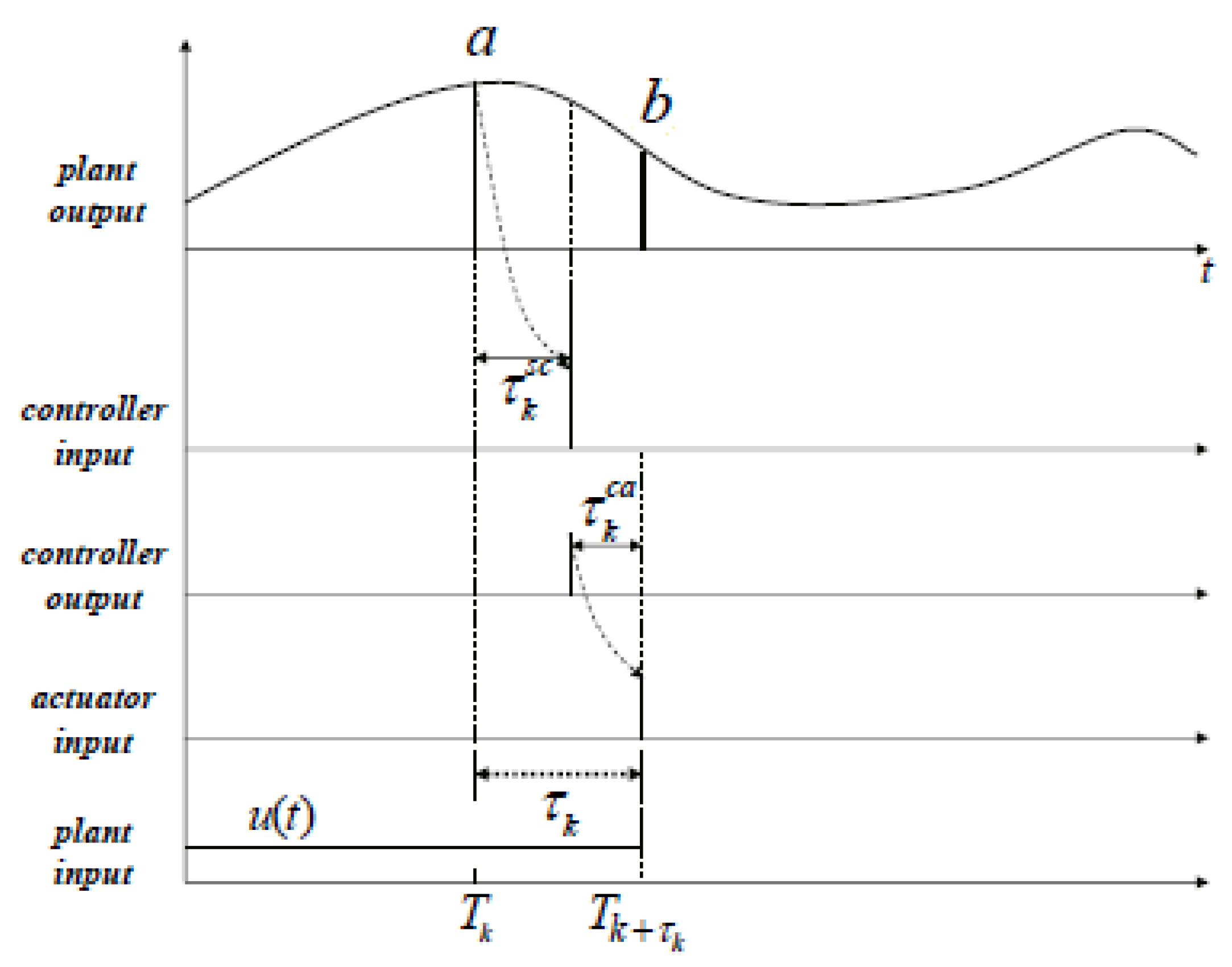
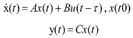

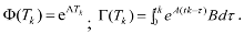
 represent the system states, the controlled input and output respectively. A, B and C are constant matrices of appropriate dimensions. K is the m × n feedback gain matrix. Here the system has variable sampling intervals, which implies that the system determines when the control signal is changed at sampling instant Tk. The total delay τk is assumed to be same as the sampling period Tk as it is expected that the ANN will precisely predict the future total delay τk [7]. The predicted delay τk = Tk, now becomes a parameter of the system matrix Φ and the input distribution matrix Γ. The discretized representation of the linear time-variant system with time-delay affecting the feedback is

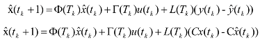
 , which will cause the estimated states
  to approach the values of the actual states x(tk). The prediction observers estimate the future plant states with differing sample times as predicted by the neural network. Control actions are calculated using the predicted states. Assuming u(tk) remains the same for tk ≤ t ≤ tk+1, the state x can be approximated by

 , where
  , the predicted state with observer becomes


 and
and  and performing linearization to obtain the linear state equations (the reader is referred to [21] we have