1. Introduction
Wireless Sensor Networks (WSNs) are envisioned to be flexible systems providing dense and cost-effective monitoring infrastructures. Their key features are absence of wires, long lifetime, and self-configuration, in spite of the limited resources. This has created enormous expectations around the technology, as an enabler of previously impossible scenarios as well as a credible replacement of established solutions. More than a decade of work has been carried out by the WSN community on this shared view, contributing to the promise of an easy-to-deploy functional instrument. However, while the complexity of handling this technology is well-known to computer scientists since the first experiences, the end user invests in WSNs to gather data from an obscure yet magic black box.
The state-of-the-art in WSNs presents a wide range of real world deployments mainly performed by computer scientists to satisfy end user requirements. Environmental monitoring in fire hazard areas [
1] has been one of the first use cases. In the Swiss alps, Beutel
et al. [
2] famously set up a system measuring the micro climate in high alpine regions. Werner-Allen
et al. [
3] made use of sensor networks to investigate active volcanoes. Structural health monitoring [
4,
5] and pipeline monitoring [
6] are further relevant examples. More related to our study, the SOSEWIN project [
7] represents a group of early warning systems using powerful hardware. With a similar focus, we [
8] previously worked on an early warning system for landslides.
Instead, we aim at describing a deployment experience from a different perspective, namely the one of a very interested end user with limited knowledge of the exact details of the technology. The end user works in the field of geotechnical engineering, where typical scenarios are ground subsidence, possibly caused by tunneling or mining operations, construction pit monitoring, and dam monitoring. WSNs have the potential to strongly improve traditional techniques, e.g., by providing real-time data to refine classical offline analyses and timely detect—possibly unforeseen—interactions between the ground and the surrounding buildings. Given the opportunity to access a concrete scenario to conduct experiments with the technology, he finds a company providing the hardware and the software, buys the equipment, and takes some people, more knowledgeable of WSNs, on board for the expedition. In this paper, we present such an expedition to deploy a WSN monitoring ground subsidence on a ground improvement site (
Section 3). For these purposes, we measured acceleration, inclination, temperature and barometric pressure using 21 sensor devices connected wirelessly to a fuel cell powered gateway forwarding the sensor data to a server via GSM (
Section 2). Here, following Langendoen
et al. [
9], our goal is to tell our unique story (
Section 4), the set of challenges we discovered day after day, due to both the harsh environment and the insufficient knowledge of the employed WSN hardware/software platform, as well as the solutions we put into action. The experience and the achieved data availability lay the foundation to look at the next steps (
Section 5) required to develop the much promised easy-to-deploy WSN black box.
While we do not focus on the domain specific results in this paper, the tilt, acceleration, and temperature data received from the network had the required quality. They allowed to monitor the stimulated subsidence in a previously unavailable time resolution. Joint analysis of the sensor data showed an interpretable spatial and temporal tilt vector distribution conforming to the geotechnical processes in the field.
2. Hardware and Software Design
For this application, we planned to use 20 sensor nodes (
Figure 1) and one gateway (
Figure 2) of the
Sensor-based Landslide Early Warning System (SLEWS) [
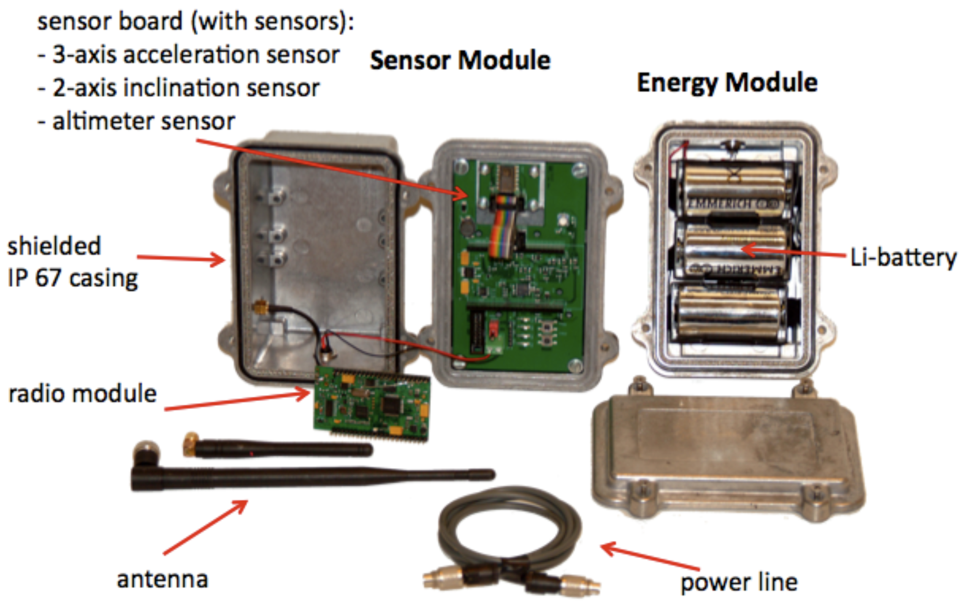
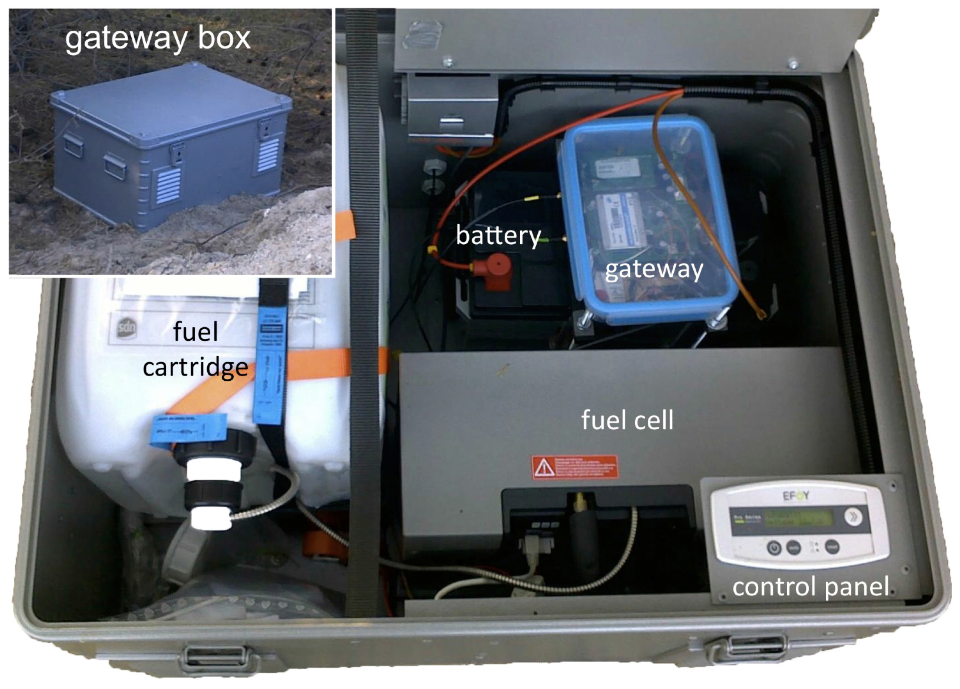
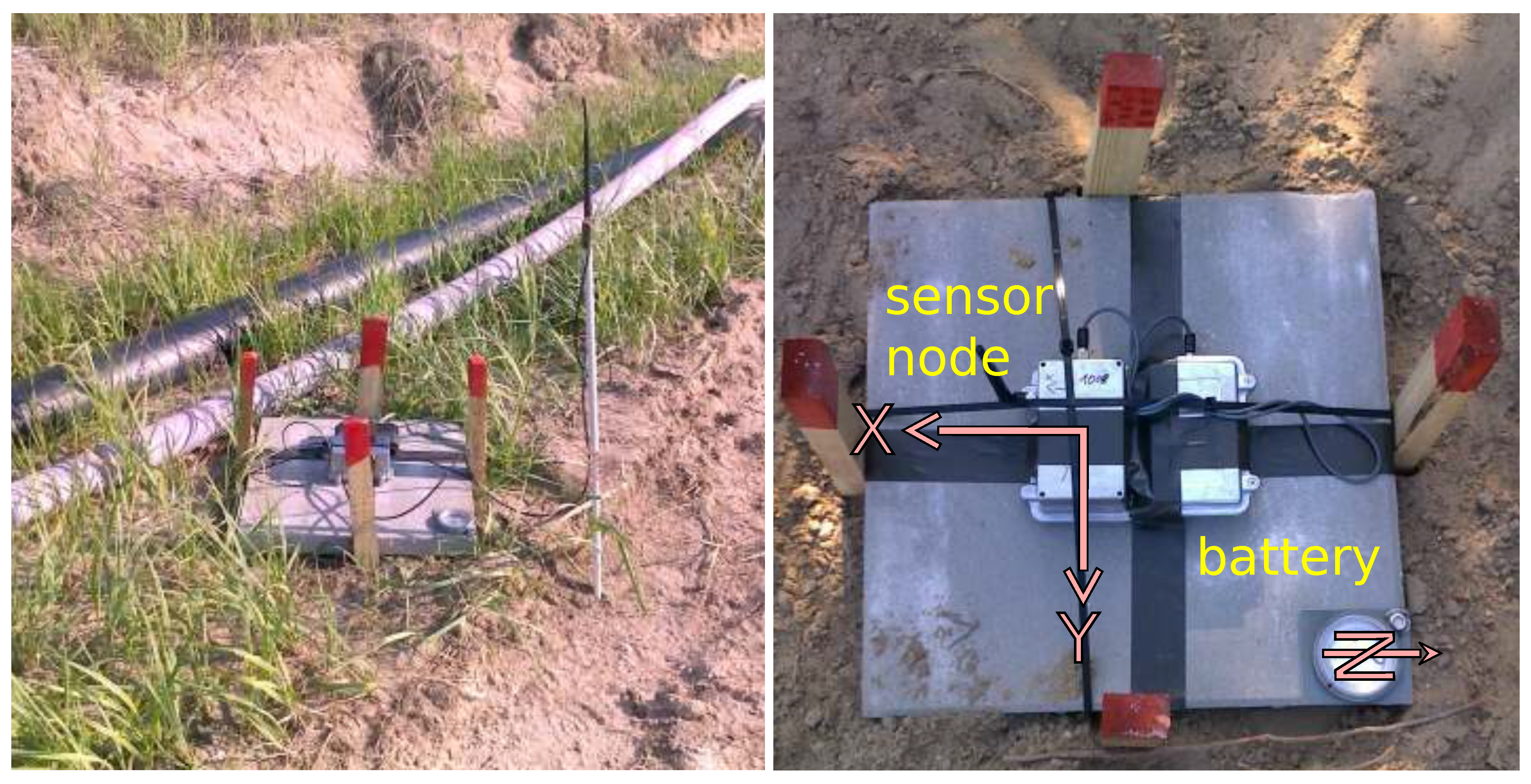
10]. We mounted the gateway to a fuel cell that recharged its 12 V/20 Ah battery if needed. For data transmission from the gateway to the server, we used the available GSM network. To protect the sensor nodes, we mounted them in shielded aluminum boxes with an ingress protection rating of 67. Three batteries, also in IP67 boxes, connected to the sensor nodes via cable to provide power supply (10.8 V, 5700 mAh). We used the CC1020 radio chip operating in the 868 MHz ISM frequency band for communication among sensors and gateway, achieving transmission distances of 10 m to 1.2 km with data rates from 4.8 kbit/s to 115 kbit/s, which we verified in earlier tests [
10].
Figure 1.
Sensor node, battery pack and components.
Figure 1.
Sensor node, battery pack and components.
The nodes consisted of a computation and communication core provided by ScatterWeb as a black box and a custom made sensor extension. The sensor extension included a 3-axis MEMS acceleration sensor (SPI interface, 1333 counts/g, ±2 g range, –40 ℃ to 125 ℃ operating temperature, 45 Hz bandwidth, 480
μA at 2.5 V), a 2-axis inclination sensor (SPI interface, 1638 counts/g, ±31° 8 Hz to 28 Hz bandwidth, –40 ℃ to 125 ℃ operating temperature, 4 mA at 5 V), and a barometric pressure sensor (SPI interface, 1.5 Pa/count, 30 kPa to 120 kPa range, −20 ℃ to 125 ℃ operating temperature, 4
μA at 2.7 V) [
8]. A separate voltage regulator for each sensor provided the necessary power. This allowed us to deactivate each sensor independently via the microcontroller (MSP430 by TI) running at 5 V. The supply circuit resides on the main sensor or gateway board.
For what concerns the software, we combined both the proprietary software, in particular for the sensor nodes and the gateway, and the more traditional tools for the services running on the server.
Figure 2.
Gateway with fuel cell.
Figure 2.
Gateway with fuel cell.
Sensor Node An external company had developed the software running on the sensor nodes. Its source code was available to us only a short time before the deployment. We did not discover the details of the network protocol until the deployment took place. The network protocol allows both receiving sensor data at the gateway via multiple hops as well as sending configuration commands to each sensor node. Such commands include enabling and disabling sensors, changing the sensing frequency and requesting the current configuration. For the test deployment, we had to mix up sensor node hardware from different batches that differed in small details on the sensor boards. Therefore, we did not reprogram all sensor nodes with the latest firmware but left several with their original firmware as shipped to us and apparently working. This lead to different versions of the firmware programmed on the sensor nodes.
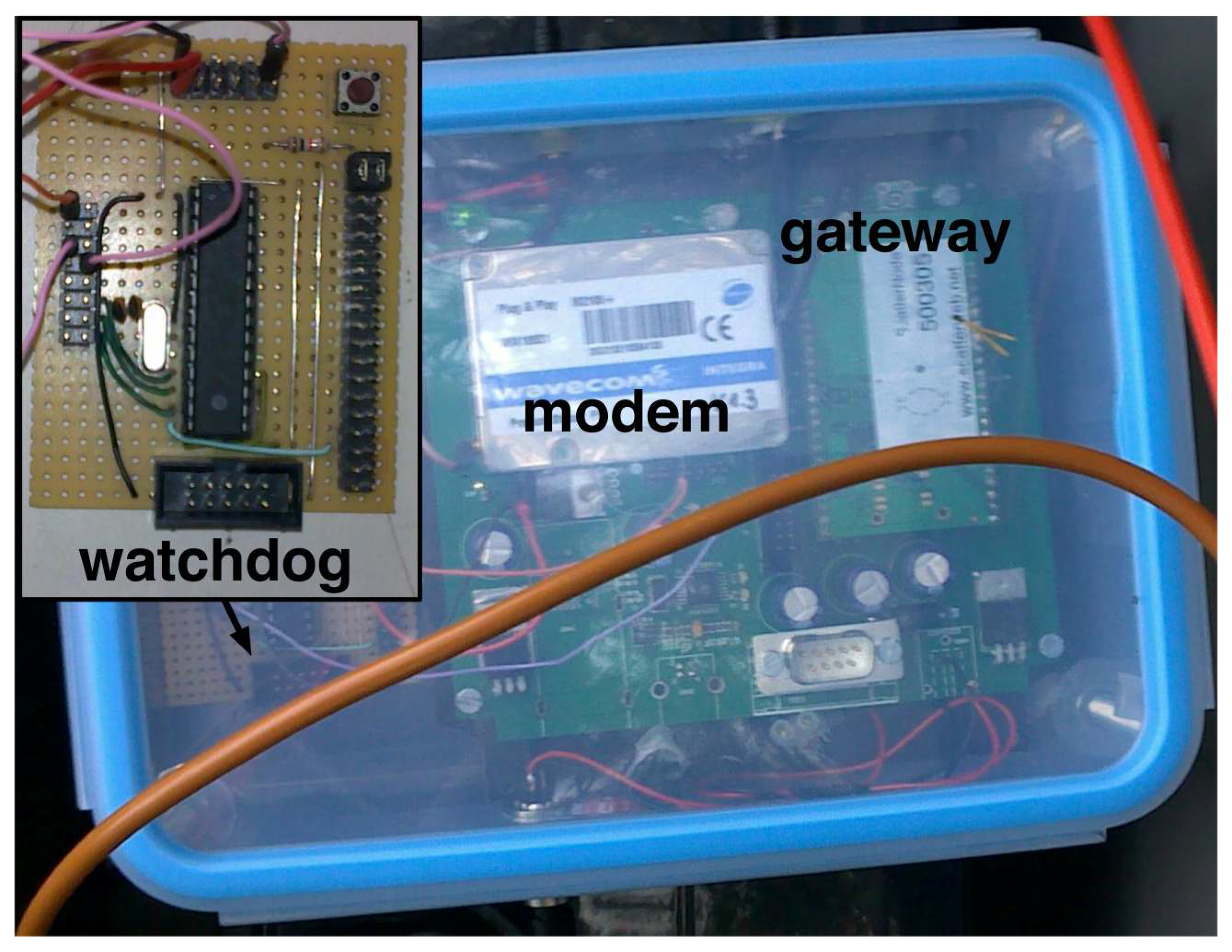
Gateway The same company developed the gateway, which provides only a link between the sensor network and a central server. To establish the connection to the server, the gateway is equipped with a GSM modem that opens a TCP connection via mobile Internet. In order to detect and re-establish broken connections, a keep-alive mechanism is implemented such that the gateway sends a PING to the server at regular intervals and, if a certain number of expected PONG responses by the server are missed, the gateway resets.
Server The gateway operates a GSM modem that opens a TCP connection to a server daemon. In our case the server was located at our university. The server daemon parses the data and stores the sensor values in a SQL database. It supports arbitrary many client connections and relays all data between all connected clients. With the data sent in human-readable format, we were able to use simple telnet connections to the server daemon for monitoring and debugging. Using standard UNIX tools like telnet, grep and screen, we built a flexible monitoring tool. For instance, if we wanted to identify nodes with bad radio connections, we filtered for the messages relating to sensor nodes joining or leaving the network. In order to accumulate different views on the data stream sent from the sensor network, multiple filters using grep and telnet were displayed simultaneously using screen. During deployment, we were able to quickly adapt such monitoring applications to the required scenarios without any programming effort.
3. Deployment Scenario
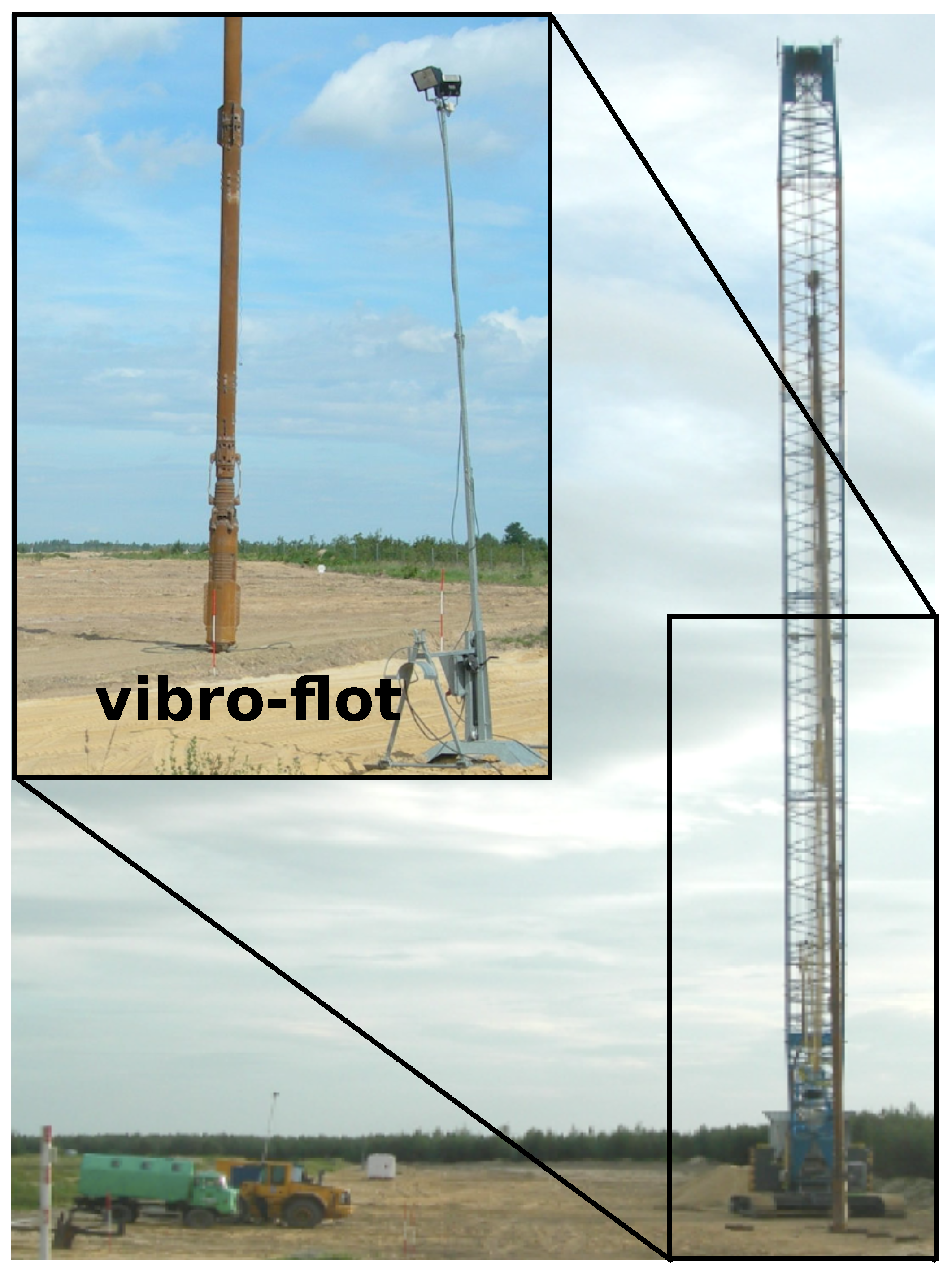
Monitoring of ground subsidence is an important task today, as ground subsidence causes considerable damages world-wide during tunneling, groundwater lowering, groundwater extraction, or mining operations. In the specific case of our study, a vibro-flot was used to perform ground improvement in a backfill area of a former open pit mine by dynamic compaction and monitored the resulting subsidence.
During a vibro-compaction campaign, a vibrating lance of 38 m height is immersed into the ground (see
Figure 3) and moves along a compaction track.
Figure 3.
Vibro-compactor.
Figure 3.
Vibro-compactor.
The vibration compacts the soil and reduces pore-space. Hence, the soil reaches a denser and therefore stable state. Subsidence due to the compaction of the soil results in a very slight, bowl-shaped depression that can be recognized only over a wide area. In addition, the presence of sizable machines, e.g., trucks, dumpers and vibro-compactors, as well as heavy-duty power and powerful electrical valves builds a challenging scenario for any monitoring infrastructure.
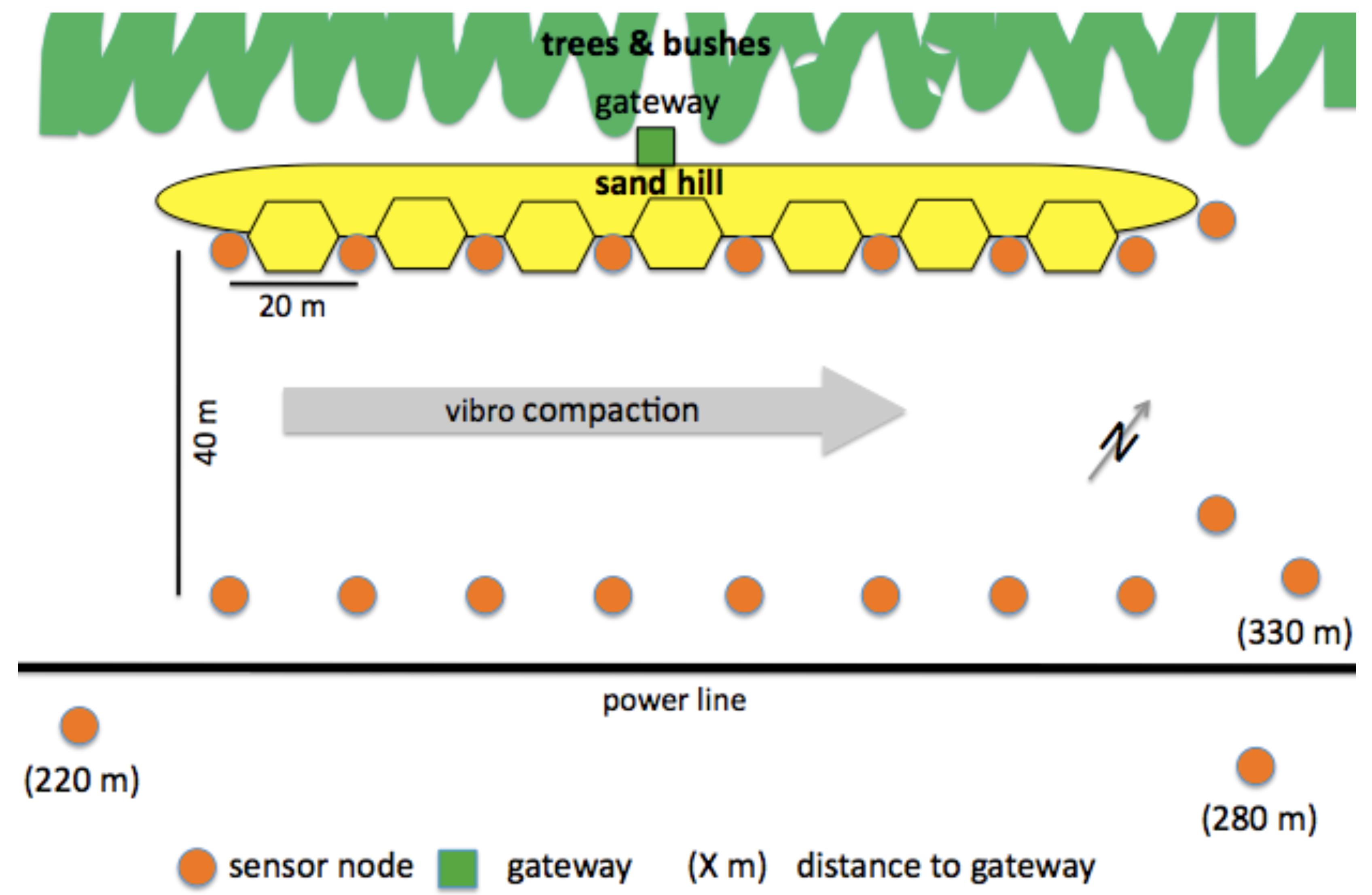
To monitor the progress of the compaction process, we deployed two rows of sensor devices at the sides of the 40 m wide compaction track, along the path followed by the vibro-compactor; in each row, nodes were deployed every 20 m. One row of nodes was surrounded on three sides by sand hills, leaving only the side facing the other row of nodes open. Finally, the gateway was installed behind sand hills in an area covered by trees and bushes to avoid that someone steals it.
Figure 4 depicts the resulting deployment map, as well as the location of power lines. As we describe in
Section 4, the deployment followed different stages, starting from a network composed of 12 sensor nodes, to which we added 6 new nodes in a second step. Moreover, we temporarily employed 3 additional nodes to perform communication range tests.
Figure 4.
Overview of the deployment. Sensor nodes, gateway, sandhills, power and water lines. Figure not to scale.
Figure 4.
Overview of the deployment. Sensor nodes, gateway, sandhills, power and water lines. Figure not to scale.
This placement enabled us to study the spatial and temporal propagation of the subsidence. Measurements show the change in inclination of the sensors as they tilt towards the center of subsidence over time. As the compaction campaign proceeds, it can be presumed that the change in inclination tends to point towards the vibro-flot. This scenario allows to observe ground subsidence in a controlled setting, although it is hard to measure absolute subsidence directly due to the complex mechanical behavior of sandy soils.
4. Time Line
Our deployment experience lasted, in the field, 37 days during the summer of 2011. In this section, we describe the several phases of the deployment, starting from the initial preparation in the laboratory, moving to the actual installation in the field, and concluding with additional ad-hoc tests we decided to run after observing the behavior of the system in operation.
4.1. Preparation in the Laboratory
In our former deployments, experiments with batteries and solar panels did not provide satisfactory results, as they could easily be affected by the specific weather conditions of the deployment. As a result, we decided to use an EFOY Pro 600 fuel cell, which performed very satisfactorily in preparatory tests, and therefore was implemented in the final deployment.
During the testing process, the gateway occasionally stopped working. The gateway was reaching an unknown state, from which it would recover only after an external reset. This event manifested in correspondence of the closure of the TCP connection between the gateway and the remote server, while trying to re-establish a connection. As the deployment area was more than 700 km away from our university, a manual reset was not an acceptable solution. Debugging the apparent problem in the gateway software handling the modem was impractical as it had been entirely developed by a third party.
One manifestation of the problem was the absence of communication between the microcontroller and the GSM modem. Therefore, we decided to install an external watchdog, as depicted in
Figure 5. This second, independent microcontroller (ATmega8) passively monitored the serial communication between the modem and the gateway microcontroller, and reset it through its external reset pin whenever no data was exchanged for 4 minutes. In addition, the board included two LEDs that indicated the proper operations of the watchdog and any previous forced reboot.
Figure 5.
External watchdog connected to the gateway board.
Figure 5.
External watchdog connected to the gateway board.
We tested each sensor node in the laboratory individually. Therefore, we assembled all the devices by combining the main board, holding the microcontroller and the radio chip, with the carrier board holding the sensors. During our initial tests, several of the nodes from the last batch were not able to join the network. With the help of serial debugging output and an additional LED, we realized that the faulty devices performed a reset when they would normally join the network. By swapping the sensor boards, we narrowed down the problem to a difference in the 3.3 V voltage regulators. We fixed this manufacturing problem by replacing the voltage regulators with others that supported a higher peak current. This enabled the malfunctioning nodes to join the network.
After this initial debugging, we tested all our sensors. We tested a maximum of 10 sensors at the time, always at distances smaller than 20 m. As we realized later, this was a mistake. In any case, confident in our equipment, we packed 16 sensor nodes, 16 battery packages, 2 gateways, 2 fuel cells, some spare parts, and our toolbox, and drove to the deployment site. Before leaving, we set up a second server to have the possibility for further testing if necessary. We believed that we had planned enough redundancy to be able to face any possible software and hardware failure.
4.2. Installation Phase at the Deployment Site
While traveling to the test site, we performed a last test of the processes running on the server at our university under high traffic load. This test was motivated by the delays amounting to several minutes that were experienced in the last lab experiments. First, we assumed a problem with the ability of the software daemon running on the server to handle massive data sent by the gateway. However, after intensively testing the service and temporarily replacing the TCP server with a simple Linux tool, it became clear that the problem was related to the mobile network provider. Apparently, the data sent from the gateway was cached for several minutes before being delivered to the server. In any case, the test of the server processes was successful, as we managed to accidentally fill up the whole disk space without encountering any problem.
The morning following our arrival, we went to the deployment site, which was closed for a few days for maintenance. The compaction track was prepared and all vegetation was removed. As shown in
Figure 4, in the sand wall deposited on the North-West side of the area, 9 notches were prepared to prevent the sensors from interfering with site operations. Then, we placed the concrete plates at their installation points (
Figure 6), on which we mounted the sensor nodes the following day. Finally, the gateway was positioned behind the sand wall, with antennas mounted at an elevated position, to ensure radio and GSM connectivity.
In order to test the sensors all in one place, we first prepared our sensor nodes outside the test field and connected them to their battery packs. Using a different gateway from the one already mounted to the fuel cell, we wanted to test all sensors at one location to save time before installing them at their final position. Via UMTS, we connected a notebook to our server and realized that we only received data from 9 out of 16 devices. At this point, we realized a first bug with our casing: the LED used for debugging was located inside the IP67 shielded casing and therefore not visible. Luckily, thanks to the sunny weather, we could open the cases. However, this operation took a considerable amount of time. We noticed that a break of the soldering joints at the connector for the power supply in 2 casings prevented those nodes from starting. After one hour and lots of cable checking we had 12 working sensors.
At this point, we activated the primary gateway and started the deployment. The first 4 deployed nodes associated directly with the gateway. However, the following 2 did not connect. In the end, we had 12 sensor nodes mounted on the concrete plates, of which only half appeared to be working properly. After 12 hours in the field, we went to the hotel frustrated.
In the last working hour, we discovered an additional problem. While the shielded casing protected our sensor nodes quite well, they also acted well as Faraday cages, caging electromagnetic waves. As we opened the casing of a node, which was not communicating with its neighbors, it directly joined the network. This revealed improper connection between the external antenna outside the casing and the radio chip inside the casing. With our former plastic casings this problem did not manifest itself, as radio waves could still propagate from the internal radio chip connectors. Following that, we started checking each node that was not joining the network and realized a number of faulty antenna connection. We took 6 faulty sensors from the deployment, repaired 2 while we were still in the field and took the others with us for the night shift. Fortunately, a construction site always provides enough energy for a soldering iron.
Figure 6.
Installation of sensor nodes.
Figure 6.
Installation of sensor nodes.
During the night, we repaired 2 of the faulty sensor nodes by replacing the antenna connections and flashing them with a new firmware. Two of the 6 sensors nodes could not be fixed, as one had a broken sensor board and the other had one of the wrong voltage regulators (see
Section 4.1), despite it having passed our tests in the laboratory. Highly motivated, we went back to the field. We installed the 4 repaired sensor nodes and rebooted the whole network. Only 8 of the 14 sensor nodes successfully started delivering data. Debugging started again.
We restarted the network several times and realized that some of the sensors were immediately connecting to the network while others were not. To improve connectivity, we placed the antennas of some of the sensors located in the niches at elevated positions. Despite this change, still, 4 sensors did not connect. By connecting them to a serial port, we seemingly verified them functioning. We further exchanged the position of several nodes, realizing that nodes that were not joining the network before started working properly. By chance, we then realized that several antennas seemed defective using a simple copper cable. So, we started looking for the working antennas. This process was quite hard, as some antenna seemed to work perfectly, some only when connected to specific nodes, and some not at all. Therefore, we started using colored flags to mark the behavior of each antenna. In some cases the PINs of the SMA connectors were defective, and in others the antenna cables were broken. After 3 hours, we identified 4 broken antennas and 2 working only at a short range.
At the end of the day, we had 14 sensor nodes working in the field, and we sent an order for new antennas and extensions to be shipped to the field. Moreover, we realized that 3G connectivity dropped significantly after 4 PM and reached at minimum at 6 PM. Having reached the goal of 12 operating sensors and 2 additional ones deployed in the field to test their performance, we left the field happy after long debugging days.
4.3. First Operation Phase—The Black Out
After leaving the deployment operational, we noticed the network topology was very unstable. Nodes were continuously changing their parent in the routing tree. At that time, we associated this behavior to the interference caused by the ongoing activities at the construction site.
And then, the weekend started. In the early morning of Saturday, two days after going online, we connected to the gateway on the test site. However, it seemed that no node was active at that time. The network routing table had only a single entry: the gateway. Over the course of the whole weekend, we could not see any improvement. All remote options like soft reset of the gateway or direct commands to single nodes did not improve the situation. On Monday, our partners working in the field tried to restart the nodes by switching the devices off and on again, again to no avail. Finally, on Monday afternoon we decided to give up, wait for some newly manufactured nodes, and travel as fast as possible to the deployment site.
On Tuesday afternoon, while discussing possible optimizations of the database handling traffic from more sensors, we realized that the (local) connection between the daemon running on the server and the local database was not active. The absence of any SQL transaction—all sensors had been absent for several days—caused a timeout of the connection. Unfortunately, no mechanism was in place to reestablish this connection, as this situation never happened during development and testing of the server processes. As soon as the connection was re-established, the routing table showed 9 sensor nodes connected and sending data. We had lost the connection between the gateway and our sensor nodes for at least 50 hours and suddenly they started sending data again. For the following week, 4 of them connected to the network only infrequently, and 5 worked seamlessly even in extreme weather conditions with thunderstorms, heavy precipitation and high temperatures.
Anyhow, monitoring the network connectivity and the traffic produced at the gateway, we realized that the network was rebooting quite often. High delays between the server and the gateway were causing the watchdog to reboot the gateway. Further analyzing this problem, it seemed that the gateway was rebooting particularly in the mornings and in the afternoons. As this problem seemed to be connected with the network connectivity, we decided to switch from our provider (1800 MHz, GPRS service) to another one (900 MHz, up to EDGE service). We also decided to allow the gateway watchdog a timeout of 8 minutes before rebooting the gateway, for the next phase of the deployment.
4.4. Second Operation Phase—New Sensors and Again Debugging
Fifteen days after the first deployment and 9 days after the network black-out, we went back to the construction site to extend the network to 20 nodes and investigate the reason why only 5 sensor nodes were delivering data. Due to heavy rain at our arrival, we could not open the casing of the nodes in the field. To save time, we added extensions to all working nodes so that the antennas were then at least 70 cm above the ground in a position with no or little shadow. Also, we rebooted all nodes not currently connected with a hard reset. Then, we replaced the gateway with our replacement using a SIM card from a different provider and updated the firmware with the new configuration for the watchdog. At the end of the day, 16 nodes were working correctly, with 6 of them new.
The following day, when the rain stopped, we started checking the remaining 7 sensors that were not working. We discovered 1 broken cable, 2 newly installed power cables where the poles have been swapped, and 2 faulty antenna connections. Due to the unstable weather, we decided to repair the equipment and further investigate the problems in our “field lab”. In our hotel, we realized that, surprisingly, 2 nodes had their network ID changed so that they were not recognized as part of the network. One of them, initially placed below a magnet valve, had to be replaced completely as it was malfunctioning and giving irreproducible results. Another node started working again after being reprogrammed.
We used the following 2 days to perform connectivity tests, which we describe in details in
Section 4.6, as well as to analyze GSM connectivity, and general network and gateway behavior. Also, we used this time to observe the compaction process, trying to correlate network dynamics and connectivity problems to construction operations. We observed that most working activities, e.g., compaction, dumping and rearranging of the construction site, corresponded to periods with increased occurrence of reconfigurations, which not necessarily involved loss of data. At the end of day 18, we still had 16 nodes working and 5 new nodes were ready for deployment.
We used the remaining 3 days in the field to deploy the remaining sensors and test the ability of the network to reconfigure in response to the ongoing activities at the site. Furthermore, we performed different experiments to investigate the performance and the limitations of the system for subsidence and ground movement monitoring, the initial aim of our deployment. At the end of the last day, we had 21 sensor nodes working in the field, 3 of them placed from 170 m to 250 m away from the rest of the network. Even at distances of 330 m, nodes could connect directly to the gateway. Moreover, we measured the time taken by the network to build a routing tree and start delivering data after being rebooted. On average, 35 min to 45 min were required to complete the setup process, with the majority of the nodes available after 20 min.
4.5. Data Availability—The Relevance of Up-Link Quality
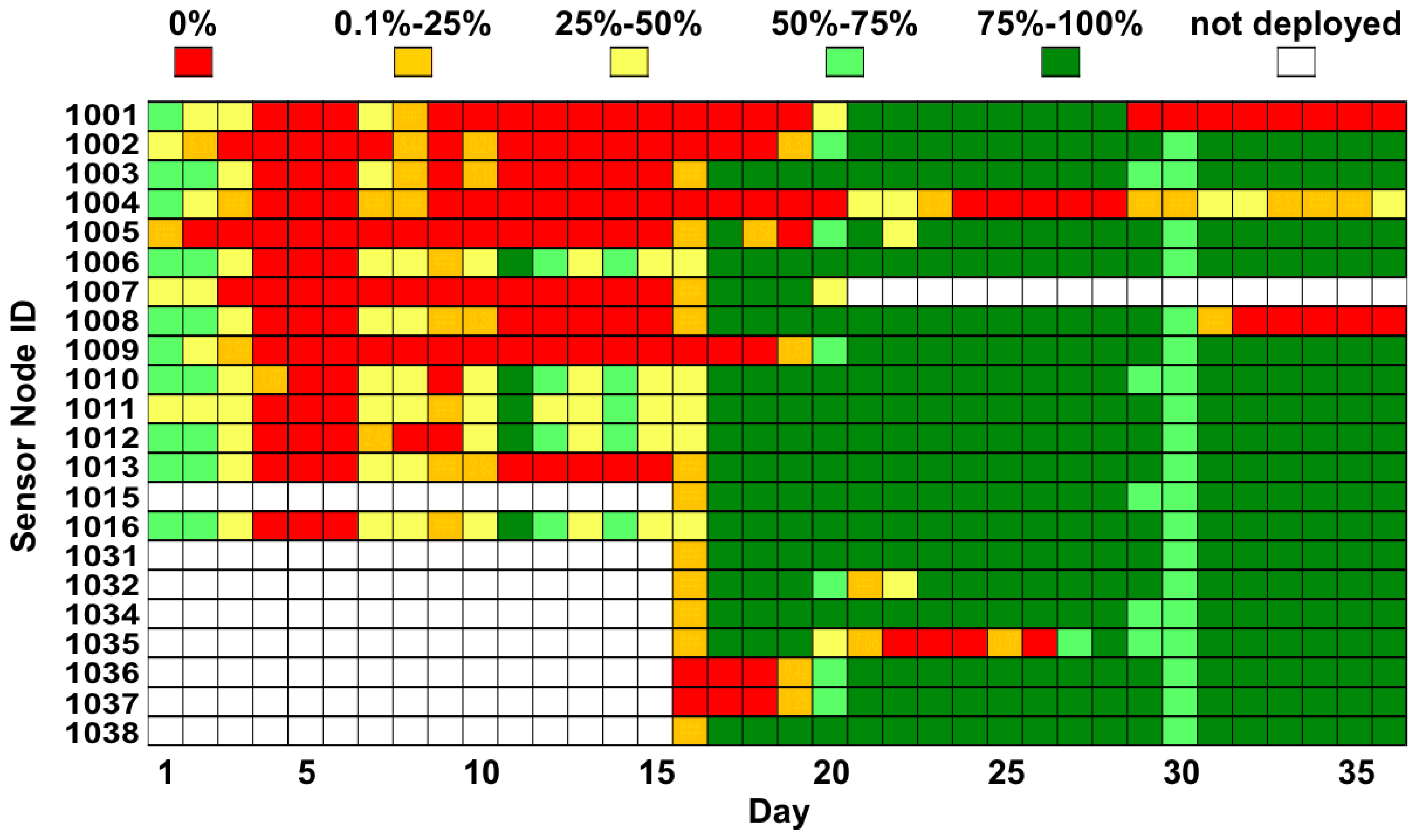
In
Figure 7, we computed the amount of data delivered to the server with respect to the configured sampling rate of each device. It is possible to clearly distinguish the discontinuity in the first two weeks of operation, followed by the higher availability of data, later.
This clear change corresponds to the change of the 2G provider. This becomes even more evident by looking at the actual percentage of delivered samples. In the first deployment phase, the amount of delivered data only rarely reached more than 50%. In the second phase of the deployment, the new system configuration significantly improved the overall performance. This confirms the absolute importance of the reliability of the data up-link on the perceived overall performance for the end user. On the 30th day, the IT department performed maintenance work on our server, as they expected our deployment to be completed already. As our services did not start automatically on server boot, we lost the data until—by chance—we realized that none of our processes were active.
Figure 7.
Percentage of data successfully Delivered to the remote server.
Figure 7.
Percentage of data successfully Delivered to the remote server.
4.6. Range Tests and Connectivity Tests—It Is Not Always the Hardware
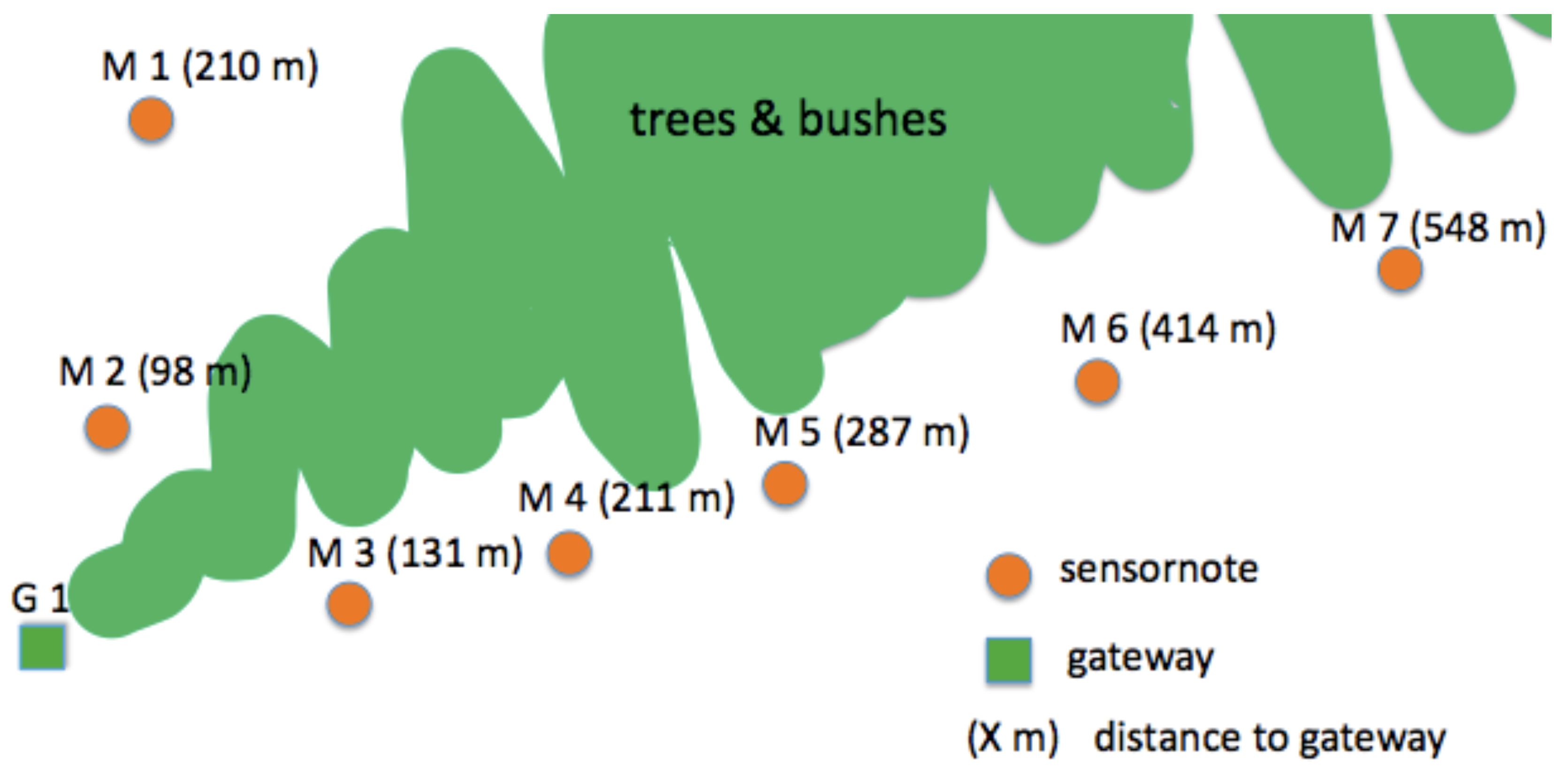
Due to the connectivity problems experienced in the first deployment phase, we executed some range experiment with 5 nodes. For these tests, we used nodes that had previously shown connectivity issues. After checking the antenna connection and cables, as well as reprogramming them, we could assess their functioning individually. Apart from hardware problems of one node that we had to discard, the nodes worked properly from the very beginning.
To avoid interference with the operational network, we used a second gateway and an independent remote server. The sensors were placed next to a road track along two lines, in the configuration shown in
Figure 8. The two lines of sensors were divided by an area covered by bushes and trees. We placed the gateway at the junction of the two lines in the shadow of a large tree. To enhance connectivity, the antenna was placed on a 2.5 m pile.
Initially, the sensors were placed at ranges of about 50 m around the gateway, while the network topology was monitored. Once all the nodes were connected, we moved them so to cover distances between 100 m and 550 m. In the first tests, we made use of hard resets to investigate routing setup times. It took about 6 minutes for the first sensor to start transmitting data, and the rest of the network became available within 8 min to 35 min. Surprisingly, these times were independent of the distance of the notes to the gateway.
Figure 8.
Deployment for range test.
Figure 8.
Deployment for range test.
Independent of their position, most sensors connected directly to the gateway, even if bushes and trees were in the line of sight. In the case of multi-hop routing paths, nodes predominantly chose long distance links. In one specific case, a node placed between two connected sensors was not able to join the network. Our debugging tools did not indicate any malfunctioning. After restarting the whole network, this node started working again, even at a distance of more than 550 m from the gateway.
Before leaving the deployment area, we decided to take the chance to perform a final test overnight to investigate general connectivity and data routing. After having collected all our equipment, we went to a grassland next to the construction site, where we deployed all our 26 sensor nodes at pseudo-random locations. As a general rule, we tried to place devices at least at 50 m from each other, at the maximum distance of 960 m from the gateway. The sensor nodes were placed directly on the ground, with the antenna at about 70 cm height.
During the experiments, the number of nodes able to deliver data at each time greatly varied. Interestingly, at no point was it possible for all the devices to connect to the network at the same time. By monitoring the evolution of the network, we could clearly identify alternating periods with 12 to 15 nodes connected, followed by periods with only 4 to 6 nodes available. Surprisingly, the routing tree would often have a maximum depth of 7 hops. Unfortunately, the result was more of an oscillating connectivity than the desired opportunistic distribution of data loads exploiting the dynamics of the communication patterns.
While certain nodes worked well in one particular orientation and location, they did not connect at all in a different surrounding and environment, even though their hardware and software was verified to be working. This difference in behavior is not yet addressed adequately in the literature. We need protocols and methodologies to help a non-expert user to trouble-shoot this behavior at deployment time, which cannot be addressed by the sensor network hardware and software alone.
5. Conclusions: Lessons Learned
After our experience, we discuss the major lessons we learned, keeping the end user as the reference for our future efforts. Despite some of the findings are not necessarily new to the community, we firmly believe in the importance of keeping the debate open.
What makes a WSN? At the end of the day, a WSN is nothing more than a monitoring (maybe controlling) instrument. As such, the most relevant metric for the end user is the amount of data permanently accessible and their accuracy. While the latter find very little room in deployment reports (as admittedly in this paper, too), the former often accounts for the messages only reaching the gateway, as if that was the end point of the system. In the experience we reported, a non-negligible amount of data was lost after reaching the sink due to problems on the gateway, on the link to the data server, or on the data server itself. While we often see expected lifetime as a driving evaluation metric, we think that the concrete data delivered to the user should be the defining factor of a successful data collection system. As a result, proper tools should be designed to reliably move data from the single sensor to the final storage location, along the entire delivery chain, enabling diagnosis of failures up to the very last mile of the system. Accordingly, for event-based warning or control systems, we need to consider the end-to-end delay and on-line availability along this chain.
Communication is the enabler. Despite the efforts in defining more and more complex communication models, the unpredictability of wireless propagation in the field due to physical obstacles or hardware imperfections is a common experience. Unfortunately, prior experience, even in the same scenario, can be of little help; small changes in the node placement can completely change the network topology. However, communication does not only enable the functioning of the application, but also the debugging of the system itself. Even if the characteristics of wireless links cannot be predicted, they can certainly be studied systematically in the field. Keeping as reference the locations where the end user plans to monitor the quantity of interest, methods need to be designed to indicate where to install additional devices necessary to ensure general connectivity.
The user can do more than rebooting and replacing batteries. The complexity of building WSNs often comes together with the presumption that only experts can debug it. In our experience, we realized that even the non-expert end user provides incredible debugging support when equipped with proper tools and pointed in the right directions. Not surprisingly, he is often present and available in the deployment field and already equipped, e.g., in the form of smartphones. Nonetheless, we keep relying on obscure LED blinking schemes and wizardry computed on textual log files to make a diagnosis of problems; this debugging technique is, indeed, annoying and inconvenient also for experts. Expressive interfaces should be part of the system design, since the very beginning. Similarly, effort should be made to aggregate low level information, understandable only to experts, in high level instructions to enable the end user to perform first exploration of the problems.
If the field were like a lab. We tend to consider deployment in the field as yet another experimental setting, where to continue the “trial and error” techniques typical of the laboratory. Different configurations are tested with a rule of thumb until the first working one is found. This method is simply unacceptable when installing an operational system, not to say inefficient. Definitions of proper deployment methodologies are needed, also to identify the specific tools required to make the overall process easier. After a first exhaustive local diagnosis of each system component, knowledge about the environment and how it characterizes system properties should be acquired. Such information, together with application requirements, should be used as input to provide feasible system configurations. The system should then be incrementally deployed and tested against the application constraints so that problems and involved components can be detected effectively. The end user is willing to provide support but for lack of experience needs proper guidelines with defined rules and strategies. Finally, problem detection and diagnosis should be an integral part of the running services for the entire system lifetime.
In many cases, WSNs leave the impression to the possible end users that they are still nice toys made for the pleasure of computer scientists. When the opportunity for a real application rises, WSNs are still deployed according to the rule of laboratory experimentation. The development of systematic methodologies to guide the different steps of a typical deployment, as well as the tools required to implement them, is crucial to transform the technology in an actual product. To cover this gap, we necessarily need to take the perspective of the end user as reference, to make these systems wide-spread and manageable by non-experts.

 ,
, 