Performance of Cooperative Eigenvalue Spectrum Sensing with a Realistic Receiver Model under Impulsive Noise


Abstract
:
1. Introduction
1.1. The Realistic Implementation-Oriented Model
1.2. Eigenvalue-based Sensing Schemes
1.3. Impulsive Noise
1.4. Our Contribution
2. Model
2.1. Centralized Eigenvalue-based Spectrum Sensing


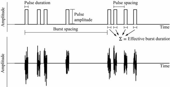
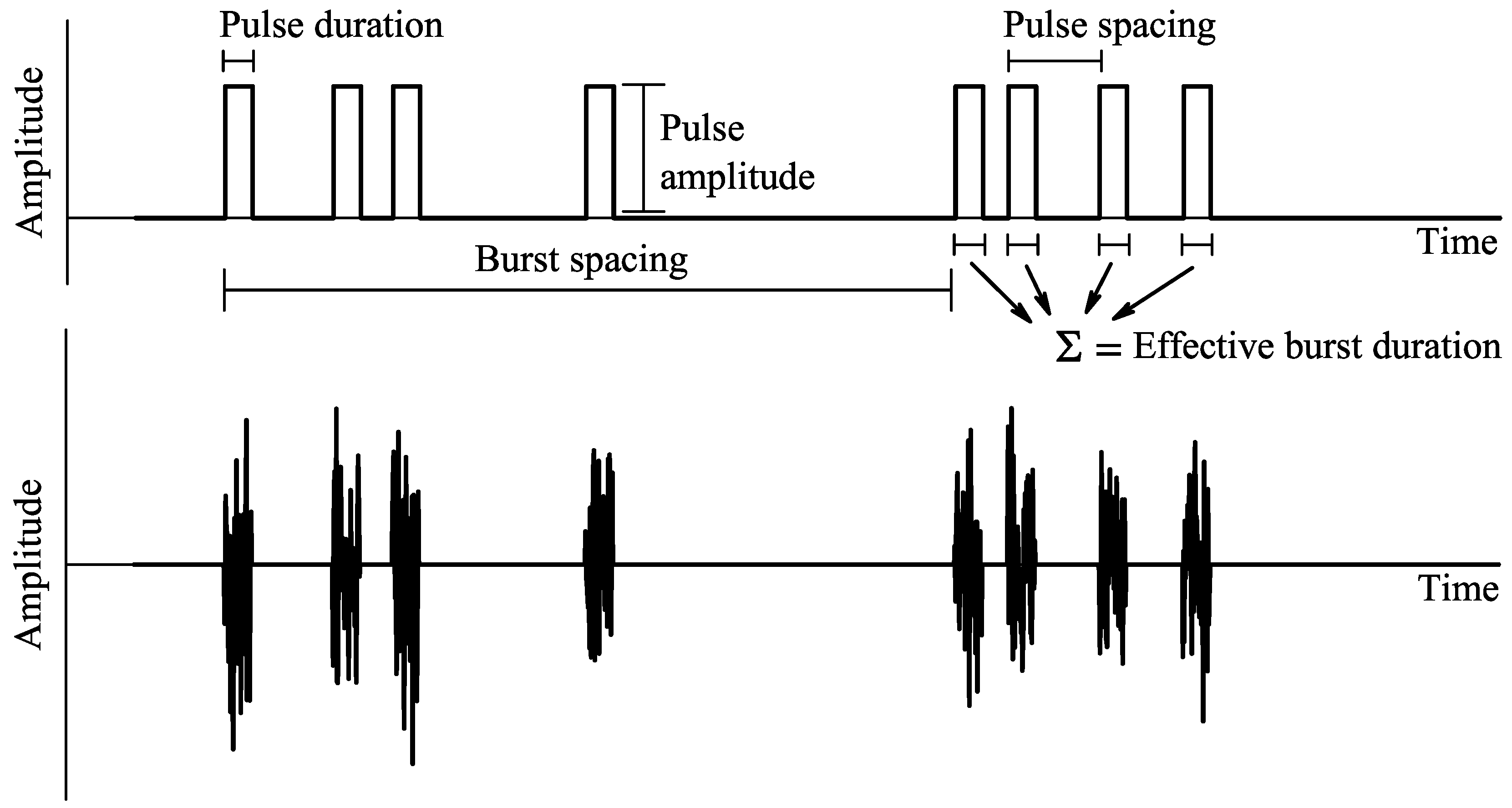
2.2. IN Model

3. Simulation Setup
3.1. Conventional Model (C-Model)
 .
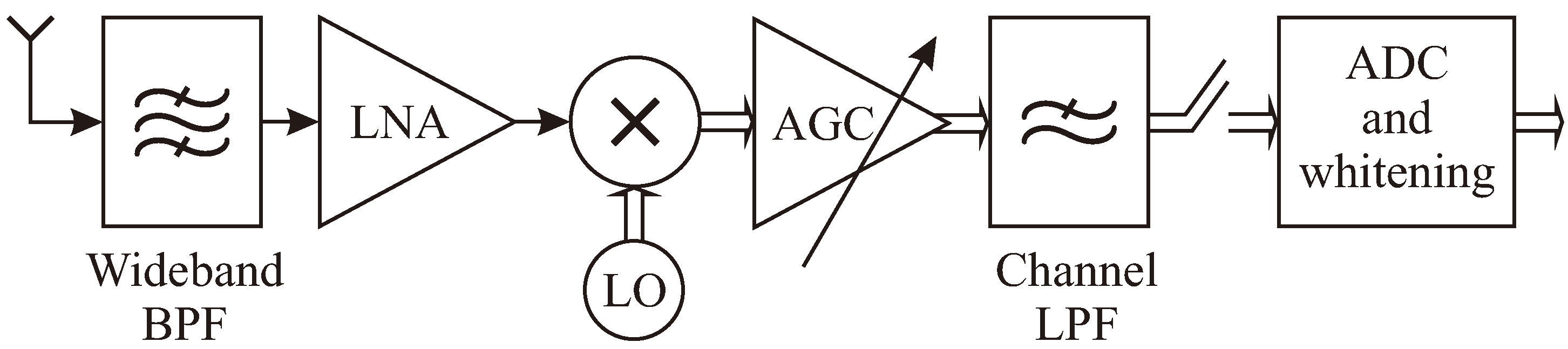
. 3.2. Implementation-Oriented Model (R-Model)
 for unitary average received signal power,
  for an SNR-dependent average thermal noise power, and
  for an average IN power K times the thermal noise power, where the symbol “←” represents the normalization process, PX, PV, and PVIN are the average time-series powers in X, V, and VIN before normalization, respectively. Moreover, to guarantee the desired received SNR, matrix H is normalized so that .
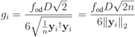
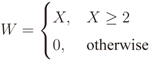
 , which means that the signal power at the output of the AGC will be σ2 = 2D2/36. This justifies the factor
  in Equation (7). Finally, as the name indicates, the overdrive factor fod ≥ is included as a multiplier in Equation (7) to simulate different levels of signal clipping caused by real ADCs, i.e., it produces signal amplitudes greater than or equal to 6 . For example, an fod = 1.2 means that the dynamic ranges of the signals at the input of the I&Q ADCs will be 20% larger than the dynamic ranges of the ADC’s inputs. The I&Q clippings act on each sample value s applied to their inputs according to s ← sign(s)min(|s|, D/2).
 4. Influence of the System Parameters

| C-Model and R-Model | |
| Signal-to-noise ratio | SNR = −10 dB |
| Number of primary transmitters | p = 1 |
| Number of CRs | m = 6 |
| Number of samples collected by each CR | n = 50, 100 |
| Impulsive to thermal noise power ratio | K = 0 |
| Signal-to-noise ratio | SNR = −10 |
| MA-filter length | L = 1-20 |
| ADC dynamic range | D = 2 |
| ADC overdrive factor | fod = 1-2 |
| Number of quantization levels | Nq = 4, 8, 256 |
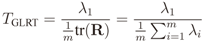
4.1. GLRT
4.2. MMED (or ERD)
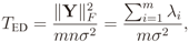
4.3. MED (or RLRT) and ED

5. Influence of IN
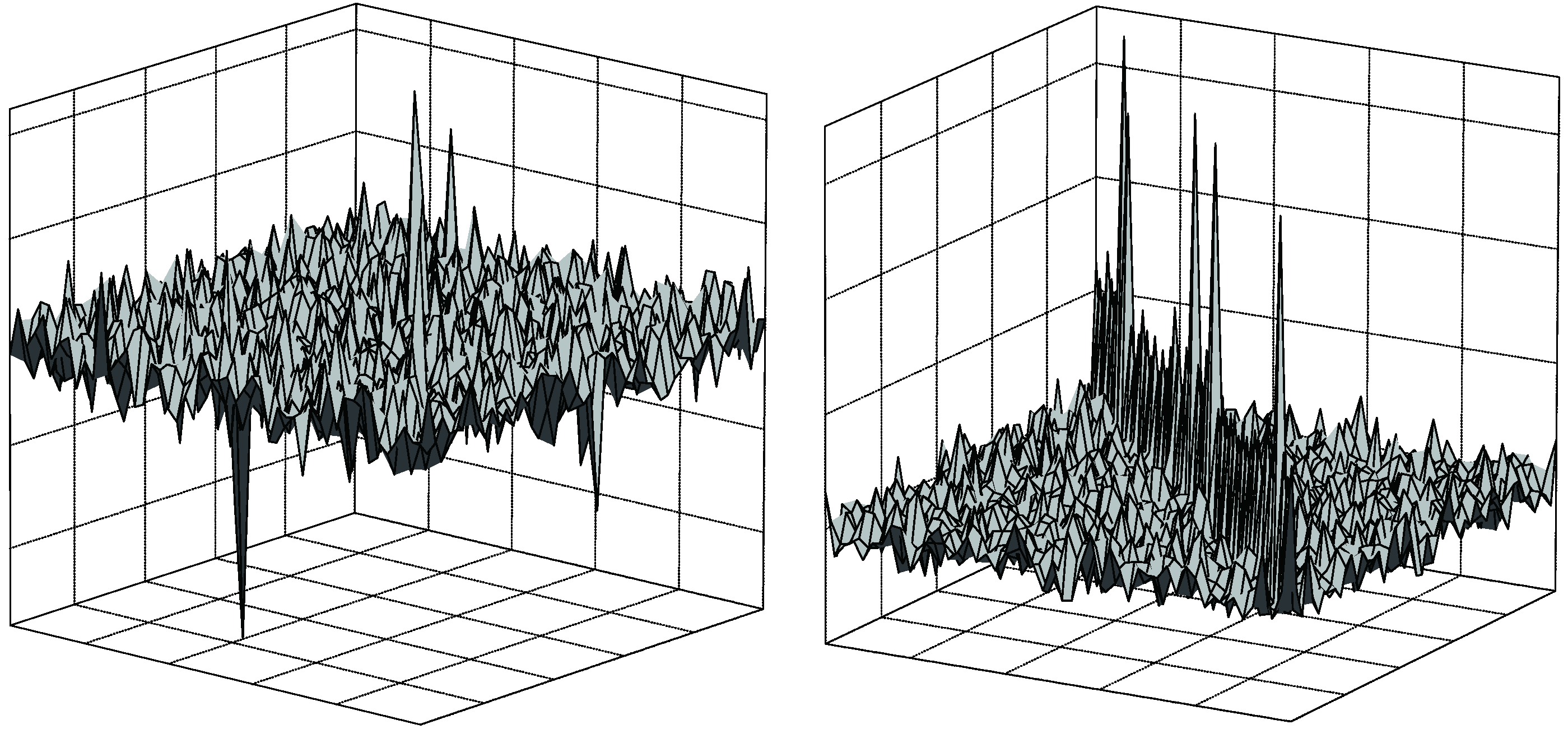
5.1. Influence on the Entries of the Covariance Matrix


| C-model and R-model | |||
|---|---|---|---|
| Matrices plots | ROC curves | ||
| Moderate IN | Strong IN | ||
| Signal-to-noise ratio (SNR) in dB | −10 | −10 | −10 |
| Number of primary transmitters (p) | 1 | 1 | 1 |
| Number of CRs (m) | 50 | 6 | 6 |
| Samples collected by each CR (n) | 50 | 50 | 50 |
| Impulsive to thermal noise power ratio (K) | 2 | 1 | 10 |
| Probability of impulsive noise (pIN) | 1 | 1 | 0.2 |
| Fraction of CRs hit by impulsive noise (pCR) | 0.1 | 0.5 | 0.5 |
| Samples affected by impulsive noise (Ns) | 3 | 10 | 10 |
| Number of impulsive noise bursts (Nb) | 1 | 1 | 1 |
| R-model | |||
| MA-filter length | L = 10 | ||
| AGC dynamic range | D = 2 | ||
| AGC overdrive fac | fod = 8 | ||
| Number of quantization levels | Nq = 8 | ||
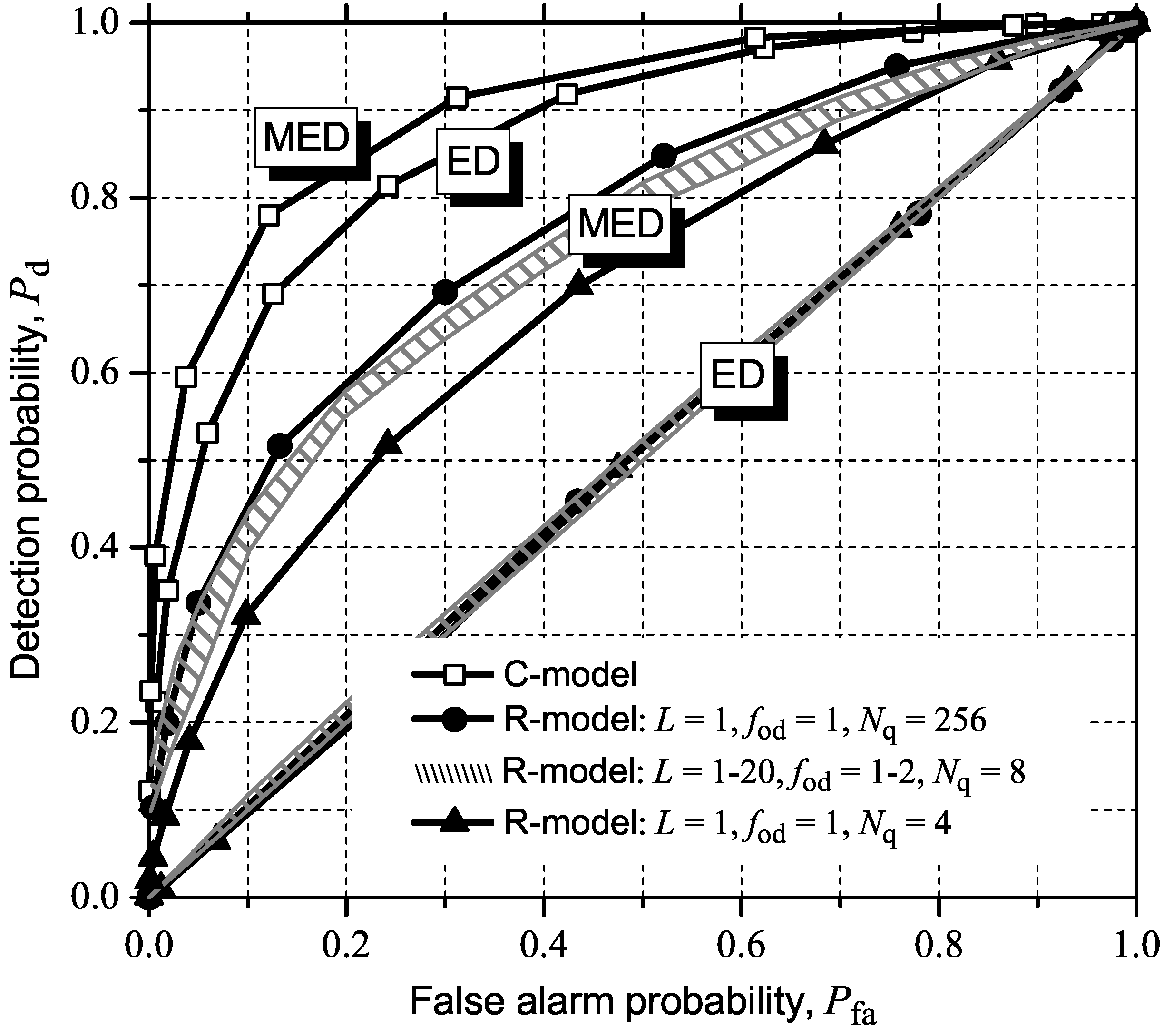
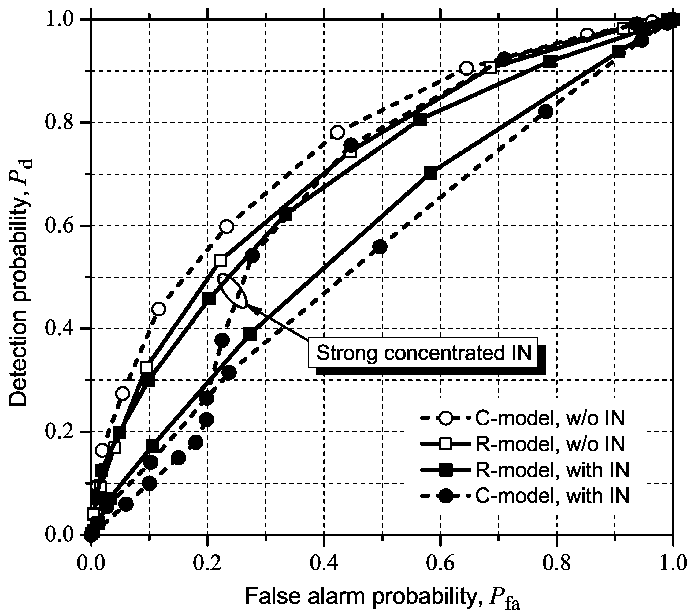
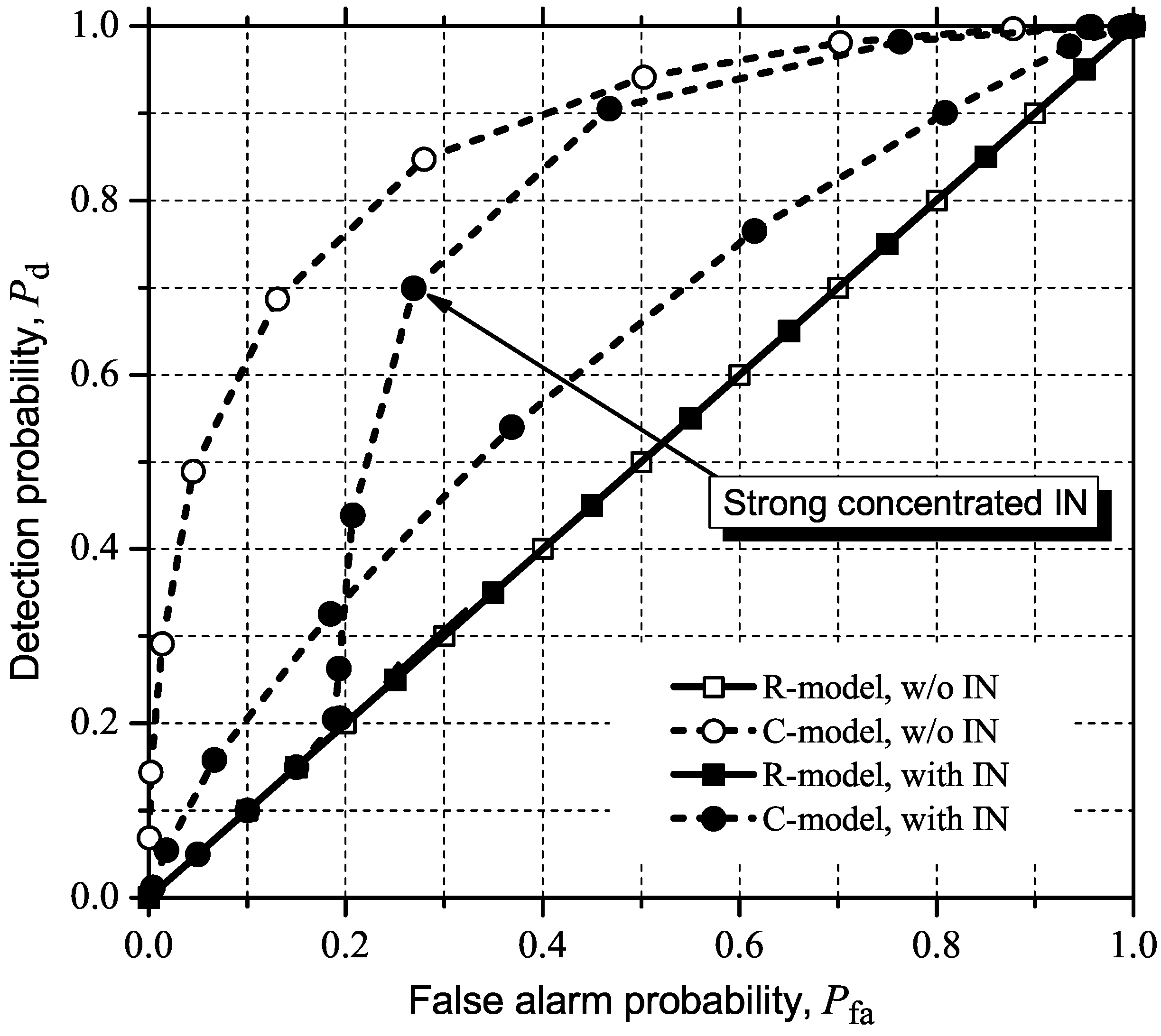
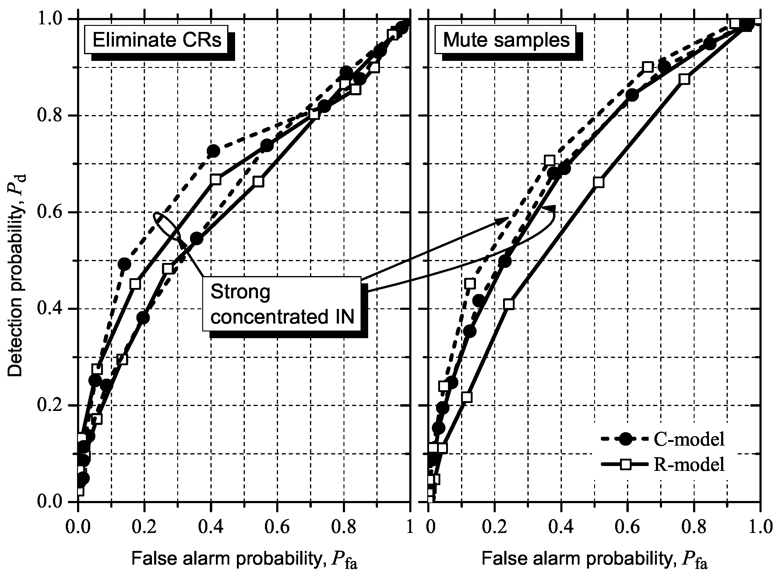
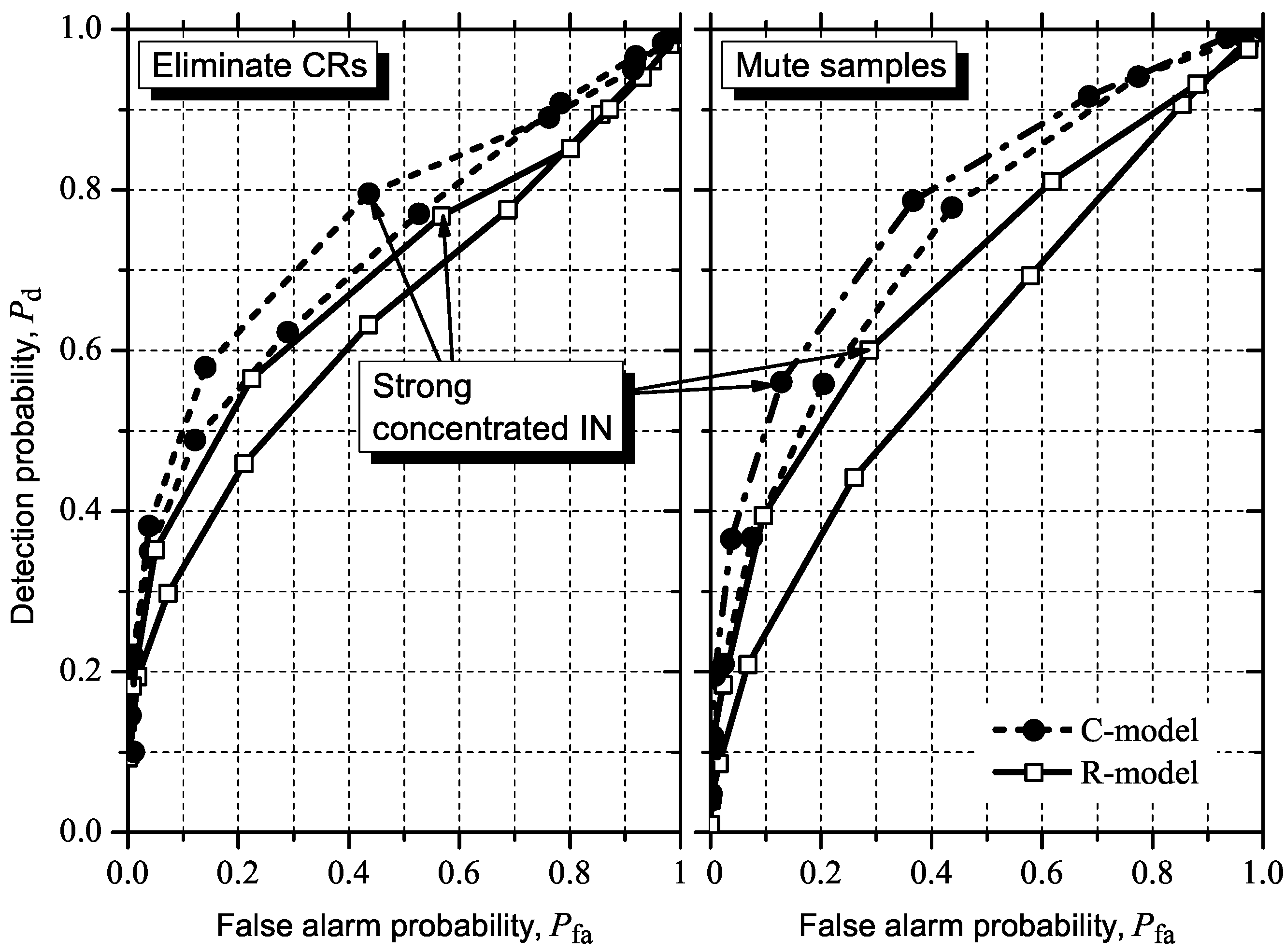
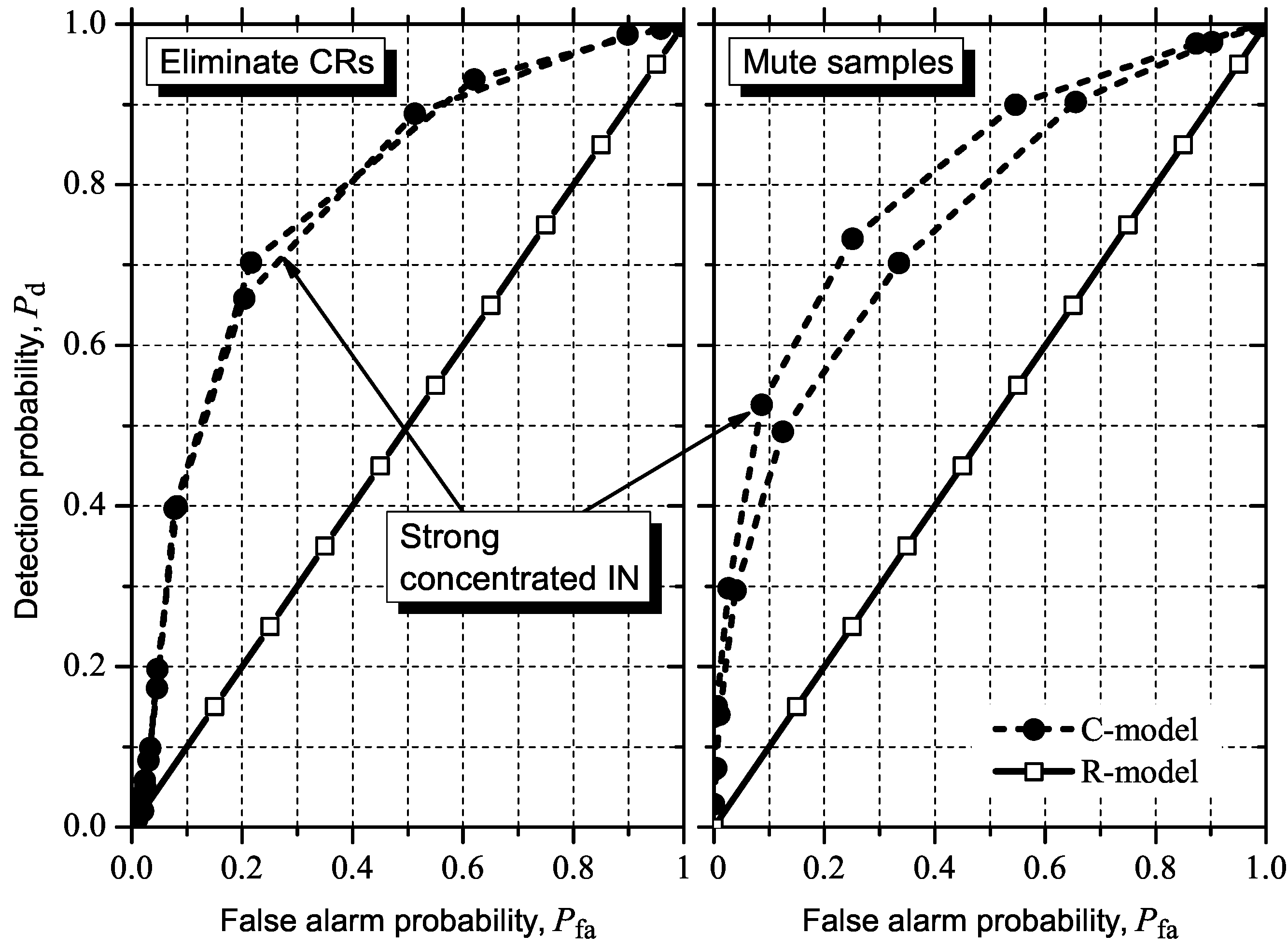
5.2. Influence of IN on ROC Curves
5.2.1. GLRT
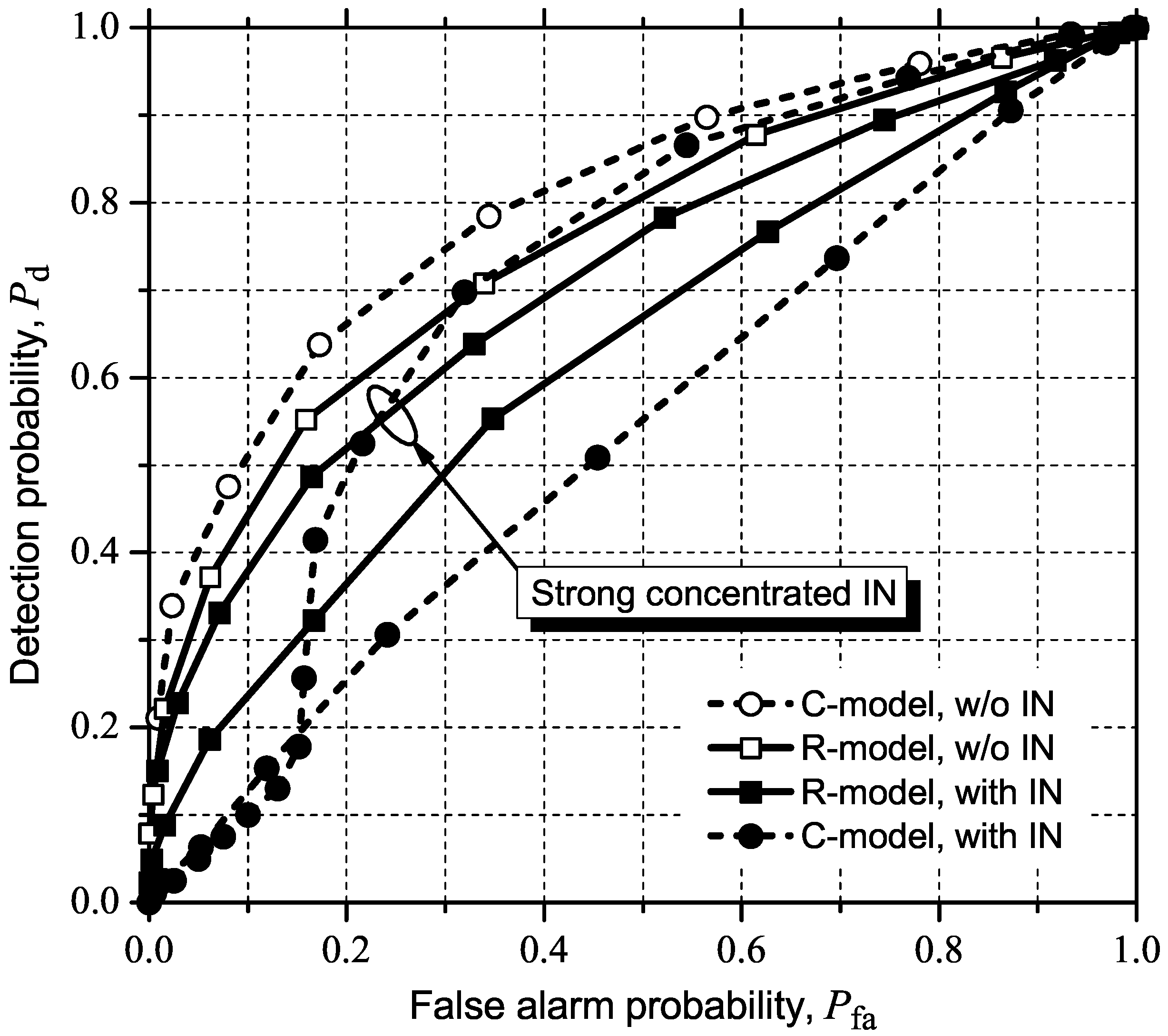
5.2.2. MMED (or ERD)
5.2.3. MED (or RLRT) and ED

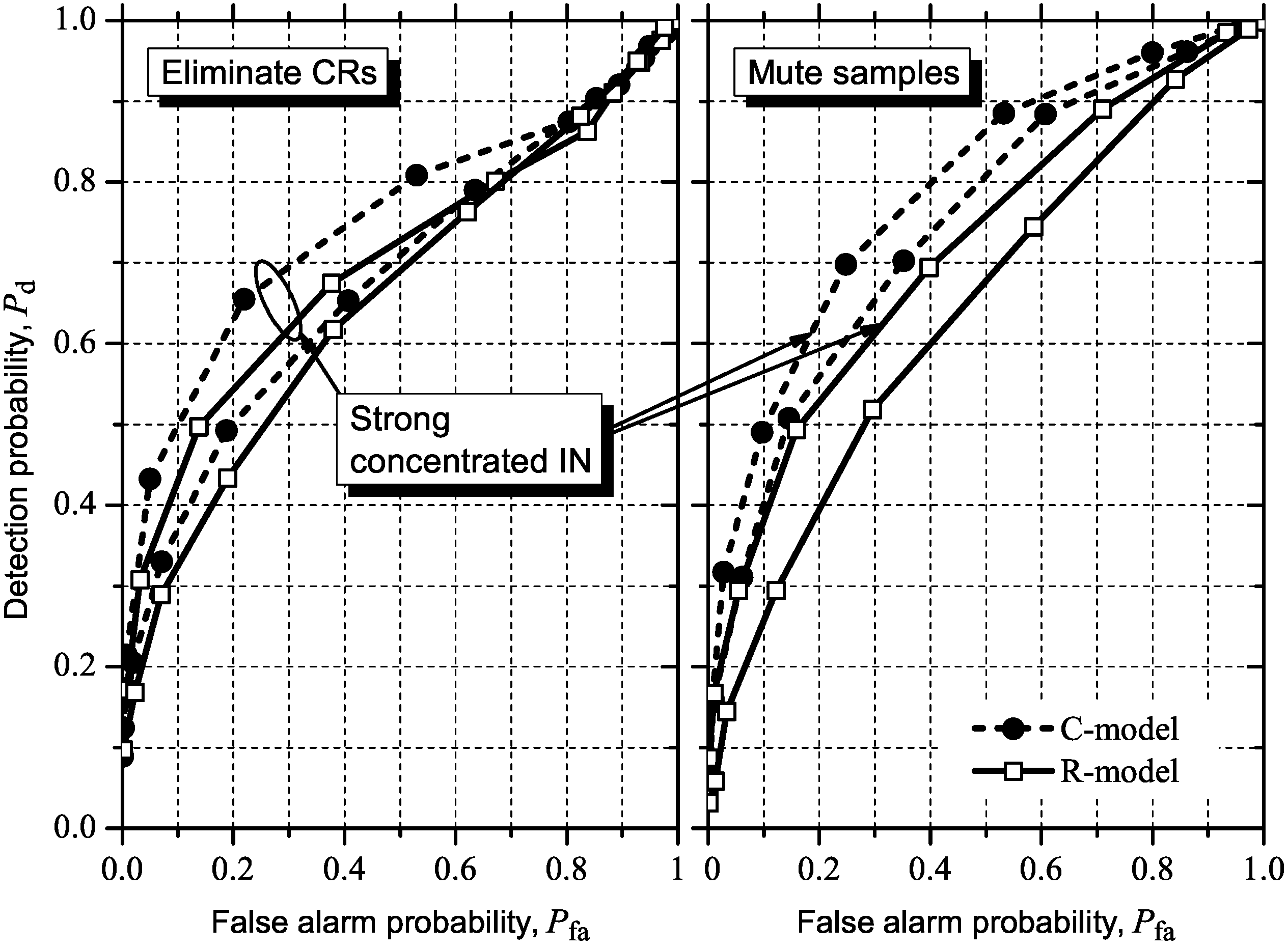
5.3. Detecting and Combating IN

6. Conclusions
Appendix

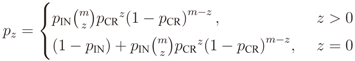
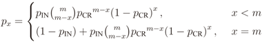
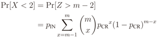
 is the binomial coefficient and where we have used the shorthand notations pz and px for Pr[Z = z] and Pr[X = x], respectively. Then we finally have

Supplementary Files
References
- Mitola, J., III.; Maguire, G., Jr. Cognitive radio: Making software radios more personal. IEEE Pers. Commun. 1999, 6, 13–18. [Google Scholar] [CrossRef]
- Qiu, R.; Guo, N.; Li, H.; Wu, Z.; Chakravarthy, V.; Song, Y.; Hu, Z.; Zhang, P.; Chen, Z. A unified multi-functional dynamic spectrum access framework: Tutorial, theory and multi-ghzwideband testbed. Sensors 2009, 9, 6835–6835. [Google Scholar] [CrossRef]
- Akyildiz, I.F.; Lo, B.; Balakrishnan, R. Cooperative spectrum sensing in cognitive radio networks: A survey. Phys. Commun. 2011, 4, 40–62. [Google Scholar] [CrossRef]
- Zeng, Y.; Liang, Y.-C. Eigenvalue-based spectrum sensing algorithms for cognitive radio. IEEE Trans. Commun. 2009, 57, 1784–1793. [Google Scholar] [CrossRef]
- Kortun, A.; Ratnarajah, T.; Sellathurai, M.; Zhong, C.; Papadias, C. On the performance of eigenvalue-based cooperative spectrum sensing for cognitive radio. IEEE J. Sel. Top. Signal Process. 2011, 5, 49–55. [Google Scholar] [CrossRef] [Green Version]
- Nadler, B.; Penna, F.; Garello, R. Performance of Eigenvalue-Based Signal Detectors with Known and Unknown Noise Level. In Proceedings of the 2011 IEEE International Conference on Communications, ICC, Kyoto, Japan, 5–9 June 2011; pp. 1–5.
- Liu, X. A survey on clustering routing protocols in wireless sensor networks. Sensors 2012, 12, 11113–11153. [Google Scholar] [CrossRef]
- Guimarães, D.A.; Souza, R.A.A. Implementation-oriented model for centralized data-fusion cooperative spectrum sensing. IEEE Commun. Lett. 2012, 16, 1804–1807. [Google Scholar] [CrossRef]
- Martinez-Rodriguez-Osorio, R.; de Haro-Ariet, L.; Calvo-Ramon, L.M.; Sanchez, M.G. Performance evaluation of W-CDMA in actual impulsive noise scenarios using adaptive antennas. IEEE Proc. Commun. 2004, 151, 589–594. [Google Scholar] [CrossRef]
- Budsabathon, M.; Hara, S. Robustness of OFDM Signal Against Temporally Localized Impulsive Noise. In Proceedings of the IEEE VTS 54th Vehicular Technology Conference, VTC 2001 Fall, Atlantic City, NJ, USA, 7–11 October 2001; Volume 3, pp. 1672–1676.
- Kang, H.G.; Song, I.; Yoon, S.; Kim, Y.H. A class of spectrum-sensing schemes for cognitive radio under impulsive noise circumstances: Structure and performance in nonfading and fading environments. IEEE Trans. Veh. Tech. 2010, 59, 4322–4339. [Google Scholar] [CrossRef]
- Pander, T. Application of weighted myriad filters to suppress impulsive noise in biomedical signals. TASK Quarterly 2004, 8, 199–216. [Google Scholar]
- Saarnisaari, H.; Henttu, P. Impulse Detection and Rejection Methods for Radio Systems. In Proceedings of the 2003 IEEE Military Communications Conference, MILCOM’03, Boston, MA, USA, 13–16 October 2003; Volume 2, pp. 1126–1131.
- Carrillo, R.; Aysal, T.; Barner, K. A Theoretical Framework for Problems Requiring Robust Behavior. In Proceedings of the 3rd IEEE International Workshop on Computational Advances in Multi-Sensor Adaptive Processing, CAMSAP, Aruba, Dutch Antilles, 13–16 December 2009; pp. 25–28.
- Sendora Project Public deliverable D4.1. Interference Model Based on Scenarios and System Requirements. Available online: http://www.sendora.eu/node/86 (accessed on 1 March 2012).
- Mashhour, A.; Domino, W.; Beamish, N. On the direct conversion receiver-a tutorial. Microw. J. 2001, 44, 114–128. [Google Scholar]
- Svitek, R.; Raman, S. DC offsets in direct-conversion receivers: Characterization and implications. IEEE Microw. Mag. 2005, 6, 76–86. [Google Scholar] [CrossRef]
- Razavi, B. Design considerations for direct-conversion receivers. IEEE Trans. Circuits Syst. II: Analog Digital Signal Process. 1997, 44, 428–435. [Google Scholar]
- Mailand, M.; Jentsche, H.J. Compensation of DC-Offsets and RF-Self-Mixing Products in Six-Port-Based Analog Direct Receivers. In Proceedings of the 14th IST Mobile & Wireless Comm. Summit, Dresden, Germany, 19–22 June 2005.
- Zheng, Y.; Tear, C.B.; Wong, S.J. DC Offset-Free RF Front-End Circuits and Systems for Direct Conversion Receivers. US Patent No. 7,164,901 B2, 2007. [Google Scholar]
- Mann, I.; McLaughlin, S.; Henkel, W.; Kirkby, R.; Kessler, T. Impulse generation with appropriate amplitude, length, inter-arrival, and spectral characteristics. IEEE J. Sel. Areas Commun. 2002, 20, 901–912. [Google Scholar] [CrossRef]
- Lago-Fernández, J.; Salter, J. Modeling Impulsive Interference in DVB-T: Statistical Analysis, Test Waveforms and Receiver Performance 2004. BBC R&D White Paper WHP 080.
- Middleton, D. Non-Gaussian noise models in signal processing for telecommunications: New methods an results for class A and class B noise models. IEEE Trans. Inf. Theory 1999, 45, 1129–1149. [Google Scholar] [CrossRef]
- Cichocki, A.; Amari, S. Adaptive Blind Signal and Image Processing; John Wiley and Sons, Inc.: Chichester, UK, 2002. [Google Scholar]
- IEEE Standard for Information Technology–Telecommunications and information exchange between systems Wireless Regional Area Networks (WRAN)–Specific requirements Part 22: Cognitive Wireless RAN Medium Access Control (MAC) and Physical Layer (PHY) Specifications: Policies and Procedures for Operation in the TV Bands. IEEE Std 802.22-2011, 2011, pp. 1–680
- Lim, T.J.; Zhang, R.; Liang, Y.C.; Zeng, Y. GLRT-Based Spectrum Sensing for Cognitive Radio. In Proceedings of the Global Telecommunications Conference, IEEE GLOBECOM 2008, New Orleans, LA, USA, 30 November–4 December 2008; pp. 1–5.
© 2013 by the authors; licensee MDPI, Basel, Switzerland. This article is an open-access article distributed under the terms and conditions of the Creative Commons Attribution license (http://creativecommons.org/licenses/by/3.0/).
Share and Cite
Guimarães, D.A.; De Souza, R.A.A.; Barreto, A.N. Performance of Cooperative Eigenvalue Spectrum Sensing with a Realistic Receiver Model under Impulsive Noise. J. Sens. Actuator Netw. 2013, 2, 46-69. https://doi.org/10.3390/jsan2010046
Guimarães DA, De Souza RAA, Barreto AN. Performance of Cooperative Eigenvalue Spectrum Sensing with a Realistic Receiver Model under Impulsive Noise. Journal of Sensor and Actuator Networks. 2013; 2(1):46-69. https://doi.org/10.3390/jsan2010046
Chicago/Turabian StyleGuimarães, Dayan A., Rausley A. A. De Souza, and André N. Barreto. 2013. "Performance of Cooperative Eigenvalue Spectrum Sensing with a Realistic Receiver Model under Impulsive Noise" Journal of Sensor and Actuator Networks 2, no. 1: 46-69. https://doi.org/10.3390/jsan2010046