Collaborative 3D Target Tracking in Distributed Smart Camera Networks for Wide-Area Surveillance

Abstract

With the evolution and fusion of wireless sensor network and embedded camera technologies, distributed smart camera networks have emerged as a new class of systems for wide-area surveillance applications. Wireless networks, however, introduce a number of constraints to the system that need to be considered, notably the communication bandwidth constraints. Existing approaches for target tracking using a camera network typically utilize target handover mechanisms between cameras, or combine results from 2D trackers in each camera into 3D target estimation. Such approaches suffer from scale selection, target rotation, and occlusion, drawbacks typically associated with 2D tracking. In this paper, we present an approach for tracking multiple targets directly in 3D space using a network of smart cameras. The approach employs multi-view histograms to characterize targets in 3D space using color and texture as the visual features. The visual features from each camera along with the target models are used in a probabilistic tracker to estimate the target state. We introduce four variations of our base tracker that incur different computational and communication costs on each node and result in different tracking accuracy. We demonstrate the effectiveness of our proposed trackers by comparing their performance to a 3D tracker that fuses the results of independent 2D trackers. We also present performance analysis of the base tracker along Quality-of-Service (QoS) and Quality-of-Information (QoI) metrics, and study QoS vs. QoI trade-offs between the proposed tracker variations. Finally, we demonstrate our tracker in a real-life scenario using a camera network deployed in a building.

1. Introduction

Smart cameras are evolving on three different evolutionary paths [1]. First, single smart cameras focus on integrating sensing with embedded on-camera processing power to perform various vision tasks on-board and deliver abstracted data from the observed scene. Second, distributed smart cameras (DSC) introduce distribution and collaboration of smart cameras resulting in a network of cameras with distributed sensing and processing. The main motivations for DSC are to (1) resolve occlusion; (2) mitigate the single camera handicap; and (3) extend sensing coverage. Finally, pervasive smart cameras (PSC) integrate adaptivity and autonomy to DSC.

Single camera tracking algorithms are often applied in the image plane. These image-plane (or 2D) trackers often run into problems such as target scale selection, target rotation, occlusion, view-dependence, and correspondence across views [2]. There are few 3D tracking approaches [2,3] that fuse results from independent 2D trackers to obtain 3D trajectories. These approaches employ decision-level fusion, where local decisions made by the node (i.e., 2D tracks) are fused to achieve global decision (i.e., 3D tracks), while discarding the local information (i.e., images captured at nodes). Because of the decision-level fusion, these approaches also suffer from all the problems associated with 2D tracking.

Tracking applications based on distributed and embedded sensor networks are emerging today, both in the fields of surveillance and industrial vision. The above-mentioned problems that are inherent in the image-plane based trackers can be circumvented by employing a tracker in 3D space using a network of smart cameras. Such smart camera networks can be employed using wireline or wireless networks. Wireless networks are more suited due to their easy deployment in complex environments. In wireless networks, traditional centralized approaches have several drawbacks, due to limited communication bandwidth and computational requirements, thus limiting the spatial camera resolution and the frame rate. The challenges for wireless smart camera networks include robust target tracking against scale variation, rotation and occlusion, especially in the presence of bandwidth constraints due to the wireless communication medium.

This paper presents an approach for collaborative target tracking in 3D space using a wireless network of smart cameras. The contributions of the paper are listed below:

• We define a target representation suitable for 3D tracking that includes the target state consisting of the position and orientation of the target in 3D space and the reference model consisting of multi-view feature histograms,
• We develop a probabilistic 3D tracker based on the target representation and implement the tracker based on sequential Monte Carlo methods,
• We develop and implement several variations of the base tracker that incur different computational and communication costs at each node, and produce different tracking accuracy. The variations include optimizations such as the use of mixture models, in-network aggregation and the use of image-plane based filtering where it is appropriate. We also present a qualitative comparison of the trackers according to their supported Quality-of-Service (QoS) and Quality-of-Information (QoI), and,
• We present quantitative evaluation of the trackers using synthetic targets in simulated camera networks, as well as using real targets (objects and people) in real-world camera network deployments. We also compare the proposed trackers with an implementation of a previous approach for 3D tracking, which is based on 3D ray intersection. The simulation results show robustness against target scale variation and rotation, while working within the bandwidth constraints.

The rest of the paper is organized as follows. In Section 2, we review some of the related work in the field. In Section 3, we briefly discuss some background for probabilistic target tracking. In Section 4, we detail the target representation and building blocks for the proposed tracking algorithm, which is presented in Section 4.2. In Section 5, we present a number of variations of the probabilistic tracker introduced in Section 4.2. Section 6 shows performance evaluation results, including a comparative evaluation of the proposed trackers in a simulated camera network, as well as real-life evaluation in two real-world camera network deployments tracking people and object moving in a building. We conclude in Section 7.

2. Related Work

Target tracking using a single or a network of smart cameras, also called visual surveillance, has become a very active research area in the field of computer vision and image processing in recent years. It is the key part of a number of applications such as automated surveillance, traffic monitoring, vehicle navigation, motion-based recognition, and human-computer interaction. In its simplest form, target tracking can be defined as the problem of estimating the trajectory and other desired properties, such as orientation, area, or shape of a target as it moves around in a scene. Most common challenges to target tracking are: (1) loss of information caused by projection of the 3D world on a 2D image; (2) noise in images; (3) complex target motion; (4) nonrigid or articulated nature of targets; (5) partial and full target occlusions; (6) complex target shapes; (7) scene illumination changes; and (8) real-time processing requirements of the tracking applications. In case of wireless and low-power, low-cost video sensors, additional challenges of resource-constrained devices include limited bandwidth, limited processing power, and limited battery-life.

A comprehensive survey on research in visual surveillance is conducted by Hu et al. [4]. The survey concludes with identifying future directions in visual surveillance, including occlusion handling, fusion of 2D and 3D tracking, 3D modeling of targets, and fusion of data from multiple video sensors. Another survey on target tracking using video sensors is presented in [5]. This work identifies three key aspects of any target tracking approach including target representation in terms of features, target detection based on the features, and a tracking algorithm that maintains and updates an estimate of target trajectory and other desired target properties.

2.1. Feature Selection for Tracking

The most desirable property of a visual feature, also called visual cue, is its uniqueness and discernibility, so that the objects can be easily distinguished in the feature space. Feature selection is closely related to object representation. For example, color is used as a feature for histogram-based appearance representations, while for contour-based representation, object edges are usually used as features. In general, many tracking algorithms use a combination of these features. The details of common visual features are as follows.

Motion In object tracking, motion feature refers to moving foreground in the video. The motion feature is computed by background subtraction via frame-differencing. Correct extraction of motion feature requires a robust and adaptive background model. There exist a number of challenges for the estimation of a robust background model [6], including gradual and sudden illumination changes, vacillating backgrounds, shadows, visual clutter, and occlusion. In practice, most of the simple motion detection algorithms have poor performance when faced with these challenges.

Color The apparent color of an object is influenced primarily by two physical factors: (1) the characteristics of the light source and (2) the surface reflectance properties of the object. In image processing, the RGB (red, green, blue) color space is usually used to represent color. However, the RGB space is not a perceptually uniform color space and is highly sensitive to illumination changes. HSV (hue, saturation, value) space, on the other hand, is approximately uniform in perception. The hue parameter in HSV space represents color information, which is illumination invariant as long as the following two conditions hold: (1) the light source color can be expected to be almost white; and (2) the saturation value of object color is sufficiently large [7].

The color feature is computed using one of two methods. In the simple model, the color of each pixel in the current image is compared with a prototype color $[h_0\left(t\right),s_0\left(t\right),v_0\left(t\right)]$ describing the color of the tracked object, e.g., face color in [8]. The pixels with acceptable deviation from the prototype color constitute the color cue. In a more complex model, the prototype color is modeled with adaptive mixture model. An adaptive Gaussian mixture model in hue-saturation space is used in [9].

Texture Visual textures are the patterns in the intensity variations of a surface. The patterns can be the result of physical surface properties such as roughness, or they could be the result of reflectance differences such as the color on a surface. Image texture is defined as a function of the spatial variation in pixel intensities. Texture is the most important visual feature in identifying different surface types, which is called texture classification. Image contrast, defined as the standard deviation of the grayscale values within a small image region, is considered a simple texture feature [9].

A number of other features such as shape-template [8], edge-maps [10], interest-points [11,12], and optical-flow [13] have been used for target representation.

2.2. Target Tracking

The aim of a target tracker is to maintain and update the trajectory of a target and other desired properties over time. The tasks of target detection and target association across time can either be performed separately or jointly. In the first case, possible targets in every frame are obtained using a target detection algorithm, and then the tracker associates the targets across frames. In the latter case, called joint data association and tracking, the targets and associations are jointly estimated by iteratively updating the target state. A tracking algorithm strongly depends on the target representation. Various target tracking approaches are described below.

Point Tracking When targets are represented as points, the association of the points is based on the previous target state that can include target position and motion. For single target tracking, Kalman filter and particle filters have been used extensively [14]. For multiple target tracking and data association, Kalman filter and particle filters are used in conjunction with a data association algorithm that associates the most likely measurement for a target to its state. Two widely used techniques for data association are Joint Probabilistic Data Association Filter (JPDAF) [15] and Multiple Hypothesis Tracking (MHT) [16].

Kernel Tracking Kernel refers to the target shape and appearance. Objects represented using shape and appearance models are tracked by computing the motion of the kernel in consecutive frames. This motion is usually in the form of a parametric transformation of the kernel, such as translation, rotation, and affine. Kernel tracking can also be called model-based tracking, since the kernel is actually target model. Kernel tracking approaches are based on templates and density-based appearance models used for target representation.

Templates and density-based appearance models have been widely used because of their relative simplicity and low computational cost. In kernel tracking, targets can be tracked individually or jointly. For single targets, the most common approach is template matching. Usually image intensity or color features are used to form the templates. Since image intensity is very sensitive to illumination changes, image gradients [17] can also be used as features. A limitation of template matching is its high computation cost due to the brute force search. Another approach called mean-shift tracker maximizes the appearance similarity iteratively by comparing the histograms of the target and the window around the hypothesized target location. Histogram similarity is defined in terms of the Bhattacharya coefficient [18,19].

In joint tracking of multiple targets, the interaction between targets is explicitly modeled, allowing the algorithm to handle partial or full occlusion of the targets. A target tracking method based on modeling the whole image as a set of layers is proposed in [20]. This representation includes a single background layer and one layer for each target. Each layer consists of shape priors (ellipse), motion model (translation and rotation), and layer appearance, (intensity modeled using a single Gaussian). Joint modeling of the background and foreground regions for tracking multiple targets is proposed in Bramble [21]. The appearance of background and all foreground targets are modeled by mixture of Gaussian. The shapes of targets are modeled as cylinders. It is assumed that the ground plane is known, thus the 3D target positions can be computed. Tracking is achieved by using particle filters where the state vector includes the 3D position, shape and the velocity of all targets in the scene.

A color-based probabilistic tracking approach is presented in [22]. The tracking algorithm uses global color reference models and endogenous initialization. This work implemented the tracker in a sequential Monte Carlo framework. Their approach defined a color likelihood function based on color histogram distances, the coupling of the color model with a dynamical state space model, and the sequential approximation of the resulting posterior distribution with a particle filter. The use of a sample-based filtering technique permits in particular the momentary tracking of multiple posterior modes. This is the key to escape from background distraction and to recover after partial or complete occlusions.

2.3. Tracking with Camera Networks

According to the overview paper [1], smart cameras are evolving on three different evolutionary paths. First, single smart cameras focus on integrating sensing with embedded on-camera processing power to perform various vision tasks on-board and deliver abstracted data from the observed scene. Second, distributed smart cameras (DSC) introduce distribution and collaboration resulting in a network of cameras with distributed sensing and processing. The main motivations for DSC are to (1) resolve occlusion; (2) mitigate single camera handicap; and (3) extend sensing coverage. Finally, pervasive smart cameras (PSC) integrate adaptivity and autonomy to DSC. According to the authors, the ultimate vision of PSC is to provide a service-oriented network that is easy to deploy and operate, adapts to changes in the environment and provides various customized services to users.

Single camera tracking algorithms are applied in the (2D) image-plane. These (2D) image-plane trackers often run into problems such as target scale selection, target rotation, occlusion, view-dependence, and correspondence across views [2]. There are few 3D tracking approaches [2,3] that fuse results from independent 2D trackers to obtain 3D trajectories. These approaches employ decision-level fusion, wherein local decisions made by the node (i.e., 2D tracks) are fused to achieve global decision (i.e, 3D tracks), while discarding the local information (i.e., images captured at nodes). Because of the decision-level fusion, these approaches also suffer from all the problems associated with 2D tracking.

Target Handoff An autonomous multicamera tracking approach based on a fully decentralized handover mechanism between adjacent cameras in presented in [23]. The system automatically initiates a single tracking instance for each target of interest. The instantiated tracker for each target follows the target over the camera network, migrating the target state to the camera that observed the target. This approach, however, utilizes data from a single camera node at any given time. The authors do admit that the effectiveness of their handover mechanism introduces some requirements for the tracker. First, the tracker must have short initialization time to build a target model. Second, the tracker on the new camera node must be able to initialize itself from a previously saved state, or handed-over state. Finally, the tracker must be robust with respect to the position and orientation of a target such that it must be able to identify the same target on the next camera node. These requirements need sophisticated and fine-tuned algorithms for 2D image-plane based tracking. A decentralized target tracking scheme built on top of a distributed localization protocol is presented in [24]. The protocol allows the smart camera nodes to automatically identify neighboring sensors with overlapping fields of view and facilitate target handoff in a seamless manner.

Another problem in 2D image-plane based trackers is the (re)initialization of a target when it (re)enters a camera field-of-view. In current state-of-the-art approaches, (re)initialization is performed by handing over target state to an adjacent camera node, which maintains the target state until it hands over the state to some other camera node. On the other hand, in 3D trackers, the target state and the target model are maintained in 3D space. The target state and the target model are not tied to the camera network parameters, such as the number of cameras, and position and orientation of the cameras. Once initialized, the target model does not need to be re-initialized as it moves in the sensing region and enters or re-enters a camera field-of-view.

3D Tracking Using Ray Intersection The classical approach for 3D collaborative target tracking is to combine the 2D tracking results from individual camera nodes for 3D tracking. This can be done by projecting rays from the camera center to the image affine coordinate in the world coordinate system and finding the intersection of multiple such rays from multiple cameras. This approach requires each camera node to maintain a 2D target model and a feature histogram. Hence the problems of scale variation, rotation and occlusion are not alleviated. As soon as the target moves along the camera principal axis, or rotates around its axis, the target model including the size and feature-histogram would become invalid. A target model learning algorithm during target tracking can help mitigate the problem but any sudden change that is faster than the model learning would cause the tracker to lose the target. An example of such approach is presented in [25].

Tracking Using 3D Models There are, however, a number of approaches that integrate 2D visual features with geometric constraints, such as ground plane, to build 3D likelihood of the targets. A tracker, called M2Tracker, for multi-camera system for tracking multiple people in a cluttered scene is presented in [26]. This work models the target using color models at different heights of the person being tracked, and probability of target being present in the horizontal plane at different heights. The position on horizontal plane is tracked using a Kalman filter. A distributed target tracking approach based on Kalman consensus filter for a dynamic camera network is presented in [27]. In this tracker, each camera comes to a consensus with its neighboring cameras about the actual state of the target.

An approach for 3D surveillance using a multi-camera system is presented in [28,29]. This paper proposes Probabilistic Occupancy Map (POM), which is a multi-camera generative detection method that estimates ground plane occupancy from multiple background subtraction views. Occupancy probabilities are iteratively estimated by fitting a synthetic model of the background subtraction to the binary foreground motion. This is similar to our work in terms of use of Bayesian estimation in a camera network system. However, there a number of differences between the two approaches. POM performs 2D occupancy estimation on a discretized grid-space, while our tracker estimates 3D position and orientation of a target in 3D space. The POM approach, as it is currently, assumes dynamic targets because of the use of background subtraction for target detection. On the other hand, we can track both static and dynamic targets. The POM approach integrates 2D visual features (i.e., moving foreground) with geometric constraints (i.e., ground plane estimate). Perhaps the biggest difference of all is that our algorithm is designed for resource-constrained wireless camera networks where the focus is minimal local-processing and communication of concise features to the base-station for heavier processing.

An approach for dynamic 3D scene understanding using a pair of cameras mounted on a moving vehicle is presented in [30]. Using structure-from-motion (SfM) self-localization, 2D target detections are converted to 3D observations, which are accumulated in a world coordinate frame. A subsequent tracking module analyzes the resulting 3D observations to find physically plausible space-time trajectories.

The Panoramic Appearance Map (PAM) presented in [31,32] is similar to our 3D target representation using multi-view histograms. PAM is a compact signature of panoramic appearance information of a target extracted from multiple cameras and accumulated over time. Both PAM and multi-view histograms are discrete representations, however PAM retains more spatial information than multi-view histograms. The use of additional spatial information can provide higher resolution in target orientation estimation.

3. Background

The two major components in a typical visual tracking system are the target representation and the tracking algorithm.

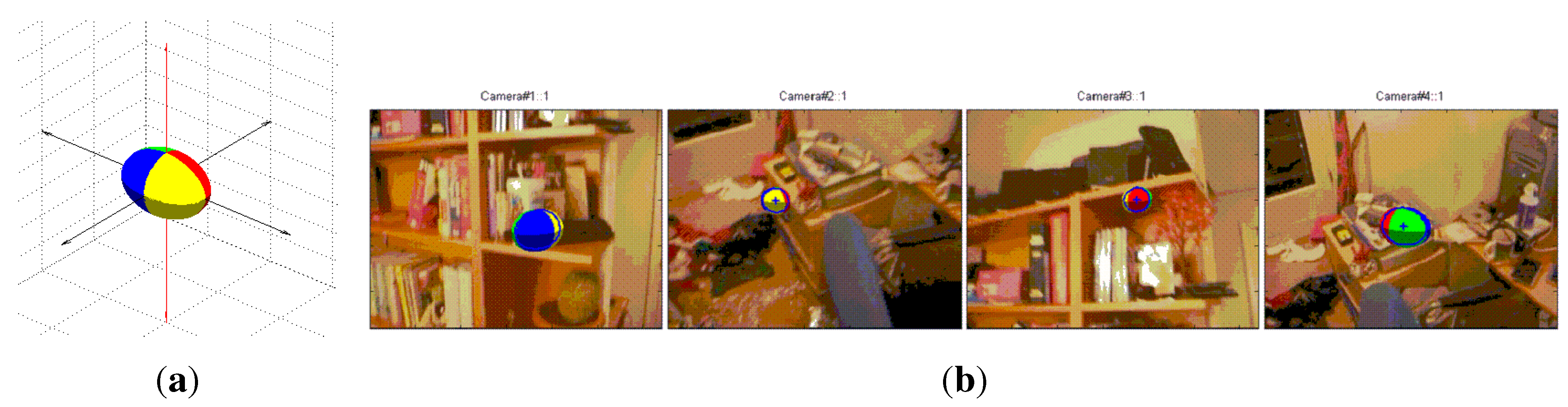
3.1. Target Representation

The target is represented by a reference model in the feature space. Typically, reference target models are obtained by histogramming techniques. For example, the model can be chosen to be the color, texture or edge-orientation histogram of the target. Red-Green-Blue (RGB) color space is taken as the feature space in [19], while Hue-Saturation-Value (HSV) color space is taken as the feature space in [22] to decouple chromatic information from shading effects.

3.1.1. Target Model

Consider a target region defined as the set of pixel locations ${\left\{{\mathbf{x}}_i\right\}}_{i=1\cdots p}$ in an image I. Without loss of generality, consider that the region is centered at $\mathbf{0}$. We define the function $b:{\mathbb{R}}^2\to \{1\cdots m\}$ that maps the pixel at location ${\mathbf{x}}_i$ to the index $b\left({\mathbf{x}}_i\right)$ of its bin in the quantized feature space. Within this region, the target model is defined as $\mathbf{q}={\left\{q_u\right\}}_{u=1\cdots m}$ with

$$\begin{array}{cc}\hfill q_u& =C\sum _{i=1}^{p}k(\parallel {\mathbf{x}}_i{\parallel }^2)\delta [b\left({\mathbf{x}}_i\right)-u]\hfill \end{array}$$

(1)

where δ is the Kronecker delta function, C is a normalization constant such that ${\sum }_{u=1}^m{q}_u=1$, and $k\left(x\right)$ is a weighting function. For example, in [19], this weighting function is an anisotropic kernel, with a convex and monotonic decreasing kernel profile that assigns smaller weights to the pixels farther from the center. If we set $w\equiv 1$, the target model is equivalent to the standard bin counting.

3.1.2. Target Candidate

A target candidate is defined similarly to the target model. Consider a target candidate at $\mathbf{y}$ as the region that is a set of pixel locations ${\left\{{\mathbf{x}}_i\right\}}_{i=1\cdots p}$ centered at $\mathbf{y}$ in the current frame. Using the same weighting function $k\left(x\right)$ and feature space mapping function $b\left(\mathbf{x}\right)$, the target candidate is defined as $\mathbf{p}\left(\mathbf{y}\right)={\left\{p_u\left(\mathbf{y}\right)\right\}}_{u=1\cdots m}$ with

$$\begin{array}{cc}\hfill p_u\left(\mathbf{y}\right)& =C\sum _{i=1}^{p}k(\parallel \mathbf{y}-{\mathbf{x}}_i{\parallel }^2)\delta [b\left({\mathbf{x}}_i\right)-u]\hfill \end{array}$$

(2)

where C is a constant such that ${\sum }_{u=1}^m{p}_u\left(\mathbf{y}\right)=1$.

3.1.3. Similarity Measure

A similarity measure between a target model $\mathbf{q}$ and a target candidate $\mathbf{p}\left(\mathbf{y}\right)$ plays the role of a data likelihood and its local maxima in the frame indicate the target state estimate. Since both the target model and the target candidate are discrete distributions, the standard similarity function is the Bhattacharya coefficient [18] defined as

$$\begin{array}{cc}\hfill \rho \left(\mathbf{y}\right)& \equiv \rho [\mathbf{p}\left(\mathbf{y}\right),\mathbf{q}]=\sum _{u=1}^m\sqrt{p_u\left(\mathbf{y}\right)q_u}\hfill \end{array}$$

(3)

We use the color model in HSV color space developed in [22]. HSV color space is approximately uniform in perception. The hue parameter in HSV space represents color information, which is illumination invariant as long as the following two conditions hold: (1) the light source color can be expected to be almost white; and (2) the saturation value of object color is sufficiently large [7]. We also use the texture model based on Local Binary Patterns (LBP) developed in [33]. The most important property of the LBP operator in real-world applications is its tolerance against illumination changes, and its computational simplicity, which makes it possible to analyze images in real-time settings.

4. Probabilistic 3D Tracker

In this section, we present the details of our proposed probabilistic 3D tracker. First, we describe the target representation including the target state and the target model. Then, we define the similarity measure for target localization. We then present an algorithm to estimate target orientation, and finally we present the details of the proposed tracker based on particle filtering.

4.1. Target Representation

A target is characterized by a state vector and a reference model. The target state consists of the position, velocity and orientation of the target in 3D space. The reference target model, described below, consists of the 3D shape attributes, and the multi-view histograms of the target object in a suitable feature-space. Such a reference target model would correspond to the actual 3D target, which does not change with scale variation and rotation. Once learned during the initialization phase, the model does not need to be updated or learned during tracking.

4.1.1. Target State

The state of a target is defined as

$$\begin{array}{c}\hfill \chi =[\mathbf{x},\mathbf{v},\mathit{\theta }]\end{array}$$

(4)

where $\mathbf{x}\in {\mathbb{R}}^3$ is the position, $\mathbf{v}\in {\mathbb{R}}^3$ is the velocity, and θ is the orientation of the target in 3D space. Specifically, we represent the target orientation as a unit quaternion, θ [34]. Target orientation can also be represented using Direction Cosine Matrix (DCM), rotation vectors, or Euler angles. Standard conversions between different representations are available. We chose unit quaternions due to their intuitiveness, algebraic simplicity, and robustness. The target state evolution (the target dynamics) is given by

$$\begin{array}{c}{\mathbf{x}}_t={\mathbf{x}}_{t-1}+{\mathbf{v}}_{t-1}·dt+w_{\mathbf{x}}\\ {\mathbf{v}}_t={\mathbf{v}}_{t-1}+w_{\mathbf{v}}\\ {\mathit{\theta }}_t\equiv {\mathit{\theta }}_{t-1}+w_{\mathit{\theta }}\end{array}$$

(5)

where $w_{\mathbf{x}}$, $w_{\mathbf{v}}$, and $w_{\mathit{\theta }}$ are the additive noise in target position, velocity and orientation, respectively.

4.1.2. Target Model

Since we want to model a 3D target, the definition of target model (see Equation (1)) as a single histogram on an image-plane is not sufficient. We extend the definition of the target model to include multiple histograms for a number of different viewpoints. This is called a multi-view histogram. Our target model is based on multi-view histograms in different feature spaces.

The 3D target is represented by an ellipsoid region in 3D space. Without loss of generality, consider that the target is centered at ${\mathbf{x}}_0={\left[000\right]}^{\mathrm{T}}$, and the target axes are aligned with the world coordinate frame. The size of the ellipsoid is represented by the matrix

$$\begin{array}{c}\hfill A=\left[\begin{array}{ccc}1/l^2& 0& 0\\ 0& 1/w^2& 0\\ 0& 0& 1/h^2\end{array}\right]\end{array}$$

(6)

where $l,w,h$ represent the length, width and height of the ellipsoid. A set $\mathcal{S}=\{{\mathbf{x}}_i:{\mathbf{x}}_i^{\mathrm{T}}A{\mathbf{x}}_i=1;{\mathbf{x}}_i\in {\mathbb{R}}^3\}$, is defined as the set of 3D points on the surface of the target. A function $b\left({\mathbf{x}}_i\right):\mathcal{S}\to \{1\cdots m\}$ maps the surface point at location ${\mathbf{x}}_i$ to the index $b\left({\mathbf{x}}_i\right)$ of its bin in the quantized feature space.

Let ${\left\{{\widehat{\mathbf{e}}}_j\right\}}_{j=1\cdots N}$ be the unit vectors pointing away from the target center. These unit vectors are the viewpoints from where the target is viewed and the reference target model is defined in terms of these viewpoints. Finally, the reference target model is defined as

$$\begin{array}{c}\hfill \mathbf{Q}=[{\mathbf{q}}_{{\widehat{\mathbf{e}}}_1}^{\mathrm{T}},{\mathbf{q}}_{{\widehat{\mathbf{e}}}_2}^{\mathrm{T}},\cdots {\mathbf{q}}_{{\widehat{\mathbf{e}}}_N}^{\mathrm{T}}]\end{array}$$

(7)

where ${\mathbf{q}}_{{\widehat{\mathbf{e}}}_j}$ is the feature-histogram for viewpoint ${\widehat{\mathbf{e}}}_j$, and N is the number of viewpoints. The feature histogram from viewpoint ${\widehat{\mathbf{e}}}_j$ is defined as ${\mathbf{q}}_{{\widehat{\mathbf{e}}}_j}={\{q_{{\widehat{\mathbf{e}}}_j,u}\}}_{u=1\cdots m}$

$$\begin{array}{c}\hfill q_{{\widehat{\mathbf{e}}}_j,u}=C\sum _{{\mathbf{x}}_i\in \mathcal{R}\left({\widehat{\mathbf{e}}}_j\right)}\kappa \left(d\left({\mathbf{y}}_i\right)\right)\delta [b\left({\mathbf{x}}_i\right)-u]\end{array}$$

(8)

where δ is the Kronecker delta function, C is the normalization constant such that ${\sum }_{u=1}^m{q}_{{\widehat{\mathbf{e}}}_j,u}=1$, $\kappa (·)$ is a weighting function, and

$$\begin{array}{cc}\hfill \mathcal{R}\left({\widehat{\mathbf{e}}}_j\right)& =\{{\mathbf{x}}_i:{\mathbf{x}}_i\in \mathcal{S},{\mathbf{x}}_i^{\mathrm{T}}A{\widehat{\mathbf{e}}}_j\ge 0,\forall i\ne j\to {\mathbf{y}}_i\ne {\mathbf{y}}_j\}\hfill \end{array}$$

(9)

is the set of points on the surface of the target that are visible from the viewpoint ${\widehat{\mathbf{e}}}_j$. In Equation (8), ${\mathbf{y}}_i=P_{{\widehat{\mathbf{e}}}_j}{\mathbf{x}}_i$ denotes the pixel location corresponding to the point ${\mathbf{x}}_i$ projected on the image plane, where $P_{{\widehat{\mathbf{e}}}_j}$ is the camera matrix for a hypothetical camera placed on vector ${\widehat{\mathbf{e}}}_j$ with principal axis along $-{\widehat{\mathbf{e}}}_j$. This camera matrix is defined as $P_{{\widehat{\mathbf{e}}}_j}=K\left[R|t\right]$, where $R,\mathbf{t}$ are the rotation and translation given as

$$\begin{array}{c}R=R_{\mathbf{x}}\left(\mathit{\theta }\right)R_{\mathbf{y}}\left(\varphi \right)R_0\\ \mathit{\theta }=si{n}^{-1}\left({\widehat{\mathbf{e}}}_{j,z}\right)\\ \varphi =ta{n}^{-1}\left(\frac{{\widehat{\mathbf{e}}}_{j,y}}{{\widehat{\mathbf{e}}}_{j,x}}\right)\\ R_0=\left[\begin{array}{ccc}0& 1& 0\\ 0& 0& -1\\ -1& 0& 0\end{array}\right]\end{array}$$

where $R_{\mathbf{x}}(.),R_{\mathbf{y}}(.)$ are the basic rotation matrices along $x-$ and $y-$axis, θ and ϕ are zenith and azimuth angles, respectively, and $R_0$ is the base rotation. The translation vector $\mathbf{t}$ is given as

$$\begin{array}{c}\mathbf{t}=-R{\mathbf{x}}_p\\ {\mathbf{x}}_p=L{\widehat{\mathbf{e}}}_j\end{array}$$

where ${\mathbf{x}}_p$ is the position of the hypothetical camera places on unit vector ${\widehat{\mathbf{e}}}_j$ at a distance L from the target. The function $d\left({\mathbf{y}}_i\right)$ in Equation (8) computes pixel distance between pixel locations ${\mathbf{y}}_i$ and ${\mathbf{y}}_0$ as

$$\begin{array}{c}\hfill d\left({\mathbf{y}}_i\right)={\left({\mathbf{y}}_i-{\mathbf{y}}_0\right)}^{\mathrm{T}}B\left({\mathbf{y}}_i-{\mathbf{y}}_0\right)\end{array}$$

(10)

where $B\in {\mathbb{R}}^{2\times 2}$ is the representation of size of the ellipse-like shape when the target ellipsoid is projected on the image plane, and ${\mathbf{y}}_0=P_{{\widehat{\mathbf{e}}}_j}{\mathbf{x}}_0$.

4.1.3. Similarity Measure and Localization

Below, we describe the algorithm to compute the similarity measure between the reference target model and a target candidate state using the camera images from a network of cameras.

Consider a camera network of N cameras, where the cameras are denoted as $C_n$. The camera matrices are denoted as $P_n=K\left[R_n|{\mathbf{t}}_n\right]$, where K is the internal calibration matrix, $R_n$ is the camera rotation and ${\mathbf{t}}_n$ is the camera translation. Consider an arbitrary target candidate state $\chi =[\mathbf{x},\mathbf{v},\mathit{\theta }]$, and let ${\left\{I_n\right\}}_{n=1\cdots N}$ be the images taken at the cameras at current time-step.

For the target candidate state χ, the similarity measure between the target candidate and the reference target model is computed based on the Bhattacharya coefficient. The similarity measure is defined as

$$\begin{array}{c}\hfill \rho \left(\chi \right)=\prod _{n=1}^N{\rho }_n\left(\chi \right)=\prod _{n=1}^N\rho \left({\mathbf{p}}_n\left(\mathbf{x}\right),{\mathbf{q}}_{{\widehat{\mathbf{e}}}_n}\right)\end{array}$$

(11)

where N is the number of cameras, ${\mathbf{p}}_n\left(\mathbf{x}\right)$ is the target candidate histogram at $\mathbf{x}$ from camera n, and ${\mathbf{q}}_{{\widehat{\mathbf{e}}}_n}$ is the target model for the viewpoint ${\widehat{\mathbf{e}}}_n$, where ${\widehat{\mathbf{e}}}_n$ is the viewpoint closest to camera $C_n$’s point-of-view. This is computed as

$$\begin{array}{c}\hfill {\widehat{\mathbf{e}}}_n=arg\underset{{\widehat{\mathbf{e}}}_j}{max}{\widehat{\mathbf{e}}}_{\mathrm{target}}^{\mathrm{T}}R\left(\mathit{\theta }\right){\widehat{\mathbf{e}}}_j\end{array}$$

(12)

where ${\widehat{\mathbf{e}}}_{\mathrm{target}}$ is the camera viewpoint towards the target, θ is the target orientation, and $R\left(\mathit{\theta }\right)$ is the rotation matrix for the target orientation given as

$$\begin{array}{cc}\hfill R\left(\mathit{\theta }\right)& =\left[\begin{array}{ccc}1-2{q_2}^2-2{q_3}^2& 2q_1{q}_2-2q_3{q}_4& 2q_1{q}_3+2q_2{q}_4\\ 2q_1{q}_2+2q_3{q}_4& 1-2{q_1}^2-2{q_3}^2& 2q_2{q}_3-2q_1{q}_4\\ 2q_1{q}_3-2q_2{q}_4& 2q_2{q}_3+2q_1{q}_4& 1-2{q_1}^2-2{q_2}^2\end{array}\right]\hfill \end{array}$$

(13)

where $\mathit{\theta }\equiv {\left[q_1,q_2,q_3,q_4\right]}^{\mathrm{T}}$ is the unit quaternion. The unit vector ${\widehat{\mathbf{e}}}_{\mathrm{target}}$ is given by

$$\begin{array}{c}\hfill {\widehat{\mathbf{e}}}_{\mathrm{target}}=\frac{{\mathbf{x}}_n-\mathbf{x}}{\parallel {\mathbf{x}}_n-\mathbf{x}\parallel }\end{array}$$

(14)

where ${\mathbf{x}}_n$ is the camera position.

The target candidate histogram ${\mathbf{p}}_n\left(\mathbf{x}\right)$ in Equation (11) is computed in a similar way as that for the target model histogram. The target candidate histogram for camera $C_n$ is given by

$$\begin{array}{c}\hfill {\mathbf{p}}_n\left(\mathbf{x}\right)={\left\{p_{n,u}\left(\mathbf{x}\right)\right\}}_{u=1\cdots m}\end{array}$$

(15)

where

$$\begin{array}{cc}\hfill p_{n,u}\left(\mathbf{x}\right)& =C\sum _{{\mathbf{y}}_i\in \mathcal{R}\left(\mathbf{x}\right)}\kappa \left(d({\mathbf{y}}_i,\mathbf{y})\right)\delta [b_I\left({\mathbf{y}}_i\right)-u]\hfill \end{array}$$

(16)

where C is the normalization constant such that ${\sum }_{u=1}^m{p}_{n,u}=1$, $\kappa (.)$ is the weighting function, and

$$\begin{array}{cc}\hfill \mathcal{R}\left(\mathbf{x}\right)& =\{{\mathbf{y}}_i:{\mathbf{y}}_i\in \mathcal{I},{({\mathbf{y}}_i-\mathbf{y})}^{\mathrm{T}}B\left(\mathbf{x}\right)({\mathbf{y}}_i-\mathbf{y})\le 1,\forall i\ne j\to {\mathbf{y}}_i\ne {\mathbf{y}}_j\}\hfill \end{array}$$

is the set of pixels in the region around $\mathbf{y}$, defined as $B\left(\mathbf{x}\right)$. Here, $\mathbf{y}=P_n\mathbf{x}$ is the projection of the target position on the camera image plane. The function $d({\mathbf{y}}_i,\mathbf{y})$ computes pixel distance between pixel locations ${\mathbf{y}}_i$ and $\mathbf{y}$ as follows,

$$\begin{array}{c}\hfill d({\mathbf{y}}_i,\mathbf{y})={\left({\mathbf{y}}_i-\mathbf{y}\right)}^{\mathrm{T}}B\left(\mathbf{x}\right)\left({\mathbf{y}}_i-\mathbf{y}\right)\end{array}$$

(17)

where $B\left(\mathbf{x}\right)\in {\mathbb{R}}^{2\times 2}$ is the representation of the size of the ellipse-like shape when the target ellipsoid is projected on the camera image plane.

4.1.4. Estimation of Target Orientation

Target orientation is estimated separately from the target position. Below, we describe our algorithm to estimate the target quaternion using the data from multiple cameras. In the first step, we estimate the target quaternion at each camera separately. In the second step, the individual target quaternions are fused together to get a global estimate of the target quaternion.

In the first step, on each camera, we compute the similarity measure of the target candidate histogram, ${\mathbf{p}}_n\left(\mathbf{x}\right)$, with each of the histograms in the target reference model (Equation (7))

$$\begin{array}{c}\rho \left(\chi \right)\equiv \left[{\rho }_1\left(\chi \right),{\rho }_2\left(\chi \right),\cdots {\rho }_N\left(\chi \right)\right]\\ {\rho }_j\left(\chi \right)\equiv \rho \left(\mathbf{p}\left(\mathbf{x}\right),{\mathbf{q}}_{{\widehat{\mathbf{e}}}_j}\right)\end{array}$$

where $\rho (\mathbf{p}\left(\mathbf{x}\right),{\mathbf{q}}_{{\widehat{\mathbf{e}}}_j})$ is the Bhattacharya coefficient. Now, we have viewpoints (${\widehat{\mathbf{e}}}_1,{\widehat{\mathbf{e}}}_2,\cdots ,{\widehat{\mathbf{e}}}_N$) and similarity measures (${\rho }_1,\cdots ,{\rho }_N$) along each viewpoint. We take the weighted average of all the viewpoints to get the most probable direction of the camera with respect to the target

$$\begin{array}{c}\hfill {\widehat{\mathbf{e}}}_{\mathrm{avg}}=\frac{{\sum }_j{\rho }_j{\widehat{\mathbf{e}}}_j}{{\sum }_j{\rho }_j}\end{array}$$

The unit vector $-{\widehat{\mathbf{e}}}_{\mathrm{avg}}$ is the estimate of the camera principal axis in the target’s frame of reference. To estimate the target rotation vector, we need to compute the transformation between $-{\widehat{\mathbf{e}}}_{avg}$ and ${\widehat{z}}_{\mathrm{CAM}}$, where ${\widehat{z}}_{\mathrm{CAM}}$ is the actual camera principal axis, and apply the same transformation to the target axes, $\mathbf{T}\equiv {\mathbf{I}}_{3\times 3}$, where ${\mathbf{I}}_{3\times 3}$ is the identity matrix of size 3.

The transformation between the two unit vectors can be computed as follows,

$$\begin{array}{c}\widehat{\mathbf{a}}=\frac{-{\widehat{\mathbf{e}}}_{avg}\times {\widehat{z}}_{\mathrm{CAM}}}{\parallel {\widehat{\mathbf{e}}}_{avg}\times {\widehat{z}}_{\mathrm{CAM}}\parallel }\\ \varphi ={\cos }^{-1}\left(-{\widehat{\mathbf{e}}}_{\mathrm{avg}}·{\widehat{\mathrm{z}}}_{\mathrm{CAM}}\right)\end{array}$$

where $\widehat{\mathbf{a}}$ is the Euler axis and ϕ is the rotation angle. Using this transformation, the transformed target axes are

$$\begin{array}{c}\hfill T\equiv R_{\widehat{\mathbf{a}}}\left(\varphi \right)=\left[{\widehat{\mathbf{e}}}_{x^{\prime }}^{\mathrm{T}}{\widehat{\mathbf{e}}}_{y^{\prime }}^{\mathrm{T}}{\widehat{\mathbf{e}}}_{z^{\prime }}^{\mathrm{T}}\right]\end{array}$$

(18)

The target orientation on each node is computed using the following conversion from Euler axis and rotation angle to quaternion

$$\begin{array}{cc}\hfill {\widehat{\mathit{\theta }}}_n& =\left[\begin{array}{c}{a}_{n,x}\sin ({\varphi }_{\mathrm{n}}/2)\\ a_{n,y}\sin ({\varphi }_{\mathrm{n}}/2)\\ a_{n,z}\sin ({\varphi }_{\mathrm{n}}/2)\\ \cos ({\varphi }_{\mathrm{n}}/2)\end{array}\right]\hfill \end{array}$$

(19)

In the second step, after we have estimated the target quaternions on each of the cameras, we fuse the quaternions together to get a global estimate of the target quaternion. Given target quaternion estimates ${\{{\widehat{\mathit{\theta }}}_n\}}_{n=1\cdots N}$ and weights ${\left\{w_n\right\}}_{n=1\cdots N}$ from N cameras, we estimate the global target quaternion by taking the weighted average

$$\begin{array}{cc}\hfill {\widehat{\mathit{\theta }}}_{all}& =\frac{{\sum }_n{w}_n{\widehat{\mathit{\theta }}}_n}{\parallel {\sum }_n{w}_n{\widehat{\mathit{\theta }}}_n\parallel }\hfill \end{array}$$

(20)

lease note that a single averaging of quaternion, such as in Equation (20), may be sufficient if the individual quaternions are clustered together. A quaternion-outlier detection method can be applied to ensure that quaternions being averaged are indeed clustered together. However, we do recognize that an averaging method such as presented in [35] can be utilized to estimate average quaternion, particularly when the individual quaternions from camera nodes are not clustered together. The current target orientation is updated using the global target orientation estimated from the camera images as

$$\begin{array}{c}\hfill \widehat{\mathit{\theta }}=\alpha {\widehat{\mathit{\theta }}}_{all}+(1-\alpha ){\widehat{\mathit{\theta }}}_{prior}\end{array}$$

where ${\widehat{\mathit{\theta }}}_{prior}$ is the prior target orientation and α is an update factor.

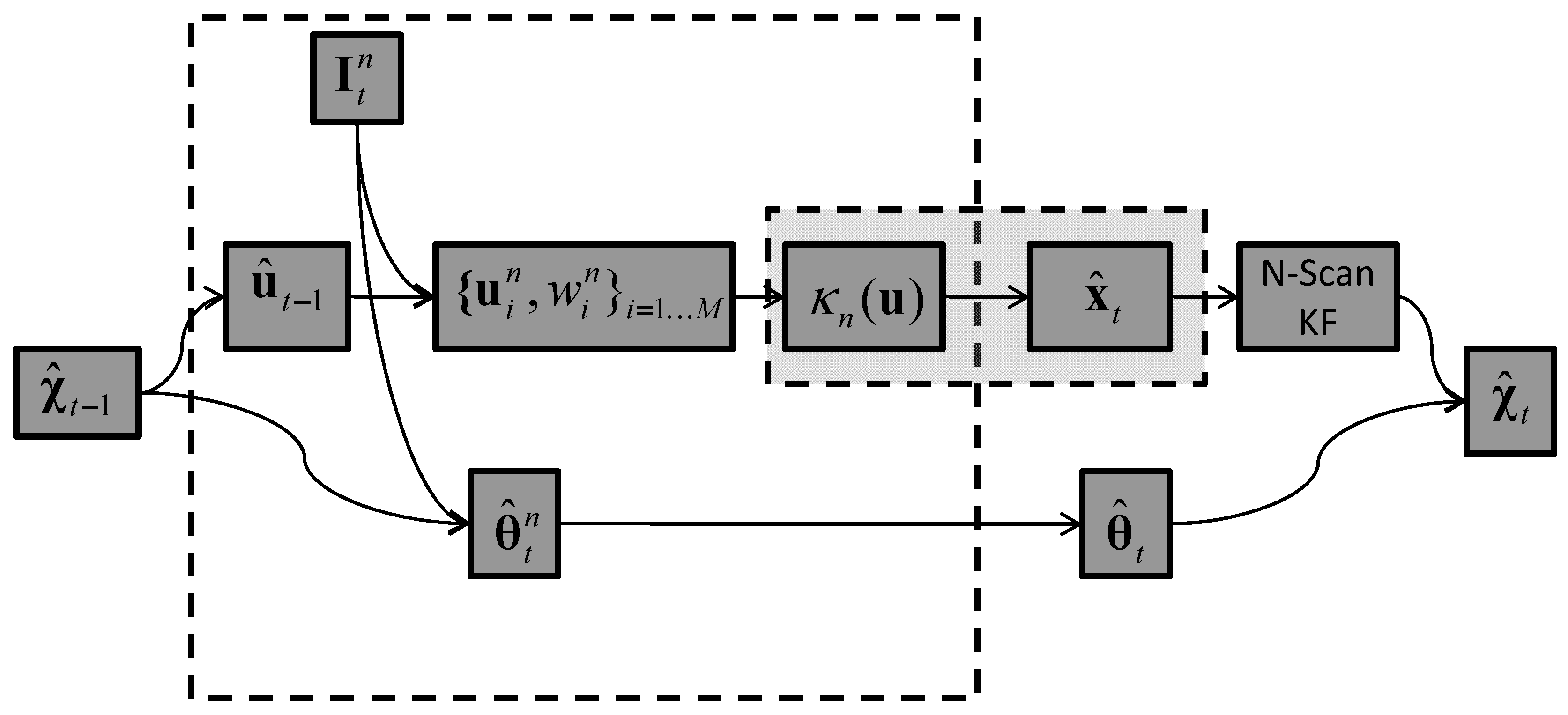
4.2. Tracking Algorithm

In this section, we discuss the implementation of our base tracker.

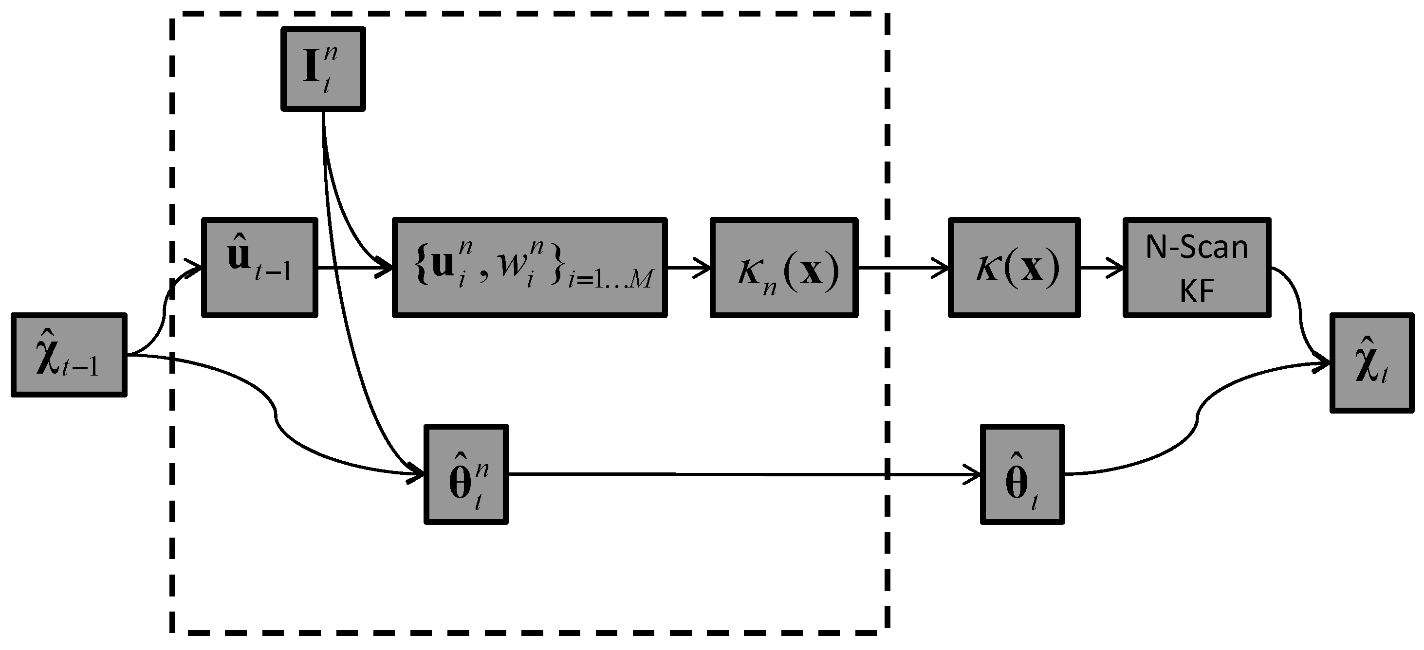
4.2.1. Base Tracker (T0)

Our probabilistic 3D tracker is based on sequential Bayesian estimation. In Bayesian estimation, the target state is estimated by computing the posterior probability density $p\left(x_{t+1}\right|z_{0:t+1})$ using a Bayesian filter described by

$$\begin{array}{c}\hfill p\left(x_{t+1}\right|z_{0:t+1})\propto p\left(z_{t+1}\right|x_{t+1}){\int }_{x_t}p\left(x_{t+1}\right|x_t)p\left(x_t\right|z_{0:t})d{x}_t\end{array}$$

(21)

where $p\left(x_t\right|z_{0:t})$ is the prior density, $p\left(z_{t+1}\right|x_{t+1})$ is the likelihood given the target state, and $p\left(x_{t+1}\right|x_t)$ is the prediction for the target state $x_{t+1}$ given the current state $x_t$ according to a target state evolution model. Here $z_{0:t}\equiv {(z_0,\cdots ,z_t)}^{\mathrm{T}}$ denote all the measurements up until t.

In sequential Bayesian estimation, the target state estimate can be updated as the data is made available using only the target state estimate from the previous step, unlike Bayesian estimation, where the target state estimate is updated using all the data collected up until the current time-step. In sequential Bayesian estimation, the target state is estimated by computing the posterior probability density $p\left(x_{t+1}\right|z_{t+1},x_t)$ using a sequential Bayesian filter described by

$$\begin{array}{c}\hfill p\left(x_{t+1}\right|z_{t+1},x_t)\propto p\left(z_{t+1}\right|x_{t+1})p\left(x_{t+1}\right|x_t)p\left(x_t\right)\end{array}$$

(22)

where $p\left(x_t\right)$ is the prior density from the previous step, $p\left(z_{t+1}\right|x_{t+1})$ is the likelihood given the target state, and $p\left(x_{t+1}\right|xt)$ is the prediction for the target state $x_{t+1}$ given the current state $x_t$ according to a target state evolution model.

In visual tracking problems the likelihood is non-linear and often multi-modal. As a result linear filters such as the Kalman filter and its approximations are usually not suitable. Our base tracker is implemented using particle filters. Particle filters can handle multiple hypotheses and non-linear systems. Our probabilistic base tracker is summarized in Algorithm 1. Figure 1 illustrates the base tracker operation for a single time-step. At each time step, each camera node performs position estimation and orientation estimation separately. For position estimation, we generate a set of synchronized particles for the predicted position. The synchronized particle set is generated using a synchronized random number generator, which can be achieved by seeding the random number generator on each node with the same seed. Then, target candidate histograms are computed for each of the proposed particles. In our framework, we use color features, specifically HS color space, and texture features, specifically LBP. After we compute the target candidate histograms in HS-space and LBP-space for each particle, we compute the weights according to the following

$$\begin{array}{c}\hfill \rho \left(\mathbf{x}\right)={\alpha }_{\mathrm{HS}}{\rho }_{\mathrm{HS}}\left(\mathbf{x}\right)+(1-{\alpha }_{\mathrm{HS}}){\rho }_{\mathrm{LBP}}\left(\mathbf{x}\right)\end{array}$$

(23)

where ${\rho }_{\mathrm{HS}}\left(\mathbf{x}\right)$ and ${\rho }_{\mathrm{LBP}}\left(\mathbf{x}\right)$ are the similarity measures for the target candidate histograms in HS- and LBP-spaces, respectively (computed using Equation (11)), and $0\le {\alpha }_{\mathrm{HS}}\le 1$ is the weighting factor. Target orientation estimation is performed on each camera node according to the algorithm described earlier in the section.

Algorithm 1 Base tracker

1: Input: The reference target model $\mathbf{Q}$ (Equation (7)), and target state ${\widehat{\chi }}_0=[{\widehat{\mathbf{x}}}_0,{\widehat{\mathbf{v}}}_0,{\widehat{\mathit{\theta }}}_0]$ from previous time-step. 2: /*** On Each Camera Node: ${\left\{C_n\right\}}_{n=1\cdots N}$ ***/ 3: /* Target Position Estimation */ 4: Generate synchronized particle set for the target position, ${\left\{{\tilde{\mathbf{x}}}_i\right\}}_{i=1\cdots M}\sim \mathcal{N}({\widehat{\mathbf{x}}}_0+{\widehat{\mathbf{v}}}_0,\Sigma )$, 5: For $i=1\cdots M$, 6:      Compute target candidate histogram, ${\mathbf{p}}_n\left({\tilde{\mathbf{x}}}_i\right)$ according to Equation (15), 7:      Compute weights $w_{n,i}={\rho }_n\left({\tilde{\mathbf{x}}}_i\right)$ according to Equation (11), 8:      Communicate weights $w_{n,i}$ to the Base-Station 9: /* Target Orientation Estimation */ 10: Estimate target orientation ${\widehat{\mathit{\theta }}}_n$ according to Equation (19) 11: /*** On Base Station: ***/ 12: For $i=1\cdots M$, combine weights from each camera, $w_i={\prod }_n{w}_{n,i}$, 13: Compute target position estimate, $\widehat{\mathbf{x}}$ 14: Compute target velocity estimate, $\widehat{\mathbf{v}}$ using Kalman filter, 15: Estimate target orientation θ according to Equation (21).

Figure 1. Proposed base tracker T0 for video tracking.

Figure 1. Proposed base tracker T0 for video tracking.

Then, the weights of the synchronized particle set from each of the camera nodes are sent to the base-station, and are combined together. An MMSE, MLE or MAP estimate is estimated as

$$\begin{array}{c}\mathrm{MMSE}:\widehat{\mathbf{x}}=\frac{{\sum }_i{w}_i{\mathbf{x}}_i}{{\sum }_i{w}_i}\end{array}$$

(24)

$$\begin{array}{c}\mathrm{MLE}:\widehat{\mathbf{x}}=\arg \underset{\mathbf{x}}{\max }{w}_i\end{array}$$

(25)

$$\begin{array}{c}\mathrm{MAP}:\widehat{\mathbf{x}}=\arg \underset{\mathbf{x}}{\max }{w}_i\mathcal{N}\left({\mathbf{x}}_i\right|{\mathbf{x}}_0,{\Sigma }_0)\end{array}$$

(26)

The target position estimate is then used in an N-scan Kalman smoother [36] to smooth the position estimates, as well as to estimate the target velocity. Finally, target orientation estimates from each camera node are combined according to Equation (21) to estimate global target orientation.

Computational Cost Each camera node generates a synchronized particle set of size M and computes weights for each particle. Computation of weight for a single particle includes computing the target candidate histogram and the Bhattacharya coefficient with the reference target model. Hence, the total computational cost at each time-step on each camera node is $O\left(Mm{n}_p\right)$, where M is the number of particles, m is the number of bins in the quantized feature-space, and $n_p$ is the number of pixels inside the target candidate region.

Communication Cost The base tracker algorithm requires the base station to transmit the current target state to each camera node. Each camera node then transmits the weights for the synchronized particle set back to the base station, as well as the target orientation estimates. During a single time-step, the total cost of communication can be computed as follows. Let the size of the target state $\chi =\{\mathbf{x},\mathbf{v},\mathit{\theta }\}$ be $24+24+32=80$ bytes, and each particle weight be represented by an 8 byte double. Then, the total cost of communication during a single step is $C=\left|\chi \right|+MN\left|w\right|=80+8MN$ bytes, where N is the number of cameras and M is the number of particles in the synchronized particle filter. For example, if $N=4$ and $M=1000$, then the total cost is $C=32,080$ bytes, or approximately 32 kb-per-time-step. If the application is running at 4 Hz, then the total bandwidth consumption would be around 128 kbps.

5. Tracker Variations

In this section, we introduce four variations to the base tracker introduced in Section 4.2. These variations incur different computational and communication costs on each node, and produce different tracking accuracies. The computational and communication costs associated with a tracker directly affects the tracking rate, network size, bandwidth consumption, latency, etc. In other words, different trackers support different Quality-of-Service (QoS). Since the objective of a tracking algorithm is to effectively track a target, which is the information that is desired from a tracking algorithm, we can say that different trackers support different Quality-of-Information (QoI). After the description of all the tracker variations, we qualitatively classify the trackers according to their supported QoS and QoI.

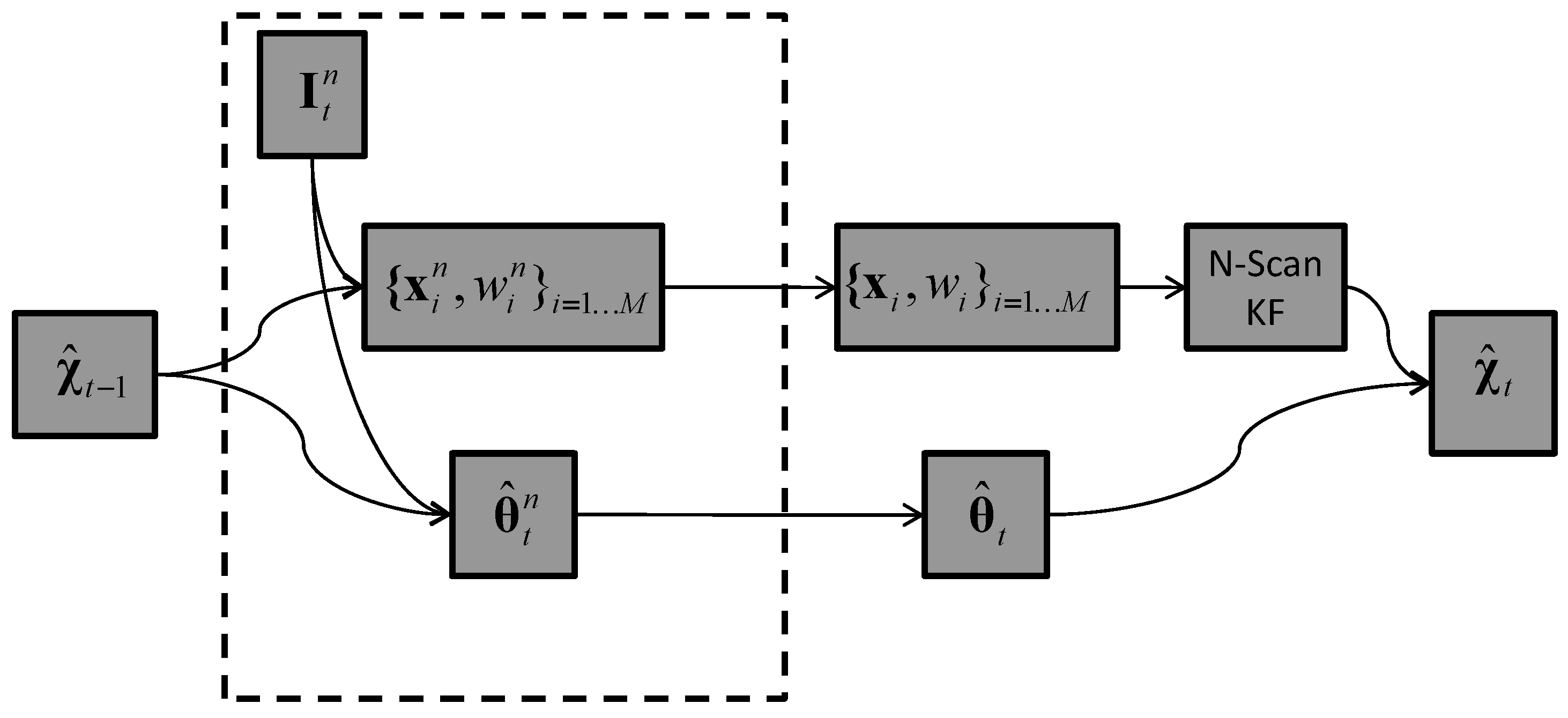
5.1. Tracker T1: 3D Kernel Density Estimate

In the base tracker, the communication cost is very high because we send weights for the synchronized particle set from each node to the base station. In this variation of the base tracker, instead of sending all the weights, each node computes a 3D kernel density estimate, approximates the kernel density estimate using a Gaussian Mixture Model (GMM), and sends only the mixture model parameters to the base station, thereby reducing the communication cost by a large factor. Figure 2 shows the tracker. In tracker T1, the main differences from tracker T0 are: (1) computation of the 3D kernel density from the particle set; (2) GMM approximation of the kernel density; and (3) state estimation at the base station using GMM parameters from all nodes.

The kernel density in 3D space is computed as follows

$$\begin{array}{cc}\hfill \kappa \left(\mathbf{x}\right)& =\sum _{i=1}^{N}k\left(\frac{\parallel \mathbf{x}-{\mathbf{x}}_i{\parallel }^2}{h^2}\right)\hfill \end{array}$$

(27)

where $k\left(x\right)=\exp \left(-x/2\right):[0,\infty )\to \mathbb{R}$ is the kernel profile function. The 3D kernel density $\kappa \left(\mathbf{x}\right)$ is approximated as a 3D-GMM of appropriate model-order (number of mixture components). A model-order selection algorithm is used to select an optimal model-order that best matches the kernel density. The best matching is done according to Kullback–Leibler (KL) divergence as follows

$$\begin{array}{cc}\hfill m_{opt}& =arg\underset{m\le m_{\mathrm{MAX}}}{min}\mathrm{KL}\left(\kappa \left(\mathbf{x}\right)\left|\right|g_m\left(\mathbf{x}\right)\right)\hfill \end{array}$$

(28)

where $g_m\left(\mathbf{x}\right)\equiv {\{{\alpha }_i,{\mu }_i,{\Sigma }_i\}}_{i=1\cdots m}$ is the 3D-GMM of order m (estimated using the EM algorithm [37]), $\mathrm{KL}\left(\kappa \left(\mathbf{x}\right)\right|\left|g_m\left(\mathbf{x}\right)\right)$ is the KL-divergence of $g_m\left(\mathbf{x}\right)$ from $\kappa \left(\mathbf{x}\right)$, and $m_{opt}$ is the optimal model-order.

Figure 2. Tracker T1. The tracker uses 3D kernel density estimate.

Figure 2. Tracker T1. The tracker uses 3D kernel density estimate.

Please note that a large value for parameter $m_{\mathrm{MAX}}$ would be able to capture a complex distribution more accurately, but at the cost of computational complexity as well as higher communication cost. However, for simpler distributions, the optimal value for $m=m_{opt}$ may not be the largest possible value $m_{\mathrm{MAX}}$. Finally, the state estimation is done at the base station by mode estimation on the combined kernel density from all the nodes

$$\begin{array}{cc}\hfill \widehat{\mathbf{x}}& =arg\underset{\mathbf{x}}{max}\kappa \left(\mathbf{x}\right)\equiv arg\underset{\mathbf{x}}{max}\sum _{i=1}^{m_{opt}}{\alpha }_i\mathcal{N}\left(\mathbf{x}\right|{\mu }_i,{\Sigma }_i)\hfill \end{array}$$

(29)

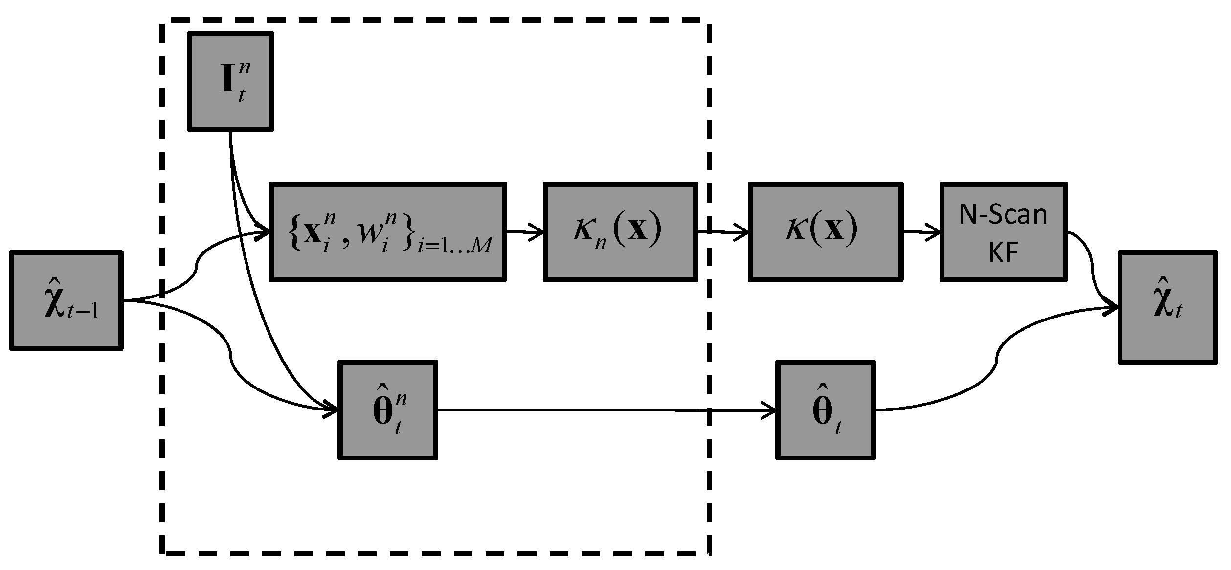
5.2. Tracker T2: In-Network Aggregation

Further improvements in terms of the communication cost can be made by in-network aggregation. In this tracker, instead of each camera node sending the mixture model parameters to the base station, in-nodes in the routing tree aggregate the mixture model parameters and forward a fewer number of parameters.

Figure 3 shows the tracker. In-network aggregation is done in two-steps. In the first step, the GMMs from multiple camera nodes are combined by taking the product of the GMMs. In the second step, we reduce the number of mixture components in the resulting GMM from the first step to fit the size of a message of fixed size.

Figure 3. Tracker T2 design. (a) Tracker T1 does not include in-network aggregation; whereas (b) tracker T2 includes in-network aggregation.

Figure 3. Tracker T2 design. (a) Tracker T1 does not include in-network aggregation; whereas (b) tracker T2 includes in-network aggregation.

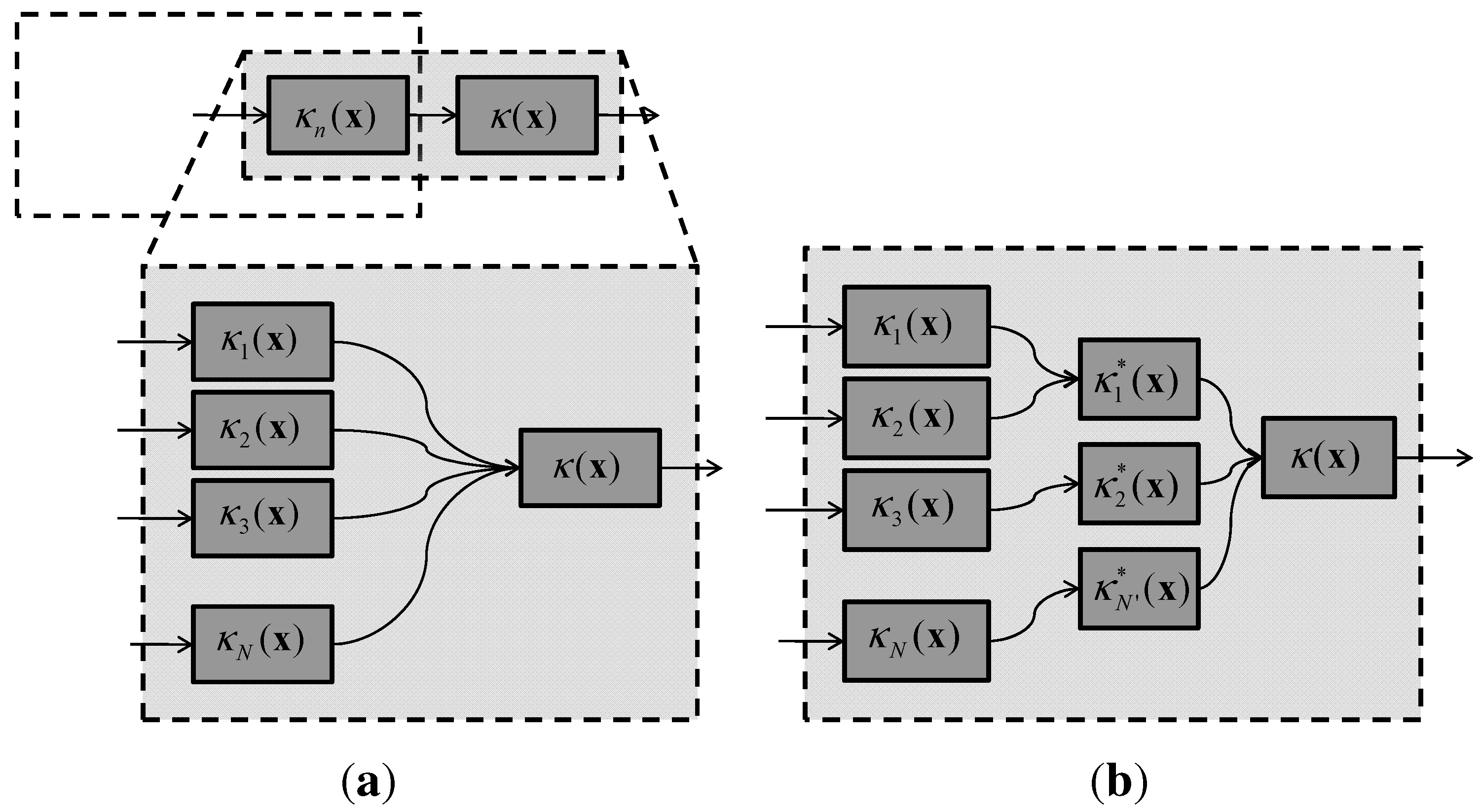
5.2.1. Step 1: Product of GMMs

Let ${\left\{{\kappa }_j\left(\mathbf{x}\right)\right\}}_{j=1\cdots N}$ be the kernel densities available at a node from its children and itself. Then, the combined kernel density is given by

$$\begin{array}{cc}\hfill \kappa \left(\mathbf{x}\right)& ={\kappa }_1\left(\mathbf{x}\right)·{\kappa }_2\left(\mathbf{x}\right)\cdots {\kappa }_N\left(\mathbf{x}\right)\hfill \end{array}$$

(30)

Without loss of generality, we can perform successive pairwise product operations to obtain the combined density. Let us consider the product of two GMMs, ${\kappa }_1\left(\mathbf{x}\right)$ and ${\kappa }_2\left(\mathbf{x}\right)$, given as

$$\begin{array}{cc}\hfill {\kappa }_1\left(\mathbf{x}\right)& =\sum _{i=1}^{N_1}{\alpha }_i\mathcal{N}({\mu }_i,V_i)\hfill \\ \hfill {\kappa }_2\left(\mathbf{x}\right)& =\sum _{j=1}^{N_2}{\beta }_j\mathcal{N}({\lambda }_j,W_j)\hfill \end{array}$$

The product GMM is given by

$$\begin{array}{cc}\hfill \kappa \left(\mathbf{x}\right)& ={\kappa }_1\left(\mathbf{x}\right){\kappa }_2\left(\mathbf{x}\right)\hfill \\ & =\sum _{i=1}^{N_1}\sum _{j=1}^{N_2}{\alpha }_i{\beta }_j\mathcal{N}({\mu }_i,V_i)\mathcal{N}({\lambda }_j,W_j)\hfill \\ & =\sum _{i=1}^{N_1}\sum _{j=1}^{N_2}{\gamma }_{ij}\mathcal{N}({\xi }_{ij},{\Sigma }_{ij})\hfill \end{array}$$

where,

$$\begin{array}{cc}\hfill {\Sigma }_{ij}& ={\left(V_i^{-1}+W_i^{-1}\right)}^{-1}\hfill \\ \hfill {\xi }_{ij}& ={\Sigma }_{ij}(V_i^{-1}{\mu }_i+W_j^{-1}{\lambda }_j)\hfill \\ \hfill {\gamma }_{ij}& ={\left[\frac{|{\Sigma }_{ij}|}{|V_i\left|\right|W_j|}\right]}^{1/2}\frac{\exp (-z_c/2)}{{\left(2\pi \right)}^{D/2}}{\alpha }_i{\beta }_j\hfill \\ \hfill z_c& ={\mu }_i^{\mathrm{T}}{V}_i^{-1}{\mu }_i+{\lambda }_j^{\mathrm{T}}{W}_j^{-1}{\lambda }_j-{\xi }_{ij}^{\mathrm{T}}{\Sigma }_{ij}^{-1}{\xi }_{ij}\hfill \end{array}$$

So, given two GMMs with $N_1$ and $N_2$ mixture components, the product will be a GMM with $N_1{N}_2$ mixture components.

5.2.2. Step 2: Model-Order Reduction

To reduce the number of components in the product GMM such that the mixture model parameters fit a communication message of fixed size is achieved by using a modified k-means algorithm. The model-order reduction problem can be stated as follows. Given a GMM with N components, we want to estimate parameters of a GMM with K components $(K<N)$ such that the reduced-order GMM faithfully represents the original GMM. In other words,

$$\begin{array}{cc}\hfill \kappa \left(\mathbf{x}\right)& =\sum _{i=1}^N{\alpha }_i\mathcal{N}({\mu }_i,V_i)\equiv \sum _{j=1}^K{\beta }_j\mathcal{N}({\lambda }_j,W_j)\hfill \end{array}$$

(31)

In the modified k-means algorithm, we want to cluster N points, which are the mixture model components, in K clusters. In the description of the algorithm, we will interchangeably use the terms points and mixture model components. The two key modifications in the standard k-means algorithm are: (1) computation of the distance between points; and (2) the cluster head update algorithm. First, initialize the k-means algorithm using K random points, $({\beta }_j^0,{\lambda }_j^0,W_j^0)=\left({\alpha }_i,{\mu }_i,V_i\right)$, where $j=1\cdots K$ and i = random(N). Then, compute the modified distance of all the points, $i=1\cdots N$, with the K cluster heads as

$$\begin{array}{cc}\hfill d_{ij}& ={({\mu }_i-{\lambda }_j^0)}^{\mathrm{T}}(V_i^{-1}+{W_j^0}^{-1})({\mu }_i-{\lambda }_j^0)\hfill \end{array}$$

(32)

and associate each point with the cluster head closest to it, $m_i=arg{min}_j{d}_{ij}$, where $m_i$ is the index of the cluster head closest to the $i^{th}$ point. Then, move the cluster heads to the centroid of the cluster (defined as the collection of all the points associated with the cluster). For $j=1\cdots K$, let ${\mathcal{C}}_j$ represent the set of points in the $j^{th}$ cluster. Then, update the cluster heads according to

$$\begin{array}{cc}\hfill {\beta }_j& =\sum _{i\in {\mathcal{C}}_j}{\alpha }_i\hfill \end{array}$$

(33)

$$\begin{array}{cc}\hfill {\lambda }_j& =\frac{1}{{\beta }_j}\sum _{i\in {\mathcal{C}}_j}{\alpha }_i{\mu }_i\hfill \end{array}$$

(34)

$$\begin{array}{cc}\hfill W_j& =\frac{1}{{\beta }_j}\sum _{i\in {\mathcal{C}}_j}{\alpha }_i(V_i+{\mu }_i^{\mathrm{T}}{\mu }_i)-{\lambda }_j^{\mathrm{T}}{\lambda }_j\hfill \end{array}$$

(35)

Finally, the termination criteria is to stop when the cluster heads are converged, ${\sum }_j\parallel {\beta }_j-{\beta }_j^0\parallel \le ϵ$, or the algorithm has exceeded a maximum number of iterations.

5.3. Tracker T3: Image-Plane Particle Filter & 3D Kernel Density

In trackers T1 and T2, we made improvements in terms of the communication cost by approximating data likelihood by 3D kernel density estimate, which is implemented and approximated as GMMs. The computational cost of computing such a kernel density is still high because the particle filter is run in 3D space. An improvement in terms of the computational cost can be made by employing a 2D particle filter (in the camera image-plane) and computing a 3D kernel density from it.

Algorithm 2 T3 tracker

1: Input: The reference target model $\mathbf{Q}$ (Equation (7)), and target state ${\widehat{\mathit{\chi }}}_0=[{\widehat{\mathbf{x}}}_0,{\widehat{\mathbf{v}}}_0,{\widehat{\mathit{\theta }}}_0]$ in previous time-step. 2: /*** On Each Camera Node: ${\left\{C_n\right\}}_{n=1\cdots N}$ ***/ 3: /* Target Position Estimation */ 4: Project target position on image plane, ${\widehat{\mathbf{y}}}_0=P_n(\widehat{{\mathbf{x}}_0}+\widehat{{\mathbf{v}}_0})$. 5: Generate particle set for the target position (in pixel locations), ${\left\{{\tilde{\mathbf{y}}}_i\right\}}_{i=1\cdots M}\sim \mathcal{N}({\widehat{\mathbf{y}}}_0,\Sigma )$, 6: For $i=1\cdots M$, 7:      Compute target candidate histogram ${\mathbf{p}}_n\left({\tilde{\mathbf{y}}}_i\right)$ according to Equation (36), 8:      Compute weights $w_{n,i}={\rho }_n\left({\tilde{\mathbf{y}}}_i\right)$ according to Equation (40), 9:      Calculate 3D kernel density using $({\tilde{\mathbf{y}}}_i,w_{n,i})$, and communicate to the Base-Station 10: /* Target Orientation Estimation */ 11: Estimate target orientation $[{\widehat{\mathit{\theta }}}_n]$ according to Equation (19) 12: /*** On Base Station: ***/ 13: Compute target position estimate $\widehat{\mathbf{x}}$. 14: Compute target velocity estimate $\widehat{\mathbf{v}}$ using Kalman filter, 15: Estimate target rotation vector θ according to Equation (21).

In this variation, instead of generating the particle set of 3D target positions, each camera node generates a particle set of 2D pixel positions in the image-plane. Each camera then computes a 3D kernel density from the image-plane particle set and proceeds as in the case of tracker T2. Tracker T3 is summarized in Algorithm 2. Figure 4 shows the tracker operation for a single time-step. The main differences of tracker T3 with tracker T2 are: (1) the 2D particle filter; and (2) the algorithm to compute 3D kernel density using 2D particles. The algorithm for 2D particle filter is described below.

Figure 4. Tracker T3 design. It includes the use of 2D particle filter, or image-plane filtering, and 3D kernel density estimate.

Figure 4. Tracker T3 design. It includes the use of 2D particle filter, or image-plane filtering, and 3D kernel density estimate.

The target candidate histogram ${\mathbf{p}}_n\left(\mathbf{y}\right)$, and hence the weights for image-plane particle filter, are computed a little differently from that in the case of the 3D particle filter. The target candidate feature histogram for camera $C_n$ is given by

$$\begin{array}{cc}\hfill {\mathbf{p}}_n\left(\mathbf{y}\right)& ={\left\{p_{n,u}\left(\mathbf{y}\right)\right\}}_{u=1\cdots m}\hfill \end{array}$$

(36)

where

$$\begin{array}{c}\hfill p_{n,u}\left(\mathbf{y}\right)=C\sum _{{\mathbf{y}}_i\in \mathcal{R}\left(\mathbf{y}\right)}\kappa \left(d({\mathbf{y}}_i,\mathbf{y})\right)\delta [b_I\left({\mathbf{y}}_i\right)-u]\end{array}$$

(37)

and C is the normalization constant such that ${\sum }_{u=1}^m{p}_{n,u}=1$, and

$$\begin{array}{cc}\hfill \mathcal{R}\left(\mathbf{y}\right)& =\{{\mathbf{y}}_i:{\mathbf{y}}_i\in \mathcal{I},{\mathbf{y}}_i^{\mathrm{T}}B\left(\mathbf{y}\right){\mathbf{y}}_i\le 1,\forall i\ne j\to {\mathbf{y}}_i\ne {\mathbf{y}}_j\}\hfill \end{array}$$

(38)

is the set of pixels in the camera image I in the region defined by $B\left(\mathbf{y}\right)$ around the pixel location $\mathbf{y}$. The function $d({\mathbf{y}}_i,\mathbf{y})$ computes pixel distance between pixel locations ${\mathbf{y}}_i$ and $\mathbf{y}$ as follows,

$$\begin{array}{c}\hfill d({\mathbf{y}}_i,\mathbf{y})={\left({\mathbf{y}}_i-\mathbf{y}\right)}^{\mathrm{T}}B\left(\mathbf{y}\right)\left({\mathbf{y}}_i-\mathbf{y}\right)\end{array}$$

(39)

where $B\left(\mathbf{y}\right)\in {\mathbb{R}}^{2\times 2}$ is the representation of the size of the elliptical region on the image plane around the pixel location $\mathbf{y}$. Finally, the weights are computed as

$$\begin{array}{c}\hfill w_{i,n}={\rho }_n\left({\tilde{\mathbf{y}}}_i\right)=\rho ({\mathbf{p}}_n\left({\tilde{\mathbf{y}}}_i\right),{\mathbf{q}}_{{\widehat{\mathbf{e}}}_n})\end{array}$$

(40)

where ${\mathbf{q}}_{{\widehat{\mathbf{e}}}_n}$ is the target model for the viewpoint ${\widehat{\mathbf{e}}}_n$ (see Equation (12)) that is closest to camera $C_n$’s point-of-view.

5.4. Tracker T4: Image-Plane Kernel Density

A different variation of tracker T3 is possible if, instead of computing the 3D kernel density from the image-plane particle set, each camera node computes the image-plane (2D) kernel density. Then, on the base-station, the target state is estimated using image-plane kernel densities from each camera node. In this chapter, we call it image-plane filtering. Figure 5 shows the tracker. The main differences from tracker T3 are: (1) computation of image-plane kernel density from the image-plane particle set; and (2) target state estimate using image-plane kernel densities from multiple cameras.

Figure 5. Tracker T4 design. It includes image-plane filtering, as well as mode-estimation using the image-plane kernel densities.

Figure 5. Tracker T4 design. It includes image-plane filtering, as well as mode-estimation using the image-plane kernel densities.

The target state estimation using image-plane kernel densities is performed using a mode estimation algorithm that is described below. First, let us denote $\mathbf{x}\in {\mathbb{R}}^4$ as the target position in the homogeneous 3D world coordinate and $\mathbf{y}\in {\mathbb{R}}^3$ as the target position in the image affine coordinate system. Then, it follows that $\mathbf{y}=P\mathbf{x}$, where P is the camera matrix. The posterior density for target position is given by

$$\begin{array}{cc}\hfill p\left(\mathbf{x}\right)& =p_0\left(\mathbf{x}\right|{\mathbf{x}}_0,{\Sigma }_0)\prod _{i=1}^N{\gamma }_i{p}_i\left(\mathbf{x}\right)\hfill \end{array}$$

(41)

where $p_i\left(\mathbf{x}\right)$ is the likelihood density at camera node $C_i$, which is a mixture model given by

$$\begin{array}{cc}\hfill p_i\left(\mathbf{x}\right)& =\sum _{j=1}^{K_i}{\alpha }_{ij}{p}_{ij}\left(\mathbf{x}\right)\hfill \end{array}$$

(42)

where $p_{ij}\left(\mathbf{x}\right)$ are mixture components given by the following Gaussian density

$$\begin{array}{cc}\hfill p_{ij}\left(\mathbf{x}\right)& =\frac{1}{{\left(2\pi \right)}^{D/2}{\left|{\Sigma }_{ij}\right|}^{D/2}}\exp \left(-\frac{1}{2}{({\mathbf{y}}_i^{†}-{\mathbf{u}}_{ij})}^{\mathrm{T}}{\Sigma }_{ij}^{-1}({\mathbf{y}}_i^{†}-{\mathbf{u}}_{ij})\right)\hfill \end{array}$$

(43)

where ${\mathbf{y}}_i^{†}=\frac{P_i\mathbf{x}}{p_{i3}^{\mathrm{T}}\mathbf{x}}$ is the target position in the image plane of camera node $C_i$. Rewriting the expression for the above density, we have

$$\begin{array}{cc}\hfill p_{ij}\left(\mathbf{x}\right)& =K_{ij}\exp \left(-\frac{1}{2}\frac{{(P_i\mathbf{x}-{\mathbf{u}}_{ij}{p}_{i3}^{\mathrm{T}}\mathbf{x})}^{\mathrm{T}}}{p_{i3}^{\mathrm{T}}\mathbf{x}}{\Sigma }_{ij}^{-1}\frac{(P_i\mathbf{x}-{\mathbf{u}}_{ij}{p}_{i3}^{\mathrm{T}}\mathbf{x})}{p_{i3}^{\mathrm{T}}\mathbf{x}}\right)\hfill \\ & =K_{ij}\exp \left(-\frac{1}{2}{\left(Q_{ij}\mathbf{x}\right)}^{\mathrm{T}}{\Sigma }_{ij}^{-1}\left(Q_{ij}\mathbf{x}\right)\right)\hfill \\ & =K_{ij}\exp \left(-\frac{1}{2}{\mathbf{x}}^{\mathrm{T}}{Q}_{ij}^{\mathrm{T}}{\Sigma }_{ij}^{-1}{Q}_{ij}\mathbf{x}\right)\hfill \end{array}$$

where

$$\begin{array}{cc}\hfill Q_{ij}& =\frac{P_i-{\mathbf{u}}_{ij}{p}_{i3}^{\mathrm{T}}}{p_{i3}^{\mathrm{T}}\mathbf{x}}\hfill \end{array}$$

The MAP estimate can be obtained by maximizing the posterior density. Taking the derivative of the posterior density, we get

$$\begin{array}{c}\hfill \begin{array}{cc}\hfill \frac{\partial }{\partial \mathbf{x}}p\left(\mathbf{x}\right)& =\frac{\partial }{\partial \mathbf{x}}{p}_0\left(\mathbf{x}\right)\prod _{i=1}^N{\gamma }_i{p}_i\left(\mathbf{x}\right)\hfill \\ & +p\left(\mathbf{x}\right)\sum _{i=1}^N\frac{1}{p_i\left(\mathbf{x}\right)}\frac{\partial }{\partial \mathbf{x}}{p}_i\left(\mathbf{x}\right)\hfill \end{array}\end{array}$$

(44)

where

$$\begin{array}{c}\frac{\partial }{\partial \mathbf{x}}{p}_0\left(\mathbf{x}\right)=-p_0\left(\mathbf{x}\right)\left[{(\mathbf{x}-{\mathbf{x}}_0)}^{\mathrm{T}}{\Sigma }_0^{-1}\right]\\ \frac{\partial }{\partial \mathbf{x}}{p}_i\left(\mathbf{x}\right)=-\sum _{j=1}^{K_i}{\alpha }_{ij}{p}_{ij}\left(\mathbf{x}\right)\left[{\mathbf{x}}^{\mathrm{T}}{Q}_{ij}^{\mathrm{T}}{\Sigma }_0^{-1}{Q}_{ij}(I_4-\frac{\mathbf{x}{p}_{i3}^{\mathrm{T}}}{p_{i3}^{\mathrm{T}}\mathbf{x}})\right]\end{array}$$

Simplifying the expression for $\frac{\partial }{\partial \mathbf{x}}p\left(\mathbf{x}\right)=0$, and substituting the following

$$\begin{array}{c}{\beta }_{ij}={\alpha }_{ij}{p}_{ij}\left(\mathbf{x}\right)\\ R_{ij}=Q_{ij}^{\mathrm{T}}{\Sigma }_{ij}^{-1}{Q}_{ij}\left(I_4-\frac{\mathbf{x}{p}_{i3}^{\mathrm{T}}}{p_{i3}^{\mathrm{T}}\mathbf{x}}\right)\end{array}$$

we have

$$\begin{array}{c}\hfill \begin{array}{cc}\hfill \frac{\partial }{\partial \mathbf{x}}p\left(\mathbf{x}\right)& =-p_0\left(\mathbf{x}\right)\left[{(\mathbf{x}-{\mathbf{x}}_0)}^{\mathrm{T}}{\Sigma }_0^{-1}\right]\prod _{j=1}^N{\gamma }_i{p}_i\left(\mathbf{x}\right)\hfill \\ & -p_0\left(\mathbf{x}\right)\prod _{i=1}^N{\gamma }_i{p}_i\left(\mathbf{x}\right)\sum _{i=1}^N\frac{1}{p_i\left(\mathbf{x}\right)}\sum _{j=1}^{K_i}{\beta }_{ij}{\mathbf{x}}^{\mathrm{T}}{R}_{ij}=0\hfill \end{array}\end{array}$$

Further simplifying and substituting the following

$$\begin{array}{cc}\hfill R_i& ={\gamma }_i\sum _{j=1}^{K_i}{\beta }_{ij}{R}_{ij}\hfill \end{array}$$

we have

$$\begin{array}{c}\hfill {(\mathbf{x}-{\mathbf{x}}_0)}^{\mathrm{T}}{\Sigma }_0^{-1}+\sum _{i=1}^N{\mathbf{x}}^{\mathrm{T}}\frac{R_i}{p_i\left(\mathbf{x}\right)}=0\end{array}$$

Solving for ${\mathbf{x}}^{\mathrm{T}}$, we have the approximate MAP estimate of the target location as

$$\begin{array}{cc}\hfill {\widehat{\mathbf{x}}}^{\mathrm{T}}& ={\mathbf{x}}_0^{\mathrm{T}}{\Sigma }_0^{-1}{\left[{\Sigma }_0^{-1}+\sum _{i=1}^N\frac{R_i}{p_i\left({\mathbf{x}}_0\right)}\right]}^{-1}\hfill \end{array}$$

(45)

5.5. Comparison of All Trackers

Table 1 provides a qualitative comparison of all the trackers. A quantitative comparison of the trackers is included in the evaluation section. The table compares the trackers in terms of supported QoI, which includes the tracking accuracy, and in terms of supported QoS, which includes the computational and communication costs as well as their robustness to the size of the target in pixels.

Table 1. Qualitative comparison proposed video trackers.

Tracker	Quality-of-Information (QoI)	Quality-of-Service (QoS)		Robustness to Target Size in Pixels
	tracking accuracy	number of particles	message size
		(computational cost)	(communication cost)
Tracker P:	poor	low	low	no
(2D-to-3D)
Base Tracker T0:	good	high	very high	yes
(Sync3DPF)
Tracker T1:	medium	high	medium	yes
(3DPF & 3DKD)
Tracker T2:	medium	high	low	yes
(3DPF & 3DKD & NetAggr)
Tracker T3:	good	medium	low	no
(2DPF + 3DKD + NetAggr)
Tracker T4:	good	medium	medium	no
(2DPF & 2DKD)

Table 1. Qualitative comparison proposed video trackers.

Tracker	Quality-of-Information (QoI)	Quality-of-Service (QoS)		Robustness to Target Size in Pixels
	tracking accuracy	number of particles	message size
		(computational cost)	(communication cost)
Tracker P:	poor	low	low	no
(2D-to-3D)
Base Tracker T0:	good	high	very high	yes
(Sync3DPF)
Tracker T1:	medium	high	medium	yes
(3DPF & 3DKD)
Tracker T2:	medium	high	low	yes
(3DPF & 3DKD & NetAggr)
Tracker T3:	good	medium	low	no
(2DPF + 3DKD + NetAggr)
Tracker T4:	good	medium	medium	no
(2DPF & 2DKD)

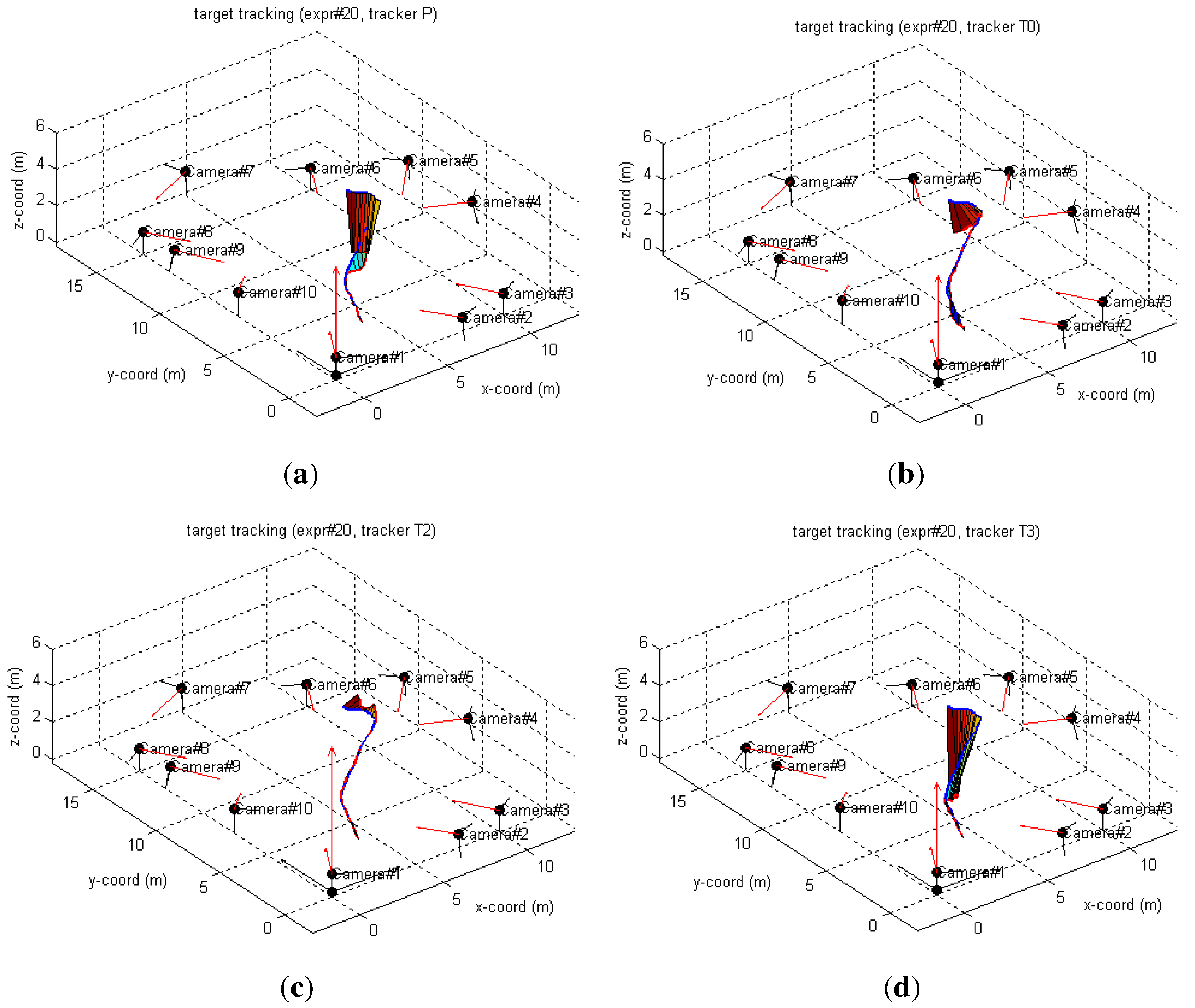
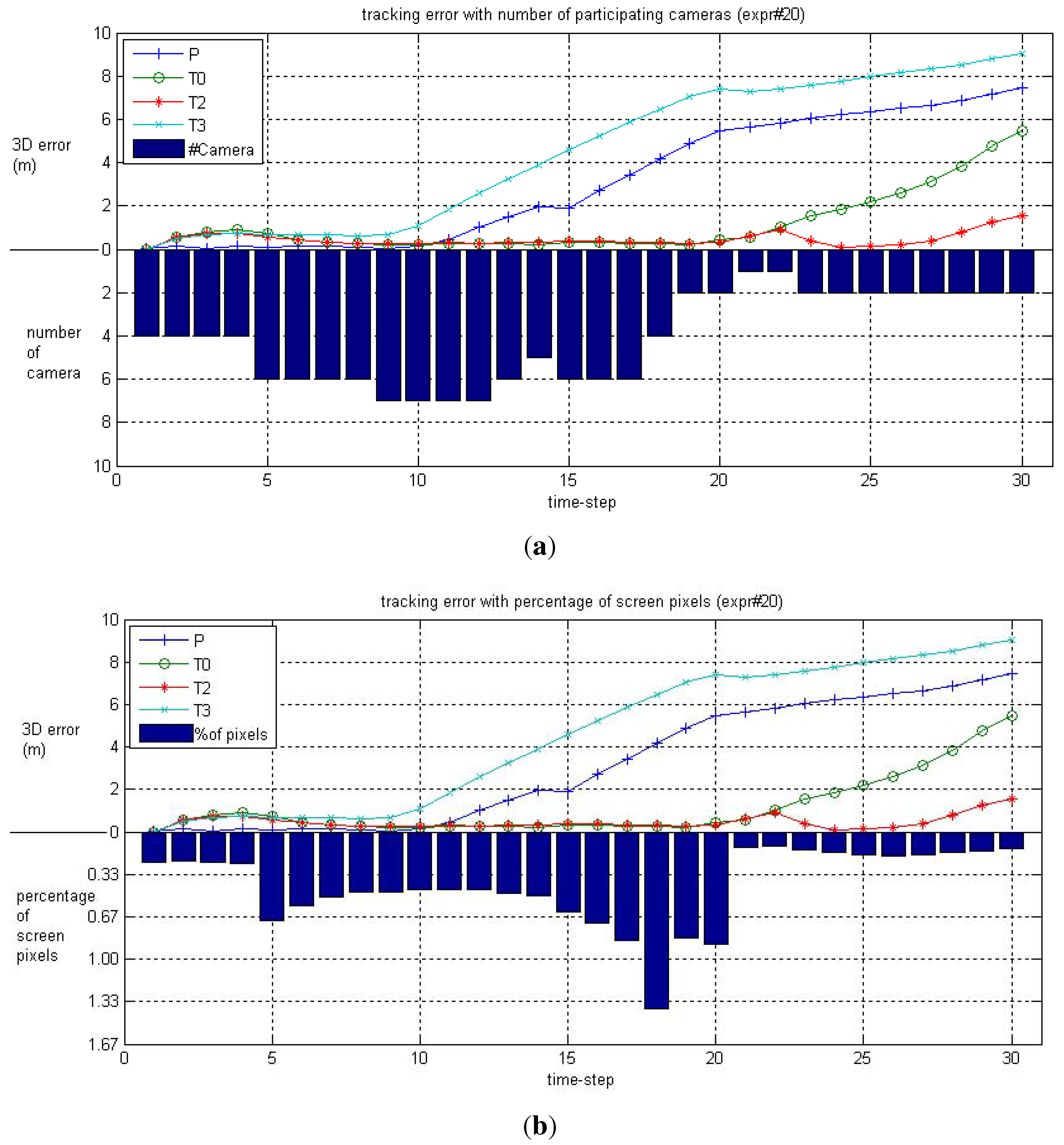
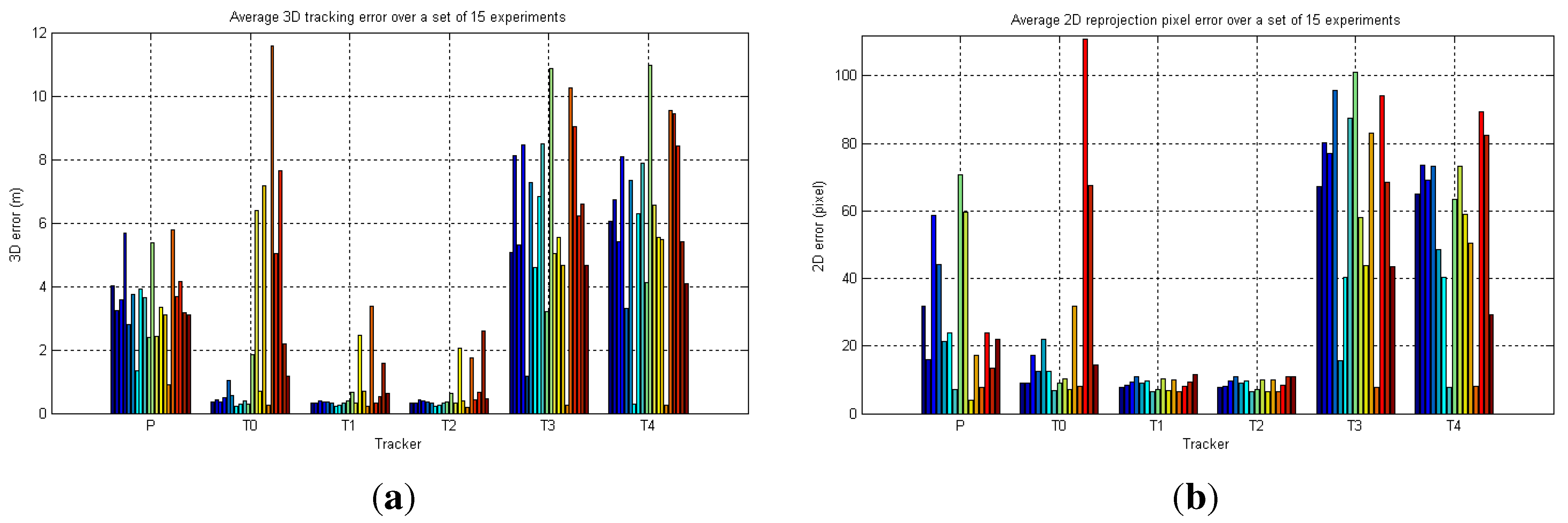
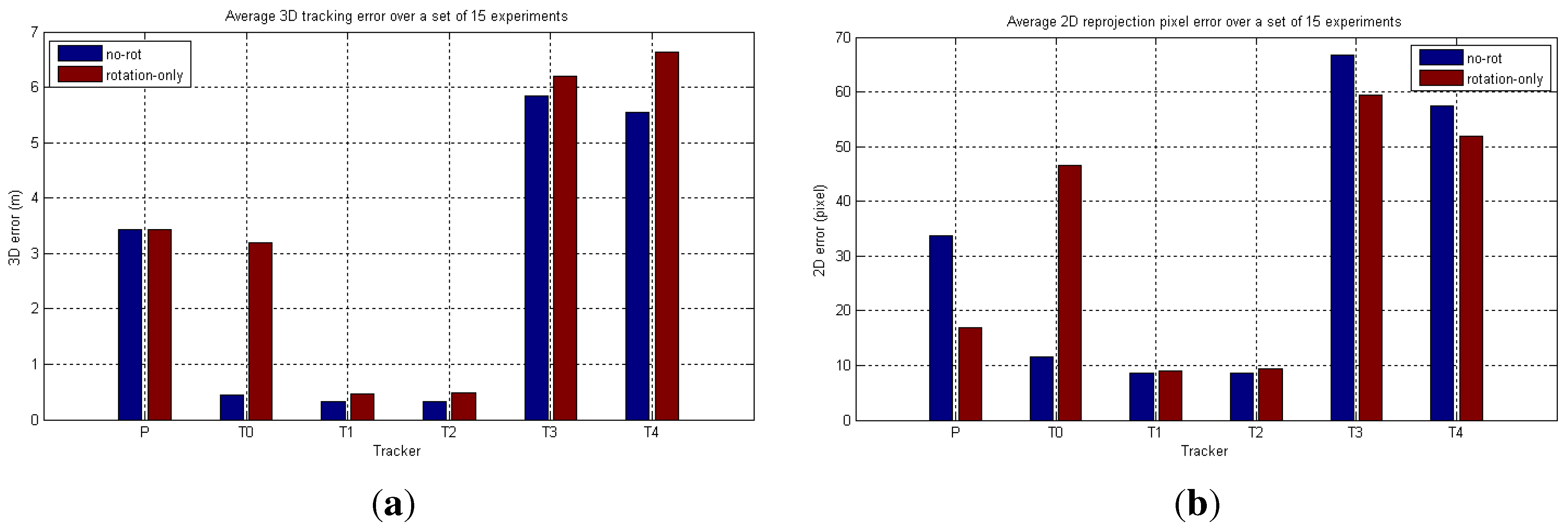
6. Performance Evaluation

In this section, we evaluate the proposed base tracker as well as trackers described earlier, and compare them with the tracker based on the 3D ray intersection method. We evaluate the trackers for four different camera network setups; two simulated camera networks and two real-world camera network deployments.

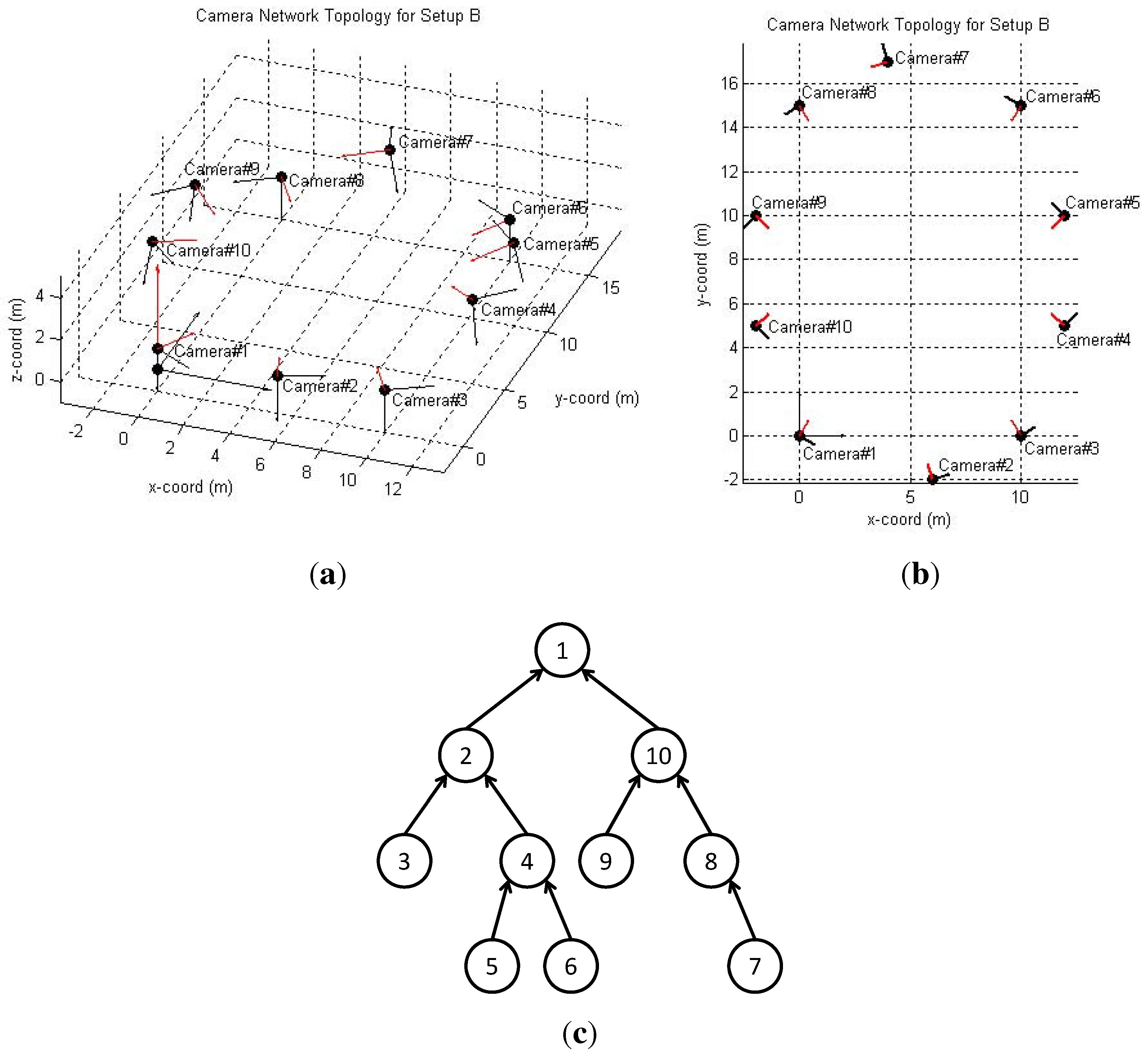
6.1. Simulated Camera Network

The scenarios considered here involve a wireless network of smart cameras arranged in a simulated topology. Setup B covers a much larger area as compared with setup A. The camera network setup consists of 10 cameras in a topology shown in Figure 6. We will see later that the optimal tracking approach depends on the camera topology, specifically tracker T3 performs better if the target is close to the camera and occupies a significant number of pixels in the camera images, while tracker T2 performs better if the target is farther away from the camera and occupies a very small number of pixels.

Figure 6. Camera network topology for setup B (a) 3D-view; (b) top-view; and (c) the routing tree.

Figure 6. Camera network topology for setup B (a) 3D-view; (b) top-view; and (c) the routing tree.

Synthetic Target A synthetic target with multiple colors moves in the 3D space, moving in and out of cameras field-of-view. Depending on the current target position and orientation, and the camera network geometry, the target’s projection on each camera image plane is computed and superimposed on a pre-recorded background video with visual clutter. The ellipsoid synthetic target is shown in Figure 7(a). As the target moves up and down a camera principle axis and rotates around its axis, the correct target projection with correct pixel color values is computed. Figure 7(b) shows the image captured by multiple cameras in setup A.

For each setup, we generated two types of simulated target trajectories, one when the target orientation is fixed and one when the target is rotating. Below, we present target tracking results for the simulated target and present a quantitative comparison of various trackers.

Figure 7. Synthetic target.

Figure 7. Synthetic target.

Simulated Camera Network Setup Figure 6 shows the simulated camera network setup B, which consists of 10 cameras. This setup covers a much larger area as compared with setup A. Figure 6(c) also shows the network routing tree for in-network aggregation as proposed in trackers T2 and T3.

Figure 8 shows the camera frames at all ten cameras at time-step 1, 10, 20 and 30 during the execution of tracker T2. Similar to camera network setup A, target initialization is performed manually at first time-step. The estimated target position is shown as a blue ellipse superimposed on camera frames. Unlike setup A, the target size in the image-plane for setup B is much smaller due to a much wider coverage. This results in a fewer number of pixels occupied by the target in each camera frame. A larger setup also means that the target will not remain visible in any given camera field-of-view for a large number of time-steps.

Figure 8. Camera images with estimated target state as blue ellipse for tracker T2.

Figure 8. Camera images with estimated target state as blue ellipse for tracker T2.

Figure 9(a)–Figure 9(d) show the 3D tracking result for trackers P, T0, T2 and T3, respectively (tracker T1 had similar performance as T2, while tracker T4 had similar performance as T3). The figures show the tracking performance as a patch graph, where the blue edge of the patch is the ground truth trajectory, while the red edge of the patch is the estimated target trajectory. The filled patches between the two edges represent the 3D tracking error at each time-step. As the target moves in the sensing region, it comes in and out of the fields-of-view of different cameras. Figure 10(a) shows the 3D tracking errors with the number of cameras that contain the target in their camera field-of-view (called participating cameras). At the beginning of the experiment, there are 4 cameras that can see the target. It drops to a single camera at time-step 21, with one more camera picking up the target at time-step 23. The top part of the figure shows the 3D tracking errors for the four approaches. Both trackers T0 and T2 performed quite well till time-step 21, when both of them started diverging because of a single participating camera. Unlike tracker T0, tracker T2 converged back to the ground truth as soon as there was one more participating camera. Trackers P and T3 performed poorly, even in the presence of as many as six participating cameras. This is explained in Figure 10(b), which shows the 3D tracking errors with the percentage of image pixels occupied by the target averaged over the number of participating cameras. As we can see, almost at all time-steps the percentage of image pixels is below 1% of the total pixels, i.e., the target occupied less than 800 pixels in a QVGA ($320\times 240$) image (equivalent of a circular region of radius 16 pixels). Since both trackers P and T3 are based on image-plane filtering, they fared poorly due to a fewer number of usable pixels.

Figure 9. Target tracking performance as a patch graph for (a) tracker P; (b) tracker T0; (c) tracker T2; and (d) tracker T3.

Figure 9. Target tracking performance as a patch graph for (a) tracker P; (b) tracker T0; (c) tracker T2; and (d) tracker T3.

Figure 10. 3D tracking errors for trackers P, T0, T2, and T3 with (a) number of participating cameras; and (b) percentage of image pixels occupied by the target.

Figure 10. 3D tracking errors for trackers P, T0, T2, and T3 with (a) number of participating cameras; and (b) percentage of image pixels occupied by the target.

Figure 11(a) and Figure 11(b) show quantitative evaluation of different trackers for setup B over a set of 15 simulated experiments. Of these 15 experiments, the target orientation is fixed for the first 10 experiments, whereas the target is rotating for the next 5 experiments. Figure 11(a) and Figure 11(b) show the average 3D tracking errors and the average 2D pixel reprojection errors for all the trackers. Figure 12(a) and Figure 12(b) show the average 3D tracking errors and the average 2D pixel reprojection errors for the rotating and non-rotating targets. It seems that target rotation does decrease the performance in 3D tracking by a small amount, while it does not have any significant bearing on the 2D pixel reprojection error.

Figure 11. Quantitative comparison of trackers for setup B over a set of 15 simulated experiments, (a) average 3D tracking error; and (b) average 2D pixel reprojection error.

Figure 11. Quantitative comparison of trackers for setup B over a set of 15 simulated experiments, (a) average 3D tracking error; and (b) average 2D pixel reprojection error.

Figure 12. Quantitative comparison of all trackers for setup B for rotating and non-rotating targets, (a) average 3D tracking error; and (b) average 2D pixel reprojection error.

Figure 12. Quantitative comparison of all trackers for setup B for rotating and non-rotating targets, (a) average 3D tracking error; and (b) average 2D pixel reprojection error.

Figure 13(a) and Figure 13(b) show the average 3D tracking error and the average 2D pixel reprojection error for all the trackers averaged over all experiments. The trend is the same for both of them. Trackers based on 3D kernel density, namely trackers T1 and T2, perform far better than any other tracker followed by the base tracker T0. The trackers based on image-plane filtering, namely trackers P, T3 and T4, perform poorly for this setup, due to the reasons mentioned above. In-network aggregation does not have any significant bearing on either the 3D kernel density based trackers or the image-plane based trackers.

Figure 13. Quantitative comparison of all trackers for setup B averaged over the set of 15 simulated experiments, (a) average 3D tracking error; and (b) average 2D pixel reprojection error.

Figure 13. Quantitative comparison of all trackers for setup B averaged over the set of 15 simulated experiments, (a) average 3D tracking error; and (b) average 2D pixel reprojection error.

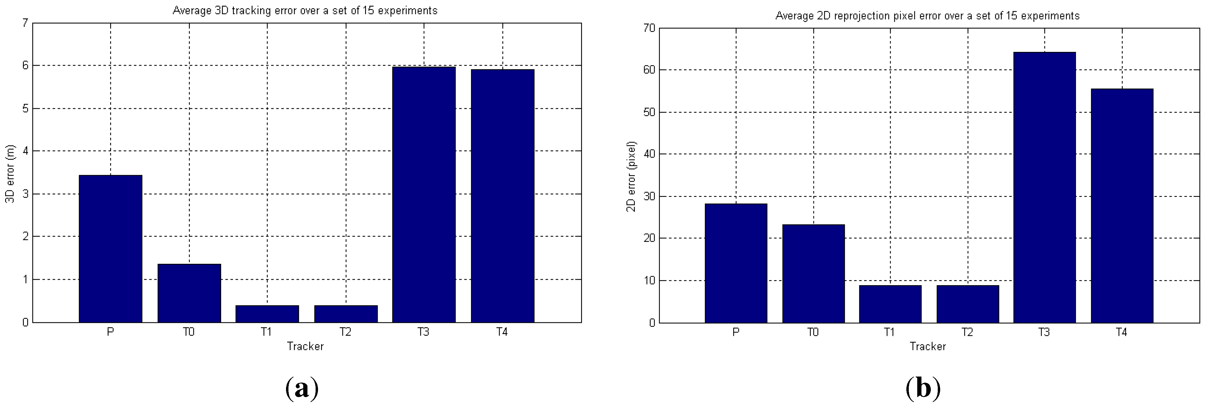
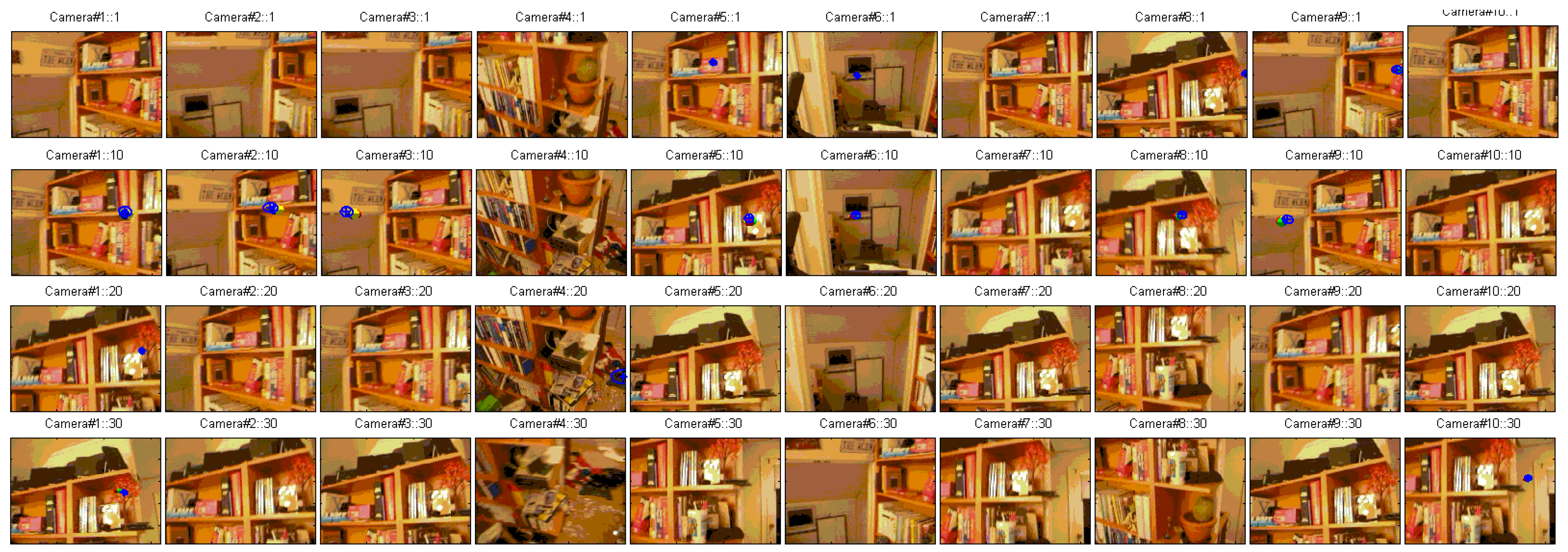
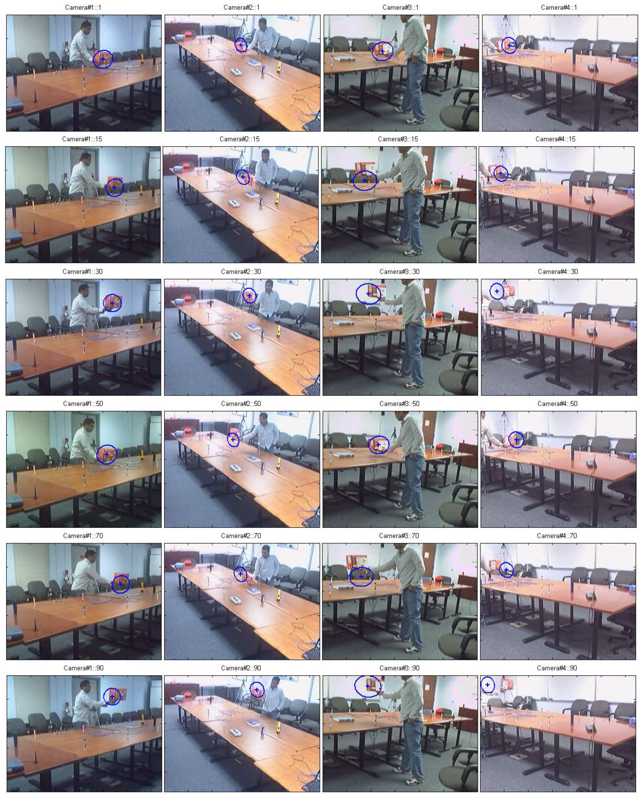
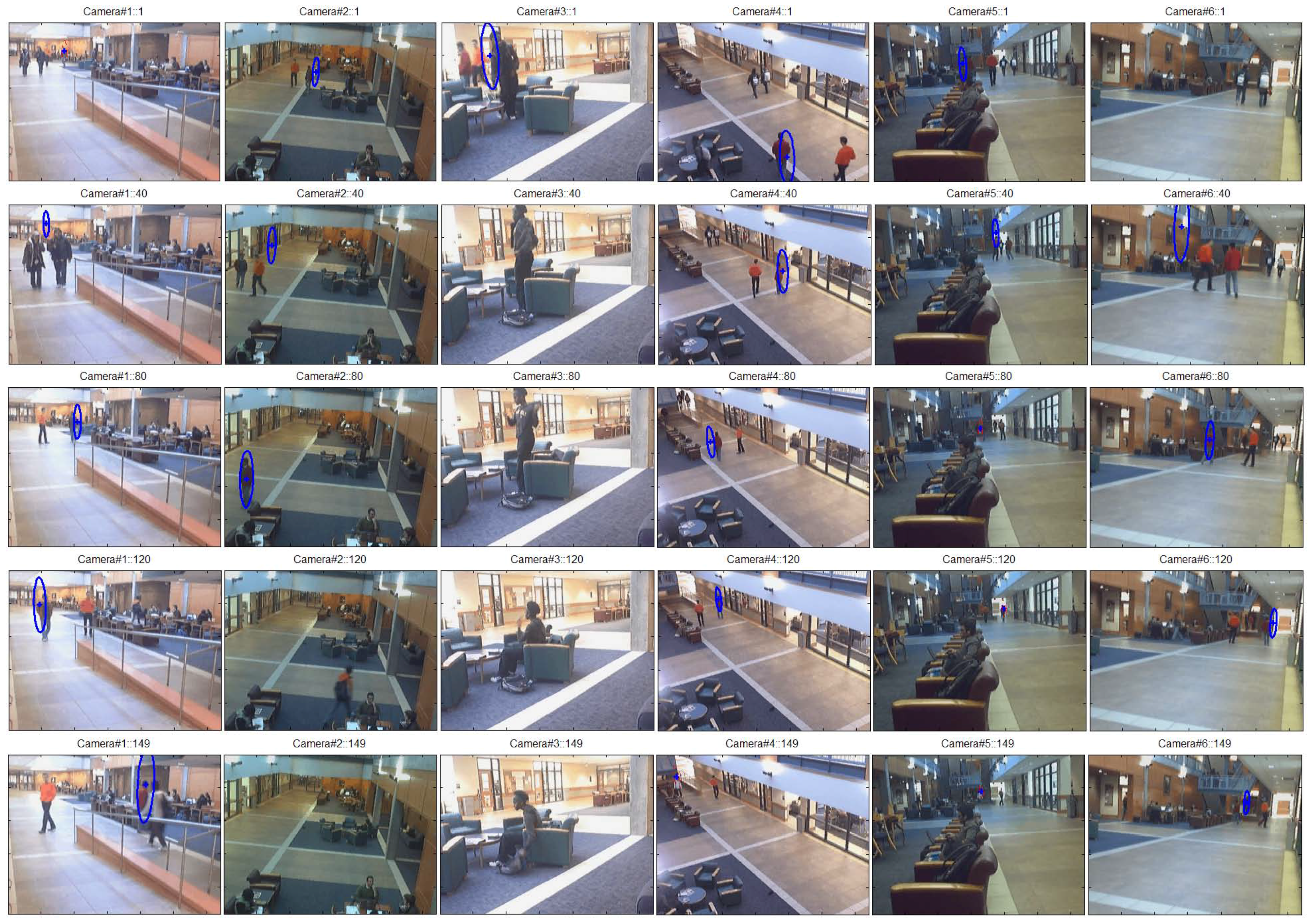
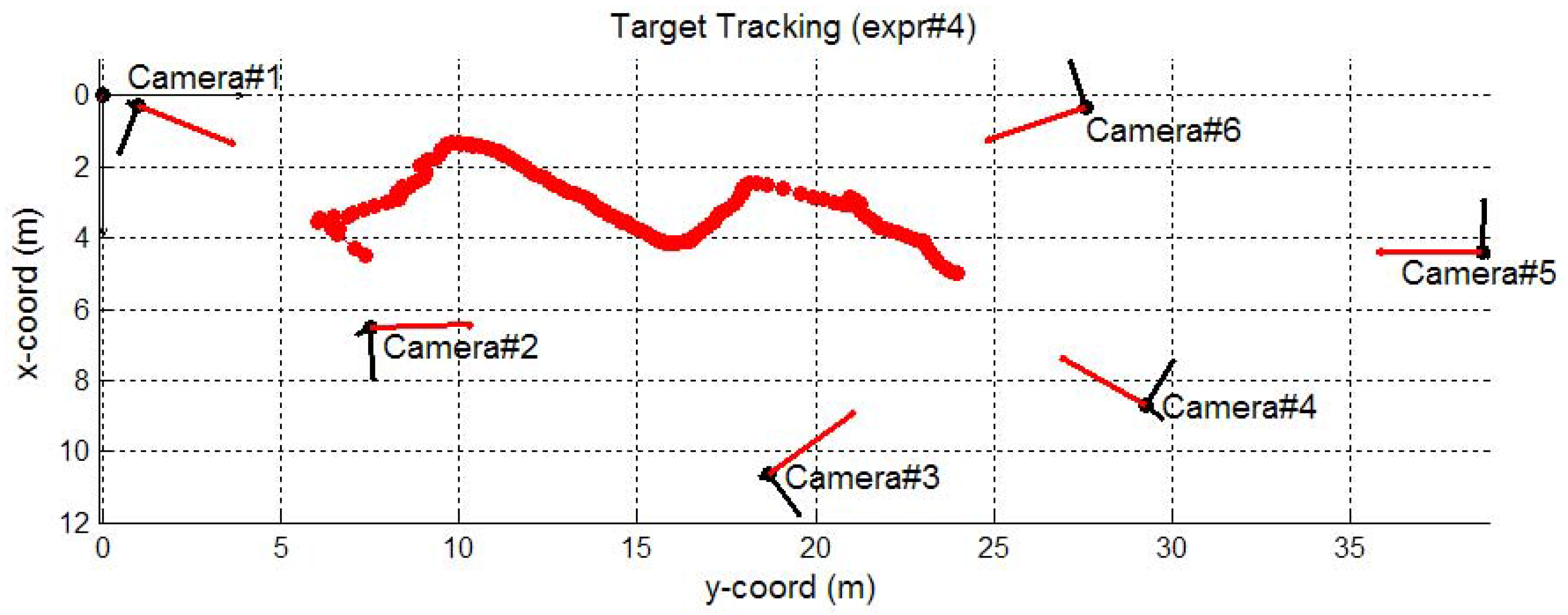
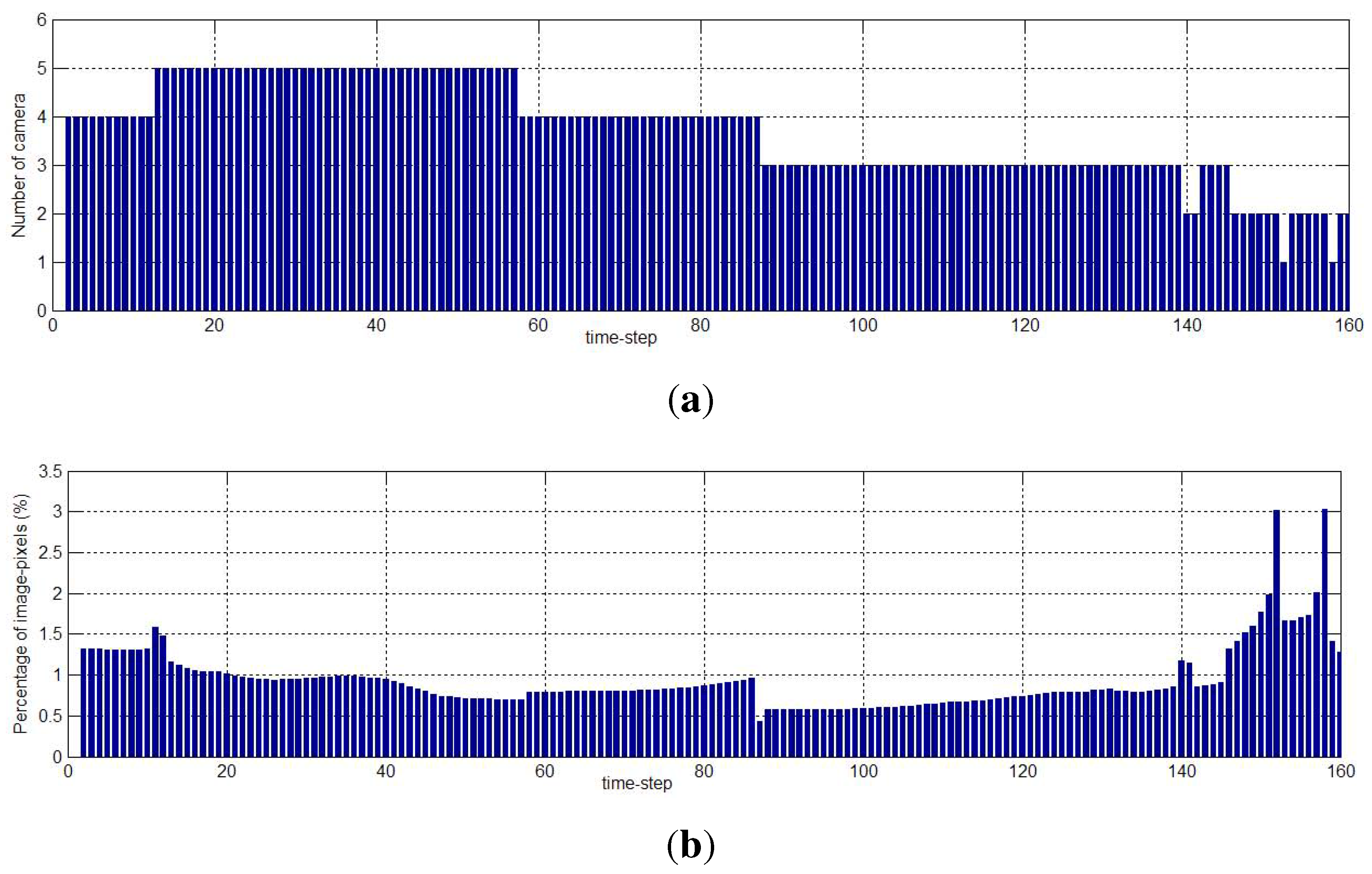
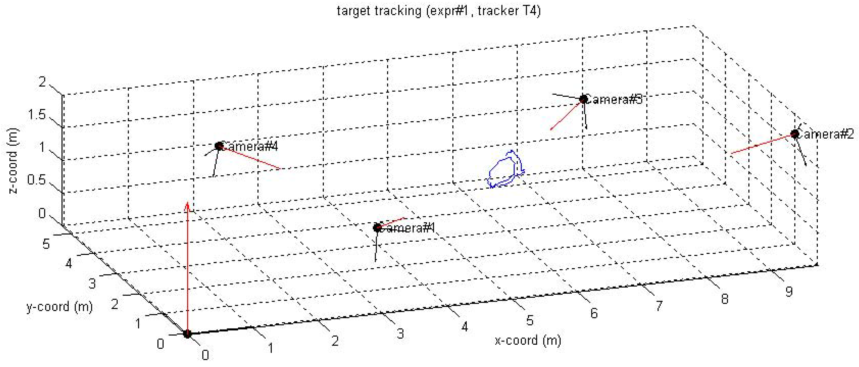
6.2. Real-World Camera Network

6.2.1. LCR Experiments

In this subsection, we present results for a real camera network deployment inside a Large Conference Room (LCR setup). The setup consists of 4 camera nodes in a topology as shown in Figure 14. A real target, in this case a typical box, is moved in the 3D space, moving in and out of coverage of cameras. Figure 14(c) also shows the network routing tree for in-network aggregation as proposed in trackers T2 and T3.

Figure 14. Camera network topology—LCR setup (a) 3D-view; (b) top-view; and (c) the routing tree.

Figure 14. Camera network topology—LCR setup (a) 3D-view; (b) top-view; and (c) the routing tree.

Figure 15 shows the camera frames at the four cameras at time-step 1, 15, 30, 50, 70 and 90 during the execution of tracker T3. Target initialization is performed manually at the first time-step. The estimated target positions are shown as blue ellipses superimposed on the camera frames. Figure 16 shows the 3D target trajectory as estimated by the tracker. In this experiment, as in all other experiments for this setup, the moving target was in the fields-of-view of four cameras.

Figure 15. Video target tracking using tracker T3 for experiment#1 for LCR setup.

Figure 15. Video target tracking using tracker T3 for experiment#1 for LCR setup.

Figure 16. Estimated target trajectory shown with camera network topology.

Figure 16. Estimated target trajectory shown with camera network topology.

Figure 17 shows the percentage of image pixels occupied by the target averaged over the number of participating cameras. As we can see, at all time-steps the percentage of image pixels is above 1% of the total pixels. This is perhaps the reason why tracker T3, which is based on image-plane filtering, works fine.

Figure 17. Average fraction of image pixels occupied by the target.

Figure 17. Average fraction of image pixels occupied by the target.

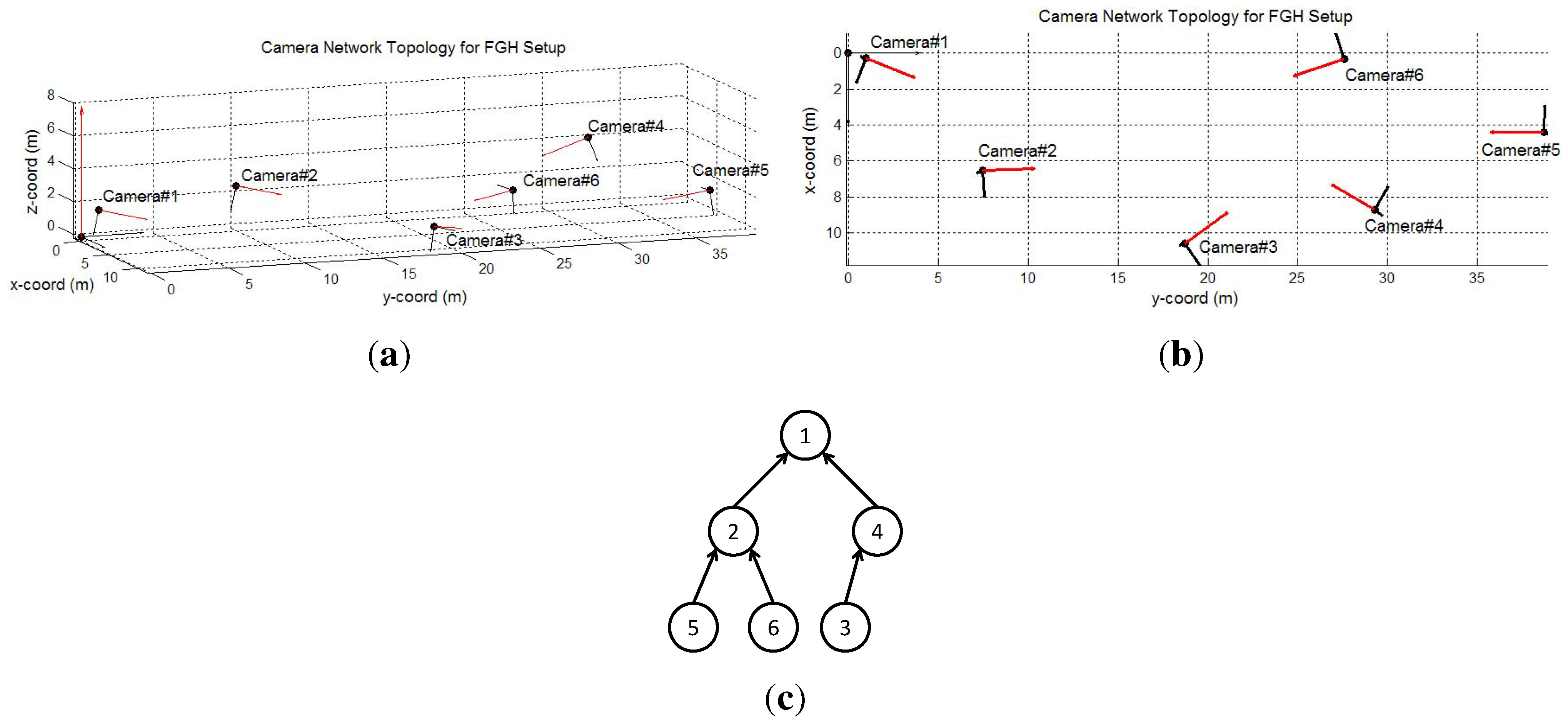
6.2.2. FGH Experiments

In this subsection, we present results for a real camera network deployment inside our department building (FGH). The setup consists of 6 camera nodes as shown in Figure 18. Figure 18(c) shows the network routing tree for in-network aggregation. We use OpenBrick-E Linux PCs with 533 MHz CPU, 128 MB RAM, an 802.11b wireless adapter, and QuickCam Pro 4000 as video sensors. The QuickCam Pro supports up to 640 × 480 pixel resolution and up to 30 Hz frame rate. Currently, the cameras record the videos at 4 Hz and 320 × 240 resolution and tracking is performed offline using a MATLAB implementation that realizes the tracker presented in Section 5.2 following the in-network aggregation scheme. Camera positions are measured manually and camera rotation matrices are estimated using known landmark points in the camera field-of-view. The targets to be tracked are the people moving in the FGH atrium, and target initialization is performed manually at the first time-step. Target model is learned a priori using a set of images of the target taken from multiple viewpoints. We chose 26 roughly equidistant viewpoints to cover the target from all sides with sufficient overlap between adjacent views. A detailed evaluation of the trackers as well as several other variations can be found in [38].

Figure 19 shows the camera frames at all six cameras at time-step 1, 40, 80, 120, and 150 during the execution of the tracker. The estimated target positions are shown as blue ellipses superimposed on the camera frames. This experiment demonstrates that even for an extended number of frames (160 frames) the tracker is successfully able to follow the target. During the length of this experiment, the target dramatically changes scale in camera images, comes in and out of different camera field-of-view, and is occluded by other people walking in the atrium. This experiment demonstrates the effectiveness of a 3D tracker over state-of-the-art 2D trackers by: (1) not having to learn or update the target model even in case of dramatic scale change and target rotation; and (2) not having to reinitialize a target when it (re-)enters a camera field-of-view. This experiment also demonstrates robustness of the tracker in the presence of target occlusion. Since we are using discriminatory features, i.e., color and texture, and we are performing tracking in 3D space, our tracker is successfully able to handle such occlusions.

Figure 18. Camera network topology—FGH setup (a) 3D-view; (b) top-view; and (c) network routing tree.

Figure 18. Camera network topology—FGH setup (a) 3D-view; (b) top-view; and (c) network routing tree.

Figure 19. Video target tracking at FGH.

Figure 19. Video target tracking at FGH.

Figure 20 shows the 3D target trajectory as estimated by the tracker. Since the sensing region in this setup is large, the target invariably moves in and out of the camera field-of-view. We have also put a threshold on the size of the projection of the target on the camera image plane. If the pixels occupied by the target in a particular camera image are below the threshold, we deem that frame unusable. Figure 21(a) shows the number of participating cameras at each time-step. At the beginning of the experiment, there are 3 cameras that participate in tracking, which grows to 5 participating cameras in the end. Figure 21(b) shows the percentage of image pixels occupied by the target averaged over the number of participating cameras. At all time-steps, the percentage of image pixels is below 1% of the total pixels. For more tracking results and videos we encourage the reader to go online at http://tinyurl.com/ya3xqrx and [38,39].

Figure 20. Estimated target trajectory shown with camera network topology.

Figure 20. Estimated target trajectory shown with camera network topology.

Figure 21. Number of participating cameras and average fraction of image pixels occupied by the target.

Figure 21. Number of participating cameras and average fraction of image pixels occupied by the target.

7. Conclusions

We present an approach for collaborative target tracking in 3D space using a wireless network of smart cameras. We model the targets in 3D space and thus circumvent the problems inherent in the tracker based on 2D target models. In addition, we use multiple visual features, specifically, color and texture to model the target. We propose a probabilistic 3D tracker and four variations of the tracker incurring different computational and communication cost, resulting in different tracking accuracy. We developed and implemented the trackers using sequential Monte Carlo methods. We provide a qualitative comparison of the trackers in terms of their Quality-of-Service (QoS), i.e., computational cost and communication cost, as well as their Quality-of-Information (QoI), i.e., the tracking accuracy. We also provided quantitative comparison of the trackers on a simulated network of smart cameras. The tracker variation with in-network aggregation provides the best tracking accuracy with low communication cost while preserving robustness against target size in image pixels. We evaluate the proposed tracker and the variations in a simulated camera network. Finally, we evaluate the proposed tracker for tracking people in a building using a 6-node camera network deployment. Although the experiments do not demonstrate multiple target tracking, we make the claim for multiple target-tracking because each individual target can be tracked by a completely separate 3D tracker, without any collaboration with other trackers. Since our 3D tracking approach is robust to occlusion, multiple targets occluding each other can be tracked by independent trackers. However, a collaborative suite of trackers can be envisioned to track multiple occluding targets and achieve better tracking accuracy than the independent trackers.

References

1. Rinner, B.; Winkler, T.; Schriebl, W.; Quaritsch, M.; Wolf, W. The Evolution from Single to Pervasive Smart Cameras. In Proceedings of the ACM/IEEE International Conference on Distributed Smart Cameras (ICDSC), Stanford, CA, USA, 7–11 September 2008.
2. Tyagi, A.; Keck, M.; Davis, J.; Potamianos, G. Kernel-Based 3D Tracking. In Proceedings of IEEE Workshop on Visual Surveillance, CVPR’07, Minneapolis, MN, USA, 22 June 2007.
3. Fleck, S.; Busch, F.; Straßer, W. Adaptive probabilistic tracking embedded in smart cameras for distributed surveillance in a 3D model. EURASIP J. Embedded Syst. 2007, 24. [Google Scholar]
4. Hu, W.; Tan, T.; Wang, L.; Maybank, S. A survey on visual surveillance of object motion and behaviors. Trans. Sys. Man Cyber Part C 2004, 34, 334–352. [Google Scholar]
5. Yilmaz, A.; Javed, O.; Shah, M. Object tracking: A survey. ACM Comput. Surv. 2006, 38. [Google Scholar] [CrossRef]
6. Toyama, K.; Krumm, J.; Brumitt, B.; Meyers, B. Wallflower: Principles and Practice of Background Maintenance. In Proceedings of the IEEE International Conference on Computer Vision, Kerkyra, Greece, 20–27 September 1999.
7. Ohba, K.; Ikeuchi, K.; Sato, Y. Appearance-based visual learning and object recognition with illumination invariance. Mach. Vision Appl. 2000, 12, 189–196. [Google Scholar]
8. Triesch, J.; von Der Malsburg, C. Democratic integration: Self-organized integration of adaptive cues. Neural Comput. 2001, 13, 2049–2074. [Google Scholar] [PubMed]
9. Hayman, E.; Eklundh, J.O. Probabilistic and Voting Approaches to Cue Integration for Figure-Ground Segmentation. In Proceedings of the 7th European Conference on Computer Vision-Part III, ECCV’02, Copenhagen, Denmark, 27 May–2 June 2002; pp. 469–486.
10. Canny, J. A computational approach to edge detection. IEEE Trans. Pattern Anal. Mach. Intell. 1986, 8, 679–698. [Google Scholar] [PubMed]
11. Moravec, H. Visual Mapping by a Robot Rover. In Proceedings of the 6th International Joint Conference on Artificial Intelligence, Tokyo, Japan, 20–23 August 1979; pp. 599–601.
12. Harris, C.; Stephens, M. A Combined Corner and Edge Detection. In Proceedings of the Fourth Alvey Vision Conference, Manchester, UK, September 1988; pp. 147–151.
13. Horn, B.K.P.; Schunck, B.G. Determining optical flow. Artif. Intell. 1981, 17, 185–203. [Google Scholar] [CrossRef]
14. Arulampalam, M.S.; Maskell, S.; Gordon, N. A tutorial on particle filters for on-line non-linear/non-Gaussian Bayesian tracking. IEEE Trans. Signal Process. 2002, 50, 174–188. [Google Scholar] [CrossRef]
15. Bar-Shalom, Y. Tracking and Data Association; Academic Press Professional, Inc.: San Diego, CA, USA, 1987. [Google Scholar]
16. Reid, D. An algorithm for tracking multiple targets. IEEE Trans. Autom. Control 1979, 24, 843–854. [Google Scholar] [CrossRef]
17. Birchfield, S. Elliptical Head Tracking Using Intensity Gradients and Color Histograms. In Proceedings of the IEEE Conference on Computer Vision and Pattern Recognition, Santa Barbara, CA, USA, 23–25 June 1998; pp. 232–237.
18. Comaniciu, D.; Meer, P.; Member, S. Mean shift: A robust approach toward feature space analysis. IEEE Trans. Pattern Anal. Mach. Intell. 2002, 24, 603–619. [Google Scholar] [CrossRef]
19. Comaniciu, D.; Ramesh, V.; Meer, P. Kernel-based object tracking. IEEE Trans. Pattern Anal. Mach. Intell. 2003, 25, 564–577. [Google Scholar] [CrossRef]
20. Tao, H.; Sawhney, H.; Kumar, R. Object tracking with Bayesian estimation of dynamic layer representations. IEEE Trans. Pattern Anal. Mach. Intell. 2002, 24, 75–89. [Google Scholar] [CrossRef]
21. Isard, M.; MacCormick, J. BraMBLe: A Bayesian Multiple-blob Tracker. In Proceedings of Eighth IEEE International Conference on the Computer Vision, ICCV 2001, Vancouver, BC, Canada, 7–14 July 2001; Volume 2, pp. 34–41.
22. Pérez, P.; Hue, C.; Vermaak, J.; Gangnet, M. Color-Based Probabilistic Tracking. In Proceedings of the 7th European Conference on Computer Vision, ECCV’02, Copenhagen, Denmark, 28–31 May 2002.
23. Quaritsch, M.; Kreuzthaler, M.; Rinner, B.; Bischof, H.; Strobl, B. Autonomous multicamera tracking on embedded smart cameras. EURASIP J. Embedded Syst. 2007, 2007, 35–35. [Google Scholar]
24. Shirmohammadi, B.; Taylor, C.J. Distributed Target Tracking Using Self Localizing Smart Camera Networks. In Proceedings of the Fourth ACM/IEEE International Conference on Distributed Smart Cameras, Atlanta, GA, USA, September 2010; pp. 17–24.
25. Focken, D.; Stiefelhagen, R. Towards Vision-Based 3-D People Tracking in a Smart Room. In Proceedings of the Fourth IEEE International Conference on Multimodal Interfaces, Pittsburgh, PA, USA, 14–16 October 2002.
26. Mittal, A.; Davis, L.S. M2Tracker: A multi-view approach to segmenting and tracking people in a cluttered scene. Int. J. Comput. Vis. 2003, 51, 189–203. [Google Scholar] [CrossRef]
27. Soto, C.; Song, B.; Chowdhury, A.K.R. Distributed Multi-Target Tracking in a Self-Configuring Camera Network. In Proceedings of the IEEE Conference on Computer Vision and Pattern Recognition, Miami, FL, USA, 20–25 June 2009; pp. 1486–1493.
28. Fleuret, F.; Berclaz, J.; Lengagne, R.; Fua, P. Multicamera people tracking with a probabilistic occupancy map. IEEE Trans. Pattern Anal. Mach. Intell. 2008, 30, 267–282. [Google Scholar] [CrossRef] [PubMed]
29. Berclaz, J.; Shahrokni, A.; Fleuret, F.; Ferryman, J.; Fua, P. Evaluation of Probabilistic Occupancy Map People Detection for Surveillance Systems. In Proceedings of the IEEE International Workshop on Performance Evaluation of Tracking and Surveillance, Miami, FL, USA, 20–25 June 2009.
30. Leibe, B.; Cornelis, N.; Cornelis, K.; van Gool, L. Dynamic 3D Scene Analysis from a Moving Vehicle. In Proceedings of the IEEE Conference on Computer Vision and Pattern Recognition, CVPR’07, Minneapolis, MN, USA, 17–22 June 2007.
31. Gandhi, T.; Trivedi, M.M. Person tracking and reidentification: Introducing Panoramic Appearance Map (PAM) for feature representation. Mach. Vision Appl. 2007, 18, 207–220. [Google Scholar] [CrossRef]
32. Gandhi, T.; Trivedi, M.M. Panoramic Appearance Map (PAM) for Multi-Camera Based Person Re-Identification. In Proceedings of the IEEE Conference on Advanced Video and Signal Based Surveillance, Sydney, NSW, Australia, 22–24 November 2006.
33. Ojala, T.; Pietikäinen, M.; Mäenpää, T. Multiresolution gray-scale and rotation invariant texture classification with local binary patterns. IEEE Trans. Pattern Anal. Mach. Intell. 2002, 24, 971–987. [Google Scholar] [CrossRef]
34. Kuipers, J.B. Quaternions and Rotation Sequences: A Primer with Applications to Orbits, Aerospace and Virtual Reality; Princeton University Press: Princeton, NJ, USA, 2002. [Google Scholar]
35. Tron, R.; Vidal, R.; Terzis, A. Distributed Pose Averaging in Camera Networks via Consensus on SE(3). In Proceedings of the Second ACM/IEEE International Conference on Distributed Smart Cameras, ICDSC 2008, Stanford, CA, USA, 7–11 September 2008.
36. Brown, R.G.; Hwang, P.Y.C. Introduction to Random Signals and Applied Kalman Filtering with Matlab Exercises and Solutions; John Wiley & Sons: Hoboken, NJ, USA, 1996; Chapter 8. [Google Scholar]
37. Bilmes, J. A Gentle Tutorial of the EM Algorithm and Its Application to Parameter Estimation for Gaussian Mixture and Hidden Markov Models; Technical Report TR-97-021; International Computer Science Institute: Berkeley, CA, USA, April 1998. [Google Scholar]
38. Kushwaha, M. Feature-Level Information Fusion Methods for Urban Surveillance Using Heterogeneous Sensor Networks. Ph.D. Thesis, Vanderbilt University, Nashville, TN, USA, 2010. [Google Scholar]
39. Kushwaha, M.; Koutsoukos, X. 3D Target Tracking in Distributed Smart Camera Networks with In-Network Aggregation. In Proceedings of the Fourth ACM/IEEE International Conference on Distributed Smart Cameras, Atlanta, GA, USA, September 2010; pp. 25–32.