Design Issues in Constructing Chain Oriented Logical Topology for Wireless Sensor Networks and a Solution

Abstract

An optimised logical topology facilitates the sensors of a network to communicate with each other with little overheads, lower energy consumption, and reduced latency. It also lengthens the lifetime of the network, provides scalability, and increases reliability in communications. However, designing an optimal logical topology for wireless sensor networks requires considering numerous factors. In this paper, we elaborately discuss these design issues and challenges. We also present a chain oriented logical topology, which offers solutions to those design issues. The proposed logical topology provides not only a communication abstraction, but also node management and resource management. The performance of the proposed topology is compared with other topologies with respect to energy consumptions, latency, and lifetime of the network.

1. Introduction

Wireless sensor networks (WSNs) are formed by a large collection of power-conscious wireless-capable sensors without the support of pre-existing infrastructure, possibly by unplanned deployment. With the sheer number of sensor nodes, their unattended deployment and hostile environment very often preclude reliance on physical configuration or physical topology. It is, therefore, often necessary to depend on the logical topology.

The logical topology of a wireless sensor network is formed by the communication graph of the network. A communication graph of a WSN is an undirected graph $G=(V,E)$ where V denotes the sensors deployed, and E denotes the available communication links among the sensor nodes. As logical topology inherently defines the type of routing paths, indicates whether to use broadcast or unicast, and determines the sizes and types of packets and other overheads, choosing the right topology helps to reduce the amount of communication needed for a particular problem. Thus energy can be saved. An efficient topology, which ensures that neighbours are at a minimal distance, reduces the probability of message being lost between sensors. A topology can also reduce the radio interference, thus reducing the waiting time for sensors to transmit data [1,2,3]. Moreover, topology facilitates data aggregation, which greatly reduces the amount of processing cycles and energy, resulting in a longer lifetime for the network [4,5]. In addition, topology inherently defines the size of a group, how to manage new members in a group, and how to deal with members who have left the group. With the awareness of the underlying network topology, more efficient routing or broadcasting schemes can be achieved. Furthermore, the network topology in WSNs can be changed by varying the nodes’ transmitting ranges and also by adjusting the wake/sleep schedule of the nodes [6,7]. Therefore, more energy can be saved if the network topology is maintained in an optimal manner.

Additionally, much research has taken place to justify the performance of different logical topologies [8,9,10,11]. Chain oriented topology has been identified as being more promising than other topologies of WSNs [12,13,14,15,16,17,18]. Chain oriented topologies minimise many of the constraints of WSNs. For example, energy consumptions by the sensor nodes can be greatly reduced by the chain oriented topology [19,20,21,22]. For data fusion/aggregation, chain oriented topology offers substantial advantages due to the logical structure of the sensor nodes [23,24]. It is also possible to obtain collision-free transmissions using a chain oriented topology [25]. Other WSNs requirements, such as connectivity, robustness, scalability, responsiveness, and reliability, can also be enhanced by chain oriented topologies.

To achieve the abovementioned outcomes, the careful design of chain oriented topology is essential. Designing a logical topology for WSNs needs to be considered from different perspectives, namely: (i) resource oriented considerations, such as energy consumption and time requirement; (ii) networking related considerations, such as connectivity, robustness, and reliability; (iii) data centric considerations, such as data collection strategies and data aggregation facilities; (iv) architecture oriented considerations, such as scalability, task orientation, and light weighting; and (v) Network management considerations, such as fault detection and performance management. The drawbacks of chain oriented topologies, such as latency, also need to be considered. In this paper, we propose a variant of chain oriented logical topology. The main aim of this study is to design a logical topology, so that the proposed topology retains the advantages of the chain oriented topologies, and at the same time, overcomes the problems of the chain oriented topology. In designing the proposed logical topology, we considered all the aspects discussed above.

It should be noted that logical topology problems are sometimes confused with routing problems in WSNs. Our aim was not to design a routing protocol, but to construct a logical topology for WSNs. Although logical topologies of wireless networks inherently define routing paths, the problem is not limited to delivering data from the source to the destination node(s). The logical topology designs the logical structure, and provides the communication abstraction, while routing protocols can be established on the basis of the logical abstraction. Moreover, we aim to design a logical structure of deployed sensors, with which other protocols (e.g., data dissemination or data collection protocols, time synchronization protocols, event synchronization protocols and other different application protocols) can be designed.

The paper is organised as follows. Section 2 discusses the issues related to logical topology design. Section 3 describes the existing chain oriented topologies and discusses the observations of different chain oriented topologies. Section 4 presents a detailed description of the proposed topology and defines the different terminologies used. Section 4 also discusses issues regarding topology designs, the workflow and the communication abstraction of the proposed topology. Section 5 discusses network management issues for the proposed topology while Section 6 evaluates the performance of the proposed topology, with conclusion presented in Section 7.

2. Issues in Topology Design

This section provides detailed descriptions of different design aspects that should be considered in constructing the proposed logical topology.

2.1. Hierarchical Structure

The first issue to consider in designing the proposed logical topology is the structure of the topology, i.e., whether the topology should have a hierarchical-structured or not. A hierarchical structure has many advantages over a non-hierarchical structure. For example, a hierarchical network structure can reduce the length of time for transmitting messages between two distant nodes in a sensor network. The structure requires that some capable sensors act as local leaders/clusterheads to interface with the outside world. Additionally, the grouping/clustering of sensors can also aggregate and process data locally to reduce communication load in the network. However, this solution may not be energy efficient. It is well known that, given two nodes, the radio transmission power required at the transmitter end is exponentially proportional to the distance from the receiver [26]. For hierarchical structures, leaders/clusterheads need to use exponentially more power to relay messages because they decrease the number of intermediate nodes, and consequently have to deal with longer distances. Although a hierarchical structure is not theoretically energy efficient, it is an advantageous choice for a large-scaled dense sensor networks for several reasons. The exponential effect is not significant as the distances within a dense environment are limited. Furthermore, by careful rotation of leaders/clusterheads, a balanced energy dissipation state can be achieved, where some sensors can afford to consume more energy. In contrast, multi-hop communication without a hierarchical structure consumes energy among all participant sensors in an unplanned way, resulting in faster energy exhaustion of sensors with lower energy capacity. With local leaders/clusterheads taking more responsibility, energy can be saved for energy-constrained sensors, which extends the lifetime of the overall network. For this reason, we choose hierarchical structure for the proposed topology.

2.2. Resource Oriented Considerations

Designing topology for resource-constrained sensor network requires careful consideration regarding the consumption of resources such as energy, time, processing capability, and memory requirements. Obviously, the first consideration should be energy. [27,28] have shown that chain oriented topology greatly reduces energy consumption, and thus this section will not attempt to compare the consumption of energy and other resources within different topologies that has already been reviewed. This section, however, will focus on areas of resource utilization within chain oriented topology that can be further improved.

The aim of the resource oriented consideration is not only to save energy but also to ensure that energy dissipation is evenly distributed. As the chain leaders undertake more tasks and long distant communications, they deplete energy more rapidly compared with other nodes in the network. Thus, it is important to change the role of the leader regularly, so that the load of the leader is distributed among many nodes. Conversely, very frequent changing of the role of chain leaders can diminish the performance of chain oriented sensor networks. At the same time, energy consumption also increases, due to an increase in the number of control messages regarding the new leaders, and their selection procedures. Thus, determining the time to change the role of the leader is crucial.

Another important resource related issue is the time required by the network to perform an operational round. If the sensors of the network construct only one chain, latency becomes very high. This is because each sensor node needs to wait for the data from its predecessor node. This latency can be reduced by constructing multiple chains using the sensor nodes. Multiple chains in the network introduce parallelism, which directly recommends the use of multiple chains instead of a single chain. Multiple chains are advantageous compared with a single chain not only for decreasing the latency, but also for receiving other facilities, such as scalability, flexibility, and ease for management. For these reasons, we propose a topology that uses multiple chains instead of a single chain.

2.3. Networking Related Considerations

Connectivity, robustness, and reliability are the most important issues regarding networking related considerations. In sensor networks, one of the main concerns is that sensor nodes can die anytime, and because of wirelessness, the probability of missing a message is high. The topology should take care of the communication model whenever a sensor node dies or is not responding.

Connectivity, robustness, and reliability are directly related to the distance between two nodes that communicate wirelessly. For a pair of nodes with a short distance between them, higher values of connectivity, robustness, and reliability are achievable than in a pair of nodes having a longer distance. Therefore, it is advantageous to select the closest node as a neighbouring node along the chain. However, adopting the greedy method of choosing the nearest neighbour results in fewer longer links at the end of the chain formation phase. On the other hand, applying a brute-force search for searching neighbour nodes is not suitable for WSNs due to the scarcity of processing power and memory. Thus, while designing the chains for the proposed topology, we put emphasis on keeping the chains shorter in order to reduce time delays and memory complexities.

2.4. Data Related Considerations

WSNs are very much data oriented. Usually WSNs are deployed to collect environmental/monitoring data. Thus, data related considerations during the designing of the topology are crucial. The two most important issues of data related considerations are data collection and data aggregation, as considered below.

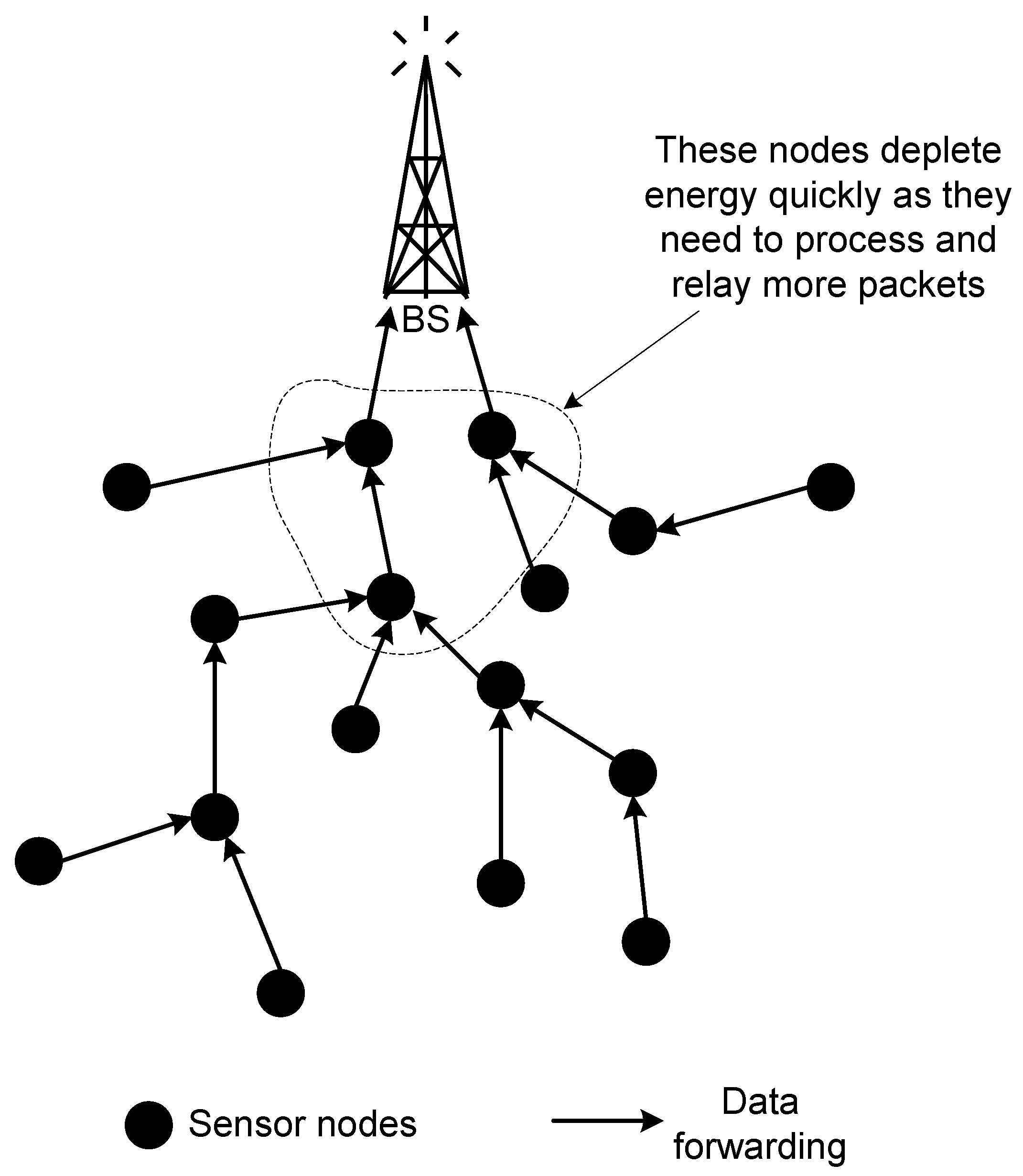
Data collection. According to the system model, based on which the multiple chain oriented logical topology is proposed, sensed data are continuously/periodically collected at all of the sensor nodes, and forwarded through wireless communications to a central base station (BS) for further processing. Sensor data collection requires that all sensing data are correctly and accurately collected and forwarded to the BS, as sometimes the complexity of the data requires global knowledge in order to be processed. This feature thus prevents the use of data aggregation/fusion techniques that are typically employed to enhance the network performance. As a result, the major traffic in sensor data collection is the reported data from each sensor to the BS. Such a “many-to-one" traffic pattern, if not carefully handled, causes high unbalanced and inefficient energy consumption in the entire network. For example, [29] reports on the energy hole problem, where sensor nodes close to the BS are depleted quickly due to traffic relays and create a hole shape area that leaves the remaining network disconnected from the BS.

Figure 1 depicts an example of such a scenario. One possible solution to alleviate the issue of uneven energy dissipation is to avoid the construction of complex chains, where two or more nodes send their data to a single node. Another solution is to exclude the set of sensor nodes from performing the same task repeatedly.

Figure 1. Uneven energy dissipation by sensor nodes.

Figure 1. Uneven energy dissipation by sensor nodes.

Data aggregation. Besides considering the data collecting technique, another important issue to consider is data aggregation. The information gathered in a sensor network is highly correlated, due to a spatial and temporal correlation between successive measurements. Exploiting the data-centricity and the spatial-temporal correlation characteristics allows the application of effective in-network data aggregation techniques, which further improve the energy-efficiency of the communication in WSNs [30]. Aggregation can eliminate the inherent redundancy of the raw data collected as well as diminish the traffic in the network, thereby reducing congestion and induced collisions [31]. Thus, data aggregation policies are adopted in WSNs to increase the lifetime of the network. However, designing aggregation points for data aggregation requires careful attention. Data aggregating points consume more energy in processing the aggregation method, and unplanned, non-distributed aggregation points can drastically affect the lifetime of the network [32].

2.5. Architectural Related Considerations

The architecture of wireless sensor networks needs to accommodate the following three characteristics:

Scalability. Large-scale WSNs rely on thousands of tiny sensors to observe and influence the real world [33]. These sensors do not necessarily need to be active at all times, so sensors can be dynamically added to or removed from the network [34]. A durable and scalable architecture would allow responses to changes in the topology with minimum update messages being transmitted. Another important feature of chain oriented WSNs that affects scalability is the number of nodes in a chain. If there is a single chain in the whole network, the topology is subject to poor scalability. On the other hand, multiple chains in the network can solve the scalability problem. However, all the chains in the network should be of similar length. Therefore, in designing the proposed topology, we keep the lengths of multiple chains similar.

Task Orientation. The tasks of wireless sensor networks range from the simplest data capturing and static-nodes to the most difficult data collecting, mobile-node sensor network [33,35]. The sensor networks for different tasks may behave very differently. The software structure should be optimised and tailored toward a predefined task-set for each node. Thus, the proposed topology divides all the deployed nodes in the hierarchical structure, assigns specific tasks to each node, and provides a communication abstraction, through which other protocols can be designed.

Light Weighting. The computing and storage capabilities of sensor nodes are very limited. Lightweight operations, such as data aggregation, reduced message size, and a piggyback acknowledgment mechanism, must be applied to the architecture. In designing the communication abstraction of the proposed logical topology, we consider this notion.

2.6. Network Management Considerations

Large-scale wireless sensor networks are composed of hundreds or thousands of sensor nodes. For this reason, effective management of WSNs is a big challenge. Network management includes fault management, configuration management, security management, performance management, and accounting management [29]. In particular, most wireless sensor nodes are powered by battery rather than external power. Thus, energy conservation is a key issue for the design, implementation and management of WSNs.

Effective management requires a practical architecture that is optimised to the features of WSNs and satisfies the requirements of wireless network management protocol. Therefore, the logical topology is built in such a way that it can be used as the underlying architecture by the network management scheme. Once the architecture of the network management scheme is constructed, various components of network management scheme such as primitives, functionalities, and Management Information Base (MIB) can be designed easily. Since both the logical topology and the network management scheme use the same architecture, this phenomena can be used to assess a system’s resource requirements, response time, and performance patterns and anti-patterns with the help of a performance model [36].

3. Existing Chain Oriented Topologies

Chain oriented topologies have been used by researchers in designing various protocols, among which data broadcasting protocols, data collection/gathering protocols and routing protocols are the major instances. Chain topologies are mainly used in these protocols to reduce the total energy consumption, and thus to increase the lifetime of the network. This section discusses different protocols, which use chain oriented topologies.

Lindsey and Raghavendra present several chain oriented data broadcasting and data collection/gathering protocols for sensor networks [27,37]. They investigate broadcast problems in sensor networks and adopt a chain oriented approach for situation awareness systems, where networked sensors track critical events via coordination. They propose a linear-chain scheme for all-to-all broadcasting and data gathering. They also propose a binary-combining scheme for data gathering, which divides each communication round into levels in order to balance the energy dissipation in sensor networks. For broadcasting, the linear-chain scheme starts data transmission with a packet at the beginning of a chain. Each node along the chain attaches its own data to this packet. Eventually, information from the entire network reaches the end of the chain. The same procedure runs in the reverse direction to complete all-to-all broadcasting. The linear-chain scheme can also be applied to gather data in sensor networks. To gather data, each node senses and transfers information along the chain to reach one particular node that will send data to a remote BS. Such a scheme is named PEGASIS (Power-Efficient Gathering in Sensor Information Systems) [27].

PEGASIS is the first protocol that uses chain oriented topology for periodic data collection from the target field. PEGASIS forms a chain of the sensor nodes and uses this chain as the basis for data aggregation. In PEGASIS, the chain is formed using a greedy approach, starting from the node farthest to the sink. The nearest node to this is added as the next node in the chain. This procedure is continued until all the nodes are included in the chain. A node can be in the chain at only one position. Figure 2(a) shows the chain creation method. In this figure, the node $C0$ lies furthest from the BS. Chain construction starts from the node $C0$, which connects to the node $C1$ as $C1$ is the closest node to $C0$. The node $C1$ then connects to its closest node $C2$, and so on. In this fashion a chain $C0-C1-C2-C3-C4-C5$ is created. Figure 2(b) shows the data collection strategy adopted by PEGASIS. In the constructed chain, a leader node for each round is selected randomly. The authors argue that randomly selecting a head node is beneficial as nodes are more likely to die at random locations, thus providing robust network. All nodes send their data to the leader node, and then, the leader node sends the data to the BS. For example, in Figure 2(b), $C3$ is selected as the leader node. The node $C5$ passes its data to the leader node $C3$ via the node $C4$.

Figure 2. PEGASIS protocol chain. (a) chain formation using greedy method; (b) Data fusion at the leader node, and transmitting it to BS.

Figure 2. PEGASIS protocol chain. (a) chain formation using greedy method; (b) Data fusion at the leader node, and transmitting it to BS.

PEGASIS suffers from several problems. First, in this protocol the role of the leader node changes in every round of data collection. This causes extra overhead. Moreover, when a node is selected as the leader, the protocol considers neither the distance of the node from the BS nor its energy level. Additionally, the chain in PEGASIS is constructed by a greedy algorithm. Using this chain causes some problems, such as an unexpectedly long transmission time, and non-directional transmission to the BS. These problems adversely affect the energy efficiency of WSNs. All nodes in sensor networks transmit their data in order. Therefore, the delay increases linearly as the number of nodes increases. Thus, PEGASIS is not scalable for large-scale WSNs. PEGASIS also causes redundant transmission of data as a result of having a single leader.

To resolve the delay problem of PEGASIS, a 3-level PEGASIS was proposed. In 3-level PEGASIS, the chain is cut into several chains. Each chain has a leader that gathers data from its neighbours and sends aggregated data to the upper level leader. The delay may decrease with 3-level PEGASIS. However, 3-level PEGASIS raises the problem of wireless interference as it does not consider the relative location of nodes. Another problem is that unexpected long transmission may occur because the leader of a chain sends a packet to the upper leader or the sink node by one hop transmission.

Reference [38] provides an algorithm for constructing the energy efficient chain called the minimum total energy (MTE) chain. These chain construction algorithms use centralised approaches for constructing the chain and elect the leader node for transmitting data back to the sink by taking turns. However, if the remaining energy of each node is not taken into account in the leader election, the nodes with low remaining energy will easily run out of energy, leaving just a small number of survival nodes to perform the sensing task. From the viewpoint of network lifetime, this is not ideal.

Both PEGASIS and MTE approaches use centralised chain construction, which has a number of disadvantages. Firstly, their transmission cost calculation based on distance may not reflect the exact cost in different practical environments due to radio irregularity as indicated in [39]. Secondly, these centralised approaches may not scale well for large network or large number of nodes. Moreover, after some time, nodes far away from the sink easily run out of battery since they consume more energy to transmit to the sink as a leader.

Power Aware Chain (PAC) [19] addresses these issues by constructing the chain using a distributed algorithm. PAC is a chain oriented routing scheme, and here the distributed algorithm presented for constructing the routing chain is based on the minimum cost tree. In this protocol, the transmission cost is calculated based on the received signal strength between nodes. Therefore, it does not require global knowledge of nodes’ location information and provides more accurate communication cost calculation among nodes under different practical deployment environments. The proposed power aware mechanism for leader node election in the chain ensures more uniform energy consumption among nodes. Thus, in PAC, all nodes die at approximately the same time, which provides better active network operation time than the case where there are only a few nodes still functioning while almost all other nodes have died. However, the problem of PAC is that it constructs a single chain, which causes a delay in gathering data from all the sensor nodes of the network. This protocol also requires very high processing complexity for a large network, and thus is not applicable for a large-scale WSN.

The chain oriented topology proposed in this paper is a multiple-chain oriented topology. In other words, multiple chains are constructed using the deployed sensor nodes in the target field. The chains are constructed in a way to solve the abovementioned problems of different chain oriented protocols. Furthermore, a network management protocol is associated with the proposed logical topology, so that the network can be managed in such a way as to contend with the resource constraints of WSNs

4. Description of the Proposed Topology Construction

This section describes the proposed multiple chain oriented logical topology in detail. The section is divided into several subsections.

4.1. Basic Structure of the Proposed Logical Topology

The features of the basic structure of the proposed logical topology are listed below.

• All the deployed sensor nodes in the target field take part in the logical topology construction process.
• The proposed logical topology consists of multiple chains. Hence, the topology is called multiple chain oriented topology. These chains are called lower-level chains.
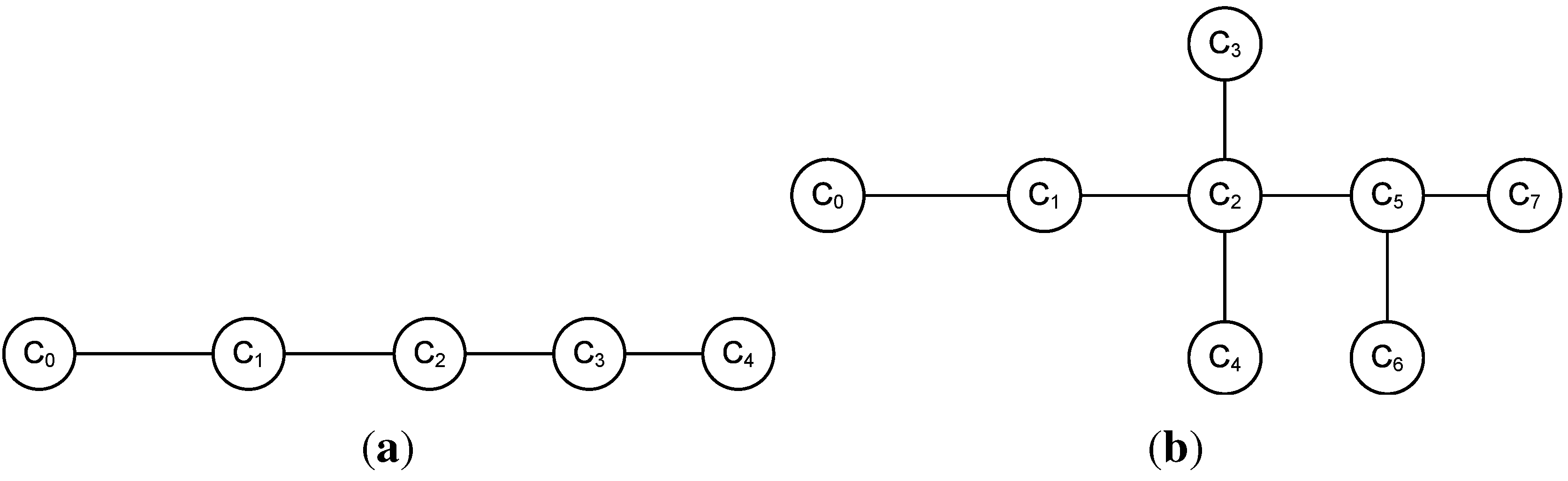
• All the chains of the proposed topology are simple chains, rather than complex chains. A simple chain is defined as a chain where each member node of the chain has, at the most, two neighbouring nodes. On the other hand, a member node may have more than two neighbouring nodes in a complex chain. Figure 3 shows an example of both simple chain and complex chain. Note that in Figure 3 the member node $C_2$ has four neighbouring nodes—$C_1$, $C_3$, $C_4$, and $C_5$.
• In a lower-level chain, the distances between any two successive nodes are called links. Thus, a chain that consists of n number of sensor nodes has $(n-1)$ links. The sum of these $(n-1)$ links is the length of that chain.
• The length of each chain of the proposed topology is similar. As it is assumed that the sensor nodes are deployed randomly in the target field, constructing multiple chains having exactly the same length may not always be possible. However, the proposed logical topology creates chains of similar lengths to avoid uneven energy consumptions by chains of dissimilar lengths.
• For each chain, a member node of the chain is elected as the leader of the chain. These leaders are called lower-level leaders.
• The lower-level leaders construct a higher-level chain. Similarly, a member node of the higher-level chain is elected as the leader of the chain. This leader is called the higher-level leader.

Figure 3. Types of chains: (a) simple chain; (b) complex chain.

Figure 3. Types of chains: (a) simple chain; (b) complex chain.

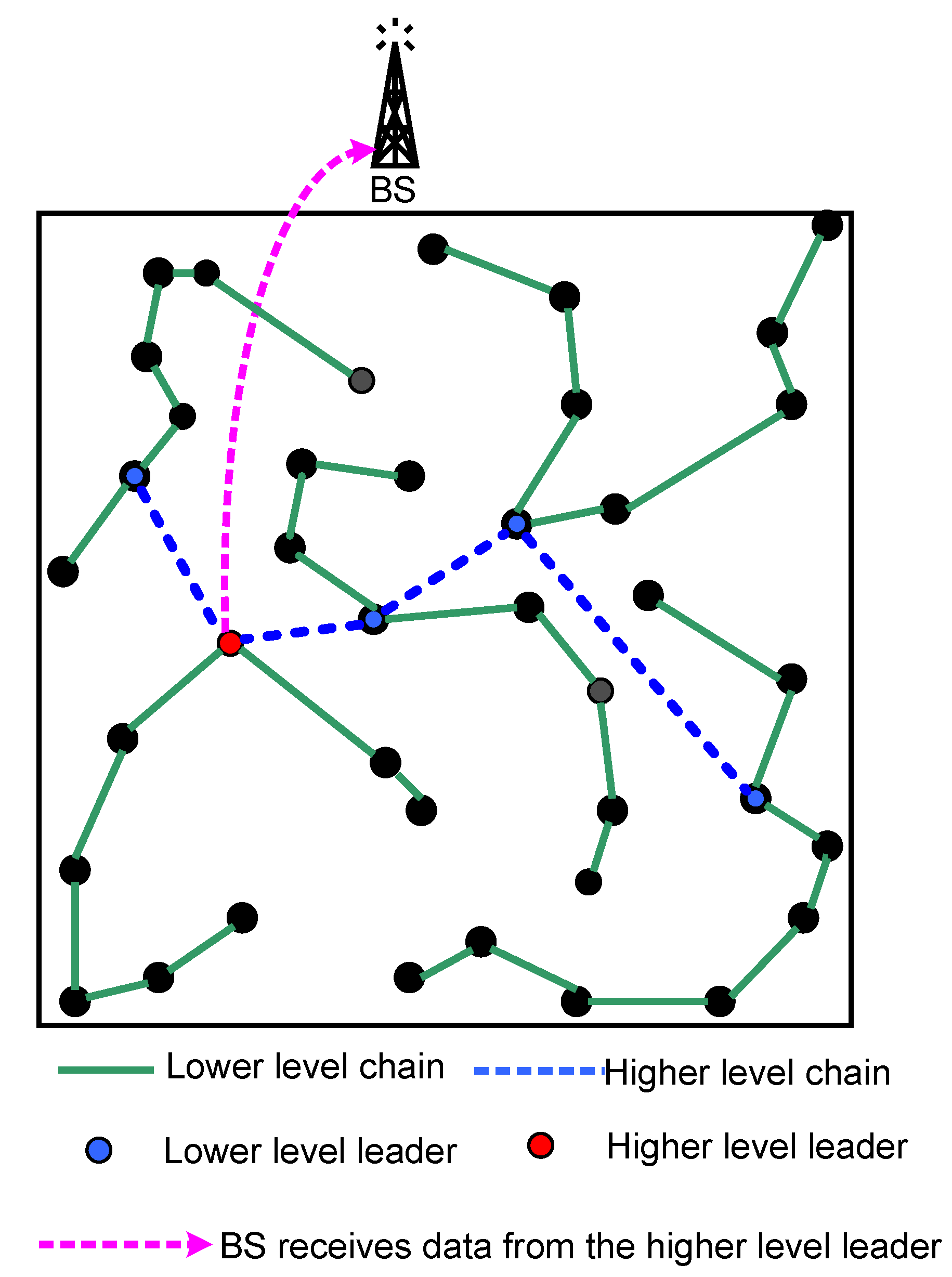
A sample architecture model of the proposed logical topology is depicted in Figure 4. This figure shows the logical topology using two hierarchical layers.

Figure 4. A sample model of the proposed topology.

Figure 4. A sample model of the proposed topology.

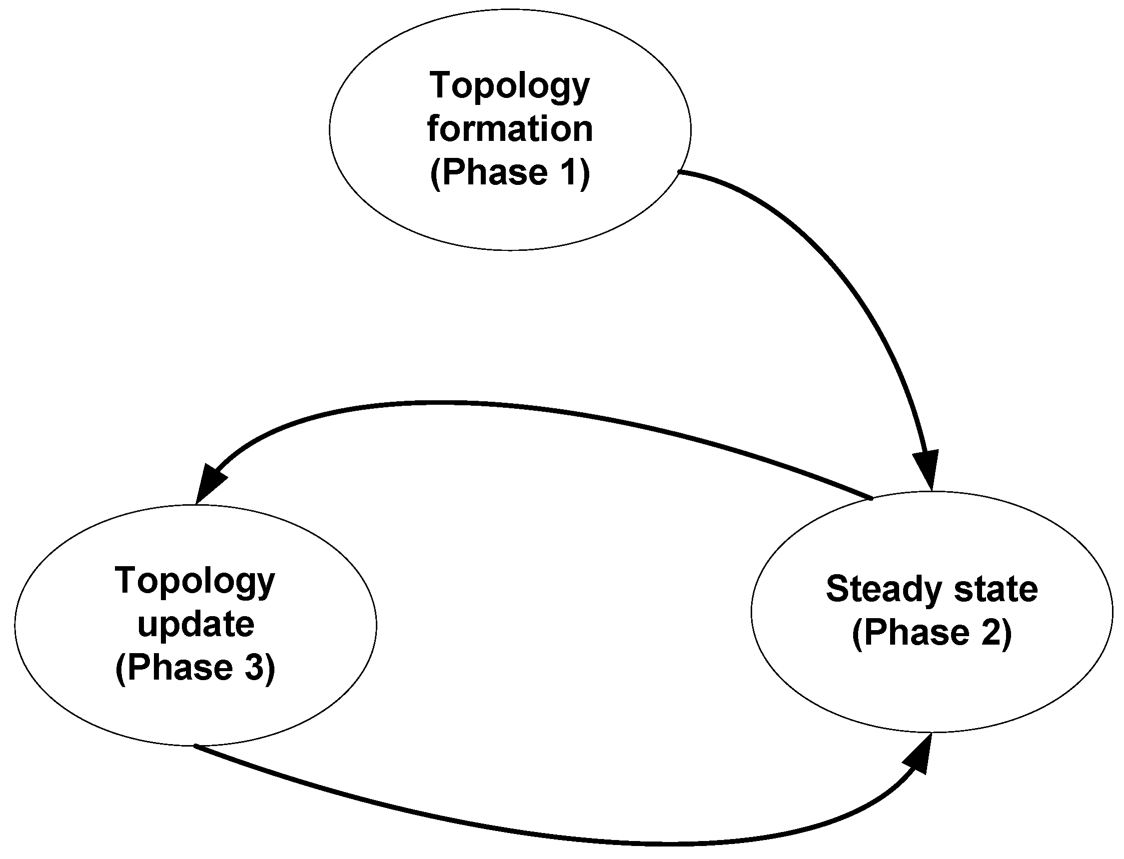
4.2. Different Phases of the Proposed Topology

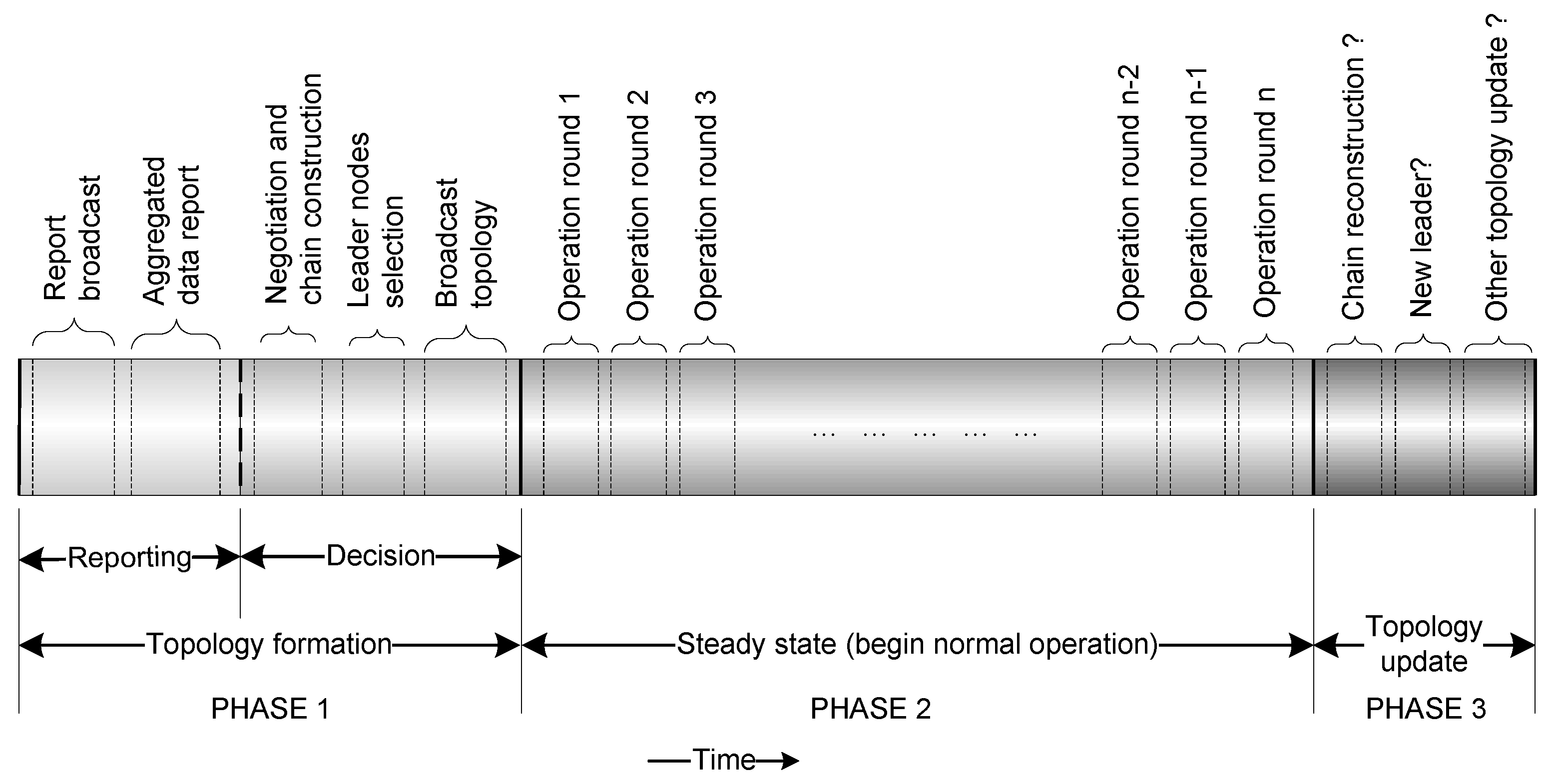
The proposed logical topology can be described using three phases, namely (i) topology formation phase; (ii) steady state phase; and (iii) topology update phase. Figure 5 demonstrates these phases with respect to a timeline. Additionally, Figure 6 demonstrates the transitions among different phases.

Figure 5. Timeline of the proposed topology.

Figure 5. Timeline of the proposed topology.

Figure 6. Transitions of different phases of the proposed topology.

Figure 6. Transitions of different phases of the proposed topology.

At the initial stage of the sensor deployment in the target field, the topology formation phase starts. This phase takes place only once. The steady state phase and the topology update phase then follow. At the beginning of the topology formation phase, no sensor nodes recognise any other sensor node in the target field. Each of the deployed sensor nodes then reports its individual characteristics to all of its neighbouring sensor nodes using broadcasting. A sensor node, receiving broadcasted messages by its neighbouring nodes, calculates the distances between itself and the neighbouring nodes. Additionally, each sensor node aggregates the reports it collects from its neighbouring nodes. After reporting, all the sensor nodes negotiate with their neighbours and construct several chains. When the chain constructions finish, lower-level leaders are elected for each chain. Each lower-level chain then broadcasts the topology, describing the member nodes, successor-predecessor lists, and time division multiple access (TDMA) allocations. At this point, the topology formation phase ends, and the deployed sensors are ready for their normal operation.

At the end of the topology formation phase, the steady state phase begins. In this phase, the sensor nodes start their normal operation. Without the loss of generality, it can be assumed that the sensors are deployed in the target field to collect some data. The steady state consists of several rounds. A round begins whenever the sensor nodes start their sensing. A round finishes when the higher-level leader collects all sensed data via the lower-level leaders, and then sends the data to the BS.

After the end of a fixed number of rounds in the steady state, the topology update phase takes place. The tasks of this phase are to maintain the topology, such as selection of new lower-level leaders, construction of a higher-level chain, selection of a higher-level leader, and reconstruction of chains, if necessary.

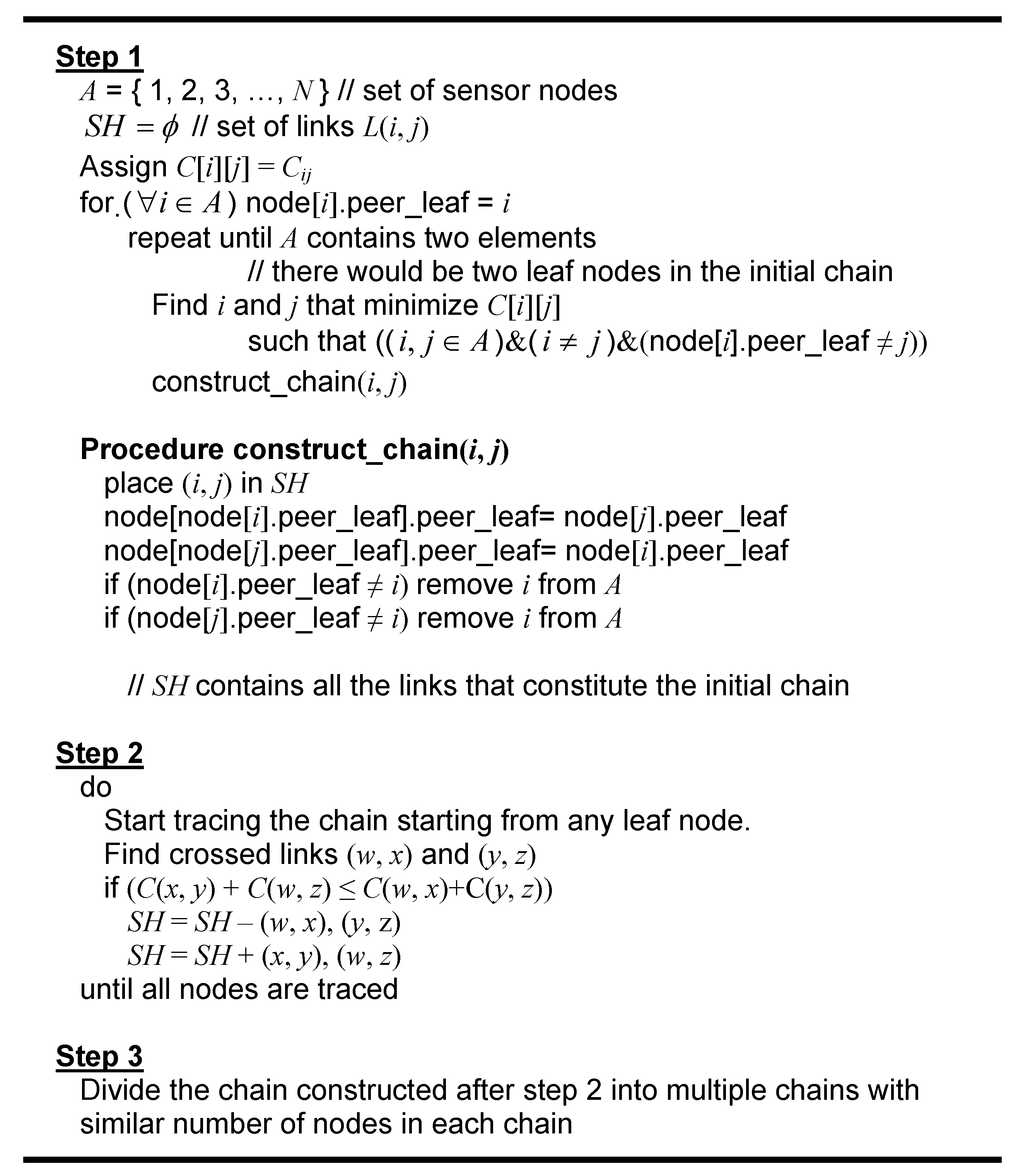
4.3. Chain Construction Algorithm for the Proposed Topology

The proposed chain construction algorithm consists of three steps, namely (i) generating the shortest-path chain; (ii) link exchange; and (iii) pruning. Step one generates an initial single chain, which is derived using the Kruskal minimum spanning tree algorithm. This initial chain may not be optimised, because of the existence of some cross links. At steps two and three, these cross links are removed, and the chain is reconstructed and pruned to multiple chains. The chain construction algorithm is depicted in Figure 7, and detailed descriptions of each step are provided below.

Figure 7. Chain construction algorithm.

Figure 7. Chain construction algorithm.

Step 1. Configuring the initial chain. This step generates an initial chain, which is derived from the Kruskal minimum spanning tree algorithm by giving an additional constraint of a maximum degree of 2. This algorithm selects a link, one by one, through a specified routine. Since links are selected as long as a loop does not occur, several complex chains (see Figure 3(b)) can be generated during the chain generation. When some links are formed, the next link is the shortest link among links that connect those nodes whose degree is under 2. However, the two end nodes are not included in the same sub-chain.

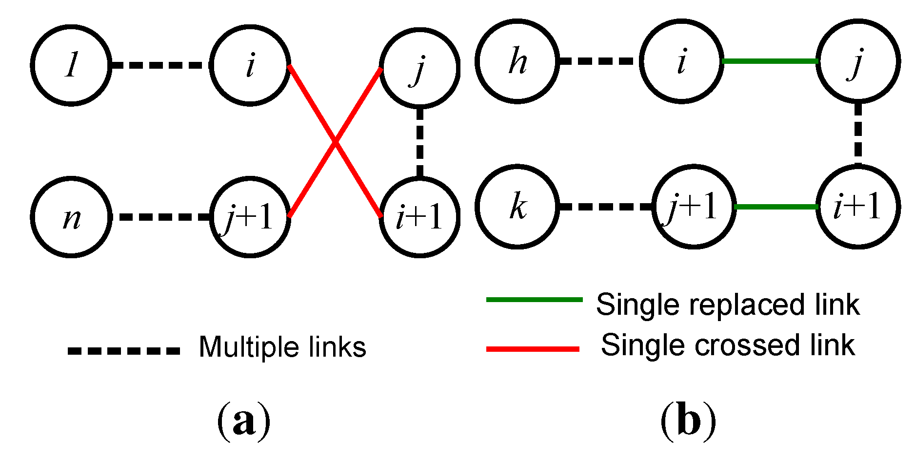
Step 2. Link Exchange. For large number of nodes, there is a high possibility that the initial chain generated after step 1 includes some cross links (see Figure 8). In this step, cross links are removed, and the chain is pruned to multiple chains. The cross link removal process takes place when there are available links whose lengths are shorter than that of the cross links. This process is called link exchange.

In Figure 8, the nodes are numbered from 1 to n. In this figure, dotted lines represent sub-chains that are consisted of several links. The solid lines in this figure represent a single link. When the process of link exchange occurs, the order of sub-chain from $i+1$ to j is reversed. To exchange two links of the chain as from $(i,i+1)$ and $(j,j+1)$ to $(i,j)$ and $(i+1,j+1)$, the following condition should be satisfied: $C(i,i+1)+C(j,j+1)\ge C(i,j)+C(i+1,j+1)$ where $C(i,j)$ denotes the length of the link $(i,j)$.

Figure 8. Link exchange. Crossed links are replaced by new links.

Figure 8. Link exchange. Crossed links are replaced by new links.

Step 3. Pruning. At the end of the link exchange, an optimal chain is generated. To create multiple chains from this optimal chain, each node of this chain is traced, starting from the farthermost end of the chain from the BS. The tracing process takes place from one node to its neighbouring node until the number of nodes traced is equal to $C_N$. Here, $C_N$ is the optimal number of node in a chain. At this point all nodes that have already been traced are pruned from the initial chain. This pruning process continues until all the nodes of the initial chain are traced.

4.4. Selection of Leader Nodes

Given a chain structure, leader scheduling determines which nodes play the role of leaders in operational rounds. The goal is to prolong network lifetime, i.e., to maximise the number of operational rounds. The following discusses the general issues about selecting leader node(s) with respect to power consumption.

Suppose any node in a chain can be elected as a leader, and the leader is responsible to send the aggregated data to the BS. The maximum number of operational rounds that can be achieved before any node exhausts its power is analysed first. Without loss of generality, it can be assumed that nodes in the chain are numbered sequentially as $1,2,\dots ,n$. Let $e_i$ be the energy consumed by the node i in transmitting a data message to the BS. Let ${\rho }_{i,j}=k{E}_{elec}+k{ϵ}_{amp}{\left(d(i,j)\right)}^{\alpha }$ be the energy consumed by the node i, and $e_r=k{E}_{elec}$ be the energy consumed by the node j when the node i transmits a k-bit message to the node j. When a node i is selected to be the leader, every node numbered $j<i$ (if any) expends ${\rho }_{j,j+1}$ energy in sending data to the node $j+1$, at which energy $e_r$ is consumed to receive the data. Likewise, every node numbered $k>i$ (if any) expends ${\rho }_{k,k-1}$ to send data to the node $k-1$, where energy $e_r$ is expended in receiving the data. The leader transmits the collected data to the BS, consuming energy $e_i$. Suppose that, every node i is scheduled to be the leader $x_i$ times. Table 1 shows the energy expense of every sensor node in this case.

Table 1. Energy consumption by different nodes while acting as a leader.

Node ID	Energy spent to send message to the BS	Energy spent to neighbours	Energy spent to receive neighbour’s message
1	$e_1{x}_1$	${\rho }_{1,2}{\sum }_{j=2}^n{x}_j$	$e_r{x}_1$
$i\in \{2,3,\dots ,n-1\}$	$e_i{x}_i$	${\rho }_{i,i-1}{\sum }_{j=1}^{i-1}{x}_j+{\rho }_{i,i+1}{\sum }_{j=i+1}^n{x}_j$	$e_r\left({\sum }_{j=1}^{i-1}{x}_j+2x_i+{\sum }_{j=i+1}^n{x}_j\right)$
N	$e_n{x}_n$	${\rho }_{n,n-1}{\sum }_{j=1}^{n-1}{x}_j$	$e_r{x}_n$

$x_i$ : the number of times node i is selected to be the leader; $e_i$ : the amount of energy consumed in transmitting message from node i to BS; ${\rho }_{i,j}$: the energy consumed by i in transmitting a message to j; $e_r$ : the energy consumed by any node in receiving a message.

Table 1. Energy consumption by different nodes while acting as a leader.

Node ID	Energy spent to send message to the BS	Energy spent to neighbours	Energy spent to receive neighbour’s message
1	$e_1{x}_1$	${\rho }_{1,2}{\sum }_{j=2}^n{x}_j$	$e_r{x}_1$
$i\in \{2,3,\dots ,n-1\}$	$e_i{x}_i$	${\rho }_{i,i-1}{\sum }_{j=1}^{i-1}{x}_j+{\rho }_{i,i+1}{\sum }_{j=i+1}^n{x}_j$	$e_r\left({\sum }_{j=1}^{i-1}{x}_j+2x_i+{\sum }_{j=i+1}^n{x}_j\right)$
N	$e_n{x}_n$	${\rho }_{n,n-1}{\sum }_{j=1}^{n-1}{x}_j$	$e_r{x}_n$

$x_i$ : the number of times node i is selected to be the leader; $e_i$ : the amount of energy consumed in transmitting message from node i to BS; ${\rho }_{i,j}$: the energy consumed by i in transmitting a message to j; $e_r$ : the energy consumed by any node in receiving a message.

The optimal leader scheduling problem is to find positive integer values of $x_i$’s to maximise ${\sum }_i{x}_i$ subject to the following constraints:

$$\begin{array}{c}{E}_1\ge (e_1+e_r)x_1+{\rho }_{1,2}{x}_2+{\rho }_{1,2}{x}_3+\dots +{\rho }_{1,2}{x}_n\hfill \\ ⋮\hfill \\ E_i\ge ({\rho }_{i,i-1}+e_r)x_1+\dots +({\rho }_{i,i-1}+e_r)x_{i-1}+(e_i+2e_r)x_i+({\rho }_{i,i+1}+e_r)x_{i+1}+\dots +({\rho }_{i,i+1}+e_r)x_n\hfill \\ ⋮\hfill \\ E_n\ge {\rho }_{n,n-1}{x}_1+{\rho }_{n,n-1}{x}_2+\dots +(e_n+e_r)x_n\hfill \end{array}$$

where $E_i$ denotes the amount of energy that node i initially has.

These constraints can be formulated as

$$A\left(\begin{array}{c}{x}_1\\ x_2\\ x_3\\ ⋮\\ x_n\end{array}\right)\le \left(\begin{array}{c}{E}_1\\ E_2\\ E_3\\ ⋮\\ E_n\end{array}\right)$$

where

$$A=\left(\begin{array}{cccc}{e}_1+e_r& {\rho }_{1,2}& \cdots & {\rho }_{1,2}\\ {\rho }_{2,1}+e_r& e_2+2e_r& \cdots & {\rho }_{2,3}+e_r\\ {\rho }_{3,2}+e_r& {\rho }_{3,2}+e_r& \cdots & {\rho }_{3,4}+e_r\\ ⋮& ⋮& \cdots & ⋮\\ {\rho }_{n,n-1}& {\rho }_{n,n-1}& \cdots & e_n+e_r\end{array}\right)$$

Thus, the problem becomes a linear programming problem. Round robin leader scheduling equalises the values of $x_i$’s, which is generally far from optimal. The authors of PEGASIS also proposed an improvement on round robin scheduling [40]. This approach sets up a threshold of distance, and nodes are not allowed to be leaders if the distance to their neighbours along the chain is beyond the threshold.

From the above discussion, the ability to achieve optimal results in leader selection is a computationally rigorous task. Thus, instead of finding an optimal solution, the proposed topology uses a simple rule called Maximum Residual Energy First (MREF) for leader selection. This simple algorithm gives near optimal results for a lower number of nodes. As in the proposed topology, there are only a few lower-level leaders, making this algorithm perfectly suitable for selecting a higher-level leader. As the name suggests, MREF selects the node that has the maximum residual energy to be the leader for network operations. Residual energy information can be piggybacked with data messages as a part of the aggregated data. If every lower-level leader attaches its own energy level to data message and lets the BS find the maximum value, it will incur an additional $O\left(n\right)$ overhead on every message. A better approach is to let every lower-level leader compare its energy level with the energy level attached to the incoming data message (if any) and send only the large one. The message overhead in this process is only $O\left(1\right)$.

For the lower-level leaders, the same selection procedures can be followed. However, since the communications of the lower-level leaders are not as energy intensive as for higher-level leader, it is proposed not to change lower-level leaders as frequently as higher-level leader. The benefits of using a slightly longer duration for selecting lower-level leaders include: (i) less communication overhead; (ii) reduced required time for leader selection at every round; and (iii) maximum utilization of the higher-level chain.

4.5. Design Issues of the Proposed Logical Topology

Design issues that need to be discussed in relation to the proposed logical topology include the number of chains in the system, the number of nodes in a chain, and the time when the leaders should be changed or the chains should be reconstructed/updated. Other issues regarding network management include the arrival of a new node, or dead/aberrant nodes. These issues are discussed below.

4.5.1. Total Number of Chains in the System and Optimal Number of Nodes in a Chain

The system can determine, a priori, the optimal number of chains (lower-level) for a particular system. This depends on several parameters, such as the positions of the sensor nodes, and the relative costs of computation versus communication. The proposed topology was simulated for a data collection application using a network where a number of sensor nodes were randomly deployed. The value of the radio parameters of the transmitter and the receiver that were used in the simulation are $E_{tx-elec}=E_{Rx-elec}=E_{elec}=50$ nJ/bit. The transmit amplifier was assumed to be 100 pJ/bit/$m^2$. A computation cost of 5 nJ/bit/message to fuse 2000-bit messages was further assumed. In the experiment, the number of chains in the system was varied gradually in order to observe its impact on energy consumption, and delay. The experiment was repeated varying the total number of sensor nodes (100, 200, 300, 400, and 500). 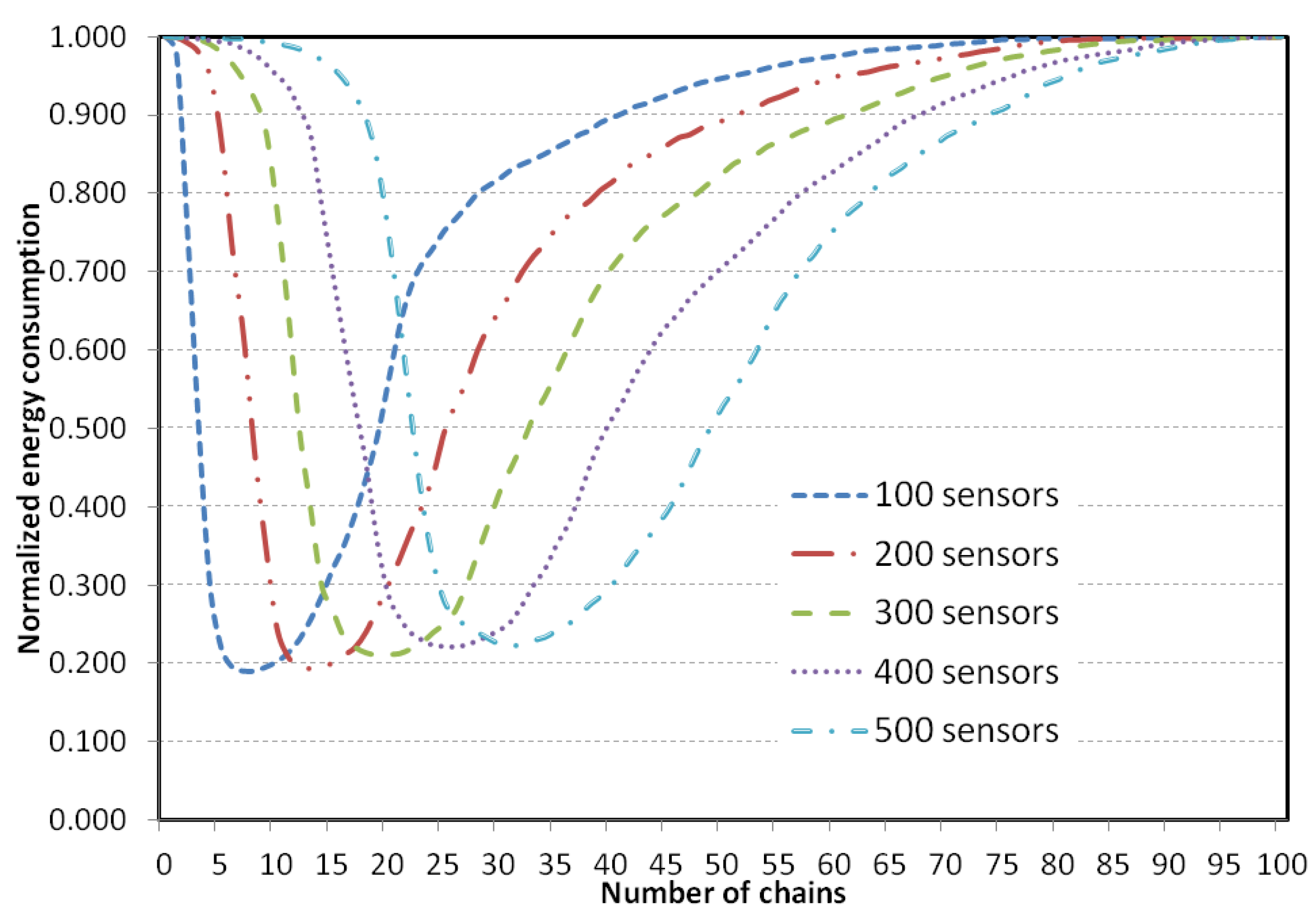Figure 9 shows how the energy dissipation in the system varies with the number of chains in the system. Note that a zero chain means that no lower-level chain, and thus no higher-level chain, is constructed. In this situation, each sensor node directly transmits its sensed data to the BS. Also note that, 1 chain means there would be no higher-level chain, and 100 chains means there is actually no lower-level chain (because each chain has only one member) and only a single higher-level chain. Therefore, both 1 chain and 100 chains refer to the same system as PEGASIS. Figure 9 shows that for a 100-node network, energy dissipation is minimum when 5 to 10 chains are created. For a 200-node network, energy consumptions is minimum when 10–20 chains are created with 200 nodes in the network. For a network of 300 nodes in it, the energy consumption is minimum when 16 to 25 chains are created. For a 400-node network it is from 22 to 32, and finally for a 500-node network, 27–38 chains consume the least energy. However, a large number of chains would cause more overhead. Thus, for the proposed topology, the number of chain is maintained at 6%–8% of the sensor nodes. Therefore, for a target field of 200 sensor nodes deployed, 12 to 16 chains would be constructed. This calculation almost matches with the calculation provided in [41].

Figure 9. Normalised total system energy dissipated versus number chains constructed.

Figure 9. Normalised total system energy dissipated versus number chains constructed.

The optimal number of nodes in a chain, denoted as $C_N$, is the number of nodes that should be included in each chain during the chain construction phase. It can be argued that, if the number of nodes in a chain is fewer than $C_N$, both the required time and energy dissipation increase in the network. On the other hand, if the number of nodes is more than $C_N$, energy dissipation may decrease slightly, but the time requirement increases. Additionally, for the sake of even energy dissipation distribution, the lengths of the chains should be similar. Thus, in the proposed scheme, a similar number of sensor nodes are included for each chain. Since it is assumed that sensors are deployed randomly in the target field, creating chains of exactly the same number of sensor nodes may not be possible. However, the proposed scheme maintains a similar number of nodes in each chain. Thus for a target field of 100 nodes, the number of chains is between 6 to 8, and each of the chain contains around 17 to 12 sensor nodes respectively ($C_N$ = 12 to 17).

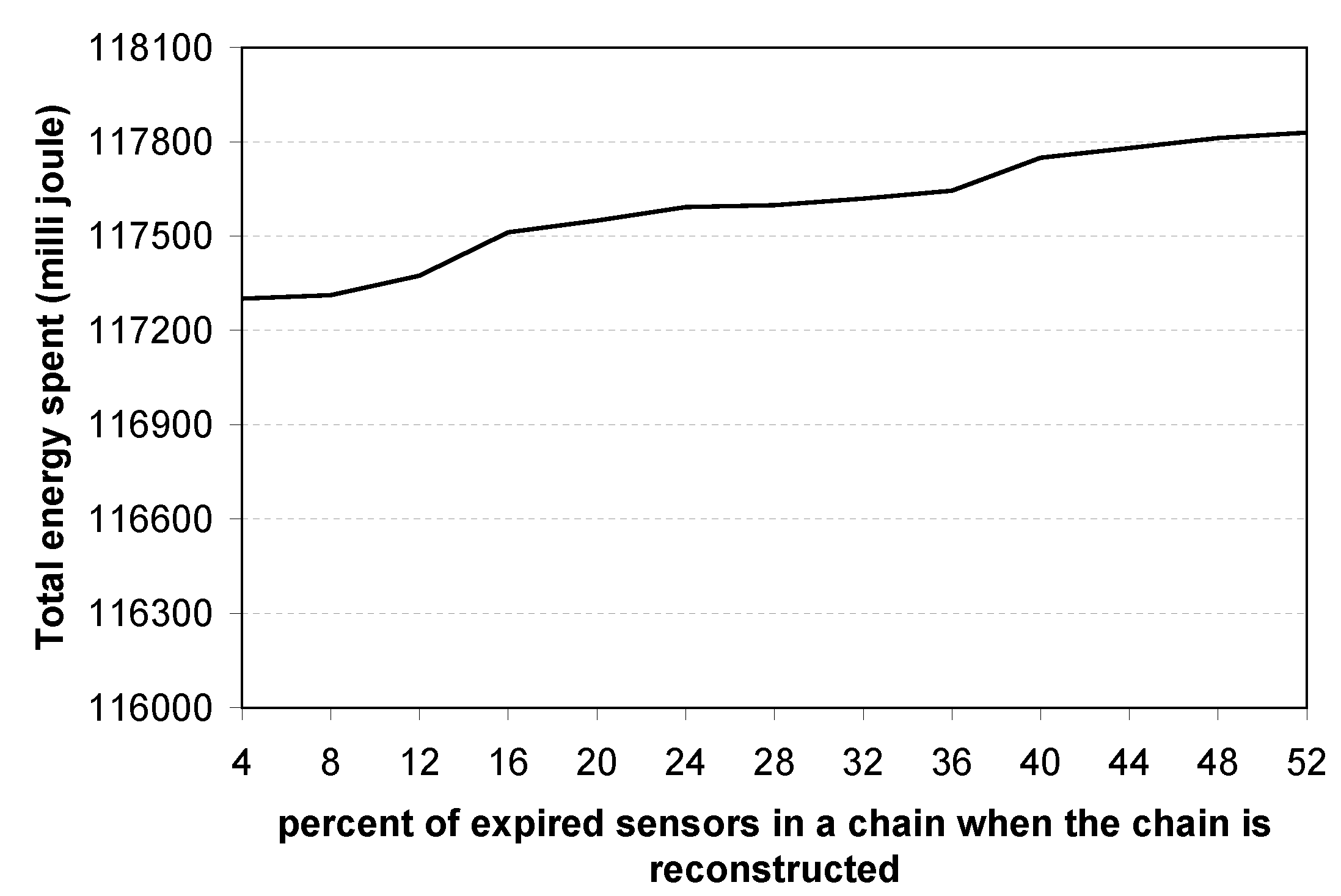
4.5.2. Chain Reconstruction

It is important to reconstruct the chains whenever a significant number of sensor nodes in a chain expire. Otherwise, one chain may contain a higher number of sensor nodes, while others may contain a lower number of sensors. This affects the performance of the topology due to uneven energy dissipation by the chains. 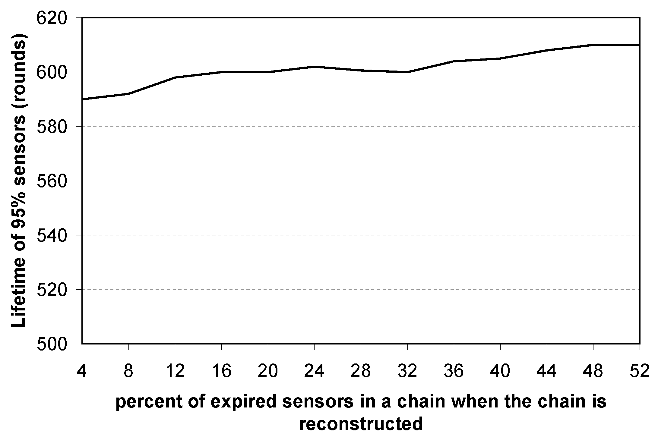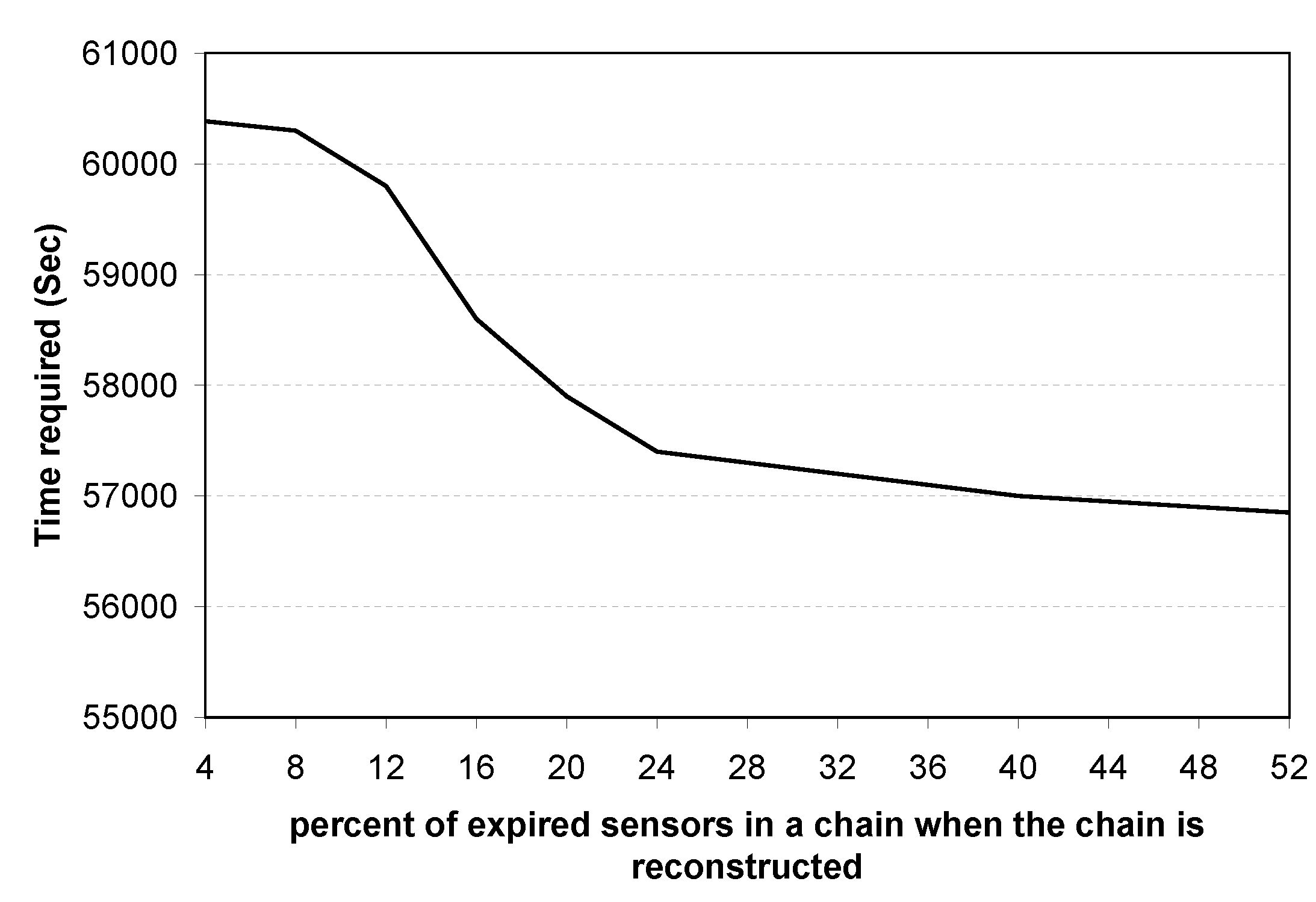It is vital to maintain uniformity in the number of sensor nodes in all chains as only one sensor node (i.e., the higher-level chain leader) is responsible for sending the aggregated data to the BS, and it has to wait for aggregated data from different lower-level leaders. Thus, the uniformity of number of sensors in chains affects network lifetime. If a chain consists of a lower number of sensors, the probability of a sensor in that chain being selected as a local leader will be higher. Thus, a chain of short length is likely to lose sensors more often. It is obvious that if chains are reconstructed frequently, such as whenever only 4%–5% sensors of the chain die, it causes extra overhead. On the other hand, if the chain is reconstructed whenever 40%–50% sensors of the chain die, the uniformity among the chains is destroyed. To answer the question of when a chain should be reconstructed, simulation experiments were performed. To find the optimal value, chains were reconstructed varying the percentage of sensors’ death in the chains, and its effects on total energy spent, lifetime of the network, and time required to complete 100 rounds were observed. Simulation results are presented in Figure 10, Figure 11 and Figure 12. Figure 10 shows that although the energy consumption increases when chains are reconstructed less frequently, the amount of energy difference is not extreme. Figure 11 shows that the lifetime of 95% of the deployed sensor nodes remains almost steady regardless of the percentage of expired sensors when a chain is reconstructed, with a small peak when approximately 20% of the deployed sensors have expired. Figure 12 shows that time requirements decrease when chains are reconstructed less frequently. Time requirement falls sharply when 4%–20% sensors die and then decreases slowly afterwards. Thus, it is concluded that it is best to reconstruct chains when approximately 20% of the sensors within a chain expire.

To track how many sensor nodes are expired in a chain, the following method can be used. When data are fused in every sensor of a chain, each sensor adds its tag to the data packet. For example, let node $n_1$ send data to $n_2$, and $n_2$ fuse $n_1$’s data and send it to $n_3$. However, if $n_2$ is dead, $n_1$ sends data directly to $n_3$, and thus the node $n_3$ knows that $n_2$ is dead. In this way every lower-level leader can determine how many of its members are dead. In a similar fashion, when the higher-level leader collects data from all lower-level leaders, it can determine how many sensors in the network are dead. Subsequently, the higher-level leader sends instructions to all sensor nodes.

Figure 10. Total energy spent vs. percent of expired sensor nodes in a chain when the chain is reconstructed.

Figure 10. Total energy spent vs. percent of expired sensor nodes in a chain when the chain is reconstructed.

Figure 11. Network lifetime vs. percent of expired sensor nodes in a chain when the chain is reconstructed.

Figure 11. Network lifetime vs. percent of expired sensor nodes in a chain when the chain is reconstructed.

Figure 12. Time required vs. percent of expired sensor nodes in a chain when the chain is reconstructed.

Figure 12. Time required vs. percent of expired sensor nodes in a chain when the chain is reconstructed.

4.5.3. Changing Lower-Level Leaders

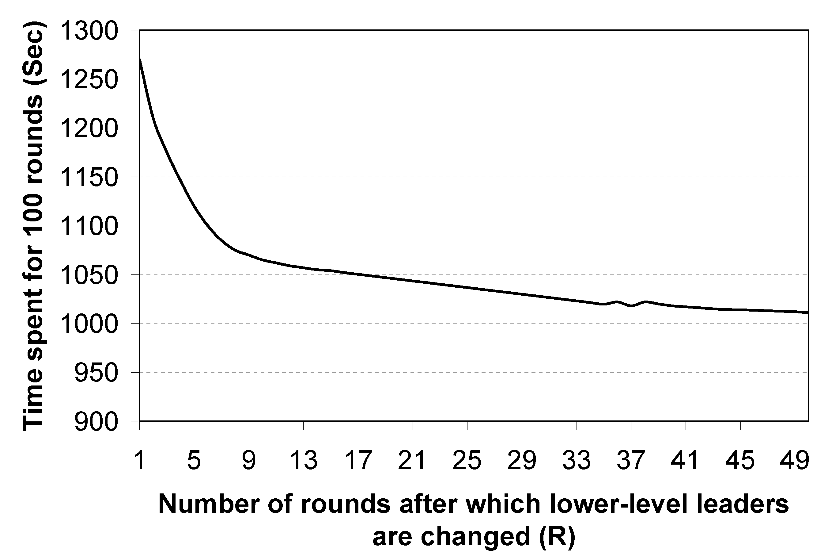
The lower-level leaders should be changed periodically to distribute the energy load. PEGASIS suggests changing the leader node in each round. However, for the proposed topology, if the lower-level leaders are changed at every round, it causes extra energy expenditure for negotiations to select leaders, as well as causing delay. In addition, the higher-level chain can be fully utilised if the lower-level leaders are changed after a number of rounds. Conversely, if the lower-level leaders are not swapped with other member nodes for a long time, they will quickly be drained of energy due to excessively long transmissions. Therefore, in the proposed logical topology, lower-level leaders are changed after R rounds, where the value R depends on the following criteria: (i) total energy dissipation in the network; (ii) maximum number of round before the first sensor node dies; and (iii) the delay introduced in the network for different number of rounds.

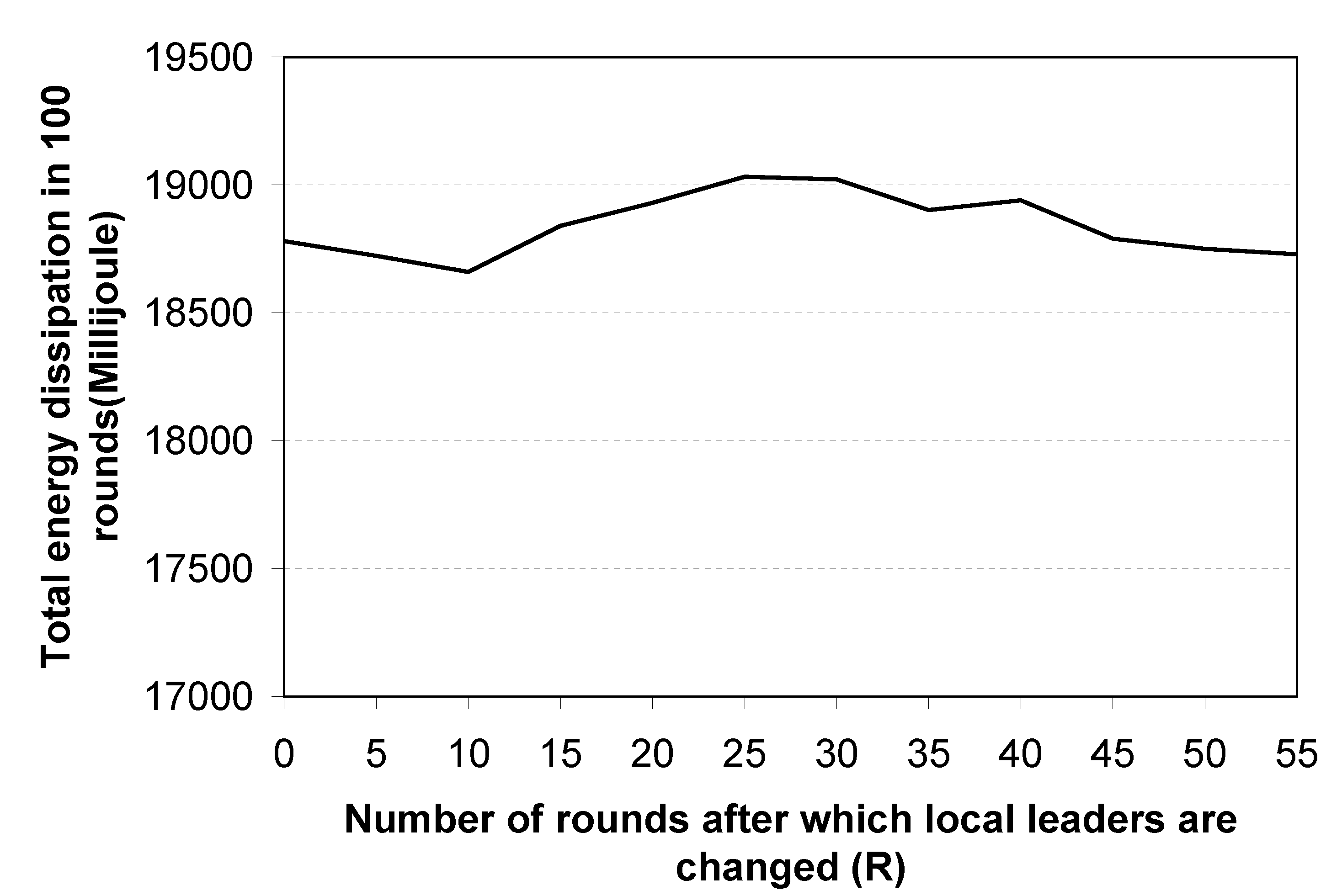
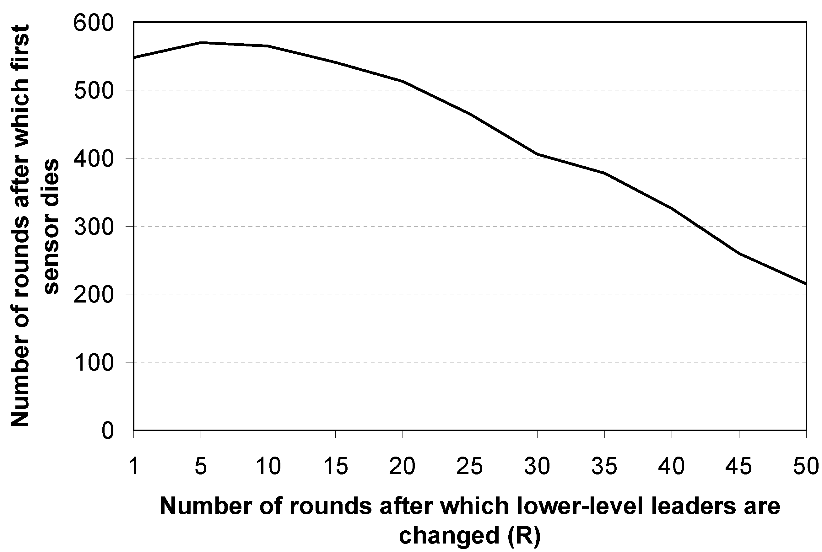
Figure 13, Figure 14 and Figure 15 show the simulation results, which are used to determine when the lower-level leaders should be changed. Figure 13 shows the relationship between R and the total energy spent in the network. The figure shows that there is no correlation between total energy consumption and R. In contrast, Figure 14 shows that as the value of R increases, the network lifetime decreases. This is because, when the same sensor nodes are working as leaders for long periods, they deplete energy quickly compared with other sensor nodes. Figure 15 shows that the time delay decreases as the value of R increases. In conclusion, from the experimental results, shown in Figure 13, Figure 14 and Figure 15, it is proposed that the lower-level leaders should be changed after $C_N/2$ rounds.

Figure 13. Leader selection time vs. total energy dissipation.

Figure 13. Leader selection time vs. total energy dissipation.

Figure 14. Leader selection time vs. network lifetime.

Figure 14. Leader selection time vs. network lifetime.

Figure 15. Leader selection time vs. time required.

Figure 15. Leader selection time vs. time required.

4.5.4. Inserting Additional Nodes into the Network

Additional nodes may be inserted into the network at any time. Before a node is inserted, the BS records and stores its unique ID and will insert the node into a nearby chain with the least number of nodes. This helps to minimise the chance of a chain monopolising a certain bandwidth if it contains a greater number of nodes than other chains that are communicating. The node will then organise itself within its chain.

4.5.5. Identifying and Isolating Aberrant Nodes

Sensor nodes that do not function as specified must be identified and isolated in order to continue the desired operation of the sensor network. An aberrant node may be the result of an attack or may act maliciously due to unexpected network behaviour. According to [42], an aberrant node is one that is not functioning as specified, and may cease to function as expected for the following reasons:

• it has exhausted its power source or is damaged by an attacker,
• it is dependent upon an intermediate node and is being deliberately blocked because the intermediate node has been compromised,
• an intermediate node has been compromised and is corrupting the communication by modifying data before forwarding it, or,
• a node has been compromised and communicates fictitious information to the BS.

Therefore, the WSN should be maintained by identifying an aberrant node quickly and isolating it from the sensor network. The protocol named SecCOSEN [28] can be used for authentication purposes. This protocol perfectly suits the logical topology, as it was designed for a multiple chain oriented logical topology. Using this protocol, a node can authenticate the node from which it receives data/messages. If a node is not able to authenticate another node in the chain, the former node reports the incident to the chain leader. In addition, a node also maintains a timer for identifying any dead node with the help of timeouts and reports the incident to the leader node.

4.5.6. Number of Layers

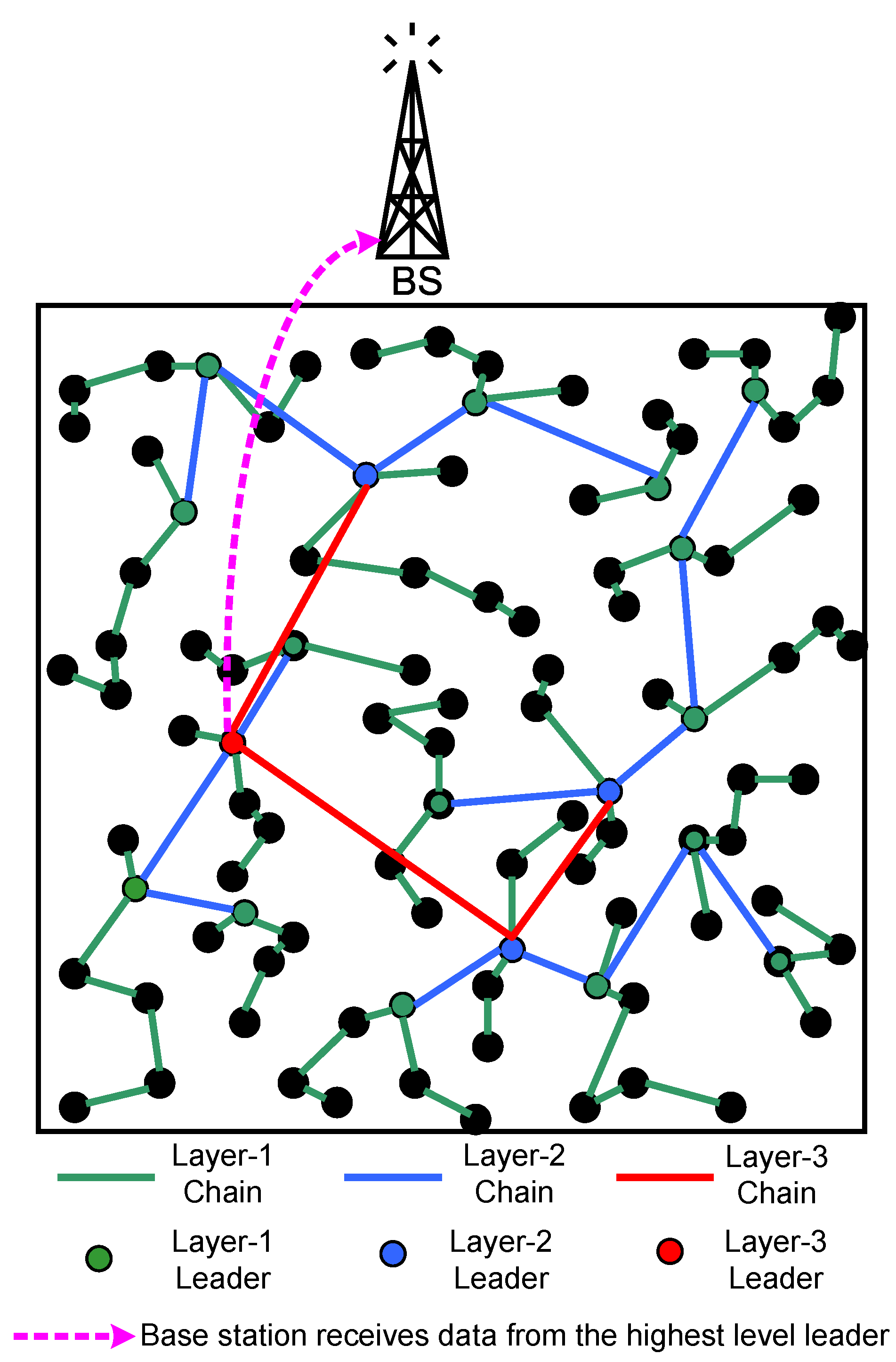
Although we describe the proposed multiple chain oriented logical topology using a two-layer model, the number of layers can be extended based on the number of sensor nodes in the target field. For example, Figure 16 depicts a model of multiple chain oriented logical topology with three hierarchical layers. In this figure, the black nodes are the member nodes of layer-1 green-coloured chains. In each layer-1 chain, a node is elected as a leader and marked in green. All green-coloured layer-1 leaders construct several layer-2 blue coloured chains. Similarly, in each layer-2 chain, a node is elected as a leader marked in blue. All the blue-coloured layer-2 leaders further construct a layer-3 chain, and one of its members is elected as a leader. This leader is the highest level leader, and is marked in red. A black node sends the data to its leader (green) via the green chain, a green node sends the accumulated data to its leader (blue) via the blue chain, and finally, a blue node sends its accumulated data to its leader (red). The highest level leader (red) then sends the data to the BS.

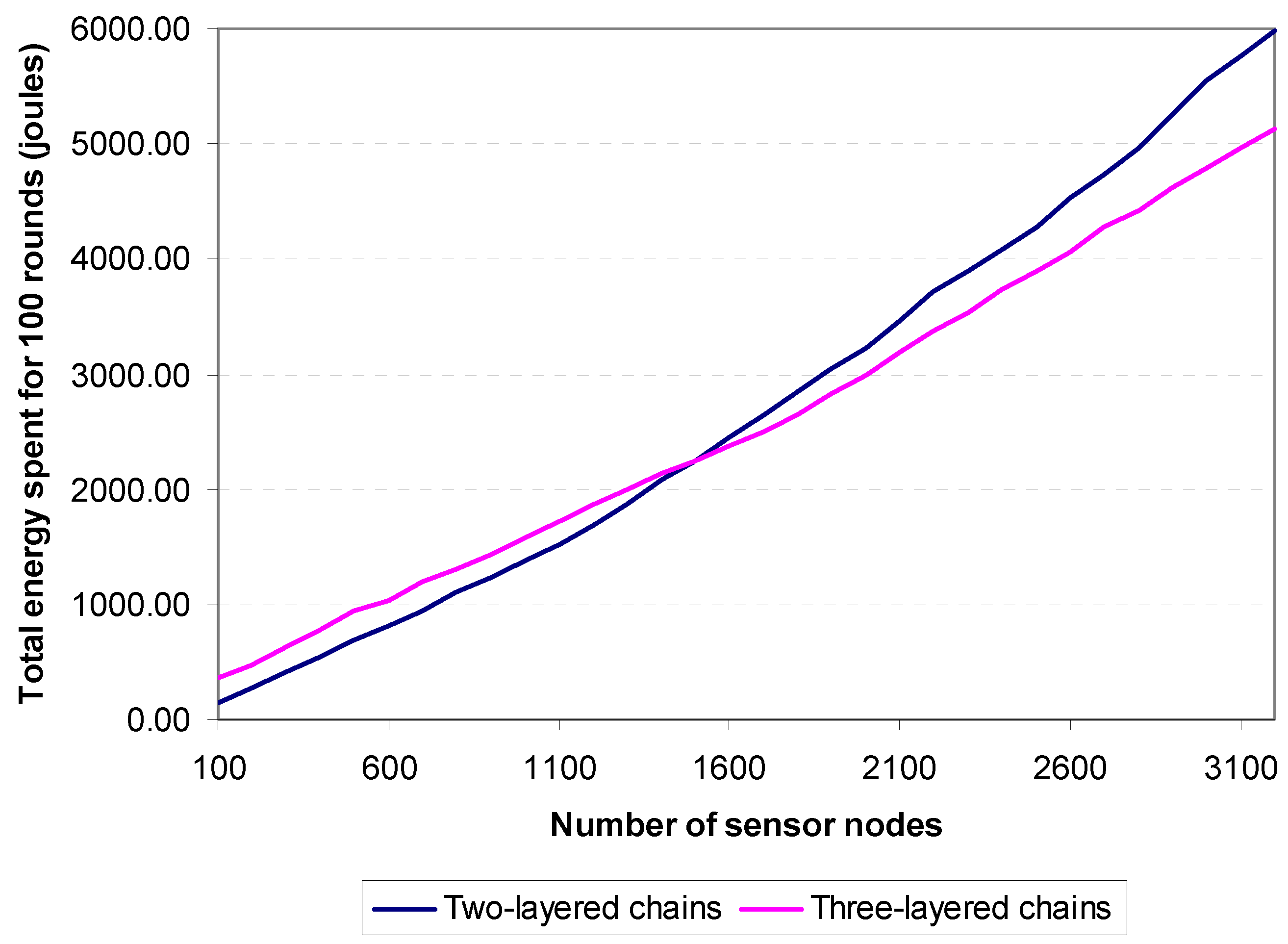
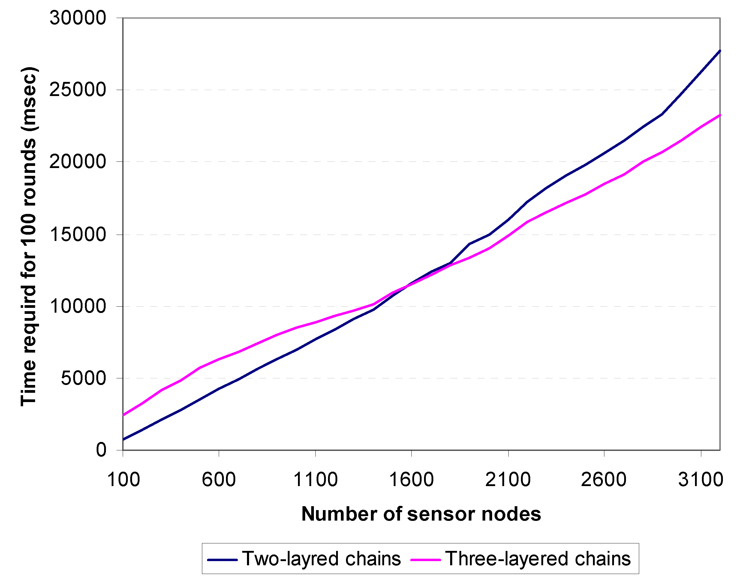
For a large scaled sensor network, a two-layer model may not be suitable, because layer-2 chain in that can be excessively long. On the other hand, for a WSN with several hundred nodes, a three-layer design would be wasting more energy and time, because sensor data would have to be propagated through various hierarchical chains. To find the threshold point, we run a simulation varying the number of sensors from hundred nodes to more than three thousand nodes and measured total energy spent by the system and amount of time required. Figure 17 shows the simulation results and comparison between 2-layered and 3-layered chains with respect to the time required for 100 rounds. The figure demonstrates that 2-layered chains take less time to reach 100 rounds than 3-layered chains until the number of sensors is greater than 1600, when the reverse becomes true. The same situation arises for total energy consumption depicted in Figure 18. The 2-layered architecture saves more energy than the 3-layered architecture up until the number of sensor nodes exceeds 1500, when the reverse becomes true. Thus, it is concluded that, if the number of sensor nodes in the target field is less than 1500, two-layered architecture is used, while if the number of sensor nodes is equal to or greater than 1500, three-layered architecture is more suitable.

Figure 16. Three-layered hierarchical multiple chain oriented topology.

Figure 16. Three-layered hierarchical multiple chain oriented topology.

Figure 17. Timing differences between two-layered and three-layered chains.

Figure 17. Timing differences between two-layered and three-layered chains.

Figure 18. Energy consumption differences between two-layered and three-layered chains.

Figure 18. Energy consumption differences between two-layered and three-layered chains.

4.6. Communication Abstraction of the Proposed Topology

This section describes the communication abstraction for the proposed multiple chain oriented logical topology. Communication is fundamental to any logical topology of WSNs. The power of a WSN comes not from the capabilities of the individual devices, but from the collective capabilities achievable through wireless communication.

Addressing the intricacies of wireless communication can be a difficult and error-prone task. This is especially true of WSN applications, where the number of participating devices can be large, the communication patterns can be complex, and the network links are ad-hoc and unreliable. However, the proposed topology restricts the communications of a sensor node to only its successive nodes in its chain. Thus, the burdens of multicasting and broadcasting are removed from the sensor nodes. The communication abstraction of the proposed topology can be divided into two parts, namely (i) communications within a chain; and (ii) communications between chains.

4.6.1. Communications within a Chain

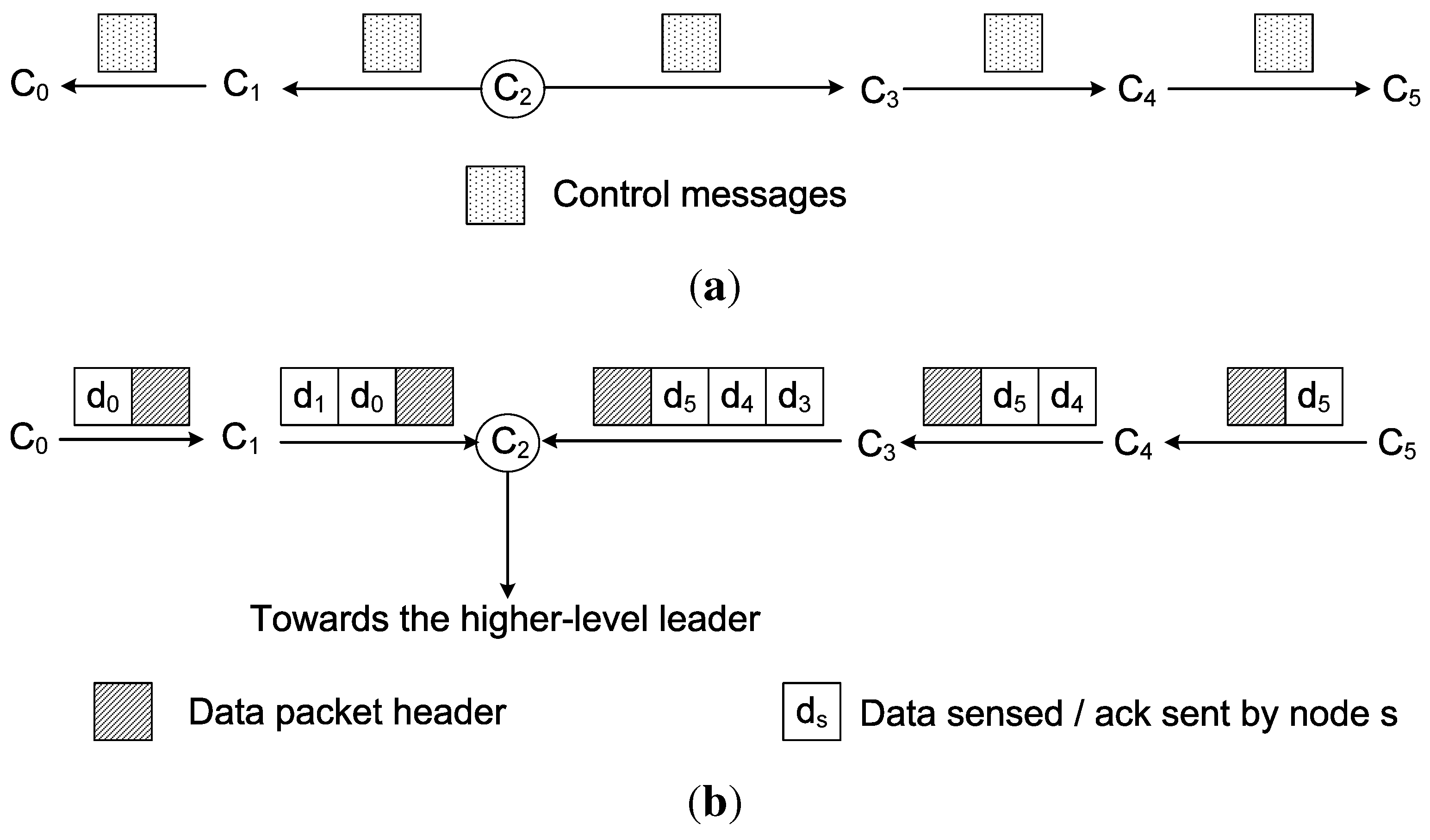
Within a chain, sensor nodes communicate with each other to disseminate control information and sensed data. Communications among the sensor nodes are restricted to only the successive sensor nodes. Figure 19 shows the communication pattern inside a chain. In this figure, six sensor nodes ($C_0$ to $C_5$) construct a chain. $C_2$ is the lower-level leader of the chain. The lower-level leaders disseminate information and control messages to all the member nodes of their chains. These information and control messages are propagated hop-by-hop from one sensor node to its successive neighbouring node. For example, Figure 19(a) shows that the leader node $C_2$ sends the control information to the nodes $C_1$ and $C_3$. After copying the control message, the node $C_1$ sends the control message to the node $C_0$ and $C_3$ sends the message to $C_4$, which then sends it to $C_5$. As the nodes $C_0$ and $C_5$ are the end nodes of the chain, they refrain from sending the control message any further.

Figure 19. Communications in a chain. (a) Control message dissemination; (b) Sending data towards the lower-level leader.

Figure 19. Communications in a chain. (a) Control message dissemination; (b) Sending data towards the lower-level leader.

For sending the sensed data, each sensor node sends data to its successive node towards the leader of the chain. For example, in Figure 19(b), the node $C_0$ sends its sensed data to the node $C_1$, while the node $C_1$ merges its own data with $C_0$’s data, and sends them to the leader node $C_2$. Similarly, the node $C_5$ sends its data to the node $C_4$, and $C_4$ then sends $C_5$’s data and its own data to the node $C_3$. The node $C_3$ accumulates this data with its own data, and sends them all to the leader node $C_2$.

4.6.2. Communication between Chains

Different lower-level chains communicate with each other using the higher-level chain. The lower-level leaders accumulate data sent by the member nodes of the chains, and transfer them to the higher-level leader. The higher-level leader then sends the data to the BS.

If the BS or the higher-level leader wants to send some information or control messages to the chain members, the communication path remains the same, except the direction is opposite. In this case, the communication pattern is similar to hub-and-spoke topology. Figure 20 shows a situation where the BS sends control messages to the member nodes of a chain.

5. Network Management Architecture of the Proposed Topology

This section presents the network management architecture and processes for the proposed logical topology. Network management is the process of managing, monitoring, and controlling the behaviour of a network. The management approach of WSNs differs from the traditional wired networks and mobile ad-hoc wireless networks due to the unique characteristics and restrictions of WSNs.

Figure 20. Communication from the BS to the member nodes of a chain.

Figure 20. Communication from the BS to the member nodes of a chain.

WSN management systems can be classified according to their network architecture: centralised, distributed, or hierarchical. In centralised management systems, the BS acts as the manager station that collects information from all nodes and controls the entire network. However, this approach has some problems. First, it incurs a high message overhead (bandwidth and energy) from data polling, which limits the scalability of WSNs. Second, the central server is a single point of data traffic concentration and potential failure. Lastly, if a network is partitioned, sensor nodes that are unable to reach the central server are left without any management functionality.

Distributed management systems employ multiple manager stations. Each manager controls a sub-network and may communicate directly with other manager stations in a cooperative fashion in order to perform management functions. However, this approach is complex and difficult to manage. Furthermore, distributed management algorithms may be computationally too expensive for resource-constrained sensor network nodes.

Hierarchical network management is a hybrid between the centralised and distributed approach. Intermediate managers are used to distribute management functions, but do not communicate with each other directly. Each manager is responsible for managing the nodes in its sub-network. It passes information from its sub-network to its higher-level manager, and also disseminates management functions received from the higher-level manager to its sub-network. This architecture integrates the benefit of both the centralised and distributed management architecture and is more suitable for WSNs. Consequently, hierarchical network management was chosen for the proposed logical topology.

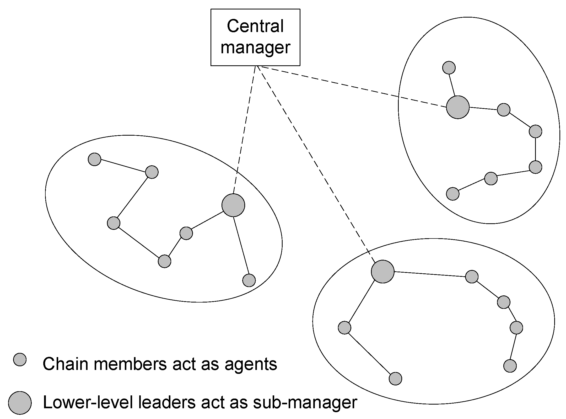
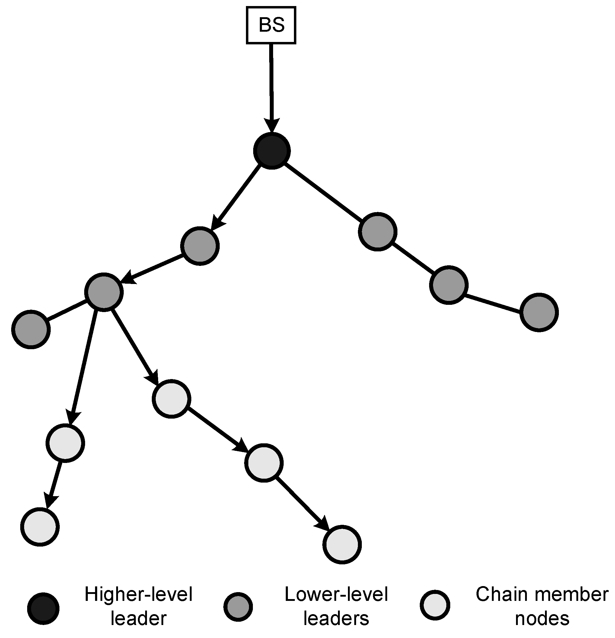
For the proposed multiple chain oriented topology, a three-layer hierarchical management architecture is proposed. Figure 21 represents the relationship between the different entities of the management architecture, namely the manager, the sub-manager and the agent nodes. The manager is in the highest level of the hierarchy and is placed at the BS. The lower-level chain leaders of the proposed topology work as sub-managers, and the chain member nodes work as agent nodes. The sub-managers are used to distribute management functions and collect and collaborate management data. The manager has the global knowledge of the network states and gathers the global knowledge from the underlying network layers and sub-managers.

Figure 21. Different entities of the network management scheme for the proposed topology.

Figure 21. Different entities of the network management scheme for the proposed topology.

The proposed logical topology arranges the nodes into groups of chains and identifies a chain leader for each chain. This allows a subset of nodes to communicate with the sink nodes, conserving energy in the nodes that no longer need to send data to the sinks. Often sink nodes are farther away from many nodes in the network. Chaining procedure abandons these long paths required for communication for smaller hops since nodes will only be communicating with neighbour nodes (except for the chain leaders). Besides energy and bandwidth conservation, there are other advantages of clustering nodes in a WSN. One advantage is that it allows for spatial reuse of resources. If two nodes exist in different non-neighbouring clusters, it may be possible for the two nodes to share the same frequency or time slot. It is also beneficial in the presence of mobility. When using clustering and a node moves, it is often only necessary to update the information in the nodes sharing a cluster with the mobile node; all nodes in the network will not have to be updated. Clustering into chains can also facilitate network management and routing since many implementations require only the chain leader to participate in these functions. In this management architecture, the chain leaders (often called sub-manager) report the data to the manager on behalf of the entire cluster.

Three major aspects of the proposed network management are discussed below, namely fault detection, performance management, and security management.

5.1. Fault Detection

Fault detection is the process by which the network manager identifies a node that is malfunctioning or almost dead and unable to sense or transmit data. If a normal sensor node dies, it does not create much of a problem except decreasing reliability. However, if a chain leader dies, the data of that chain are lost, and in the worst case, such a failure introduces network partition in the system.

In traditional IP networks, the usual way to determine whether a node is working properly is to receive periodic keepalive messages from that node. However, for sensor network such message exchange is very costly. Therefore, fault detection operation in WSNs should be lightweight, and performed using passive information as much as possible.

The fault of normal sensors is detected by the sub-manager (i.e., by the lower-level leaders). If the sensors are supposed to send data periodically, then by analyzing the packets, the lower-level leader can identify the sensor node that is not responding. The lower-level leaders can also miss packets from member nodes caused by collisions. Inside the chain, each sensor maintains the state of its neighbours. If a sensor does not hear from any of its neighbour for a certain period of time, the node informs the lower-level leader about that particular sensor. The lower-level leader and the neighbours maintain a timer T for each of the neighbour sensors. If the lower-level leader or the neighbours hear a transmission from that sensor, then they reset the timer. If the timer of the lower-level leader expires, then it waits before declaring the alarm. If the timer of the neighbour expires, it piggybacks that information in the next data packet. If the lower-level leader receives packets from any of the neighbours of that node without any negative result, the leader waits for another random time. If there is no positive response before the timer expires, or random delay is extended three times, then the leader node generates an alarm, and decides that the node is dead. The leader then informs the manager about the dead node. For event-driven sensor networks, the sensor sends a periodic keepalive message to the sink in the absence of an event.

Lower-level leaders use timer T and reset it when fault detection of lower-level leaders is more important than that of a chain member node. In cases of periodic traffic, the central manager analyzes the packets received by the sink. As the central manager knows the topology of the network, it knows the path of each chain leader to the BS. It maintains two timers ($T_1$ and $T_2$) for each chain leader and for gateway nodes. When the sink receives a packet from that node or through that node, the central manager restarts the timer. If the timer expires, then the central manager suspects that node is dead. As the fault should be detected immediately, the value of $T_1$ should not be very high. When the timer expires, the chain leader sends a query packet to the node and waits for another time $T_2$. If no response is received, it decides that the node is dead.

In event-driven sensor networks, in the absence of events, the chain leaders or gateway nodes send periodic message and the chain leader uses the same timer mechanism to detect faults.

5.2. Performance Management

The performance management of WSNs monitors the performance of the network and keeps resource consumption as low as possible, especially the use of energy. One of the major performance issues of the WSN is event reliability, which is defined as the number of unique data packets received by the sink node. For optimum performance, the management system sets the data generation rate of the sensors and may also keep some nodes in the sleep state and others in the normal live state.

Performance management consists of monitoring network devices and links in order to determine utilization. Utilization may vary depending on the device and link; it may include processing load, network card utilization, packet-forwarding rate, error rate, or packets queued. Monitoring utilization helps to ensure there is available capacity. Monitoring the network performance assists in identifying current and future bottlenecks and aids in capacity planning. Tracking the utilization of network resources by each user is the goal of accounting management. The primary function of this information is to bill users for their use of the network and its resources. This information can be used to establish metrics and quotas. The usage information also helps the network manager to allocate network resources properly. It is also helpful to see typical user behaviour as then atypical behaviour can be identified and addressed. Atypical behaviour may indicate a security breach or intrusion or may be an indication of a future device problem.

5.3. Security Management

Due to the large number of sensor nodes and the broadcast nature of wireless communication, it is usually desirable for BS to broadcast commands and data to sensor nodes. The authenticity of such commands and data is critical for the normal operation of sensor networks. If convinced to accept forged or modified commands or data, sensor nodes may perform unnecessary or incorrect operations and cannot fulfil the intended purposes of the network. Thus, in hostile environments (e.g., battlefield, antiterrorists operations), it is necessary to enable sensor nodes to authenticate broadcast messages received from BSs.

A protocol that can be adopted in the proposed logical topology is SecCOSEN, which has been proposed for authentication and establishing secret keys in WSNs for multiple chain oriented logical topology. SecCOSEN uses partial key pre-distribution and symmetric cryptography techniques. While one version of the SecCOSEN protocol uses shared partial keys in a sensor chain, the other version uses private partial keys. Both versions of SecCOSEN show high resilience to different security attacks. The protocol outperforms other random key pre-distribution protocols as it requires less space, has lower communication overheads, and offers very high session key candidates.

6. Performance Evaluation of the Proposed Topology

Several simulation experiments were carried out to evaluate the performance of the logical topology. The proposed logical topology was used for data collection, and its performance was measured against existing data collection protocols, namely LEACH [41], PEGASIS [40], and COSEN [43].

The simulation program was written in object oriented programming language C++. One hundred sensor nodes were assumed to be randomly distributed in the target field of 100 m × 100 m, and the BS was located at (25, 150). Cartesian coordinates were used to locate the sensor nodes. It was further assumed that each sensor starts with one Joule of initial energy.

In practice it is difficult to model energy expenditure in radio wave propagation. Therefore, in order to measure the energy expenditure in the network, the same simplified radio model used in LEACH and PEGASIS was used. The value of the radio parameters of transmitter and receiver electronics that were used in the simulation are $E_{tx-elec}=E_{Rx-elec}=E_{elec}=50$ nJ/bit. The value of transmit amplifier was assumed to be 100 pJ/bit/$m^2$. It was further assumed that a computation cost of 5 nJ/bit/message would be required to fuse 2000-bit messages. The bandwidth of the channel was set to 1 Mb/s. Thus the total transmission cost for a k-bit message is given by the following equation:

$$\begin{array}{c}\hfill E_{tx}(k,d)=E_{elec}k+k{d}^2\end{array}$$

where d is the distance between sender and receiver measured in meters. In the case of receiving a message, the energy consumption equation is given by the following equation:

$$\begin{array}{c}\hfill E_{rx}\left(k\right)=E_{eleck}\end{array}$$

Multiple runs of the simulation for each protocol were performed and the average value was taken. The metrics that were considered to measure the performance of each protocol were (i) overall energy expenditure in the network; (ii) lifetime of the network; (iii) time to complete a fixed number of operational rounds.

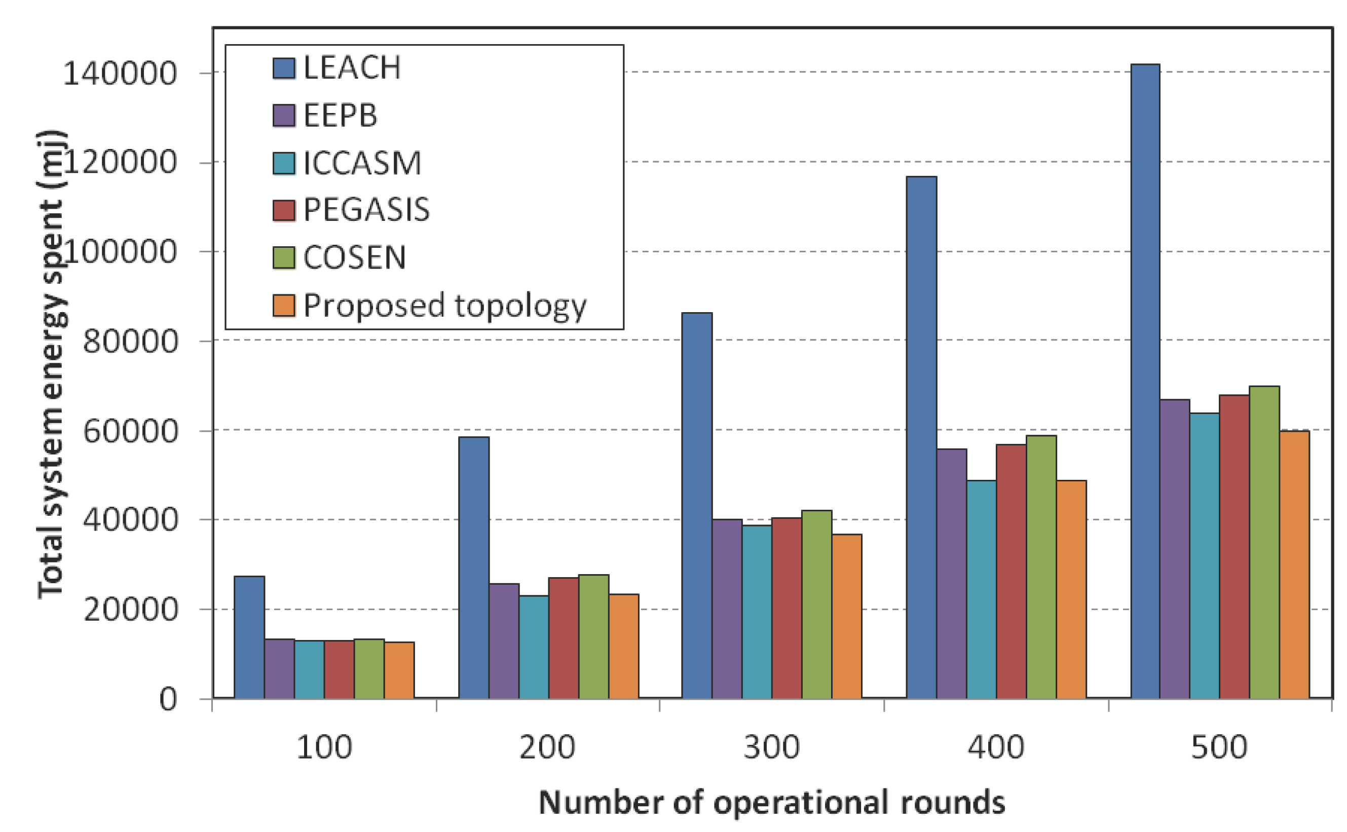
The first experiment measured the total energy consumption by the system varying the number of operational rounds. We measured the total energy consumption in the system after 100, 200, 300, 400 and 500 rounds of operation. As most of the nodes were dying after 500 rounds of operations, we stopped measuring the total energy spent in the system after 500 operation rounds. The total energy spent by the system was calculated by summing up the energy spent by each individual sensor node. Figure 22 shows the results. It is notable that all the chain-based protocols outperform the cluster-based protocol LEACH. PEGASIS was found to be more energy conservative than LEACH and COSEN, however, the proposed topology outperformed PEGASIS by saving more than 10% of total energy for 500 data collection rounds. This is because of the optimal chain creation by the proposed algorithm and the efficient leader selection processes.

Figure 22. Total energy consumption comparison among LEACH, PEGASIS, COSEN, EEPB, ICCASM and the proposed topology.

Figure 22. Total energy consumption comparison among LEACH, PEGASIS, COSEN, EEPB, ICCASM and the proposed topology.

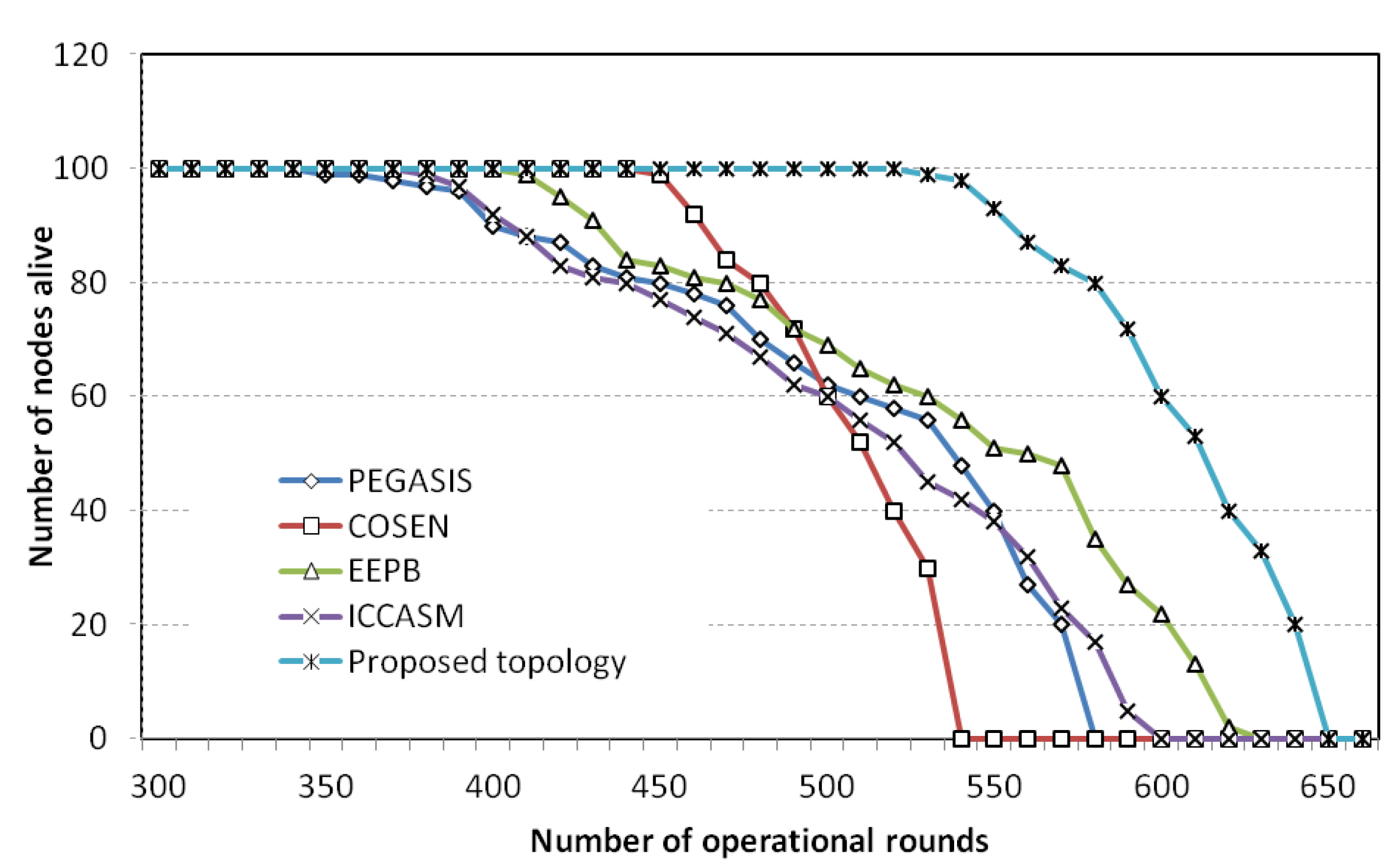
While the proposed topology was the most efficient in total energy consumed, the main success of the proposed topology is the even distribution of energy consumption. Uneven energy consumption by the sensor nodes adversely affects the system lifetime. Figure 23 demonstrates the lifetime comparisons between the proposed topology and the protocols PEGASIS, COSEN, EEPB and ICCASM. The figure shows that the death of the first node in PEGASIS occurs at an early stage compared with COSEN and the proposed topology. For PEGASIS, 10% of the nodes die at around 400 operational rounds, whereas for the proposed topology, 10% of the nodes die at around 550 rounds. Although the final node expiration time is impressive for EEPB, the protocol suffers from uneven energy dissipation. The first node of the protocol EEPB dies only after 410 operational rounds. The protocol ICCASM shows almost similar lifetime patters with the protocol PEGASIS. The main reason the proposed protocol can save energy is to avoid the cross links, which cannot be avoided in PEGASIS, or ICCASM, or in COSEN.

Figure 23. Lifetime comparisons among PEGASIS, COSEN, EEPB, ICCASM, and the proposed topology.

Figure 23. Lifetime comparisons among PEGASIS, COSEN, EEPB, ICCASM, and the proposed topology.

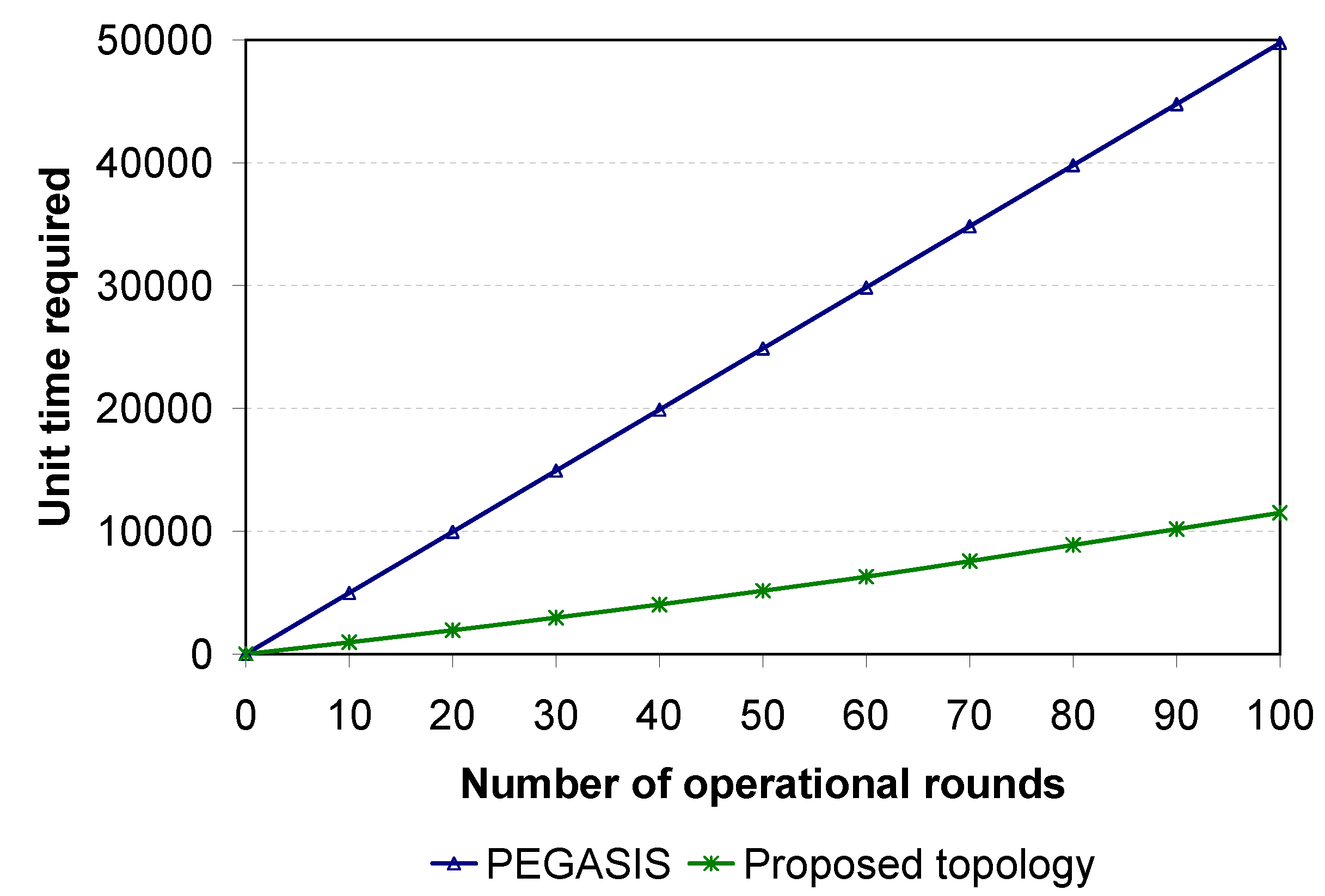
The definitive improvement of the proposed topology over PEGASIS is the latency in data collection. In the simulation, the required amount of time to complete different numbers of operational rounds for PEGASIS and the proposed topology was calculated (Figure 24). The pattern of the time requirement graph suggests that PEGASIS is not suitable for large-scale WSNs due to latency. For 100 operational rounds, the proposed topology requires approximately one-fifth of the time required by PEGASIS.

Figure 24. Latency comparison between PEGASIS and the proposed topology.

Figure 24. Latency comparison between PEGASIS and the proposed topology.

7. Conclusions

This paper presents a multiple chain oriented logical topology for WSNs. The design of the topology is governed by various factors including resource constraints such as energy, time, and computational complexity, as well as networking and architectural factors, and network management issues. Detailed descriptions of the construction of the proposed topology are provided. Moreover, a three-layer hierarchical management architecture is proposed for the multiple chain oriented topology. The network management scheme works in line with the proposed topology for managing different issues such as fault detection, performance management, and security management.

The proposed topology entails three phases: topology formation phase, steady state phase, and topology update phase. While the first phase takes place only once during the initial stage, the remaining two phases continue in rotation. Various issues, such as the optimal number of chains in the system, the optimal number of nodes in a chain, the time when the leader nodes need to be changed, and when the chains should be reconstructed, are described in detail. The communication abstraction describes the process by which sensor nodes send and receive different control messages and sensed data.

In designing the proposed multiple chain oriented topology, it is important to note that reducing the energy consumption will not always result in a longer system lifetime. Instead, balancing resources among sensors and saving energy for those more resource-constrained sensors are very helpful in lengthening the overall system lifetime. The chains of the proposed topology were constructed, and the leader nodes were selected on the basis of this principle.

Simulation results showed excellent results in favour of the proposed logical topology. The proposed logical topology outperformed LEACH, PEGASIS and COSEN not only in total system energy consumption but also in system lifetime. The key reason behind this is the more even distribution of energy consumption. The proposed topology also solves the high delay problem of PEGASIS.

However, there are still some areas where the performances of the proposed logical topology can be enhanced further. These areas may include: (i) the use of node scheduling so that a number of sensor nodes can be turned off while still maintaining the coverage or other user requirements; (ii) the creation of localised chains (where all the chains are restricted in precise areas so no chain crosses any other chain in order to avoid more interferences); and (iii) designing mobile data collectors.