A Framework for Multiple Object Tracking in Underwater Acoustic MIMO Communication Channels

Abstract

This work presents a computational framework for the analysis and design of large-scale algorithms utilized in the estimation of acoustic, doubly-dispersive, randomly time-variant, underwater communication channels. Channel estimation results are used, in turn, in the proposed framework for the development of efficient high performance algorithms, based on fast Fourier transformations, for the search, detection, estimation and tracking (SDET) of underwater moving objects through acoustic wavefront signal analysis techniques associated with real-time electronic surveillance and acoustic monitoring (eSAM) operations. Particular importance is given in this work to the estimation of the range and speed of deep underwater moving objects modeled as point targets. The work demonstrates how to use Kronecker products signal algebra (KSA), a branch of finite-dimensional tensor signal algebra, as a mathematical language for the formulation of novel variants of parallel orthogonal matching pursuit (POMP) algorithms, as well as a programming aid for mapping these algorithms to large-scale computational structures, using a modified Kuck’s paradigm for parallel computation.

1. Introduction

This work formulates a computational framework for the development of efficient algorithms to effect computational signal processing operations to address the problem of electronic surveillance and acoustic monitoring (eSAM) of deep underwater moving objects. From the point of view of computational complexity theory, the combined problem of search, detection, estimation and tracking (SDET) of deep underwater moving objects through active signal sensing is considered an NP-hard problem [1,2,3]. This is in the context of transmitter signal waveform design and signal-to-noise ratio (SNR) optimization. For this reason, large-scale modeling and simulation environments are needed in order to analyze, design and implement high performance computational signal processing algorithms that may provide optimal approximate solutions to this problem. In order to facilitate the exposition of the proposed computational framework, we proceed to simplify the formulation of the SDET problem in the following manner.

Problem formulation: There is a need to develop approximate algorithms for the estimation of the range and speed of deep underwater moving objects to facilitate tracking operations [4,5]. These tracking operations are performed in a communication medium that manifests time-frequency dispersion effects and must be characterized as an acoustic, linear, stochastic (ALS), time-variant channel [6].

To obtain approximate solutions to this simplified SDET problem, we decomposed the problem itself into three main stages: (i) how to characterize the communication channel between the set of signal transmitters, assumed here to be M transmitters, and the set of scattering moving objects; (ii) how to characterize the scattering interaction among the transmitted signals and the scattering moving objects, assumed here to be $K_L$ scattering objects; and (iii) how to characterize the communication channel between the set of scattering moving objects and the set of signal receivers, assumed here to be N signal transducers?

Stages (i) and (iii) were integrated in a unified manner, and the communication channels were modeled as ALS time-variant systems resulting in a MIMO channel characterization formulation. Stage (ii) was addressed using multidimensional, multi-component, polynomial phase (MMPP) signals and operator theoretic properties associated with discrete Cohen distributions (DCDs) under a bidimensional harmonic analysis setting. This approach at solving the SDET problem allowed us to integrate the channel estimation problem of digital communications and the scattering object parameter estimation problem of sensor array signal processing.

This paper presents algorithmic formulations for the solution of the simplified SDET problem using Kronecker products signal algebra (KSA) as the mathematical language to convey our proposed computational signal processing methods in parallel format, which, to the best of our knowledge, are original formulations. Thus, this work extends the work of Li, W.and Preisig, J.C. on the estimation of rapidly time-varying sparse channels by providing a solution to the estimation problem for the multiple-input multiple-output (MIMO) case in parallel form, using Kronecker products signal algebra [7]. The language of Kronecker products has been demonstrated to be a very useful tool for the mathematical formulation of fast unitary transforms. In 1990, Rodríguez, D. co-authored a 52-page tutorial article on a methodology for designing, modifying and implementing Fourier transform algorithms on various architectures using tensor or Kronecker products and an associated class of stride group permutations for numerical data flow management [8].

The results presented here are based on two additional works: first, on the work of Carrascosa, P.C. and Stojanovic, M. on underwater acoustic channel estimation, where they introduce spatial multiplexing to increase the data rate supported by the band-limited restriction of the channel [9,10]; second, on the work of Yatawatta, S. and Petropulu, A. on blind channel estimation, where they allow the users at the transmitter to transmit simultaneously, without any bandwidth restrictions, each user utilizing a single antenna [11]. This work introduces innovation along three main venues: (i) using a mathematical language formulation to describe the processes of channel estimation and multiple object tracking in a unified manner; (ii) developing unique cyclic discrete time-frequency distributions for range-Doppler estimation; and (iii) exploiting the algebraic properties of block circulant structures in order to reduce the overall computational complexity of channel estimation algorithms. We provide in

Table 1. Attributes of selected channel estimation algorithms. MOT, multiple object tracking.

	Algorithms	RTVSC	UWA-MIMO	BCE-MIMO	MOT-MIMO
Features
Authors		Li, W.	Carrascosa, P.C.	Yatawatta, S.	Rodriguez, D.; Aceros, C.;
		Preisig, J.C.	Stojanovic, M.	Petropulu, A.	Valera, J.; Anaya, E.
Reference		[7]	[9]	[11]	Proposed Work
MIMO		×	✓	✓	✓
Formulation
Tracking		✓	✓	×	✓
Capability
Kronecker		✓	×	✓	✓
Products
Formulation
MIMO Parallel		×	×	×	✓
Algorithm
Implementation

a description of the salient attributes of the channel estimation algorithms of these selected works, as well as the salient features of multiple object tracking (MOT) MIMO estimation algorithms presented in this work.

In 1993, Van Loan, C. wrote a now well-known book on computational frameworks for fast Fourier transform algorithms. The book explains how “different FFT algorithms correspond to different factorizations of the discrete Fourier transform (DFT) matrix,” and it shows how computer implementations of FFT algorithms are directly related to their mathematical formulations in Kronecker products notation [12]. Van Loan’s book extended, in a systematic manner, the approach presented in [8] for identifying Kronecker products expressions with computational constructs. In 2006, Franchetti, F. et al., presented a software program generator and optimizer for linear signal transforms, such as the DFT [13]. This language generator was written using the Kronecker products notation formulated in [8]. In 2007, Ali, A. et al. developed a portable framework for FFT algorithms to run on various parallel architectures. The computational framework was also formulated using the language of Kronecker products [14]. In 2008, Rodríguez, D. co-authored an article where a methodology was presented for the high-level partitioning of signal transforms onto distributed hardware architectures using, again, the language of Kronecker products signal algebra [15].

A direct mapping from Kronecker products expressions, which we termed functional primitives, to MATLAB (MATrix LABoratory) pseudocode, was clearly established by Franchetti, F. et al., in 2009, in an article that provides “the techniques needed to implement the discrete Fourier transform (DFT) efficiently on current multicore systems”, and also discusses optimization techniques for good multicore performance [16]. In 2009, Kepner, J. wrote a book for parallel programming in MATLAB, with specific examples of application algorithms written using the open source pMatlab software library [17]. A good feature of this book is how it presents “a more sophisticate model [to] handle hierarchical collections of processors, memories, and networks”.

The rest of this document is structured as follows. Section 2 introduces the concept of delay-Doppler MIMO estimation, describes our original MIMO channel model and presents three matching pursuit algorithm variants for its impulse response function estimation. Section 3 describes Kuck’s paradigm for parallel computation used in our work as the computational model for the implementation of the Kronecker products-based algorithms. Section 4 presents a description of the implementation results obtained from our computational testbed for a particular solution of the simplified SDET problem when we simulate the detection and tracking of two deep underwater objects, at rest or moving at a constant speed. Two acoustic signal transmitters and two acoustic signal receivers are used to actively sense the communication medium. The section also describes an example of deep underwater tracking simulation of ten (10) objects, four (4) of them permanently fixed. Finally, Section 5 provides our conclusions.

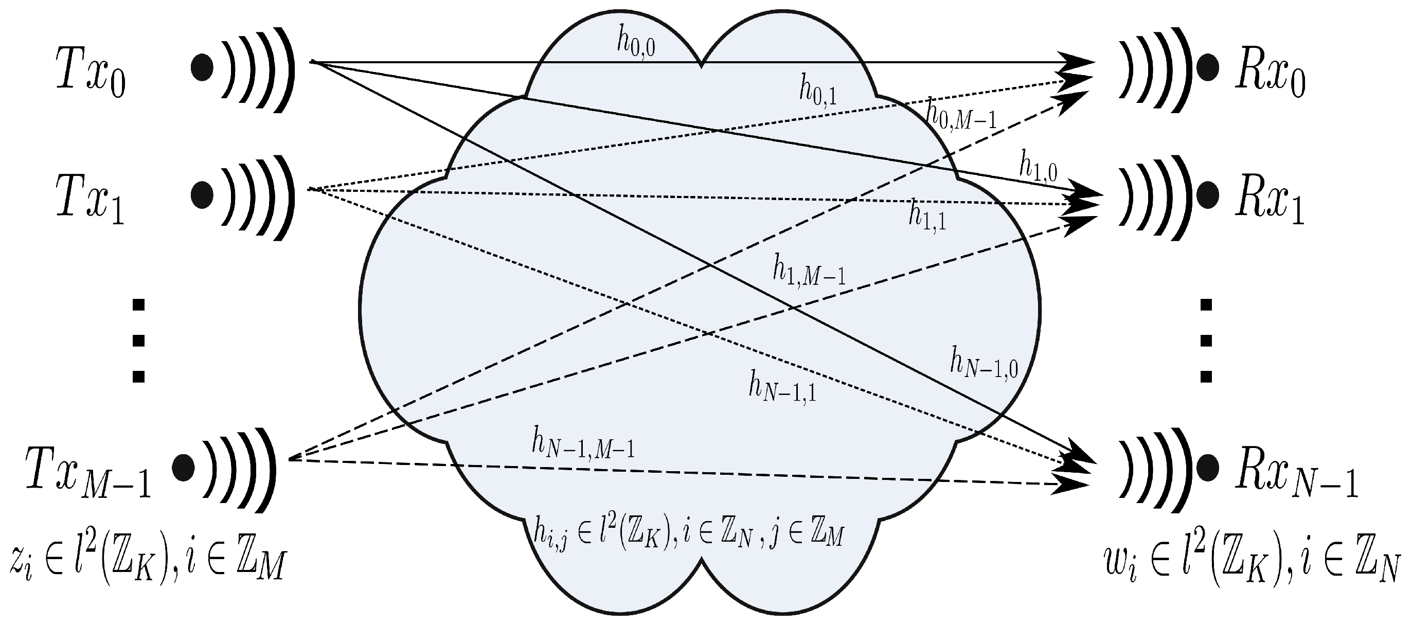
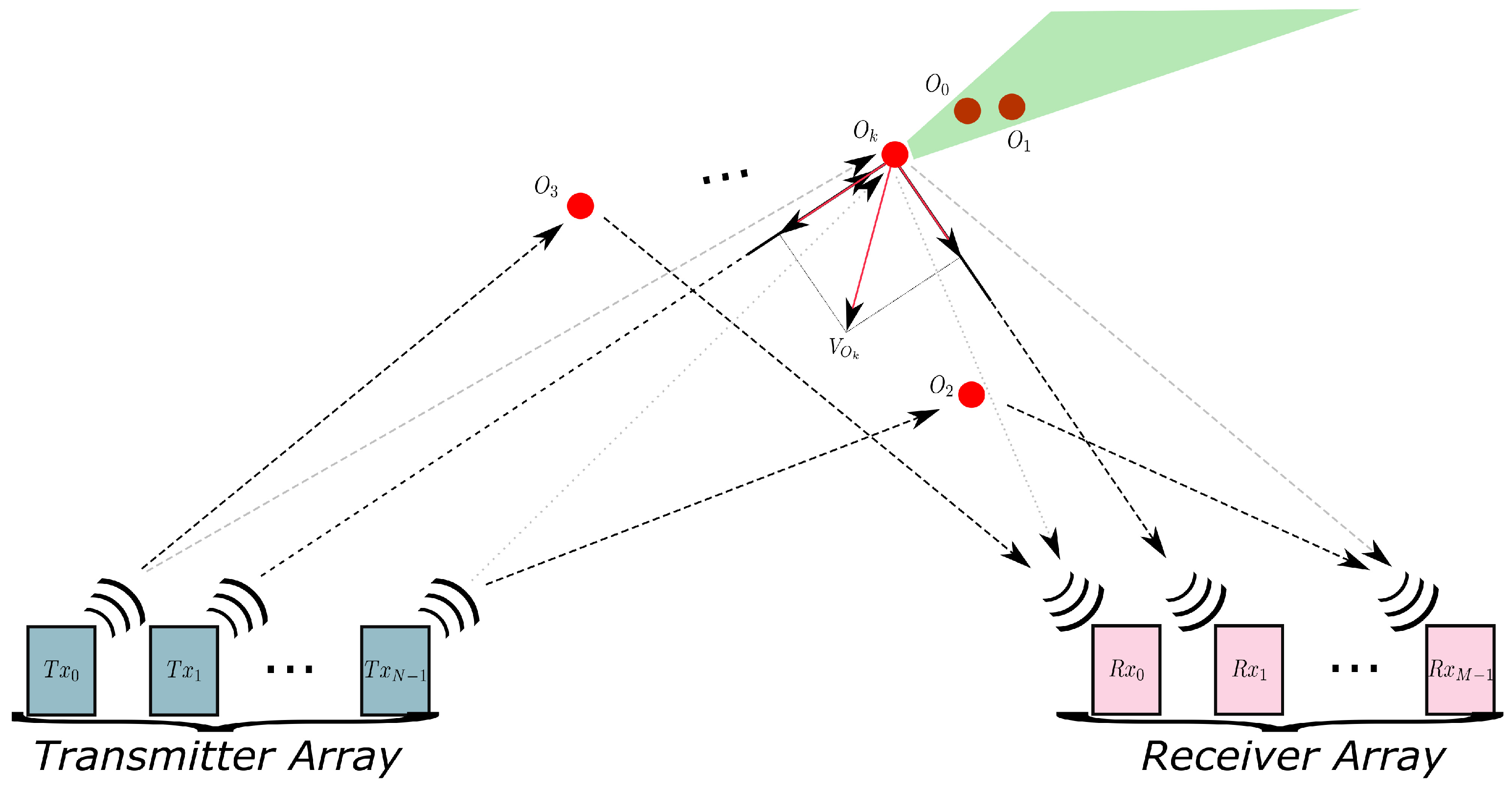
2. Delay-Doppler MIMO Channel Characterization

In this section, we formulate the characterization of MIMO acoustic, linear, stochastic (ALS), time-variant systems and describe a set of matching pursuit greedy algorithms to estimate MIMO channel parameters. The characterizing channel function used in this work is the delay-Doppler spread function $U(\xi ,\nu )$ [18]. This function plays the role of surrogate function for the input-delay spread function; that is, for the impulse response function $h(t,\xi )$ of acoustic linear stochastic (ALS) channels [19].

The parameters to be estimated are time-delays and the Doppler shifts associated with the delay-Doppler spread function. This estimation work must be carried out in a fraction of the time corresponding to the channel’s coherence time, $T_C$; that is, the time period during which the impulse response function is assumed to be time-translation invariant. This approach for channel parameter estimation is done under a multiple-input multiple-output (MIMO) system assumption. Thus, we consider M transmitter transducers and N receiver transducers in a MIMO system scenario. It is possible in this scenario that a determined number of scatterers, L, may be present between the transmit and receive transducers. We assume that some scatterers may be in motion, moving at a constant speed. These movements introduce Doppler effects, which are manifested as frequency shifts acting over each copy of the transmitted signals $z_m\left(t\right)$ associated with each scattering point $P_l$, $l\in {\mathbb{Z}}_L$, in motion.

An abstract depiction of the bistatic sonar nature of our proposed deep underwater multiple object tracking scenario is given in Figure 1. Under the MIMO assumption, we can express each received signal $w_n\left(t\right)$ as the sum of L copies of each transmitted signal $z_m\left(t\right)$, time delayed by ${\xi }_l$, shifted by its respective Doppler frequency ${\nu }_l$ and scaled by an attenuation factor ${\alpha }_l$.

We define the following expression:

$${\sigma }_{l,m,n}\left(t\right)={\alpha }_{l,m,n}{z}_m(t-{\xi }_{l,m,n})e^{+j2\pi t{\nu }_{l,m,n}}.$$

(1)

Thus, we obtain the following result for each received signal:

$${\displaystyle w_n\left(t\right)=\sum _{m\in {\mathbb{Z}}_M}\sum _{l\in {\mathbb{Z}}_L}{\sigma }_{l,m,n}\left(t\right)+\eta \left(t\right),n\in {\mathbb{Z}}_N,}$$

(2)

where $t\in \mathbb{R}$ and $w,z\in L^2\left(\mathbb{R}\right)$. Here, ${\alpha }_{l,m,n}\in \mathbb{C}$ is the attenuation factor ${\alpha }_l$ associated with each input signal $z_m\left(t\right)$ and received signal $w_n\left(t\right)$. The parameters ${\xi }_{l,m,n},{\nu }_{l,m,n}\in \mathbb{R}$ are the time delay and Doppler shift associated with each scatterer $l\in {\mathbb{Z}}_L$, transmitter $m\in {\mathbb{Z}}_M$ and receiver $n\in {\mathbb{Z}}_N$. The parameters ${\xi }_{0,m,n}$ and ${\nu }_{0,m,n}$ are set to zero, for line of sight (L.o.S.) consideration.

The signal $\eta \left(t\right)$ is a real-valued, independent, wide-sense, stationary, Gaussian stochastic process that represents the channel noise. This approach captures the more important aspects of a physical realization of a deep underwater ALS MIMO channel. Under the MIMO assumption, we can obtain the impulse response function of the deep underwater ALS channel by substituting each input signal $z_m\left(t\right)$ with the impulse function ${\delta }_m\left(t\right)$ in Equation (2). We proceed to define the following expression:

$${\psi }_{l,m,n}\left(t\right)={\alpha }_{l,m,n}{\delta }_m(t-{\xi }_{l,m,n})e^{+j2\pi t{\nu }_{l,m,n}}.$$

(3)

Thus, we obtain:

$${\displaystyle h_{n,m}(t,\xi )=\sum _{m\in {\mathbb{Z}}_M}\sum _{l\in {\mathbb{Z}}_L}{\psi }_{l,m,n}+\eta \left(t\right),n\in {\mathbb{Z}}_N,}$$

(4)

where $t\in \mathbb{R}$ and $w,z\in L^2\left(\mathbb{R}\right)$. Here, $h_{n,m}(t,\xi )$ (kernel function) is the time-variant impulse response between the transmitter $m\in {\mathbb{Z}}_M$ and the receiver $n\in {\mathbb{Z}}_N$.

As previously stated, the MIMO channel model formulated in this work has M transmitter transducers and N receiver transducers. Equation (5) presents the input-output relation of our MIMO channel model.

From Figure 2, we may obtain, after a series of algebraic manipulations, using concepts from our proposed computational framework, the following channel input/output relationship:

$$\begin{array}{c}\hfill {\displaystyle \mathbf{w}=\left[\underset{i\in {\mathbb{Z}}_M}{⨆}\left(\underset{j\in {\mathbb{Z}}_N}{⨁}\mathcal{C}\left\{z_i\right\}\right)\right]\left[\underset{i\in {\mathbb{Z}}_N}{\bigvee }\left(\underset{j\in {\mathbb{Z}}_M}{\bigvee }{h}_{i,j}\right)\right]=}\\ \hfill \left[\underset{i\in {\mathbb{Z}}_M}{⨆}(I_N\otimes \mathcal{C}\left\{z_i\right\})\right]\left[\underset{i\in {\mathbb{Z}}_N}{\bigvee }\left(\underset{j\in {\mathbb{Z}}_M}{\bigvee }{h}_{i,j}\right)\right]=\mathbf{Z}\mathbf{h},\end{array}$$

(5)

where $z_i\in l^2\left({\mathbb{Z}}_K\right),i\in {\mathbb{Z}}_M$ is the i-th transmitted signal, $h_{i,j}\in l^2\left({\mathbb{Z}}_K\right),i\in {\mathbb{Z}}_N,j\in {\mathbb{Z}}_M$ is the $ij$-th impulse response, $w_i\in l^2\left({\mathbb{Z}}_K\right),i\in {\mathbb{Z}}_N$ is the i-th received signal, ⊗ is the Kronecker products operator, ⋁ is the vertical matrix concatenation operator, ⨆ is the horizontal matrix concatenation operator, $\mathbf{Z}\in l^2({\mathbb{Z}}_{KN}\times {\mathbb{Z}}_{KMN})$ is the input matrix, $\mathbf{h}\in l^2\left({\mathbb{Z}}_{KMN}\right)$ is the impulse response channel vector, $\mathbf{w}\in l^2\left({\mathbb{Z}}_{KN}\right)$ is the output vector and $\mathcal{C}$ is the circulant operator. We have taken advantage of the coherent condition of the channel and have invoked the properties of the convolution operation. This MIMO system model formulation allows the study of filter bank multi-carrier communication, partial FFT demodulation and waveform diversity design [20,21,22,23]. While in the channel sounding mode, a series of predefined pulses $z_i,i\in {\mathbb{Z}}_M$ is transmitted [24]. These pulses are compared with the received signals $w_j,j\in {\mathbb{Z}}_N$ for characterizing the MIMO channel using the inverse relation shown in Equation (6).

$$\mathbf{h}={\mathbf{Z}}^{†}\mathbf{w},$$

(6)

where $\mathbf{Z}\in l^2({\mathbb{Z}}_{KN}\times {\mathbb{Z}}_{KMN})$ is the signal input matrix, $\mathbf{h}\in l^2\left({\mathbb{Z}}_{KMN}\right)$ is the channel impulse response vector and $\mathbf{w}\in l^2\left({\mathbb{Z}}_{KN}\right)$ is the signal output vector [25]. It is important to point out that to arrive at the mathematical formulation for the MIMO channel input/output system configuration, although not quite difficult, is an intricate and laborious procedure.

We illustrate this procedure by describing in some detail the mathematical formulations for the SISO, MISO and SIMO channel input/output configurations that we first derived in order to arrive at our proposed MIMO channel model system configuration [26].

2.1. SISO, MISO and SIMO Channel Configurations

To arrive at our MIMO channel model system configuration, we start by presenting the SISO, MISO and SIMO configurations. The idea behind this approach is to visualize the algebraic structures in each case. Each configuration has a particular matrix-vector formulation. These formulations allow us to develop data structures and procedures appropriate to address the efficient channel estimation problem. Another important objective in this section is to demonstrate the importance of Kronecker products signal algebra in matrix structure manipulation. Regularities in the matrix structures can be exploited for improving channel estimation algorithms. This work exploits the matrix-vector formulations and sparsity properties; however, many other regularities and symmetries can be identified and reviewed to develop new algorithms.

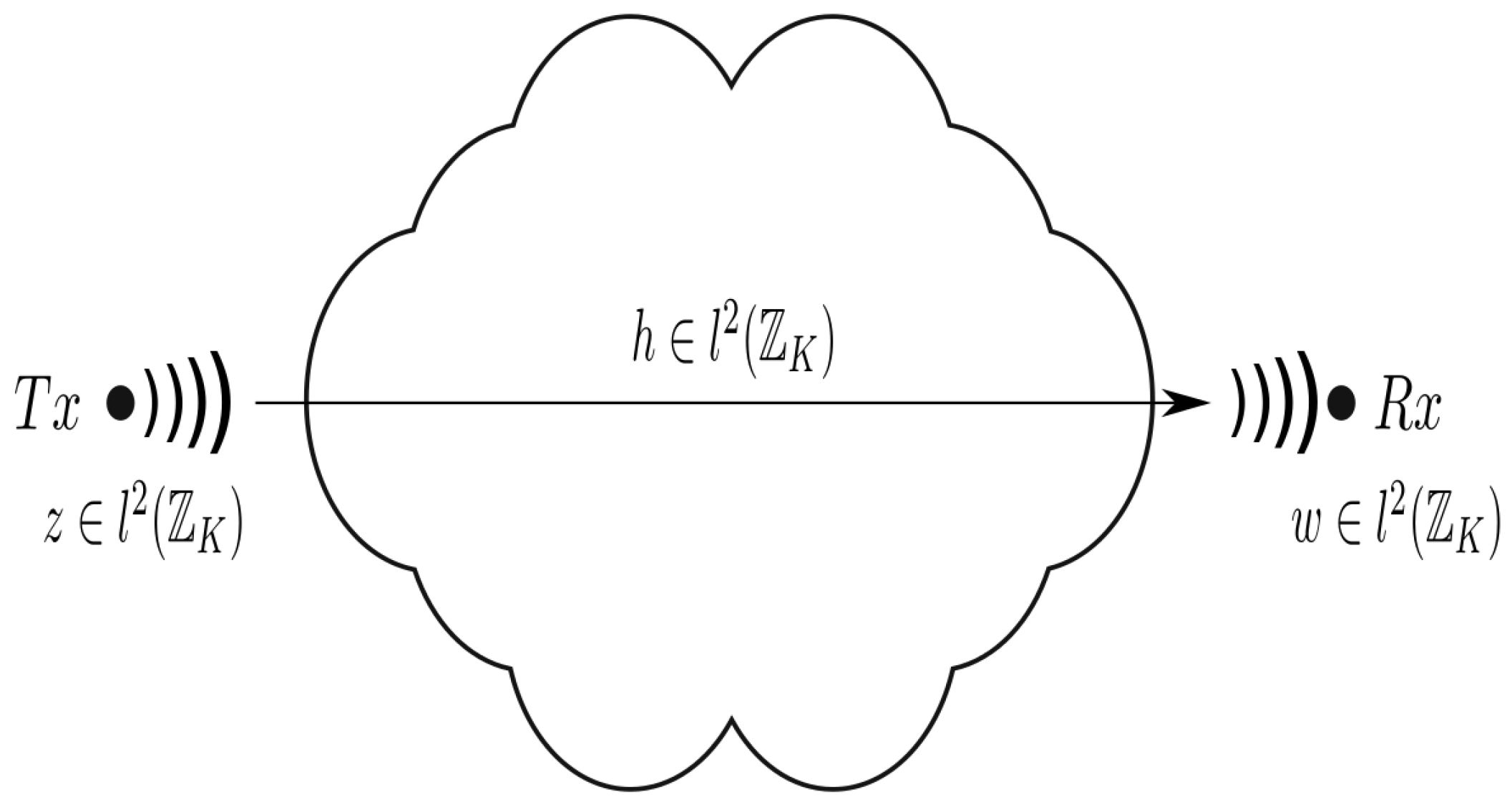
2.1.1. SISO Configuration

The SISO configuration has just one transmitter transducer and one receiver transducer. Equation (7) shows its input-output relationship.

$$w=z{⊛}_{K}h=\mathcal{C}\left\{z\right\}h=\mathbf{Z}h,\mathbf{Z}\in l^2({\mathbb{Z}}_K\times {\mathbb{Z}}_K),$$

(7)

where $z\in l^2\left({\mathbb{Z}}_K\right)$ is the transmitted signal, $h\in l^2\left({\mathbb{Z}}_K\right)$ is the impulse response function of the channel, $w\in l^2\left({\mathbb{Z}}_K\right)$ is the received signal, ${⊛}_K$ is the cyclic convolution operator of order K and $\mathcal{C}$ is the circulant operator. Equation (7) shows a typical input-output relationship for a linear and time-invariant system, also known as a discrete-time filter.

Figure 3 illustrates an SISO channel model system. The matrix-vector representation of the configuration is presented in Equation (8), which shows the first relevant matrix structure of our MIMO channel model configuration, known as a circulant matrix:

$$\left[\begin{array}{c}w\left[0\right]\\ w\left[1\right]\\ ⋮\\ w[K-2]\\ w[K-1]\end{array}\right]=\left[\begin{array}{cccc}z\left[0\right]& z[K-1]& \cdots & z\left[1\right]\\ z\left[1\right]& z\left[0\right]& \cdots & z\left[2\right]\\ ⋮& ⋮& \ddots & ⋮\\ z[K-2]& z[K-3]& \cdots & z[K-1]\\ z[K-1]& z[K-2]& \cdots & z\left[0\right]\end{array}\right]\left[\begin{array}{c}h\left[0\right]\\ h\left[1\right]\\ ⋮\\ h[K-2]\\ h[K-1]\end{array}\right].$$

(8)

The computational complexity, under the direct computation approach, associated with this configuration is $\mathbf{O}\left(K^2\right)$, and it is given by the complexity of the inverse operator acting over the matrix $\mathbf{Z}$ of dimension $K\times K$ and the complexity of the matrix-vector product of the vector w, of length K. Therefore, the dominant complexity is $\mathbf{O}\left(K^2\right)$, where K is the number of samples in the impulse response $h\left[k\right],k\in {\mathbb{Z}}_K$.

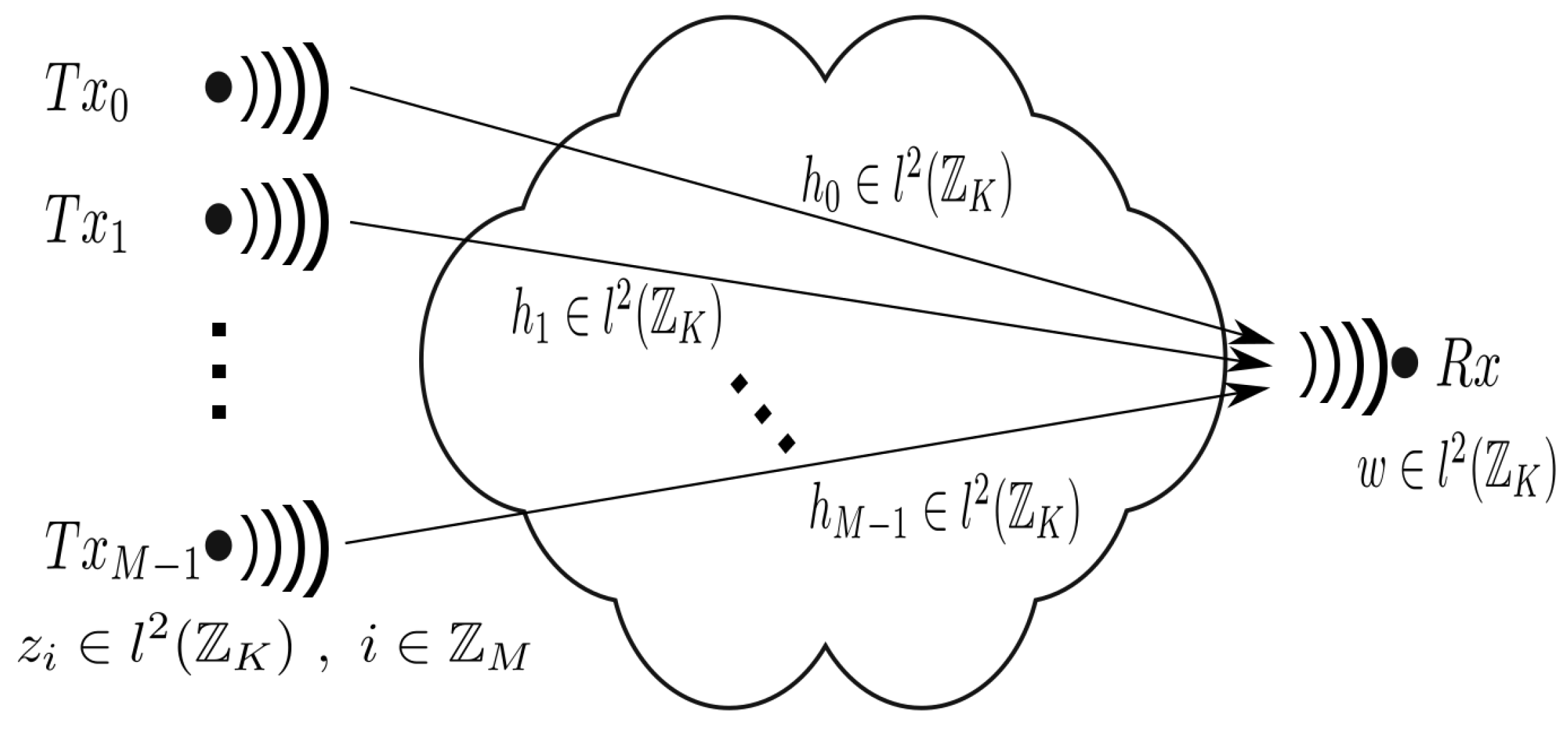
2.1.2. MISO Configuration

The MISO configuration has M transmitter transducers and just one receiver transducer. Equation (9) shows its input-output relationship.

$${\displaystyle w=\sum _{i\in {\mathbb{Z}}_M}{z}_i{⊛}_K{h}_i=\left(\underset{i\in {\mathbb{Z}}_M}{⨆}\mathcal{C}\left\{z_i\right\}\right)\left(\underset{i\in {\mathbb{Z}}_M}{\bigvee }{h}_i\right)=\mathbf{Z}\mathbf{h},}$$

(9)

where $z_i\in l^2\left({\mathbb{Z}}_K\right)$ is the i-th transmitted signal, $h_i\in l^2\left({\mathbb{Z}}_K\right)$ is the i-th impulse response, $w\in l^2\left({\mathbb{Z}}_K\right)$ is the received signal, ${⊛}_K$ is the cyclic convolution operator of order K, ⨆ is the horizontal matrix concatenation operator, ⋁ is the vertical matrix concatenation operator, $\mathbf{Z}\in l^2({\mathbb{Z}}_K\times {\mathbb{Z}}_{KM})$ is the input channel matrix, $\mathbf{h}\in l^2\left({\mathbb{Z}}_{KM}\right)$ is the impulse response channel vector and $\mathcal{C}$ is the circulant operator. Figure 4 illustrates the MISO channel model system. A matrix-vector representation for this model is shown in Equation (10).

$$\left[\begin{array}{c}w\left[0\right]\\ w\left[1\right]\\ ⋮\\ w[K-2]\\ w[K-1]\end{array}\right]=\left[\begin{array}{ccccccc}{z}_0\left[0\right]& \cdots & z_0\left[1\right]& \cdots & z_{M-1}\left[0\right]& \cdots & z_{M-1}\left[1\right]\\ z_0\left[1\right]& \cdots & z_0\left[2\right]& \cdots & z_{M-1}\left[1\right]& \cdots & z_{M-1}\left[2\right]\\ ⋮& \ddots & ⋮& \cdots & ⋮& \ddots & ⋮\\ z_0[K-2]& \cdots & z_0[K-1]& \cdots & z_{M-1}[K-2]& \cdots & z_{M-1}[K-1]\\ z_0[K-1]& \cdots & z_0\left[0\right]& \cdots & z_{M-1}[K-1]& \cdots & z_{M-1}\left[0\right]\end{array}\right]\left[\begin{array}{c}{h}_0\left[0\right]\\ ⋮\\ h_0[K-1]\\ ⋮\\ h_{M-1}\left[0\right]\\ ⋮\\ h_{M-1}[K-1]\end{array}\right].$$

(10)

The computational complexity, under direct computation approach, associated with the MISO channel estimation problem is $\mathbf{O}({\left(KM\right)}^3+2K^3{M}^2))=\mathbf{O}({\left(KM\right)}^3)$, and it is given by the complexity of the pseudo-inverse operator acting over the matrix $\mathbf{Z}$ of dimension $K\times KM$ and the complexity of the matrix-vector product of the vector $\mathbf{h}$, of length $KM$. Therefore, the dominant complexity is $\mathbf{O}({\left(KM\right)}^3)$, where K is the number of samples in the impulse response $h\left[k\right],k\in {\mathbf{Z}}_K$, and M is the number of transmitter transducers.

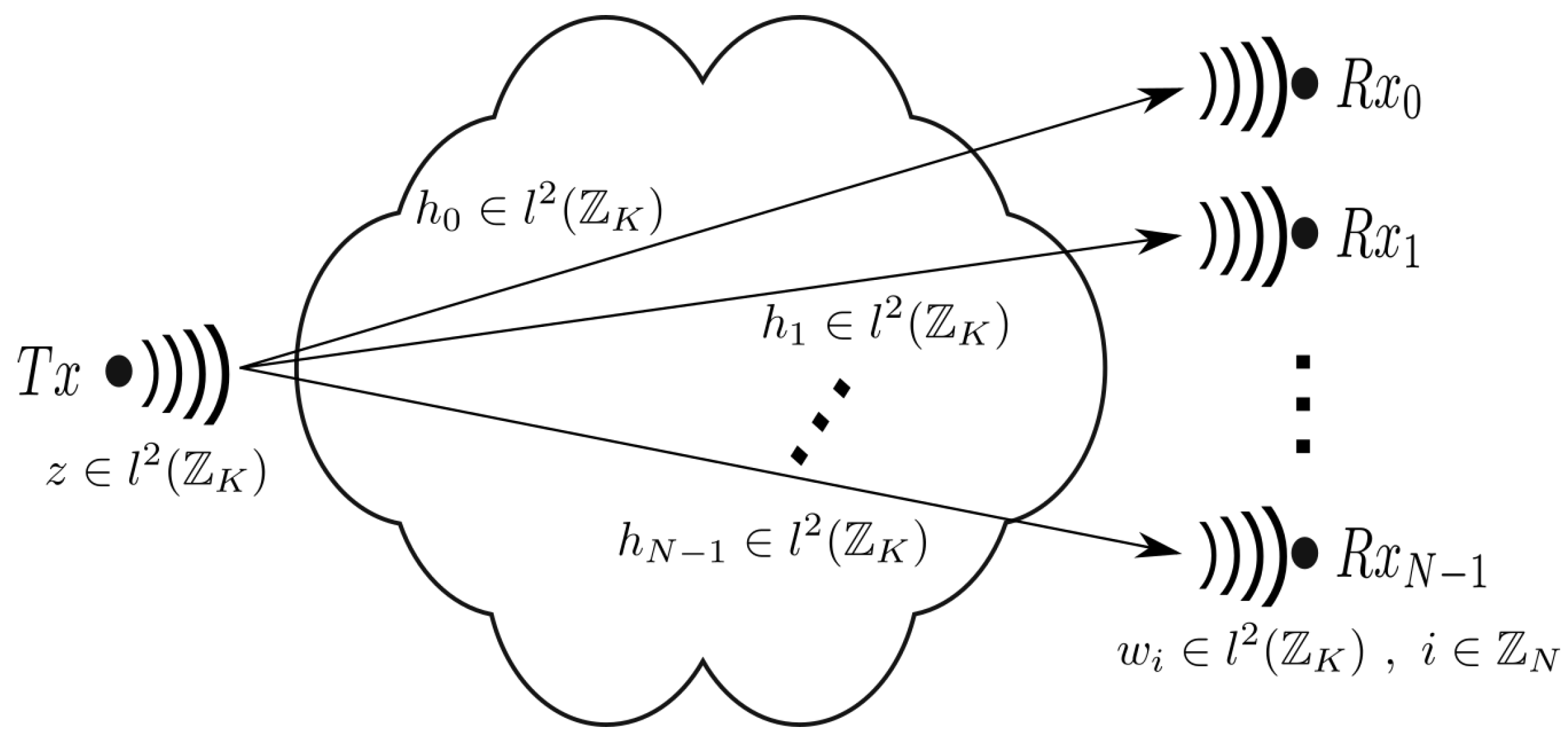
2.1.3. SIMO Configuration

The SIMO configuration has just one transmitter transducer and N receiver transducers. Equation (11) shows its input-output relationship.

$${\displaystyle \mathbf{w}=\underset{i\in {\mathbb{Z}}_N}{\bigvee }z{⊛}_K{h}_i=\left(\underset{i\in {\mathbb{Z}}_N}{⨁}\mathcal{C}\left\{z\right\}\right)\left(\underset{i\in {\mathbb{Z}}_N}{\bigvee }{h}_i\right)=(I_N\otimes \mathcal{C}\left\{z\right\})\left(\underset{i\in {\mathbb{Z}}_N}{\bigvee }{h}_i\right)=\mathbf{Z}\mathbf{h},}$$

(11)

where $z\in l^2\left({\mathbb{Z}}_K\right)$ is the transmitted signal, $h_i\in l^2\left({\mathbb{Z}}_K\right),i\in {\mathbb{Z}}_N$, is the i-th impulse response, $w_i\in l^2\left({\mathbb{Z}}_K\right),i\in {\mathbb{Z}}_N$, is the i-th received signal, ${⊛}_K$ is the cyclic convolution operator of order K, ⋁ is the vertical matrix concatenation operator, $\mathbf{Z}\in l^2({\mathbb{Z}}_{KN}\times {\mathbb{Z}}_{KN})$ is the input channel matrix, $\mathbf{h}\in l^2\left({\mathbb{Z}}_{KN}\right)$ is the impulse response channel vector, $\mathbf{w}\in l^2\left({\mathbb{Z}}_{KN}\right)$ is the output vector and $\mathcal{C}$ is the circulant operator. Figure 5 illustrates the SIMO model system. A matrix-vector representation is shown in Equation (12).

$$\left[\begin{array}{c}{w}_0\left[0\right]\\ w_0\left[1\right]\\ ⋮\\ w_0[K-2]\\ w_0[K-1]\\ ⋮\\ w_{N-1}\left[0\right]\\ w_{N-1}\left[1\right]\\ ⋮\\ w_{N-1}[K-2]\\ w_{N-1}[K-1]\end{array}\right]=\left[\begin{array}{ccccccccc}z\left[0\right]& z[K-1]& \cdots & z\left[1\right]& \cdots & 0& 0& \cdots & 0\\ z\left[1\right]& z\left[0\right]& \cdots & z\left[2\right]& \cdots & 0& 0& \cdots & 0\\ ⋮& ⋮& \ddots & ⋮& \cdots & ⋮& ⋮& \ddots & ⋮\\ z[K-2]& z[K-3]& \cdots & z[K-1]& \cdots & 0& 0& \cdots & 0\\ z[K-1]& z[K-2]& \cdots & z\left[0\right]& \cdots & 0& 0& \cdots & 0\\ ⋮& ⋮& ⋮& ⋮& \ddots & ⋮& ⋮& ⋮& ⋮\\ 0& 0& \cdots & 0& \cdots & z\left[0\right]& z[K-1]& \cdots & z\left[1\right]\\ 0& 0& \cdots & 0& \cdots & z\left[1\right]& z\left[0\right]& \cdots & z\left[2\right]\\ ⋮& ⋮& \ddots & ⋮& \cdots & ⋮& ⋮& \ddots & ⋮\\ 0& 0& \cdots & 0& \cdots & z[K-2]& z[K-3]& \cdots & z[K-1]\\ 0& 0& \cdots & 0& \cdots & z[K-1]& z[K-2]& \cdots & z\left[0\right]\end{array}\right.\left[\begin{array}{c}{h}_0\left[0\right]\\ h_0\left[1\right]\\ ⋮\\ h_0[K-2]\\ h_0[K-1]\\ ⋮\\ h_{N-1}\left[0\right]\\ h_{N-1}\left[1\right]\\ ⋮\\ h_{N-1}[K-2]\\ h_{N-1}[K-1]\end{array}\right]$$

(12)

The computational complexity, under the direct computation approach, associated with the SIMO problem, is bounded by $\mathbf{O}({\left(KN\right)}^3+2{\left(KN\right)}^3)=\mathbf{O}({\left(KN\right)}^3+2{\left(KN\right)}^3)$, and it is given by the complexity of the pseudo-inverse operator acting over the matrix $\mathbf{Z}$, of order $KN\times KN$, and the complexity of the matrix-vector product of the vector h, of length $KN$. Therefore, the dominant complexity is $\mathbf{O}({\left(KN\right)}^3)$, where K is the number of samples in the impulse response function $h\left[k\right],k\in {\mathbb{Z}}_K$, and N is the number of receiver transducers.

Three matching pursuit algorithm variants were implemented in this work: basic, orthogonal and order-recursive least-square matching pursuit. Basic matching pursuit (BMP) is the most simple implementation of these algorithms. BMP chooses the maximum projection (inner product) of the column set of $\mathbf{Z}$ on the output vector w and extracts the corresponding contribution of each maximum on w. The orthogonal matching pursuit variant adds a new stage to the estimation process. After each iteration, it recalculates all of the ${\lambda }_i$ coefficients associated with each chosen $c_i$ column. This is to force the orthogonal condition on the $\mathbf{w}$ residual vector on the subspace spanned by $c_i$ selected columns.

The process of selecting the columns is similar to the process used in the basic matching pursuit variant. In the order-recursive least-square matching pursuit algorithm variant, the method of selecting the columns is improved in the following manner. Each column is chosen such that it minimizes the residual value of the $\mathbf{w}$ vector. Therefore, each column is chosen considering the previous set of chosen columns for minimizing the $\mathbf{w}$ residual vector, in order to calculate the ${\lambda }_i$ coefficients, so that it is similar to the former algorithm variant. These coefficients provide a guide for the stopping criteria, as pertaining to residual errors, the channel impulse response formulation and the overall performance of the algorithms.

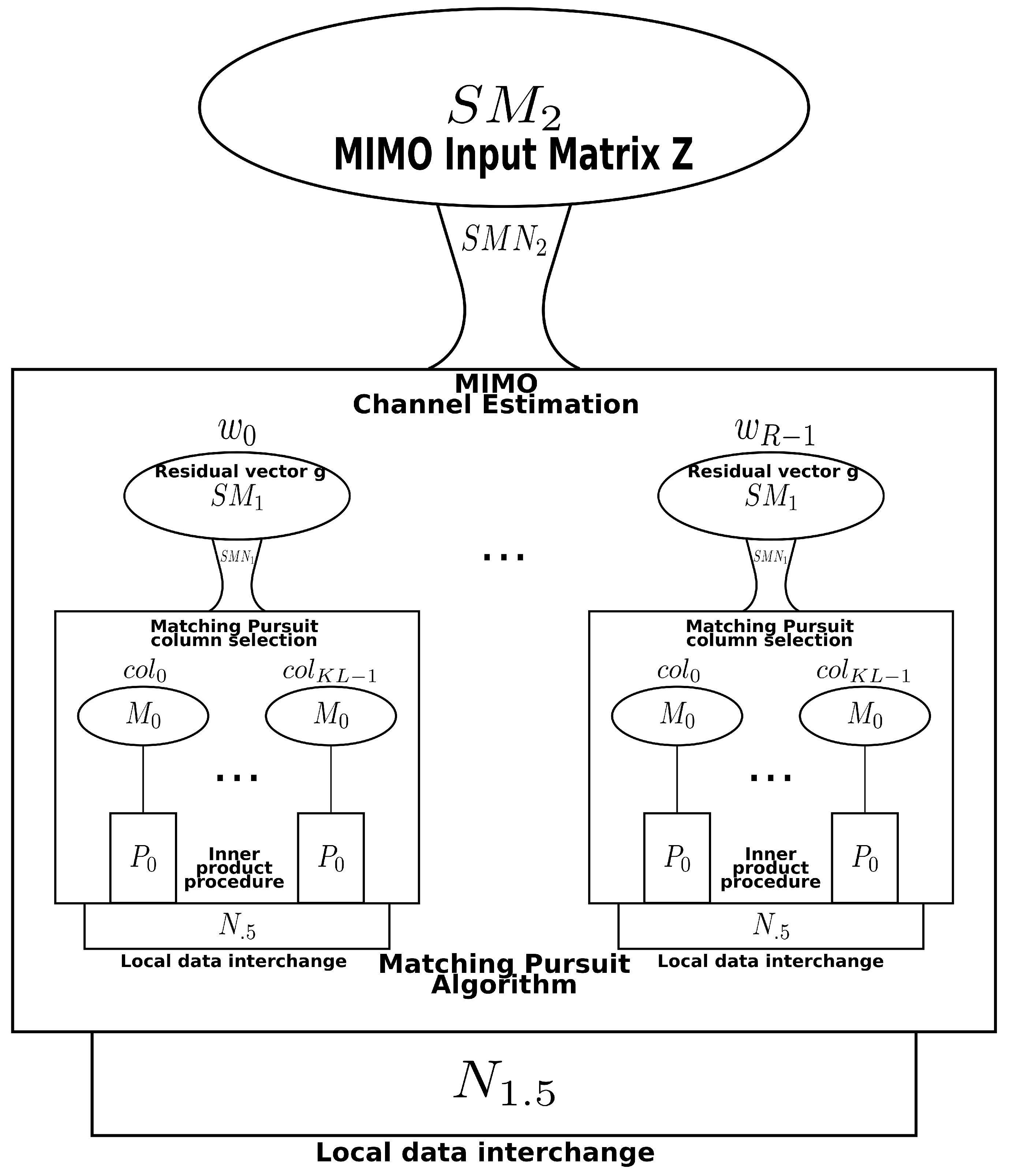
3. Kuck’s Paradigm of Computation

David Kuck presented an abstract manner to represent parallel computational structures [27]. This methodology of representation may be related to the parallel random machine model (PRAM) used to describe an abstract parallel machine, even though our formulation is a more sophisticated model. The goal of a parallelization effort is to reduce the overall computation time by distributing a computational task among available processors.

As its name indicates, the PRAM was intended as the parallel-computing analogy to the random-access machine (RAM). Like random access machine (RAM) models that are used by sequential algorithm designers to model algorithmic performance, the PRAM is used by parallel algorithm designers to model parallel algorithmic performance (such as time complexity, where the number of processors is a parameter). PRAM used the concept of shared memory to avoid the communication problem in message passing interface (MPI) models. The complexity is expressed as a function of the dimension of input set N and the number of processors $Ncpus$.

Kuck’s approach creates a hierarchical structure to represent in a parallel manner the execution of an algorithm. This hierarchical structure reflects the connection between the computing units and shared memory stages. Each level is tagged with a specific label, like “1.5”. This representation approach is sufficiently abstract to allow implementations in a wide spectrum of modern architectures. Figure 6 illustrates Kuck’s diagram representation of the parallel MIMO ALS estimation problem [27]. In this figure, Level 0 represents independent memory units, $M_0$ and uniprocessors $P_0$, which contain registers and caches for fast access to frequently-used data. At level $0.5$, these units are interconnected with a network $N_{0.5}$, generally a bus, mesh, hypercube, shuffle or other mechanism of data interchange. This network provides communication between processors, but does not provide shared memory. Therefore, a protocol for message passing is necessary. The first level of shared-address memory space is $S{M}_1$. The communication between the processors in Level 0 and $S{M}_1$ is managed by $SM{N}_1$. There exists a great difference between direct access to memory via $SM{N}_1$ and indirect access to memory via $N_{0.5}$. The difference is appreciated in the poor performance produced by the indirect access to memory. Now, we can apply a recursive principle to generate new levels.

The algorithmic formulations for solving the SDET problem were implemented in the pMatlab and Parallel Computing Toolbox (PCT) programming environments for MATLAB. These MATLAB parallel programming environments allowed us to conduct detailed computational complexity analysis on the mapping of Kronecker product-based algorithmic formulations to modeled distributed and shared memory structures (see Algorithm 1 and

Table 2. Complexity of matching pursuit (MP) algorithm variants. K = window length, D = number of delays, L = the Doppler shifts, M = number of transmitters, N = number of receivers and I = algorithm iterations.

MP Variant	Alg.Type	Computational Complexity
Basic MP	Greedy	$\mathbf{O}\left(MNDL{I}^2\right)$
Orthogonal MP	Greedy	$\mathbf{O}({\left(MNDL\right)}^2$$+MNDL{I}^2)$
Order Recur-sive LS-MP	Greedy	$\mathbf{O}({\left(MNDL\right)}^2$$+MNDL{I}^2)$
Direct Computation	Pseudo Inverse	$\mathbf{O}({\left(KMNDL\right)}^3)$

).

Algorithm 1: Matching pursuit algorithmic core. Distributed max projection.

1: mapP = map([Ncpus 1],{}, [0:Ncpus-1]); % mapping design $\to {\mathcal{C}}^{V\times P(D\times L)}$ 2: proj=zeros(rows,1,mapP); % $proj:{\mathcal{C}}^{V\times P(D\times L)}$ 3: p = local(proj) % $p\leftarrow proj.loc$ 4: r = local(R); % $r\leftarrow R.loc$ (Scattering Operation) 5: p = ((r´ * g).ˆ2) ./ diag(r´ * r); % local computation 6: proj = put_local(p); % $proj.loc\leftarrow p$ 7: proj = agg(proj); % gathering 8: [Max,column] = max(proj); % getting result

4. Simplified SDET Implementation Results

The MIMO channel configuration used in our testbed experiments is presented in Figure 7. Our experimental results show that the order recursive least square matching pursuit (ORLSMP or OLS, for short) algorithm performs best for MIMO channel estimation. Figure 8 and Figure 9 depict the result of MIMO channel estimation simulations using the three matching pursuit algorithms previously discussed. In each figure, the first graph, from top to bottom, is the given delay-Doppler spread function $U(\xi ,\nu )$ for each MIMO channel link to be estimated. The next graph shows the result of the MIMO channel link estimation using the ORLSMP algorithm, demonstrating its best performance by identifying all tracking objects. The graph that follows shows the results of the orthogonal matching pursuit (OMP) algorithm, which is unable to track all moving objects. Finally, the last graph in each figure shows the results of the basic matching pursuit (BMP) algorithm, which runs very quickly; however, it exhibits a very poor moving object tracking performance.

Table 3. Time performance of MIMO matching pursuit algorithms. BMP, basic matching pursuit.

512	OLS0	OLS1	pOLS	OMP0	OMP1	pOMP	BMP0	BMP1	pBMP
SERIAL	2.0459		2.0459	0.1913		0.1913	0.0585		0.0585
2-RANK	0.9854	1.1937	1.0895	0.0842	0.1456	0.1149	0.0250	0.0324	0.0287
1024
SERIAL	3.1667		3.1667	0.3677		0.3677	0.2100		0.2100
2-RANK	1.6191	1.7272	1.6732	0.1877	0.2472	0.2175	0.1027	0.1172	0.1100
2048
SERIAL	5.8147		5.8147	0.7511		0.7511	0.5094		0.5094
2-RANK	2.9301	3.2614	3.0957	0.3816	0.4490	0.4153	0.3071	0.2832	0.2951
4096
SERIAL	11.1109		11.1109	1.6114		1.6114	1.1871		1.1871
2-RANK	5.4598	4.7954	5.1276	0.8156	0.8180	0.8168	0.6734	0.4850	0.5792
8192
SERIAL	26.6413		26.6413	2.9315		2.9315	2.0470		2.0470
2-RANK	18.4396	14.4820	16.4608	1.8021	1.5759	1.6890	1.2033	1.0748	1.1390

presents the time performance of the matching pursuit algorithms during some of the MIMO ALS channel model parameter estimation simulations using the pMatlab parallel programming environment. The simulation efforts were conducted for $2\times 2$ MIMO channel structures. The first column of the table provides information about the number of samples utilized in the transmit and receive complex numeric sequences, after applying a zero-padding operation. The column also provides information about the number of processing units and during each simulation. The term “SERIAL” in this first column implies that the entire MIMO system parameter estimation was conducted on a single processing unit. The term “2-RANK” implies that two processing units were used to conduct the parameter estimation simulations. In the latter case, two MIMO channel links were simulated in each processing unit. It is important to point out that no significant improvement was obtained when conducting the simulation on four or more processing units. We attribute this experimental observation to the following facts: (i) each MIMO channel link is difficult to parallelize by itself; and (ii) the communication time between processing units increases significantly beyond two units in a pMatlab parallel programming environment.

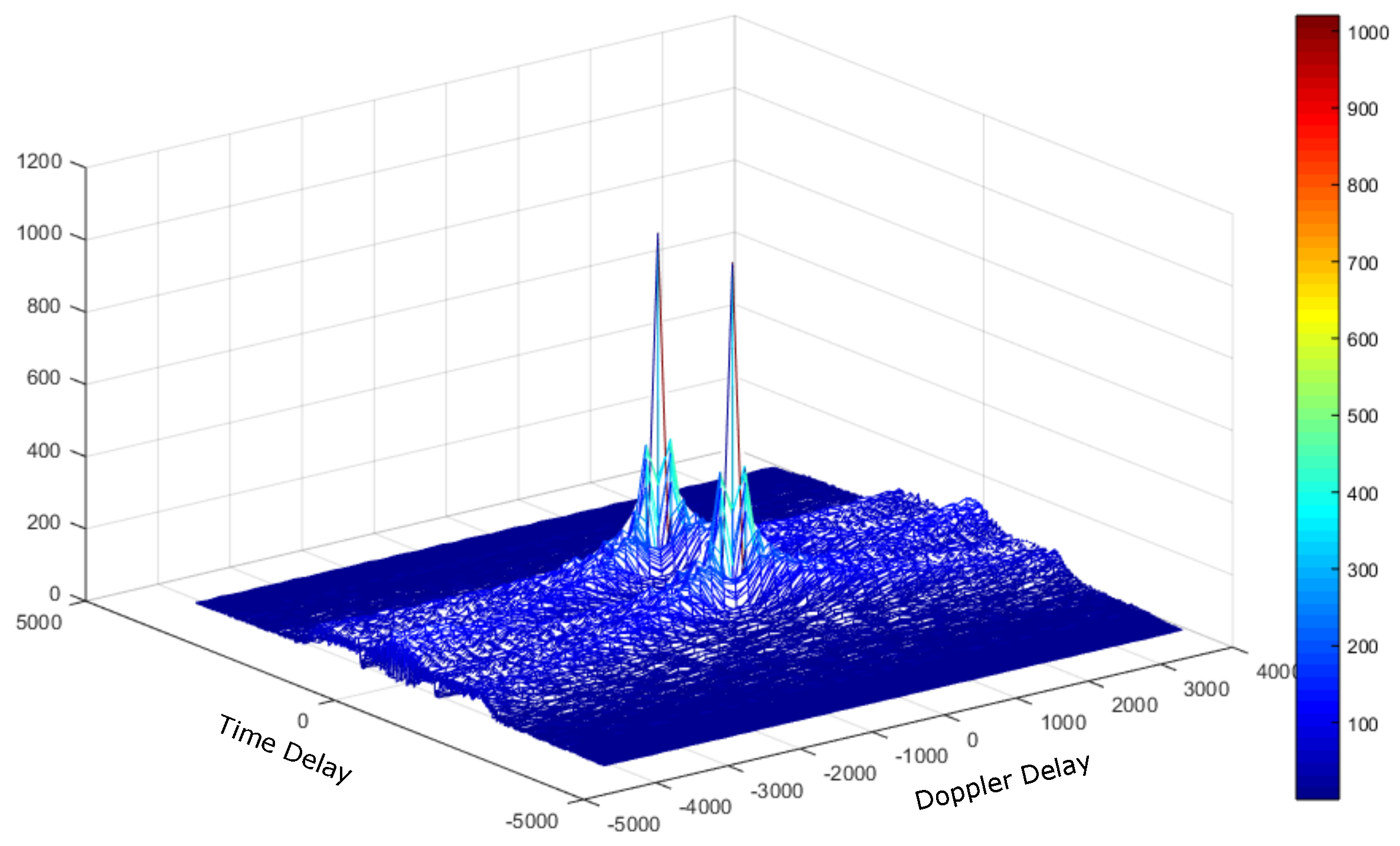
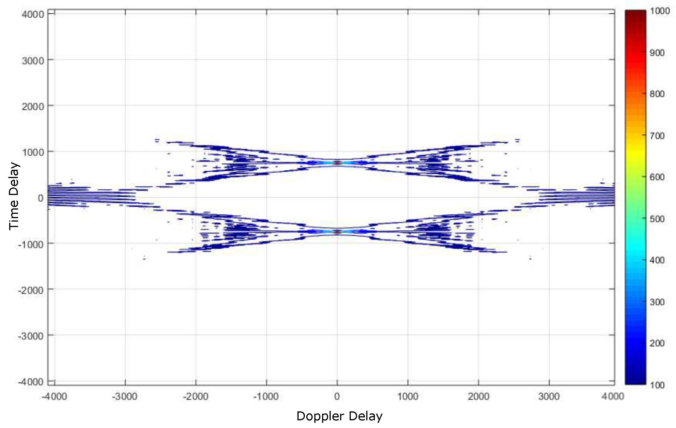
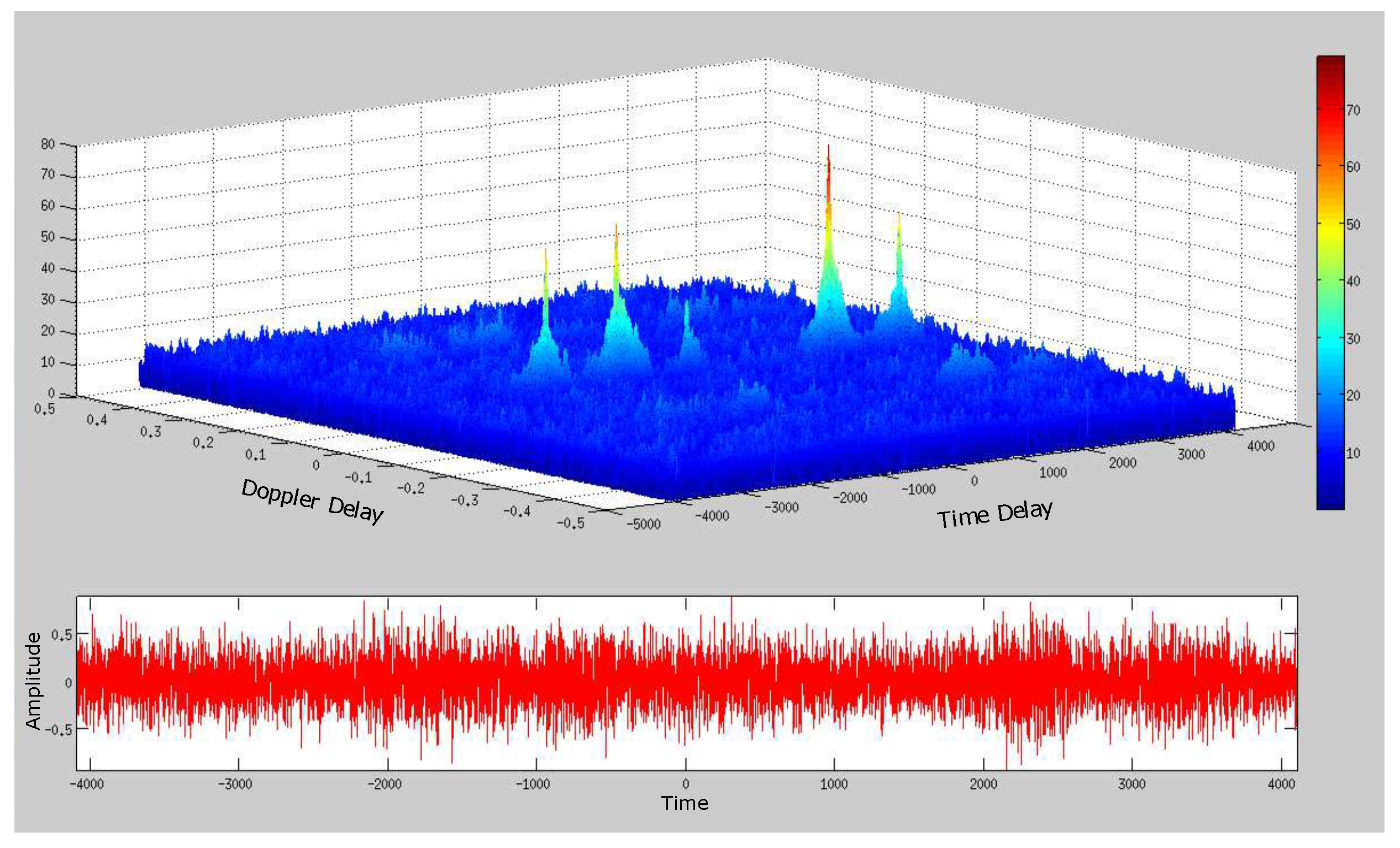
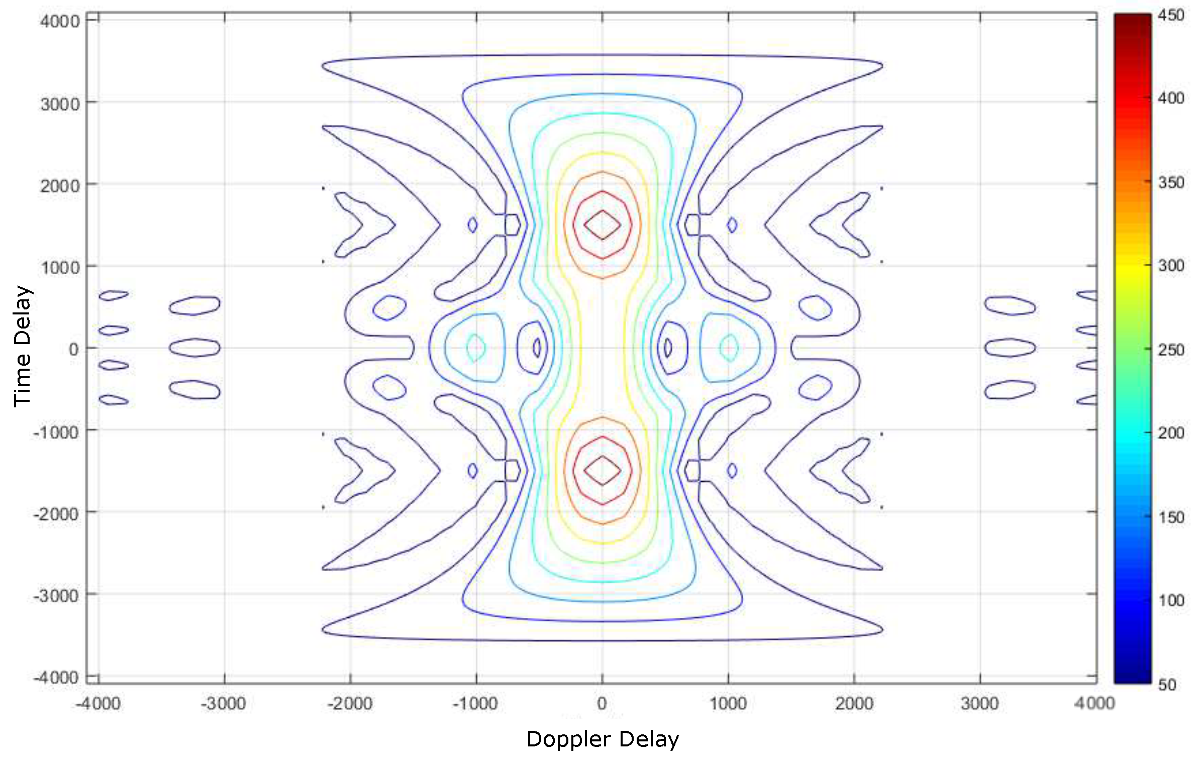
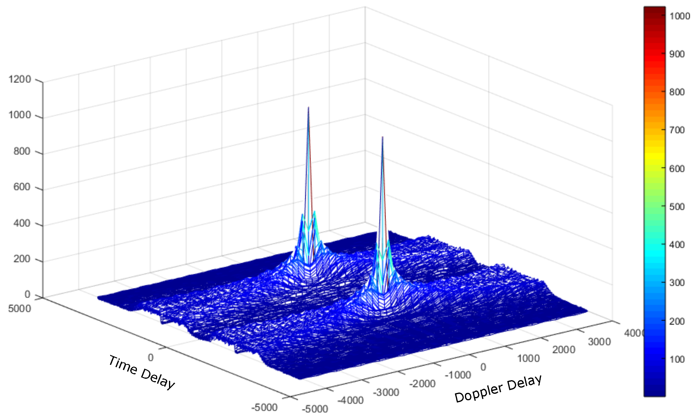
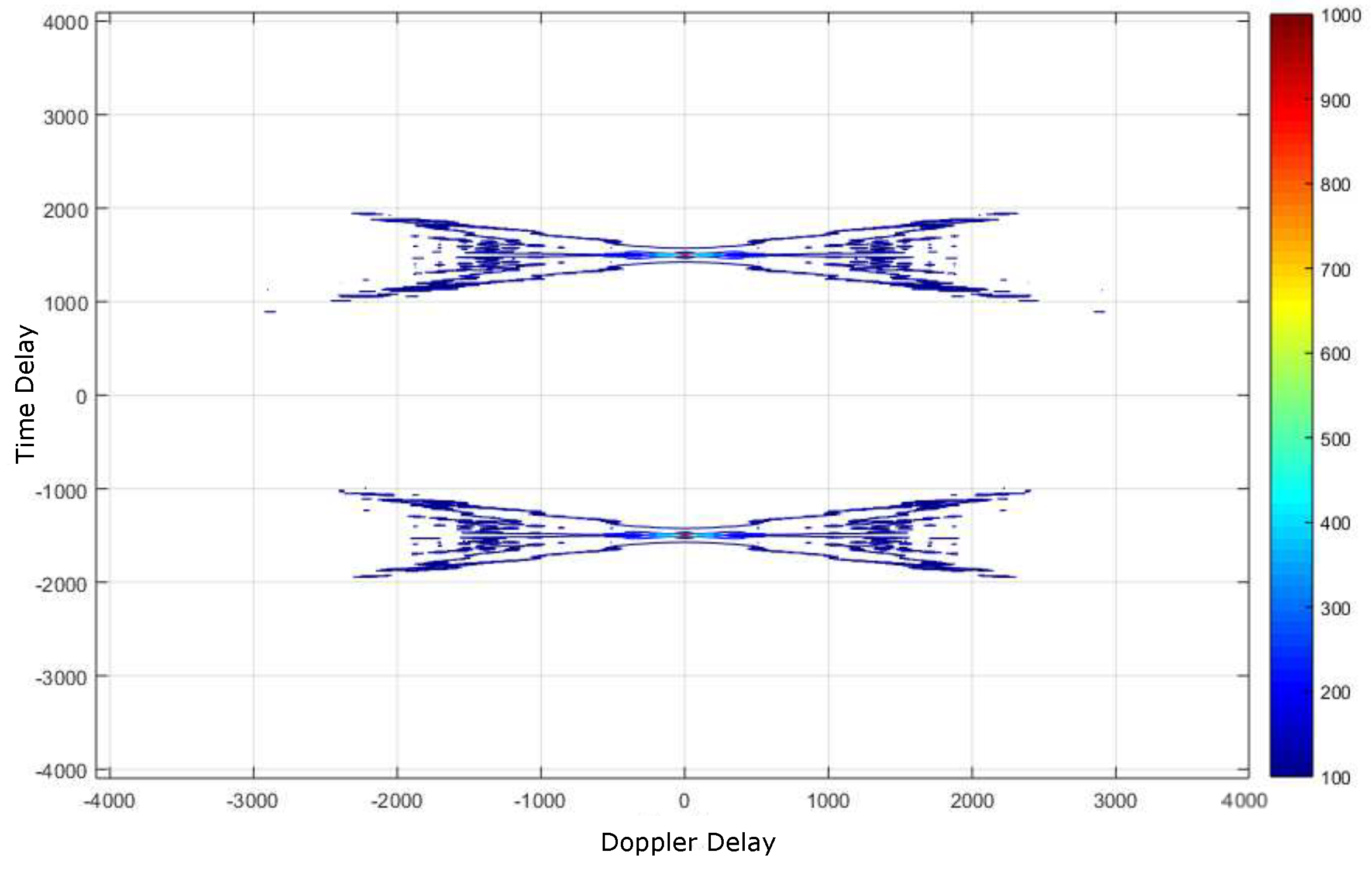
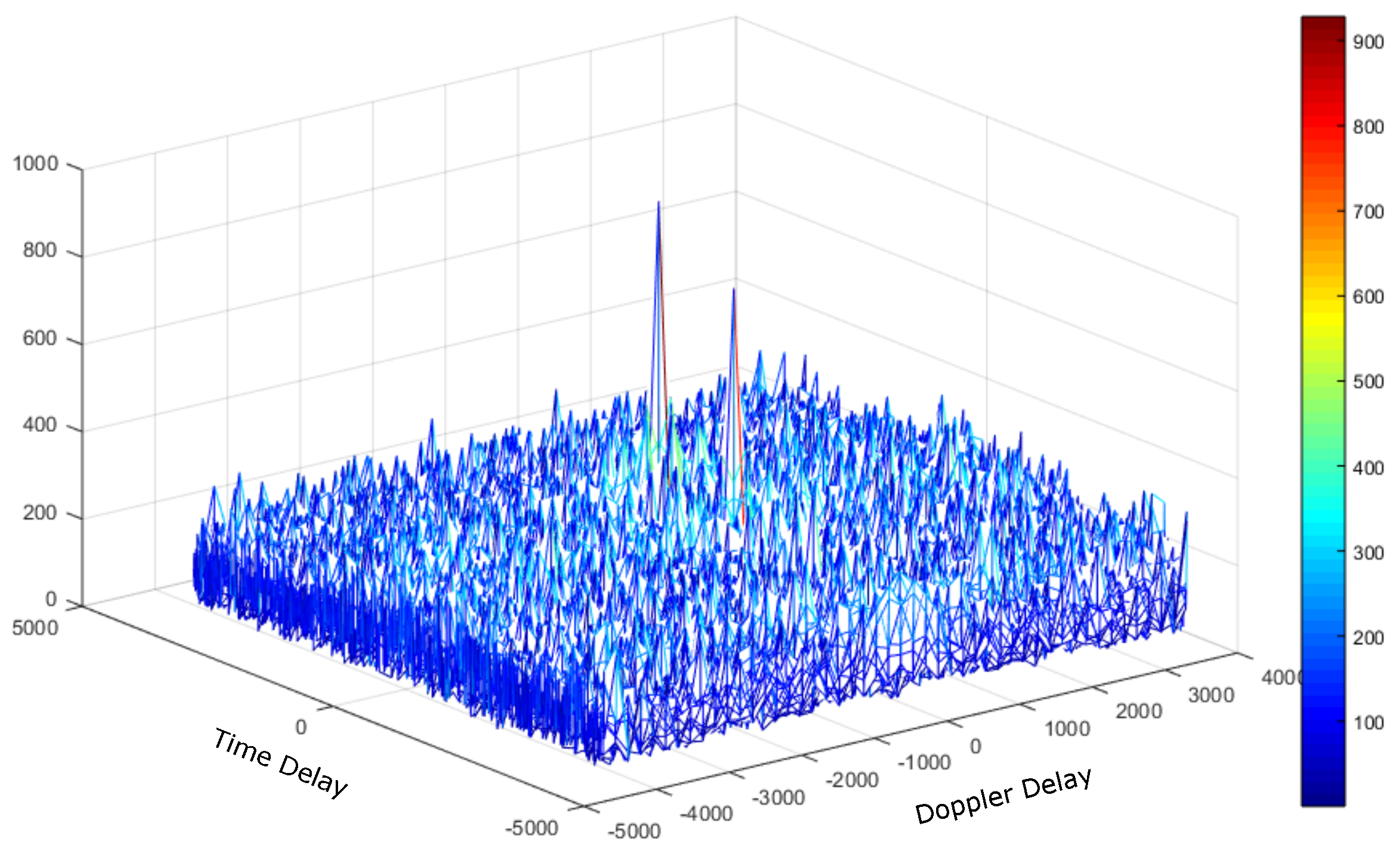
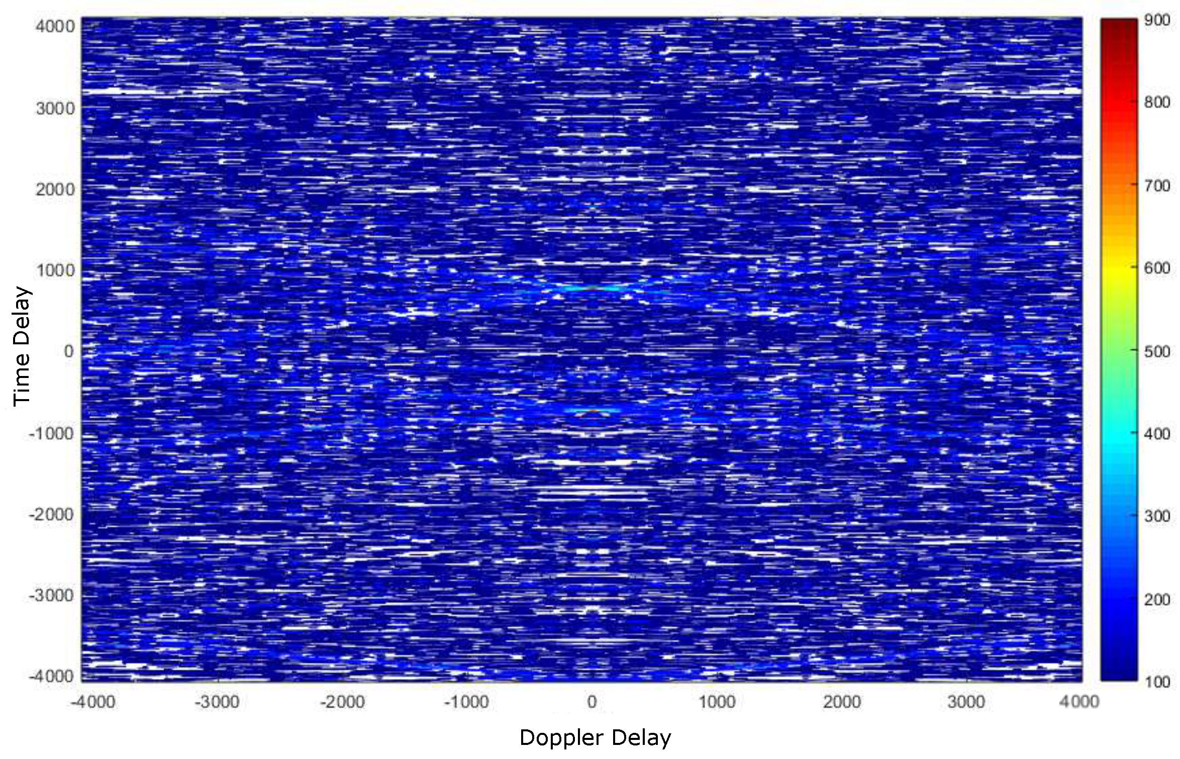
4.1. Deep Underwater Two-Object Tracking Example

The scattering interaction among the designed waveforms utilized at the transmitters was addressed using multidimensional, multi-component, polynomial phase (MMPP) signals and the processing of these signals using discrete Cohen distributions (DCDs) under a bidimensional harmonic analysis setting. In particular, the efficient computation of cross-ambiguity function operations was instrumental in solving the multiple objects scattering problem. Figure 10, Figure 11, Figure 12, Figure 13, Figure 14, Figure 15, Figure 16, Figure 17, Figure 18, Figure 19, Figure 20, Figure 21, Figure 22 and Figure 23 show the result of our bidimensional harmonic analysis algorithm applied to two nearby scatterers when these scatterers get closer. The bidimensional harmonic analysis was conducted using a diverse set of designed waveforms, including, sinusoidal, square and linear modulation or “chirp” pulses. The results showed, as expected, that the bidimensional harmonic analysis using chirp waveforms outperforms the analysis conducted using square waveform pulses.

The point target location accuracy of the SDET computational framework environment is addressed in this work on two fronts, i.e., the accuracy of the cross-ambiguity function of the transmitted and received pulses based on the design of the transmitted waveform and the accuracy of the relative position between the transmitter and receiver transducers in a MIMO configuration topology. To address the resolution issue through transmitter waveform generation for the cross ambiguity product, we followed the work of C. Y. Chen and P. P. Vaidyanathan on linear frequency modulation (LFM) chirp pulse time-bandwidth product design [28], as well as Brookner, E. work on MIMO array configuration design [29]. The relative position between transmitter and receiver transducers must be known to a sub-wavelength precision in order to improve a given point target location accuracy, and we followed the work of Pailhas, Y. and Petillot, Y. to accomplish this task [30].

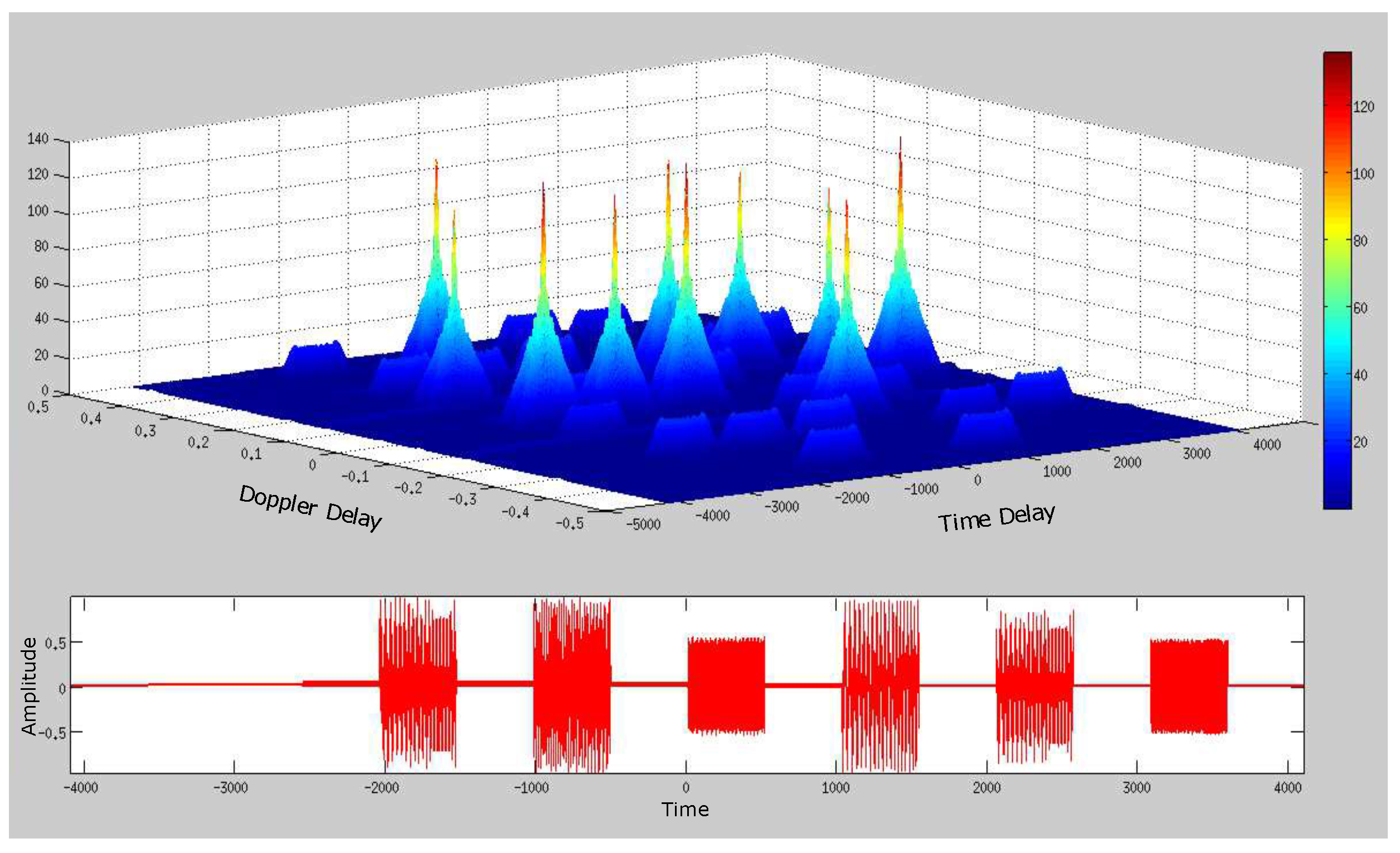
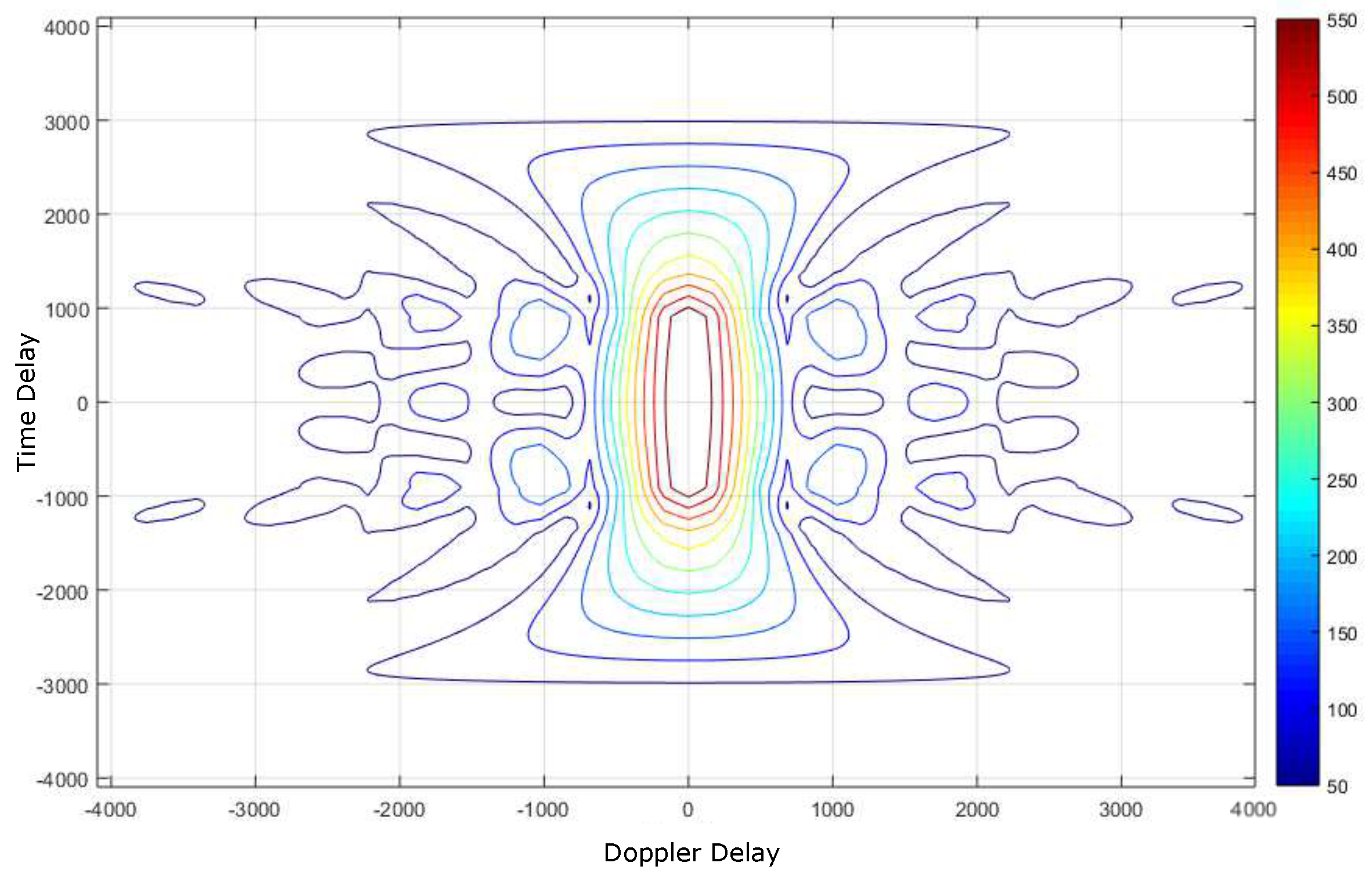
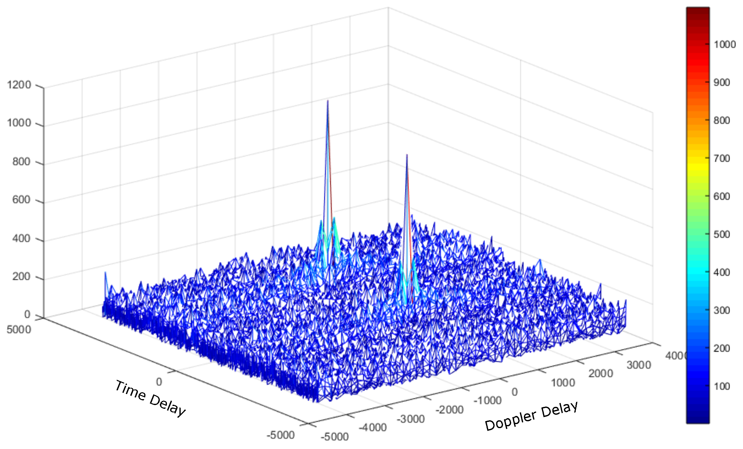
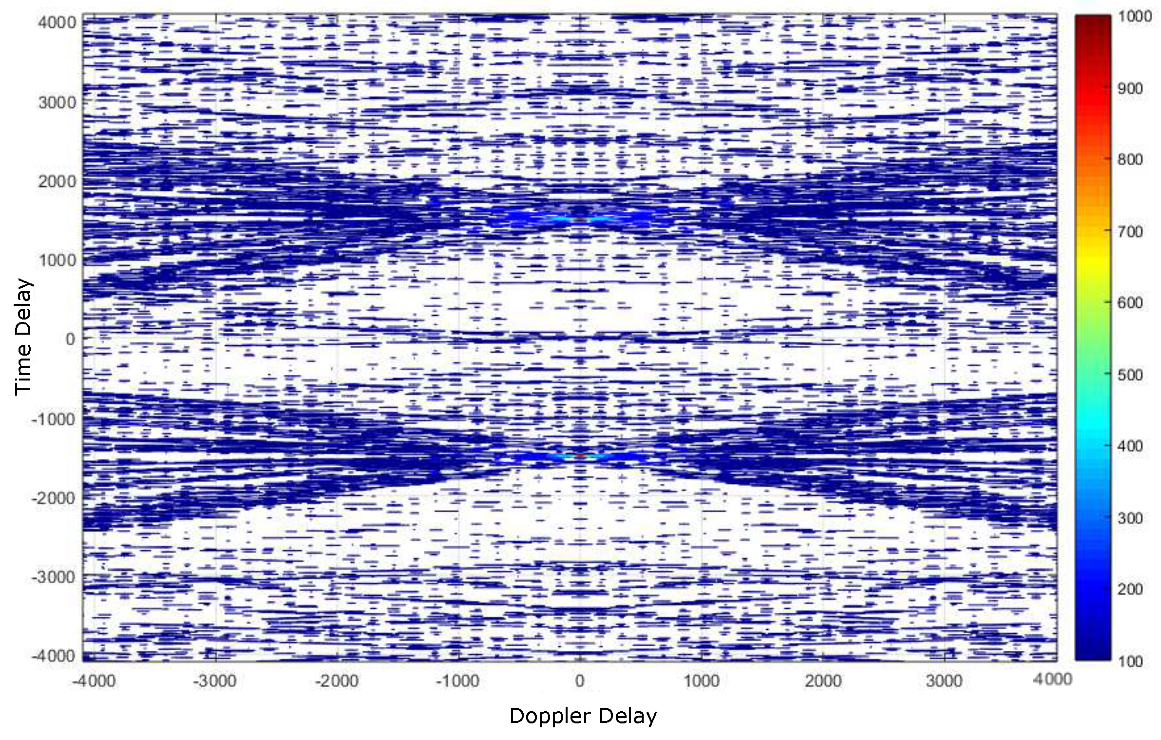
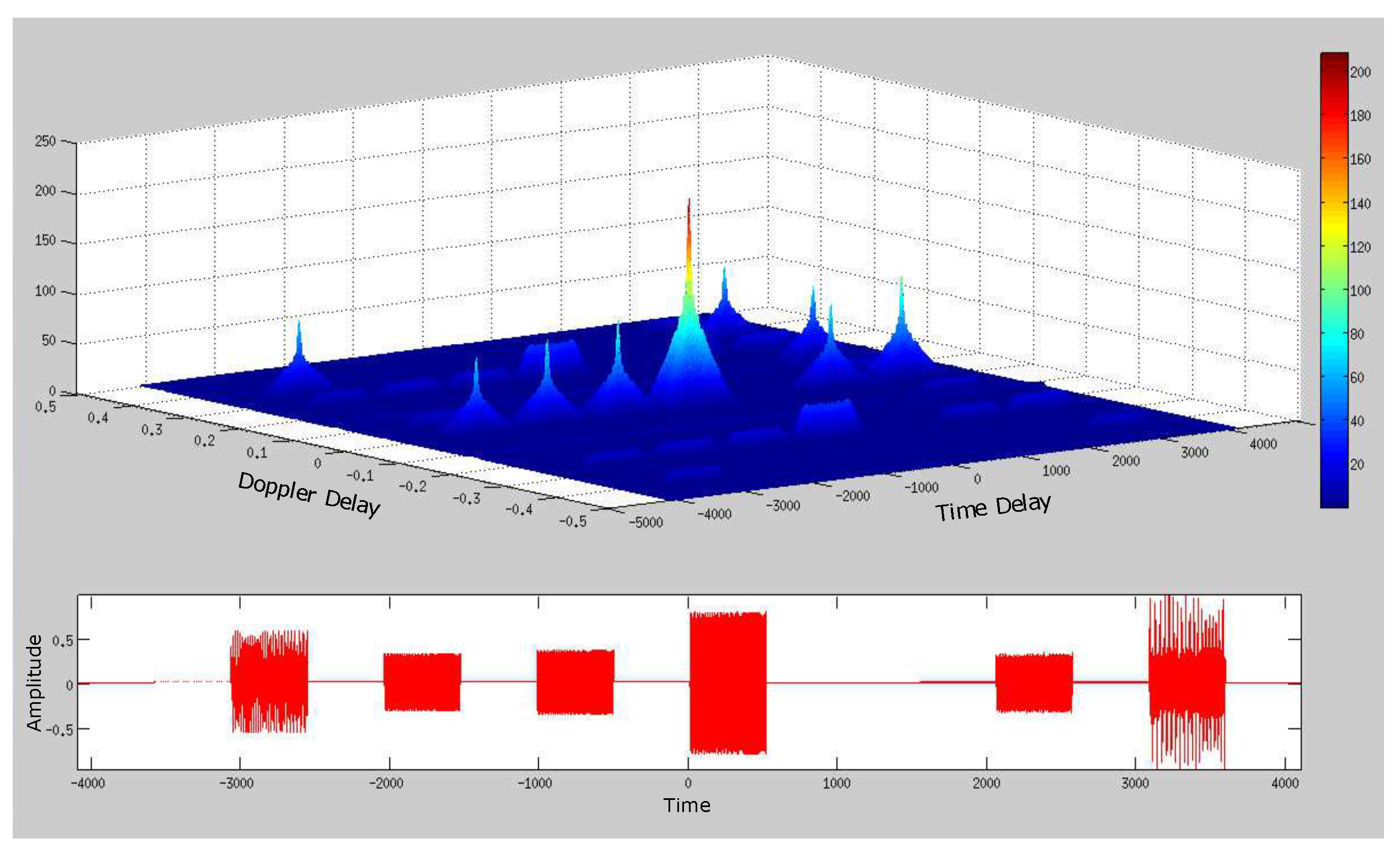
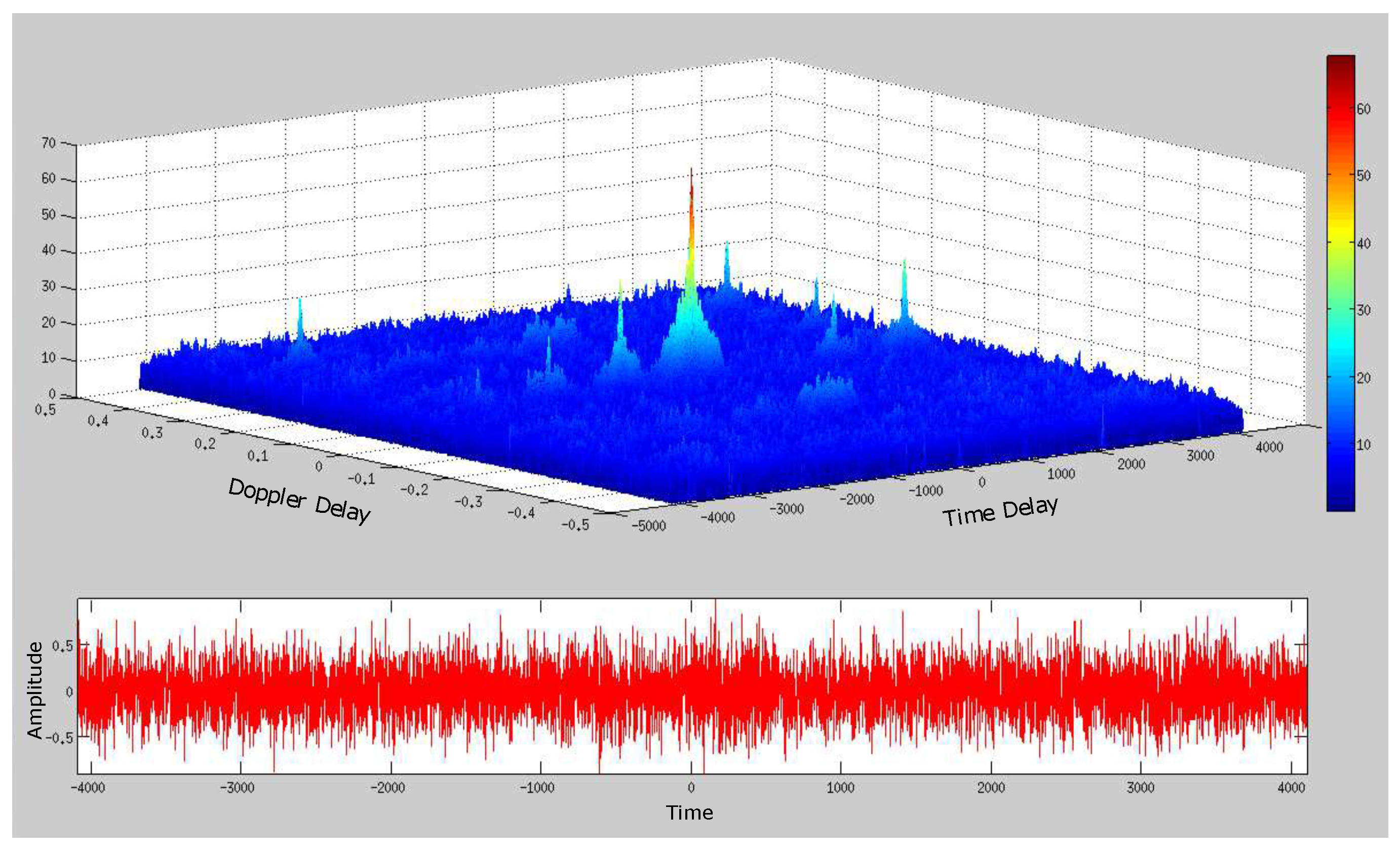
4.2. Deep Underwater Multiple Object Tracking Example

In this section, we describe a generalized testbed algorithm framework for simulating the tracking of multiple objects moving at a constant speed in a deep underwater environment. Figure 24 presents a tracking allocation chart when the number of tracked objects is equal to ten (10). However, the testbed algorithm framework was tested under multiple object tracking scenarios, each tracking scenario producing a different tracking allocation chart. Figure 25, Figure 26, Figure 27, Figure 28, Figure 29, Figure 30, Figure 31, Figure 32, Figure 33 and Figure 34 show the performance of the ten-object tracking simulation example. For simplicity, the chirp pulse waveforms were normalized in the amplitude and were also time normalized by setting the sampling time equal to unity.

5. Conclusions

This paper presented a computational framework for the analysis and design of signal processing algorithms utilized in the estimation of acoustic, doubly-dispersive, randomly time-variant, deep underwater communication channels. It introduced innovation along three main venues, i.e., using a mathematical language formulation to describe channel estimation processes, developing unique cyclic discrete time-frequency distributions for range Doppler estimation and exploiting the algebraic properties of block circulant structures to reduce the overall computational complexity. The results presented here are based on the work of Li, W. and Preisig, J.C. on the estimation of rapidly time-varying sparse channels, the work of Carrascosa, P.C. and Stojanovic, M. on underwater acoustic channel estimation using spatial multiplexing and the work of Yatawatta, S. and Petropulu, A. on blind channel estimation. Multiple object tracking operations were successfully accomplished using a $2\times 2$ MIMO channel estimation testbed structure.

The work presented in this paper demonstrated that the language of Kronecker products remains, after more than twenty (20) years, an invaluable tool for the formulation of signal processing algorithms. Kronecker products signal algebra, a branch of finite dimensional multilinear algebra, continues to produce fruitful results when dealing with the treatment of high dimensional signals. For example, we took advantage of the fact that the discrete Fourier transform (DFT) matrix may be represented as a product of sparse matrices, both using decimation in time (DIT) and decimation in frequency (DIF) to formulate cyclic filtering operations, using the property of the DFT matrix for the diagonalization of circulant matrices. This procedure allowed us to use the commutation theorem of Kronecker products in order to reduce the communication time between processors when dealing with large-scale block circulants. To the best of our knowledge, the parallel formulations of the matching pursuit algorithms presented in Kronecker products signal algebra language in this paper are new. These algorithm formulations were readily implemented using the pMatlab and PCT parallel programming environments. Through this parallel algorithm implementations, we demonstrated that the ORLSMP formulation was the most accurate; however, it was also the slowest.

References

1. Valera-Marquez, J. An Information-Based Complexity Approach to Acoustic Linear Stochastic Time-Variant Systems; ProQuest Dissertations and Theses; ProQuest: Ann Arbor, MI, USA, 2013. [Google Scholar]
2. Ray, S.; Lai, W.; Paschalidis, I.C. Statistical Location Detection with Sensor Networks. IEEE Trans. Inf. Theory 2006, 52, 2670–2683. [Google Scholar] [CrossRef]
3. Karoui, I.; Quidu, I.; Legris, M. Automatic Sea-Surface Obstacle Detection and Tracking in Forward-Looking Sonar Image Sequences. IEEE Trans. Geosci. Remote Sens. 2015, 53, 4661–4669. [Google Scholar] [CrossRef]
4. Kreucher, C.; Shapo, B. Multitarget Detection and Tracking Using Multisensor Passive Acoustic Data. IEEE J. Ocean. Eng. 2011, 36, 205–218. [Google Scholar] [CrossRef]
5. Daley, R.K.; Williams, A.; Green, M.; Barker, B.; Brodie, P. Can marine reserves conserve vulnerable sharks in the deep sea? A case study of Centrophorus zeehaani (Centrophoridae), examined with acoustic telemetry. Deep Sea Res. Part II Top. Stud. Oceanogr. 2015, 115, 127–136. [Google Scholar] [CrossRef]
6. Qi, C.; Wang, X.; Wu, L. Underwater acoustic channel estimation based on sparse recovery algorithms. IET Signal Process. 2011, 5, 739–747. [Google Scholar] [CrossRef]
7. Li, W.; Preisig, J. Estimation of Rapidly Time-Varying Sparse Channels. IEEE J. Ocean. Eng. 2007, 32, 927–939. [Google Scholar] [CrossRef]
8. Johnson, J.R.; Johnson, R.W.; Rodriguez, D.; Tolimieri, R. A Methodology for Designing, Modifying, and Implementing Fourier Transform Algorithms on Various Architectures. Circ. Syst. Signal Process. 1990, 9, 449–500. [Google Scholar] [CrossRef]
9. Carrascosa, P.C.; Stojanovic, M. Adaptive Channel Estimation and Data Detection for Underwater Acoustic MIMO-OFDM Systems. IEEE J. Ocean. Eng. 2010, 35, 635–646. [Google Scholar] [CrossRef]
10. Li, B.; Huang, J.; Zhou, S.; Ball, K.; Stojanovic, M.; Freitag, L.; Willett, P. MIMO-OFDM for High-Rate Underwater Acoustic Communications. IEEE J. Ocean. Eng. 2009, 34, 634–644. [Google Scholar]
11. Yatawatta, S.; Petropulu, A.P. Blind channel estimation in MIMO OFDM systems with multiuser interference. IEEE Trans. Signal Process. 2006, 54, 1054–1068. [Google Scholar] [CrossRef]
12. Van Loan, C. Computational Frameworks for the Fast Fourier Transform; Society for Industrial and Applied Mathematics: Philadelphia, PA, USA, 1992. [Google Scholar]
13. Franchetti, F.; Voronenko, Y.; Puschel, M. FFT Program Generation for Shared Memory: SMP and Multicore. In Proceedings of the 2006 ACM/IEEE Conference on Supercomputing, Tampa, FL, USA, 11–17 November 2006; p. 51.
14. Ali, A.; Johnsson, L.; Subhlok, J. Scheduling FFT Computation on SMP and Multicore Systems. In Proceedings of the 21st Annual International Conference on Supercomputing, Seattle, WA, USA, 17–21 June 2007; pp. 293–301.
15. Arce-Nazario, R.A.; Jiménez, M.; Rodríguez, D. Mapping of Discrete Cosine Transforms onto Distributed Hardware Architectures. J. Signal Process. Syst. 2008, 53, 367–382. [Google Scholar] [CrossRef]
16. Franchetti, F.; Puschel, M.; Voronenko, Y.; Chellappa, S.; Moura, J. Discrete Fourier Transform on Multicore. IEEE Signal Process. Mag. 2009, 26, 90–102. [Google Scholar] [CrossRef]
17. Kepner, J. Parallel Matlab for Multicore and Multinode Computers. Software, Environments, and Tools; Society for Industrial and Applied Mathematics (SIAM): Philadelphia, PA, USA, 2009; Volume 21. [Google Scholar]
18. Bello, P. Characterization of Randomly Time-Variant Linear Channels. IEEE Trans. Commun. Syst. 1963, 11, 360–393. [Google Scholar] [CrossRef]
19. Sandberg, J.; Hansson-Sandsten, M. Optimal Stochastic Discrete Time-Frequency Analysis in the Ambiguity and Time-Lag Domain. Signal Process. 2010, 90, 2203–2211. [Google Scholar] [CrossRef]
20. Amini, P.; Chen, R.R.; Farhang-Boroujeny, B. Filterbank Multicarrier Communications for Underwater Acoustic Channels. IEEE J. Ocean. Eng. 2015, 40, 115–130. [Google Scholar] [CrossRef]
21. Han, J.; Zhang, L.; Leus, G. Partial FFT Demodulation for MIMO-OFDM Over Time-Varying Underwater Acoustic Channels. IEEE Signal Process. Lett. 2016, 23, 282–286. [Google Scholar] [CrossRef]
22. Wang, W.Q. MIMO SAR OFDM Chirp Waveform Diversity Design With Random Matrix Modulation. IEEE Trans. Geosci. Remote Sens. 2015, 53, 1615–1625. [Google Scholar] [CrossRef]
23. Cheng, S.J.; Wang, W.Q.; Shao, H.Z. Spread Spectrum-Coded OFDM Chirp Waveform Diversity Design. IEEE Sens. J. 2015, 15, 5694–5700. [Google Scholar] [CrossRef]
24. He, X.; Song, R.; Zhu, W.P. Pilot Allocation for Distributed-Compressed-Sensing-Based Sparse Channel Estimation in MIMO-OFDM Systems. IEEE Trans. Veh. Technol. 2016, 65, 2990–3004. [Google Scholar] [CrossRef]
25. Duarte, M.F.; Baraniuk, R.G. Kronecker Compressive Sensing. IEEE Trans. Image Process. 2012, 21, 494–504. [Google Scholar] [CrossRef] [PubMed]
26. Lee, J.; Gil, G.T.; Lee, Y.H. Channel Estimation via Orthogonal Matching Pursuit for Hybrid MIMO Systems in Millimeter Wave Communications. IEEE Trans. Commun. 2016, 64, 2370–2386. [Google Scholar] [CrossRef]
27. Kuck, D.J. High Performance Computing: Challenges for Future Systems; Oxford University Press, Inc.: New York, NY, USA, 1996. [Google Scholar]
28. Chen, C.Y.; Vaidyanathan, P.P. MIMO Radar Ambiguity Properties and Optimization Using Frequency-Hopping Waveforms. IEEE Trans. Signal Process. 2008, 56, 5926–5936. [Google Scholar] [CrossRef]
29. Brookner, E. MIMO radars and their conventional equivalents. In Proceedings of the 2015 IEEE Radar Conference (RadarCon), Arlington, VA, USA, 10–15 May 2015; pp. 7–15.
30. Pailhas, Y.; Petillot, Y. MIMO sonar systems for harbour surveillance. In Proceedings of the OCEANS 2015, Genova, Italy, 18–21 May 2015; pp. 1–6.
Figure 1. Deep underwater multiple object tracking scenario.
Jsan 06 00002 g001
Figure 2. Deep underwater time-frequency dispersive channel model.
Jsan 06 00002 g002
Figure 3. SISO input/output channel configuration.
Jsan 06 00002 g003
Figure 4. MISO input/output channel configuration.
Jsan 06 00002 g004
Figure 5. SIMO input/output channel configuration.
Jsan 06 00002 g005
Figure 6. Kuck’s diagram for the parallel MIMO acoustic, linear, stochastic (ALS) estimation problem.
Jsan 06 00002 g006
Figure 7. MIMO channel estimation testbed structure.
Jsan 06 00002 g007
Figure 8. MIMO ( 2 × 2 ). Delay-Doppler spread function U 1 , 0 .
Jsan 06 00002 g008
Figure 9. MIMO ( 2 × 2 ). Delay-Doppler spread function U 1 , 1 .
Jsan 06 00002 g009
Figure 10. Two nearby scatterers using square pulses, with no noise.
Jsan 06 00002 g010
Figure 11. Two nearby scatterers using square pulses: 2D, with no noise.
Jsan 06 00002 g011
Figure 12. Two nearby scatterers using square pulses, at −5 dB SNR.
Jsan 06 00002 g012
Figure 13. Two nearby scatterers using square pulses, at −5 dB SNR.
Jsan 06 00002 g013
Figure 14. Two closer scatterers using square pulses, with no noise.
Jsan 06 00002 g014
Figure 15. Two closer scatterers using square pulses: 2D, with no noise.
Jsan 06 00002 g015
Figure 16. Two nearby scatterers using chirp pulses (multidimensional, multi-component, polynomial phase (MMPP)) with no noise.
Jsan 06 00002 g016
Figure 17. Two nearby scatterers using chirp pulses (MMPP): -2D, with no noise.
Jsan 06 00002 g017
Figure 18. Two nearby scatterers using chirp pulses (MMPP), at −5 dB SNR.
Jsan 06 00002 g018
Figure 19. Two nearby scatterers using chirp pulses (MMPP): 2D, at −5 dB SNR.
Jsan 06 00002 g019
Figure 20. Two closer scatterers using chirp pulses (MMPP), with no noise.
Jsan 06 00002 g020
Figure 21. Two closer scatterers using chirp pulses (MMPP): 2D, with no noise.
Jsan 06 00002 g021
Figure 22. Two closer scatterers using chirp pulses (MMPP), at −5 dB SNR.
Jsan 06 00002 g022
Figure 23. Two closer scatterers using chirp pulses (MMPP): 2D, at −5 dB SNR.
Jsan 06 00002 g023
Figure 24. Multiple object tracking (MOT) allocation chart with scattering points P l , l Z L .
Jsan 06 00002 g024
Figure 25. Multiple object tracking using MMPP “chirp pulses”, at Tracking Time 1, with no noise.
Jsan 06 00002 g025
Figure 26. Multiple object tracking using MMPP “chirp pulses”, at Tracking Time 1, with −5 dB SNR.
Jsan 06 00002 g026
Figure 27. Multiple object tracking using MMPP “chirp pulses”, at Tracking Time 2, with no noise.
Jsan 06 00002 g027
Figure 28. Multiple object tracking using MMPP “chirp pulses”, at Tracking Time 2, with −5 dB SNR.
Jsan 06 00002 g028
Figure 29. Multiple object tracking using MMPP “chirp pulses”, at Tracking Time 3, with no noise.
Jsan 06 00002 g029
Figure 30. Multiple object tracking using MMPP “chirp pulses”, at Tracking Time 3, with −5 dB SNR.
Jsan 06 00002 g030
Figure 31. Multiple object tracking using MMPP “chirp pulses”, at Tracking Time 4, with no noise.
Jsan 06 00002 g031
Figure 32. Multiple object tracking using MMPP “chirp pulses”, at Tracking Time 4, with −5 dB SNR.
Jsan 06 00002 g032
Figure 33. Multiple object tracking using MMPP “chirp pulses”, at Tracking Time 5, with no noise.
Jsan 06 00002 g033
Figure 34. Multiple object tracking using MMPP “chirp pulses”, at Tracking Time 5, with −5 dB SNR.
Jsan 06 00002 g034