Estimating the Lifetime of Wireless Sensor Network Nodes through the Use of Embedded Analytical Battery Models

Abstract

The operation of Wireless Sensor Networks (WSNs) is subject to multiple constraints, among which one of the most critical is available energy. Sensor nodes are typically powered by electrochemical batteries. The stored energy in battery devices is easily influenced by the operating temperature and the discharge current values. Therefore, it becomes difficult to estimate their voltage/charge behavior over time, which are relevant variables for the implementation of energy-aware policies. Nowadays, there are hardware and/or software approaches that can provide information about the battery operating conditions. However, this type of hardware-based approach increases the battery production cost, which may impair its use for sensor node implementations. The objective of this work is to propose a software-based approach to estimate both the state of charge and the voltage of batteries in WSN nodes based on the use of a temperature-dependent analytical battery model. The achieved results demonstrate the feasibility of using embedded analytical battery models to estimate the lifetime of batteries, without affecting the tasks performed by the WSN nodes.

1. Introduction

Wireless Sensor Networks (WSNs) are typically employed to support sensing/actuating activities in different application domains (e.g., industrial, commercial and residential) mainly due to their flexibility, low cost and low implementation complexity. A well-known constraint for the deployment of WSNs is the lifetime of their sensor nodes, which is upper-bounded due to stored energy limitations. The main limitation is the reduced battery capacity, which upper-bounds the operating life of the sensor node. In this context, it would be important to estimate both the battery State of Charge (SoC) and its lifetime according to the set of tasks executed by the nodes (e.g., data reception/transmission/processing tasks). For instance, this type of information is highly relevant, whenever energy-aware algorithms have to be implemented in the sensor nodes. However, estimating the battery lifetime in WSN nodes is a difficult task, as several factors influence their operation (e.g., chemical composition of the battery itself, operating temperature and discharge current) [1], resulting in a non-linear behavior over time [2,3,4].

There are two major options to estimate the battery operating behavior [5]: (i) hardware-based solutions, which involve the use of Integrated Circuits (ICs) that provide the relevant battery data; and (ii) software-based solutions, that usually require the use of adequate mathematical models. These two options are discussed below.

Smart batteries use ICs along with the electrochemical cell(s) to provide relevant data about the battery behavior (e.g., voltage, temperature, current) [6] and, in some cases, estimations about its operating behavior (e.g., SoC and remaining lifetime [7]) to the connected device (e.g., laptops, smartphones, cameras) [8,9]. However, the use of these hardware-based approaches increases the cost of producing batteries by approximately 25% (fuel gauge ICs costs about $2–3) [10]. In the context of WSNs, where the deployment of a large number of nodes may be required, such a solution may become economically infeasible. In addition, hardware-based solutions involving the use of ICs are often adapted to the integrated battery technology, where lookup tables are used to reconstruct the characteristics of the used cell(s) under different operating conditions [11]. Thus, it would be relevant to adopt software-based solutions able to accurately estimate the battery behavior of WSN nodes, without requiring the use of dedicated hardware. An important requirement is that, whatever the estimation approach, it must (i) be flexible enough to support different battery technologies; and (ii) present low computational cost due to the hardware constraints of sensor nodes.

Analytical battery models typically rely on a set of differential equations to estimate the battery behavior. Usually, these models are implemented in WSN simulators to estimate the operating behavior of the sensor nodes before their actual deployment. Within this context, the current battery condition is mathematically estimated to enable the deployment of energy-aware algorithms and protocols [12,13,14]. However, it is necessary to evaluate whether it is possible (or not) to implement similar differential equations-based models in real-world WSN nodes. It would be also necessary to assess the impact of implementing such mathematical models upon COTS low-power hardware. A pertinent question in this scenario is how does the computation of battery models may affect the lifetime of WSN nodes, which are usually based on low-power micro-controllers to save energy? In other words, and regarding the computational cost, is it feasible to perform a battery model computation upon a sensor node, in order to implement an on-line SoC determination and the related voltage level tracking functions?

The main target of this paper is to assess the usability of a low complexity analytical battery model [15], the Temperature-Dependent Kinetic Battery Model (T-KiBaM) [16], implemented upon Micro-Controller Units (MCUs) with low computational power, such as the ATmega328P and ATmega128RFA1 [17]. These MCUs are similar to those found in low-power COTS WSN nodes, e.g., the MICAz, which is based on the ATmega128L. Both ATmega-328P/-128RFA1 MCUs are widely available as the processing units of low cost WSN nodes. The main contributions of this work are:

• The experimental evaluation of a computationally inexpensive method to on-line estimate both the lifetime and State of Charge of batteries in real-world COTS WSN nodes with low computational capacity, small built-in memory and energy consumption constraints.
• A report on the implementation of light and accurate analytical battery models upon multiple low-power MCUs, typically used in real-world COTS WSN nodes.
• The implementation of a proof-of-concept application example demonstrating the usability of the T-KiBaM analytical model [16] to estimate the battery SoC and to on-line track its voltage level during the node activity period, as long as the discharge profile of the battery is known.

Next sections of this paper are organized as follows. Section 2 presents the related work. Section 3 introduces the basics about the T-KiBaM model, which includes the dependence of temperature on the estimation of the SoC of the battery, as well as a more accurate battery voltage model called Temperature-Dependent Voltage Model (TVM). Section 4 discusses the details about the experimental assessments and also about the model implementation. Section 5 presents the achieved results when running T-KiBaM upon low-power MCUs. Section 6 extends the previous section by adding a proof-of-concept application example, where other metrics are evaluated in an emulated operating scenario. Finally, Section 7 concludes the paper and presents future work.

2. Related Work

This section addresses the state-of-the-art in different areas of research related to this work. There are several studies dealing with the problem of estimating the SoC in batteries for different types of applications (e.g., electric vehicles) [18,19,20,21]. Nevertheless, the applicability of the reported results within the WSN context is difficult, as both the battery capacities and discharge profiles considered in these works are very different from those found in sensor nodes. Therefore, this section is divided in the two following items: (i) assessment of the computational cost of executing complex algorithms in micro-controllers with low computing capacity and (ii) deployment of analytical battery models in WSN nodes. Discussions on these topics are presented below.

There are several available studies in the literature evaluating the computational cost of running complex algorithms in low-power MCUs. For instance, Çakiroğlu [22] evaluated block cypher algorithms running upon an 8-bit Atmel ATmega128 MCU. The study assessed the execution of complex algorithms regarding the code/data memory requirements, execution time and throughput. Within the WSN context, Wei et al. [23] evaluated the overhead of cryptography algorithms suitable for WSNs. The authors evaluated the following metrics: clock cycles, code size, SRAM usage, and power consumption. The results showed that some algorithms are more appropriate when considering time-critical or energy-efficient applications, while others are more appropriate as they consume less SRAM memory. Capo-Chichi et al. [24] evaluated and compared the execution of data compression algorithms when using an ultra low-power micro-controller, known as MSP430, from Texas Instruments. The study aimed to evaluate the trade-off between energy consumption and compression efficiency. Guo et al. [25] presented two optimization approaches (Gauss-Newton Algorithm and Particle Swarm Optimization) to improve the localization of nodes in WSNs. The authors experimentally evaluated issues such as execution time, the number of iterations, memory usage and quality of estimation of the localization. Othman et al. [26] studied the cost of providing security in WSNs by implementing three cryptographic algorithms (AES, RC5 and RC6) upon MICA2 nodes. The authors analyzed memory consumption, operation time and energy consumption when using each one of the algorithms. Quirino et al. [27] presented the performance assessment of asymmetric cryptographic algorithms within the WSN context. Authors use three different platforms (ARM, MSP430 and AVR ATmega128) to evaluate the processing time of the algorithms. Pardo et al. [28] implemented an Artificial Neural Network (ANN) algorithm upon a low-cost chip (CC1110F32) for the purpose of developing autonomous intelligent WSNs to monitor and forecast the indoor temperature in smart homes. The authors were concerned with memory consumption and the use of computational resources, with the main objective of evaluating the feasibility of the implementation. Panić et al. [29] presented a micro-controller specifically designed to support WSN applications with severe security demands. The authors tested the developed chip with known cryptographic algorithms (ECC, AES and SHA-1), observing the execution time, security level and power consumption. Among all previously mentioned papers, note that the main evaluated metrics are: execution time, memory usage and power consumption. Some papers also evaluate other specific metrics related to the assessed algorithms, such as number of iterations and quality of the obtained results.

Regarding the implementation of analytical battery models upon WSN sensor nodes, Leveque et al. [30] presented a modeling approach to simulate the behavior of heterogeneous systems composed of WSN nodes. First, the authors model a set of WSN nodes for monitoring seismic perturbations, using a 32-bit microprocessor to solve a system of mathematical non-linear equations, that predict the battery behavior. This study case was implemented in SystemC-AMS, an extension of SystemC that models Analog/Mixed Systems. A computer simulates the system based on a 100-MHz microcontroller. In fact, this was a simulation-based assessment, with no hardware implementation. Other works also evaluated ways to estimate the battery lifetime on WSN nodes through simulations [6,31,32] or emulation [33]. Rahmé et al. [34] adapted the Rakhmatov and Vrudhula [35] analytical battery model to estimate the remaining energy in batteries of WSN nodes. The proposed battery model reduces the computational complexity and requires low memory usage. However, the achieved results illustrate relatively high errors (8–14%), when compared to the experimentally assessed results. Kerasiotis et al. [36] addressed the problem of estimating the battery lifetime on a WSN platform known as TelosB. In this case, the proposed methodology uses the energy consumption of each module to model the battery behavior of the node. The work used average load values to characterize the main operations performed at the node. The results indicated errors between 2–3% in comparison with experimental data for different duty cycles. Nataf and Festor [37] implemented the Rakhmatov and Vrudhula model in a dedicated operating system for WSN nodes known as Contiki. Tests included evaluations of node bootstrap and networking processes. In addition, the paper evaluated the accuracy of the lifetime estimate for different MAC protocols, also implemented in the Contiki operating system. Rukpakavong et al. [38] proposed a dynamic approach that considers several factors which can influence the battery lifetime, such as self-discharge, aging, discharge current and temperature. This approach was implemented in two WSN platforms: MICA2 and N740 NanoSensor. The results indicated deviations from −3.5% to 2.5% when estimating the battery lifetime. However, it was assumed that the voltage value must be read at the beginning of the calculations to evaluate the initial battery capacity, i.e., this approach did not track the voltage of the battery over time. In addition, the work did not consider the recovery effect, which is an important effect in scenarios where the WSN nodes operate in duty cycle scheme.

The main advantage of the methodology proposed in this paper is related to the deployment of a temperature-dependent battery model, which can be used to predict the behavior of the battery in low-power WSN nodes regardless of the associated hardware. The proposed methodology assumes that there is a cyclical operation pattern for the WSN nodes (e.g., a duty cycle), so that the discharge profile can be used as input parameter to compute the battery behavior over time (open-loop computation). Figure 1 depicts an example of a discharge profile based on a MICA2DOT WSN node [39]. By using this type of discharge profiles, it becomes possible to obtain two information about the battery: (i) the SoC, which is obtained through the analytical battery model proposed in Section 3.2; and (ii) the voltage level, which is concurrently obtained through the execution of the voltage model presented in Section 3.2.1.

3. Background

This section presents the main concepts involved in this paper. Briefly, the original Kinetic Battery Model (KiBaM) [40,41] model is presented along with its voltage model. Next, it is introduced a summary on the Temperature-Dependent Kinetic Battery Model (T-KiBaM) [16], an extension of the KiBaM model that includes the effect of temperature on the predictions about both the lifetime and voltage of the battery.

3.1. Kinetic Battery Model (KiBaM)

KiBaM is one of the first high-accuracy analytical battery models that was proposed in the early nineties. It is based on an intuitive approach to model the behavior of high-capacity Lead-Acid batteries over time. This model uses a two-tank analogy to describe the battery charge and discharge processes, as shown in Figure 2.

In this model, the available charge tank is the power supply for any device that consumes a current over time, $I\left(t\right)$. The average value of current I is considered for each period of time t. The bound charge tank holds part of the battery charge, which can be transposed to the available charge tank at a rate $k^{\prime }$ through a valve that interconnects both thanks. In this context, $k^{\prime }$ is a constant that represents the rate of a chemical diffusion/reaction process. The transfer of charge occurs as long as there is a height difference between the charges of both tanks, i.e., $\delta =h_2-h_1\ne 0$. The constant c indicates the total charge ratio stored in the available charge tank. The battery remains operational as long as there is charge in the available charge tank (i.e., SoC $>0$%), regardless of whether there is charge in the bound charge tank or not. A system of differential equations is able to describe the KiBaM model (refer to [40] for further details). Laplace transforms are able to solve such a system of differential equations, resulting in:

$$\left\{\begin{array}{c}{\displaystyle q_1=q_{1,0}·e^{-k·t}+\frac{(q_0·k·c-I)·(1-e^{-k·t})}{k}-\frac{I·c·(k·t-1+e^{-k·t})}{k}}\hfill \\ {\displaystyle q_2=q_{2,0}·e^{-k·t}+q_0·(1-c)·(1-e^{-k·t})-\frac{I·(1-c)·(k·t-1+e^{-k·t})}{k},}\hfill \end{array}\right.$$

(1)

where $q_{1,0}$ and $q_{2,0}$ are the amount of charge in the available and bound charge tanks, respectively, when $t=0$. A new rate constant is defined as $k=k^{\prime }/(c·(1-c))$. In addition, $q_0=q_{1,0}+q_{2,0}$, where $q_0$ is the amount of charge in the battery at $t=0$. Thus, the constants required for the use of KiBaM are: $q_{max}$ (the maximum capacity of the battery), c (a fraction of the capacity stored in the available charge tank) and k (the rate constant). Such constants can be obtained from discharge tests with real batteries, as presented in [40], or applying the data-sheet values when available, and used in analytical evaluations to determine the SoC of the battery.

The SoC of the battery can be calculated from the relation of the unavailable charge of the battery, $q_{un}\left(t\right)=(1-c)·\delta \left(t\right)$, and also from Equation (1) along with the discharge current, $i\left(t\right)$, as follows [4]:

$${\displaystyle SOC\left(t\right)={SOC}_{initial}-\frac{1}{q_{max}}\left[\int i\left(t\right)dt+q_{un}\left(t\right)\right].}$$

(2)

3.1.1. KiBaM Voltage Model

The earlier KiBaM model is also able to track the battery voltage (V) over time. To do so, it becomes necessary to expand the battery model with the related electrical model:

$$V=E-I·R_0,$$

(3)

where $R_0$ is the internal resistance of the battery and E is the internal voltage of the battery. For discharge purposes, E can be obtained using the following equation:

$$E=E_{min}+(E_{0,d}-E_{min})\frac{q_1}{q_{1,max}},$$

(4)

where $E_{min}$ is the minimum allowed internal discharge voltage (“empty”), $E_{0,d}$ is the maximum internal discharge voltage (“full”) and $q_{1,max}$ is the maximum capacity of the available charge tank (obtained from $q_{max}$). The internal resistance, $R_0$, can be experimentally determined using constant discharge currents. Its value is represented by the slope $dV/dI$, when the battery is fully charged. In other words, the slope of $V\times I$ gives the value for $R_0$ [40].

Note that this voltage model is quite limited for the most commonly used battery technologies within the WSN context (e.g., Ni-MH or Li-ion), as it assumes a linear behavior when the battery is discharged with a constant current. A more accurate solution will be presented in the next section.

3.2. Temperature-Dependent Kinetic Battery Model (T-KiBaM)

T-KiBaM [16] is an extension of the KiBaM model that aggregates the effects caused by the use of the battery at different temperatures, which may change both its lifetime and its voltage behavior over time. Briefly, the thermal effect can accelerate the rate of reactions inside the battery, implying that the battery can provide a higher effective capacity at high temperatures [42]. The influence of temperature on the rate of a chemical reaction follows an empirical law known as the Arrhenius equation:

$$k=A·e^{-\frac{E_a}{R·T_k}},$$

(5)

where k is the constant rate of a reaction, A is the pre-exponential factor or pre-factor (in s${}^{-1}$), $E_a$ is the activation energy (in KJ/mol), R is the universal gas constant (8.314 × 10${}^{-3}$ KJ/mol·K) and $T_k$ is the temperature (in Kelvin). Considering that both k parameters from KiBaM and the Arrhenius equation refer to a constant reaction rate, it becomes possible to establish the following relationship: $k_{\mathrm{KiBaM}}=k_{\mathrm{Arrhenius}}$. Therefore:

$$k_{\mathrm{KiBaM}}=A·e^{-\frac{E_a}{R·T_k}}.$$

(6)

That is, the parameter k of the KiBaM model now follows the Arrhenius relation, and may vary according to the operating temperature of the battery. As described by Rodrigues et al. [16], a reduced number of experimental measurements is required to determine the values of constants A and $E_a$.

In addition, temperature also influences the charge capacity provided by the battery. Typically, batteries provide higher effective capacities at higher temperatures [42] and lower effective capacities when used at lower temperatures [43]. Within this context, it is crucial to adjust T-KiBaM to the technology of the battery being modeled (e.g., Ni-MH or Li-ion). Briefly, it is necessary to experimentally observe the behavior of the battery at different temperatures and discharge currents. Then, it is possible to establish a Correction Factor (CF), which allows the creation of a function capable of correcting the initial capacity of the battery according to the temperature in Celsius degrees ($T_c$). Please refer to [16] for details on how to find a function that allows calculating the CF value.

3.2.1. T-KiBaM Voltage Model

T-KiBaM also includes its own Temperature-Dependent Voltage Model (TVM) [16], which is an extension of the Tremblay–Dessaint voltage model [44,45]. TVM is able to provide specific voltage curves ($V\times t$) for different operating temperatures of the battery. The advantage of this approach is related to the accuracy of the voltage curve when compared to experimental results. Equation (7) describes the behavior of the voltage curve for the discharge of Ni-MH batteries (although the battery voltage is a function of time, the representation $V_b\left(t\right)$ is not used for simplification purposes).

$$V_b=E_0-R_b·i-K_b·\frac{Q}{Q-it·{\tau }_b}·(it·{\tau }_b+i^{*})+Exp\left(t\right),$$

(7)

where $V_b$ is the battery voltage (V), $E_0$ is the battery constant reference voltage (V), $R_b$ is the internal resistance ($\Omega$), $K_b$ is the polarization resistance ($\Omega$), Q is the battery capacity (Ah), $it=\int idt$ is the actual battery charge (Ah), i is the battery current (A) and $i^{*}$ is the filtered current (A). For further details, please refer to [44,45]. It is also well-known that Nickel-based batteries exhibit a hysteresis phenomenon between the charge and discharge processes, which occurs only at the beginning of the discharge curve, regardless of their SoC. This phenomenon can be represented by a non-linear dynamic system:

$$\dot{Exp}\left(t\right)={\tau }_b·B·\left|i\left(t\right)\right|·(-Exp\left(t\right)+A_b·u\left(t\right)),$$

(8)

where B is the exponential zone time constant inverse (Ah)${}^{-1}$, $i\left(t\right)$ is the battery current (A), $Exp\left(t\right)$ is the exponential zone voltage (V), $A_b$ is the exponential zone amplitude (V) and $u\left(t\right)$ is the charge/discharge mode. The exponential voltage relies on its initial value $Exp\left(t_0\right)$ and the charge ($u\left(t\right)=1$) or discharge ($u\left(t\right)=0$) mode. A smoothing constant (${\tau }_b$) has been added in order to increase the accuracy of the Tremblay–Dessaint voltage model. Thus, the parameters required to model different battery types are as follows: $E_0$, $R_b$, $K_b$, $A_b$, B and ${\tau }_b$. Such parameters can be obtained from the battery datasheet or through a set of simple experimental measurements [45].

In this case, the parameters of the TVM model are obtained through experiments at different temperatures, which allows to use the Arrhenius equation to relate the influence of temperature on the behavior of the parameters. In other words, it becomes possible to obtain the values of the parameters at different temperatures (cf. Table 5 of [16]). Thus, the TVM model is able to provide the battery voltage level at any instant of time, regardless of the considered ambient temperature.

Table 1. T-KiBaM parameters for a Ni-MH battery [16].

Model	Parameter	Value
	$E_a$	1.1949
Arrhenius	A	0.96397
	R	0.008314
CF ($T_c$)	a, b, c, d	cf. Table 4 of [16]
T-KiBaM	c	0.56418
	k	$A·e^{\frac{-E_a}{R·T_k}}$
	$y_0$	750 · CF ($T_c$)
TVM	$A_b$, B, $E_0$, Exp $\left(t_0\right)$, $K_b$, Q, $R_b$, ${\tau }_b$	cf. Table 5 of [16]

illustrates the set of parameters used to model a Ni-MH battery (Panasonic HHR-4MRT/2BB).

4. T-KiBaM Implementation

The main target for the use of the temperature-dependent battery models presented in the previous section is for the prediction of the lifetime and voltage behavior of typical WSN batteries. Basically, these are analytical models that can be included in simulation models, to perform the simulation assessment of WSN deployments. On the other hand, one of the main targets of this paper is to show that these models can be also implemented upon low-power small-memory MCUs, providing accurate results for the prediction of both the lifetime and the voltage behavior of typical WSN batteries. Therefore, the purpose of this section is to present a set of T-KiBaM functions, which may be deployed upon WSN-compatible MCUs. These software functions will be experimentally validated by comparing their analytical and experimental results.

4.1. T-KiBaM Functions

The purpose of T-KiBaM is to provide an estimate of the State of Charge (SoC) of the battery over time at different temperatures, including information about its voltage level. Therefore, it becomes possible to obtain the estimated battery lifetime according to the discharge profile and the used temperature. The implementation presented in this work is divided into two stages: (i) the call to the T-KiBaM function and (ii) the T-KiBaM function itself. Such stages are described below.

The first stage implements the call to the T-KiBaM function, that has as input the discharge profile. Such discharge profile (DP) is defined by a set of pairs $(I_x,t_{I_x})$, where $I_x$ represents the discharge current and $t_{I_x}$ represents its operating time (or time step), with $x=1,2,3,\dots ,n$. For example, $D{P}_{set}=[(I_1,t_{I_1});(I_2,t_{I_2});\dots ;(I_n,t_{I_n})]$. Therefore, this stage returns the updated values regarding the T-KiBaM and TVM functions. Algorithm 1 shows the implementation of the function call that uses Equations (1) and (7) to update the battery data.

Algorithm 1: tkibam_call.

The input parameters at this stage are related to the Arrhenius equation ($E_a$, A, R, T), to T-KiBaM ($q_0$, c, k, $t_0$, $D{P}_{set}$) and TVM ($E_0$, $R_b$, $K_b$, ${\tau }_b$, B, $prExp$). In T-KiBaM parameters, note that $q_0$ represents the initial battery capacity. In this case, this parameter receives the nominal capacity of the battery used as reference. The parameter values of c and k are dependent on the battery technology. In this work, these three values were obtained from a Panasonic battery, model HHR-4MRT/2BB (2xAAA, 2.4 V, 750 mAh). For more information on how to obtain these parameters, please refer to [16]. 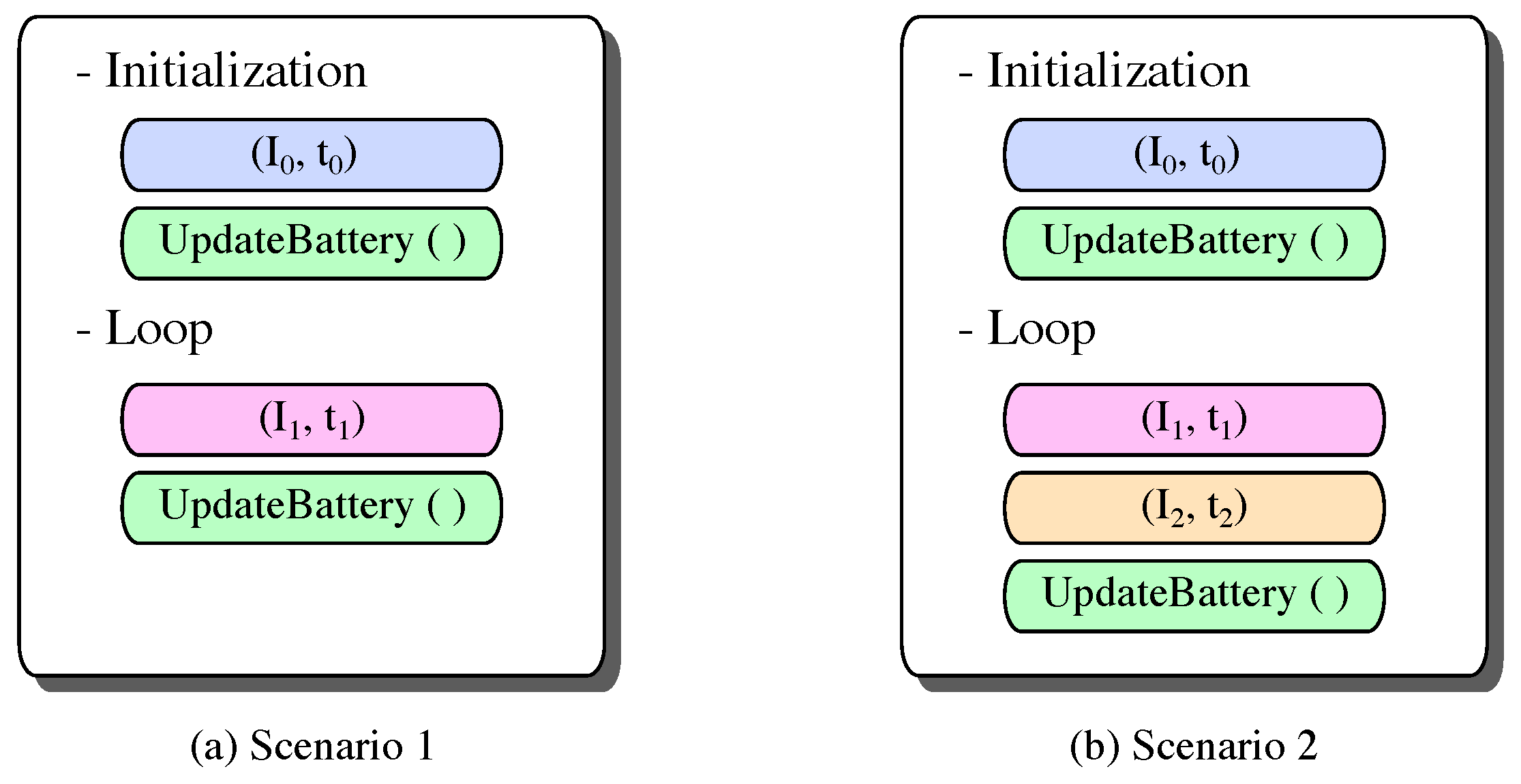Next, parameter $t_0$ represents the total battery lifetime. 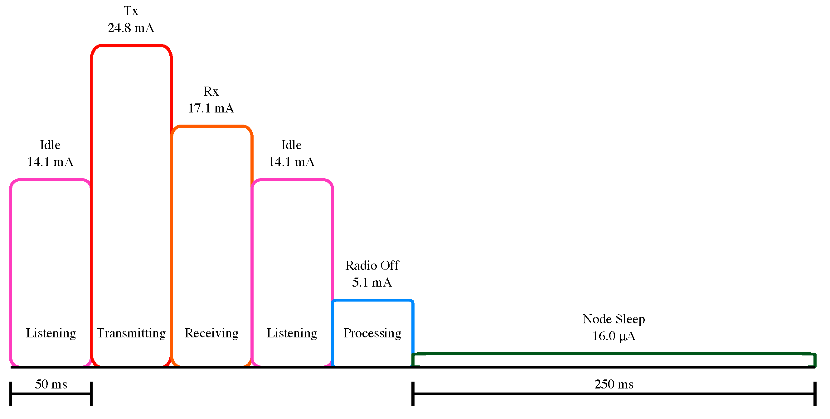In addition, parameter $D{P}_{set}$ may contain one or more pairs $(I_x,t_{I_x})$ to indicate the use of a set of tasks (i.e., a discharge profile as depicted in Figure 1). This feature is useful as a WSN node usually has different discharge currents for different operating states, e.g., Tx, Rx and Sleep. Using the $D{P}_{set}$ definition, duty cycles can also be used in the T-KiBaM implementation. In the TVM parameters, $prExp$ represents the initial value of the exponential voltage, $Exp\left(t_0\right)$, which is used for the calculation of $Exp\left(t\right)$ in each iteration.

In Algorithm 1, the correction factor (CF) function is applied in Line 1, as described in Section 3.2. In addition, the definition of k (Line 4) considers the Arrhenius equation values ($E_a$, A, R and T), which can be obtained through experiments (please refer to [16] for details). Through the for loop (Line 6), it becomes possible to call the T-KiBaM function according to the used discharge profile. As presented in Line 8, the user of T-KiBaM should check the content of the available charge tank, which needs to be greater than zero. This is a necessary condition for the battery operation, even if there is charge at the bound charge tank. Finally, note that the battery voltage level is obtained in Line 11, which performs the calculations corresponding to Equation (7). Finally, the algorithm returns some additional information about the battery, such as remaining battery charge in both tanks ($q_1$ and $q_2$), battery run time ($t_0$), and voltage level ($V_b$) when executing the discharge profile $D{P}_{set}$.

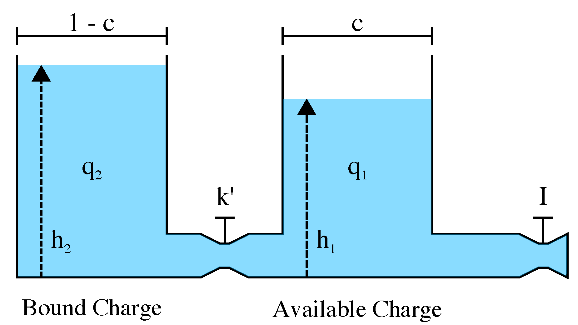
The T-KiBaM function implements the concepts presented in Section 3.1, where Equation (1) is used to calculate the charge of the battery over time. This stage returns the updated values in relation to the battery charge and its time of use. Algorithm 2 shows how to implement the T-KiBaM function.

Algorithm 2: T-KiBaM_function.

Input: c, k, $q_{1,0}$, $q_{2,0}$, $t_0$, I, $t_I$

Output: $q_1$, $q_2$, t

1 $q_0=q_{1,0}+q_{2,0}$;

2 $t=t_0+t_I$;

3 $q_1$ = compute-i ($c,k,q_0,q_{1,0},q_{2,0},I,t_I$);

4 $q_2$ = compute-j ($c,k,q_0,q_{1,0},q_{2,0},I,t_I$);

5 return ($q_1,q_2,t$);

The input parameters of the T-KiBaM function are as follows: c, k, $q_{1,0}$, $q_{2,0}$, $t_0$, I and $t_I$. The values of I and $t_I$ represent a task in the $D{P}_{set}$. Note that Lines 3 and 4 perform the calculations corresponding to Equation (1). The output values of $q_1$ and $q_2$ represent the actual state of charge in the available and bound charge tanks, respectively. Finally, t represents a time accumulator that is used to compute the total time of battery usage.

The knowledge about the SoC of the battery is very important for the development of energy-aware strategies. In this approach, during the node duty cycle, for example, it is possible to perform an iteration of T-KiBaM for each performed task (e.g., Tx, Rx, Sleep) in order to update the battery status (SoC and voltage level). With this, the node can take different decisions according to the current capacity of the battery. Although the proposed approach is flexible in several aspects, the following assumptions should be considered when running the T-KiBaM model:

• The node initializes its operating cycle with a fully charged battery, i.e., SoC = 100%. In addition, the T-KiBaM model is adjusted for the used battery technology. Therefore, it is not necessary to measure any battery information over time (e.g., voltage level);
• The node knows the discharge profile for all tasks that need to be performed during its operation. Knowing the discharge current in the transition between states, as well as the time it takes to perform such action, makes the T-KiBaM even more accurate. Thus, it is possible to parametrize T-KiBaM with the measured values and the time spent in each state/transition. In this case, the better the discharge profile definition, the greater the accuracy of the estimated battery behavior. Note that the discharge profile can be obtained from an analysis of the hardware power consumption (e.g., MCU, transceiver, sensors, etc.);
• The duty cycle of the node does not have to be constant since T-KiBaM supports different operating times ($t_{I_x}$) for each task ($I_x$), allowing the configuration of any combination of tasks;
• The node can obtain the environment temperature, which is provided to the T-KiBaM model to increase the accuracy of the estimate on the battery behavior.

An application example is presented in Section 6 to demonstrate the use of the T-KiBaM model.

4.2. Analytical vs. Experimental Comparison

The objective of this section is to validate the analytical evaluations comparing analytical results obtained from the T-KiBaM model with some experimental results, comparing the error between the two approaches regarding the battery lifetime estimation and its voltage behavior over time. Note that the values of all the constants of the T-KiBaM model were previously obtained by Rodrigues et al. [16]. In addition, all the analytical evaluations use the same experimental characteristics, such as discharge profile and temperature.

First, tests with continuous discharge currents were performed at different temperatures to evaluate the accuracy of the T-KiBaM model. The evaluated temperatures were as follows: $-5$, 10, 25, 32.5, and 40 ${}^{\circ }$C. The used discharge currents were 20 and 30 mA. With this, it became possible to analyze the relative Error (ERR) between analytical and experimental results.

Table 2. Battery lifetime *. EXP: Experimental result; T-KiBaM: analytical result; ERR: relative Error.

	$-5$ ${}^{\circ }$C			10 ${}^{\circ }$C			25 ${}^{\circ }$C			32.5 ${}^{\circ }$C			40 ${}^{\circ }$C
I (mA)	EXP (h)	T-KiBaM (h)	ERR (%)	EXP (h)	T-KiBaM (h)	ERR (%)	EXP (h)	T-KiBaM (h)	ERR (%)	EXP (h)	T-KiBaM (h)	ERR (%)	EXP (h)	T-KiBaM (h)	ERR (%)
20	36.714	36.866	0.41	37.402	37.361	0.11	37.984	37.814	0.45	37.835	37.976	0.37	37.133	37.271	0.37
30	24.749	24.750	0.00	25.087	25.082	0.02	25.385	25.386	0.00	25.560	25.495	0.26	25.022	25.022	0.00
AVG			0.20			0.06			0.22			0.31			0.18

* Results using continuous discharge currents.

presents the results of these evaluations. The experimental results (EXP), T-KiBaM and ERR columns represent, respectively, the experimental average lifetime of three battery measurements (note that the cutoff value of 2.0 V is considered for the calculation of the battery lifetime), the lifetime using T-KiBaM (in this case, the lifetime is reached when SoC $=0$%) and the relative error between EXP and T-KiBaM. The average ERR (AVG) values are presented at the of the table.

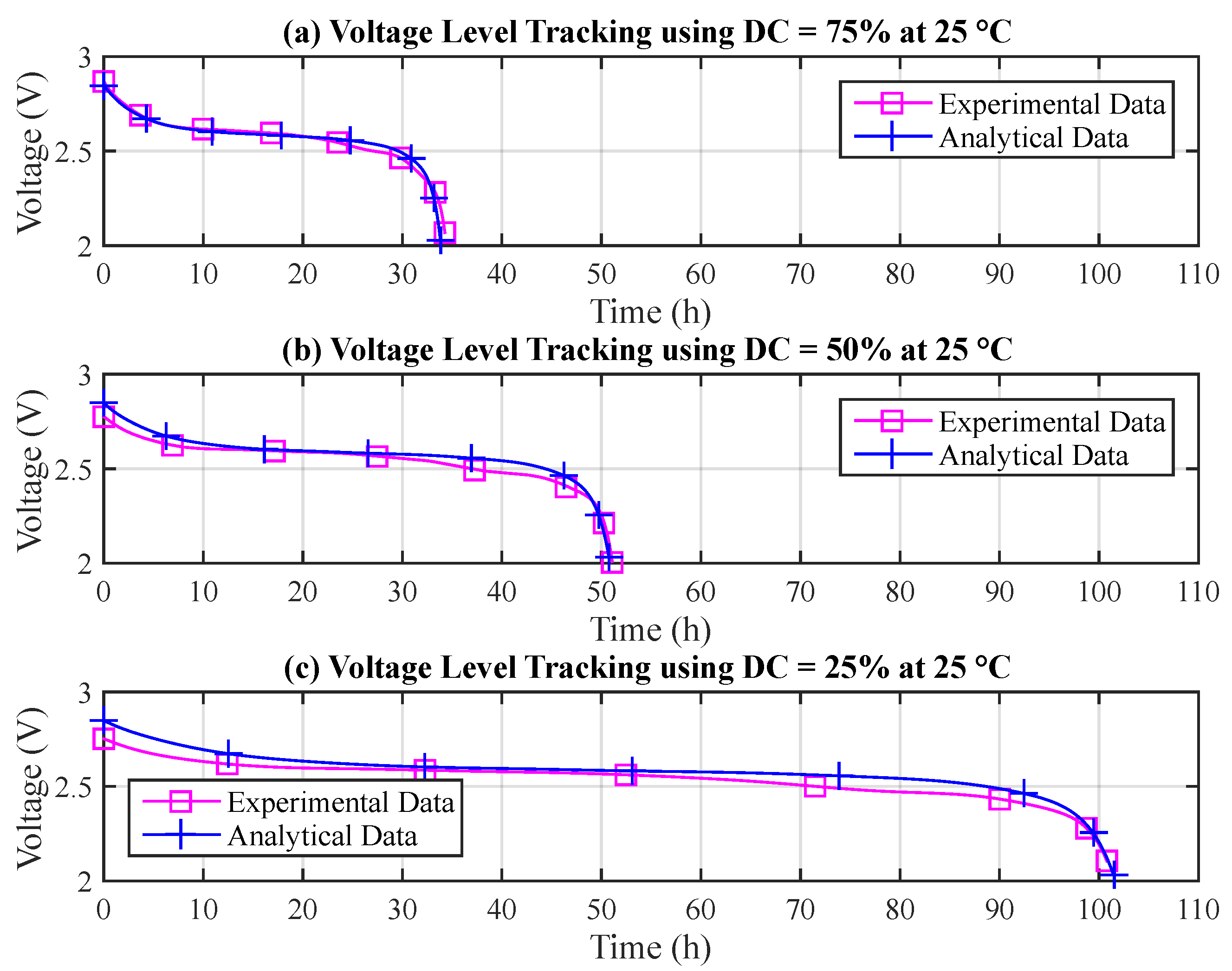
Next, some experiments using a Duty Cycle (DC) scheme were also carried out to evaluate the ability of the T-KiBaM model to handle typical WSN scenarios. The discharge current was set at 30 mA to decrease the time of the experiments. The following duty cycle schemes were evaluated:

$$\begin{array}{c}\hfill D{C}_{75\%}=[(I_1=30\mathrm{mA},t_{I_1}=3\mathrm{s});(I_2=0.0\mathrm{mA},t_{I_2}=1\mathrm{s})];\\ \hfill D{C}_{50\%}=[(I_1=30\mathrm{mA},t_{I_1}=1\mathrm{s});(I_2=0.0\mathrm{mA},t_{I_2}=1\mathrm{s})];\\ \hfill D{C}_{25\%}=[(I_1=30\mathrm{mA},t_{I_1}=1\mathrm{s});(I_2=0.0\mathrm{mA},t_{I_2}=3\mathrm{s})].\end{array}$$

Note that the duty cycle period is 4 s for $D{C}_{75\%}$ and $D{C}_{25\%}$, and 2 s for $D{C}_{50\%}$. In addition, only the temperature at 25 ${}^{\circ }$C was used in the experiments.

Table 3. Battery lifetime *. EXP: Experimental result; T-KiBaM: analytical result; ERR: relative Error.

	25 ${}^{\circ }$C
Duty Cycle (%)	EXP (h)	T-KiBaM (h)	ERR (%)
75	33.524	33.849	1.81
50	51.229	50.774	0.89
25	102.547	101.549	2.49
AVG			1.73

* Results using duty cycle schemes.

presents the results of this evaluation, including the relative Error for each situation.

These results demonstrate that T-KiBaM is able to accurately estimate the battery lifetime of WSN nodes, presenting average ERR values smaller than 0.35% for continuous discharge currents and an average ERR value of 1.73% for duty cycle schemes. However, although the presented results are quite accurate, battery lifetime is not the only interesting information that can be extracted from the T-KiBaM model.

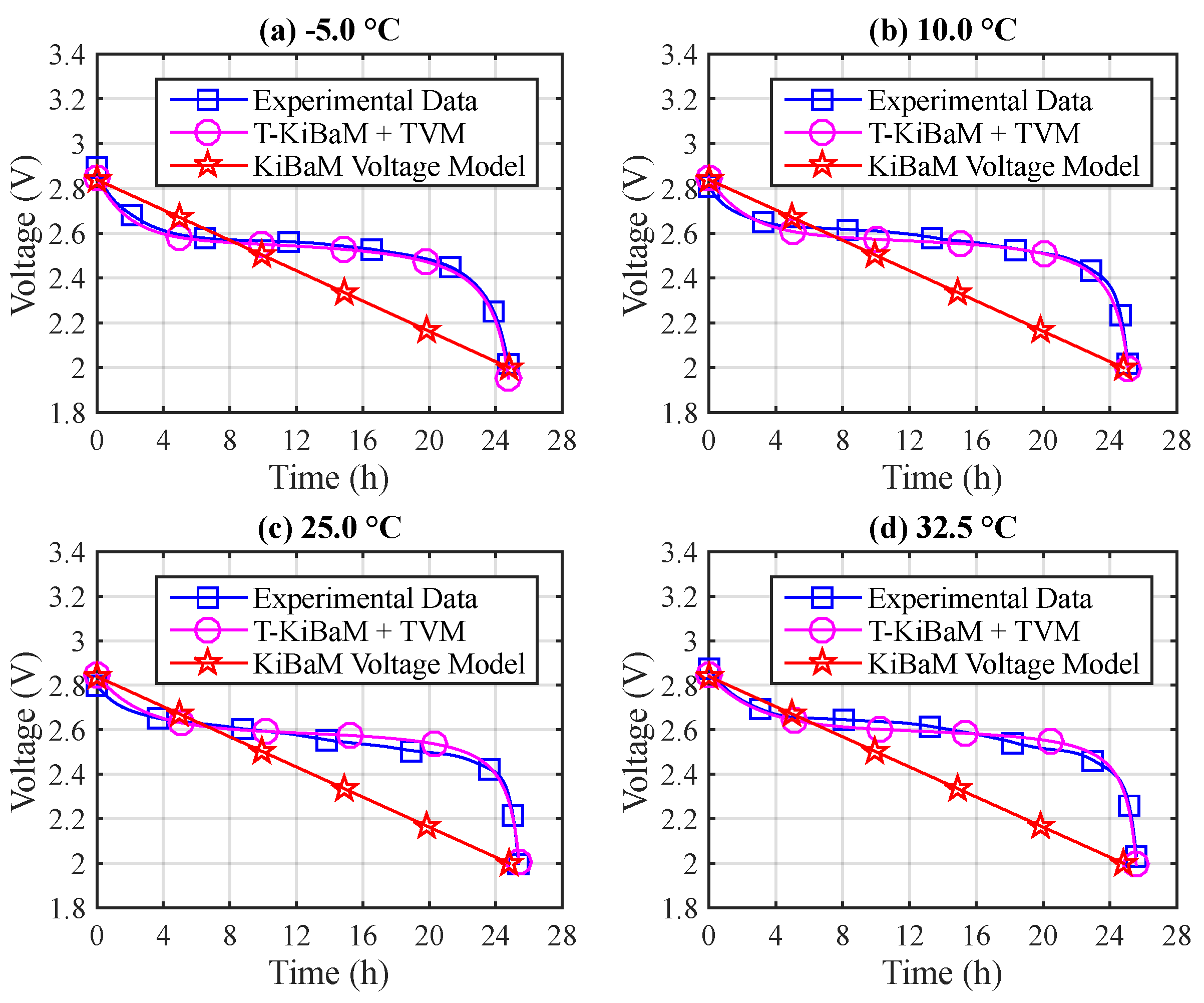
The voltage level is another relevant factor when evaluating the behavior of batteries. In the case of T-KiBaM, the battery voltage model provides voltage values that are dependent on the operating temperature, which allows monitoring the state of the battery more accurately, particularly, in WSN scenarios with high temperature variations. Figure 3 depicts an example comparing the experimental results using a continuous discharge current (30 mA) at different temperatures with those analytically obtained using the T-KiBaM and KiBaM models. The experimental data are fitted according to the average behavior of three experiments.

Note that the original KiBaM voltage model represents a linear battery discharge curve, $V\times t$. This type of approximation induces significant errors with respect to the lifetime analysis of any device connected to the battery. On the other hand, the T-KiBaM + TVM model offers a higher precision when estimating the behavior of the battery voltage curve over time. For instance, at T = −5 ${}^{\circ }$C (Figure 3a), analyzing the voltage level at 2.4 V, the relative error to the experiment of KiBaM is 37.53%, while in T-KiBaM is 0.73%.

5. Running T-KiBaM in Low-Power MCUs

This section presents the experimental results obtained when implementing the T-KiBaM model in multiple WSN-compatible MCUs. The objective is to check if analytical battery models, embedded in a low computational capacity hardware, can be used to track both the battery SoC and the voltage level of the battery itself over time. First, we present the basic characteristics of each MCU used in this work. Then, a discussion is included regarding the selected metrics used for the experimental evaluations. Finally, the results obtained from the experimental assessment are presented.

5.1. MCUs and Related Hardware Platforms

Arduino (https://www.arduino.cc) is an open-source platform that has been designed to facilitate electronic circuits prototyping. Arduino boards support the addition of sensors and/or actuators to existing designs, allowing the interaction with the physical environment. The use of this platform is highly popular due to its low cost, compatibility between operating systems, as well as the easy extensibility of both software and hardware. There are multiple Arduino board types. This work focuses on the UNO version that includes an Atmel ATmega328P low-power AVR 8-bit microcontroller, which has 32 KB of integrated Flash memory, as well as 2 KB of SRAM and 1 KB of EEPROM. This MCU operates at 16 MHz on the UNO board. The current consumption at 1 MHz is 0.2 mA in active mode [46]. Other MCUs were also used in the experimental assessments. These MCUs are using C code with specific manufacturer library (http://www.atmel.com/tools/avrsoftwareframework.aspx). The specifications of each used micro-controller are summarized in

Table 4. Specifications of the used MCUs.

MCU	Platform	Clock (MHz)	Wait State	FPU	Flash (KB)	SRAM (KB)	EEPROM (KB)	Typical Current (mA)
ATmega328P	8-bit AVR	16	0	no	32	2	1	0.2
ATmega128RFA1	8-bit AVR	16	0	no	128	16	4	4.1
ATxmega256A3U	8/16-bit AVR	32	0	no	256	16	4	9.5
SAMR21G18A	32-bit ARM Cortex-M0+	48	1	no	256	32	0	6.7
SAMG55	32-bit ARM Cortex-M4	120	5	yes	512	160	0	24.2
SAMV71Q21	32-bit ARM Cortex-M7	300	6	yes	2048	384	0	83.0

.

The Atmel ATmega128RFA1 is an 8-bit AVR MCU, which has a built-in 128 KB of Flash memory, as well as 16 KB of SRAM and 4 KB of EEPROM. The MCU can operate up to 16 MHz [47]. The Atmel ATxmega256A3U is an 8/16-bit AVR XMEGA low-power MCU that features 256 KB of Flash memory, as well as 16 KB of SRAM and 4096 bytes of EEPROM. This MCU can run at 32 MHz [48]. The Atmel SAMR21G18A MCU uses a low-power 32-bit ARM Cortex-M0+ processor. This chip has a 256 KB of Flash memory, plus 32 KB of SRAM [49]. The Atmel SAMG55 is based on the ARM architecture. This MCU has a 32-bit Cortex-M4 core that can reach speeds up to 120 MHz with a Floating Point Unit (FPU). In addition, this chip has 512 KB Flash Memory and 160 KB SRAM plus up to 16 KB (cache + I/D RAM) [50]. The Atmel SMART SAMV71Q21 is based on the ARM architecture, featuring a Cortex-M7 RISC 32-bit processor with a FPU. This MCU can reach speeds up to 300 MHz, featuring 2048 KB of Flash memory, as well as a dual 16-KB cache and 384 KB of SRAM memories [51].

5.2. Performance Metrics

As the results presented in Section 4 are consistent with those found in the experimental assessment, i.e., T-KiBaM parameters have been properly adjusted, a computer with a 2.9 GHz Intel Core i5 processor running MATLAB is used as the basis of the comparisons regarding the battery lifetime estimation. This is considered the best platform for the execution of this algorithm as it presents an interesting precision regarding the number of significant figures. Thus, the tested set includes the same experimental continuous discharge currents, as well as a variety of other discharge current values. Such set comprises the following currents: 5, 10, 20, 30, 40, 50, 60, 70, 80, 90, and 100 mA.

The following metrics are used for this experimental assessment: (i) algorithm execution time; (ii) memory usage; (iii) energy consumption; (iv) number of iterations of the algorithm for different tasks; and (v) estimated battery lifetime.

5.3. Experimental Results Using Low-Power MCUs

The results shown in this section were obtained by running the T-KiBaM functions on different low-power MCUs. Note that, when using continuous discharge currents in the analytical evaluations, the T-KiBaM function needs an operating time $t_I$ (or time step) as input to run the battery model. Hereafter, a 1-second step was assumed between consecutive executions as it represents a relevant low granularity when continuous discharge currents are used to feed the model, if compared to the total battery discharge time. A discussion regarding the time step size is performed in Section 6.3.

5.3.1. Execution Time

The first evaluated metric is the function execution time (ET) when running T-KiBaM in low-power MCUs. The objective is to compare the performance of the algorithm in platforms with different characteristics in order to verify the possibility of its implementation in WSN nodes.

It is important to note that the results presented in this section consider the average of three executions of the algorithm. The execution times were collected from checkpoints at the beginning and at the end of the T-KiBaM function call. In addition, all micro-controllers can only access the flash memory with a maximum clock of 32 MHz and, after that speed, wait-states must be inserted. All the performed experiments used the best configuration to achieve the fastest results. Note that the focus of this work is not on the evaluation of the faster micro-controller, therefore, the source code was compiled with -O2 option and no specific optimization was performed in the available libraries. The FPU has been enabled in all MCUs with this option. The instruction cache has been enabled in SAMG55 and the instruction/data cache have been enabled in SAMV71. The use of same MCU manufacturer allowed both to unify code and test the same library for all MCU models.

Table 5. Execution times (average) on all platforms *.

	ATmega 328P	ATmega 128RFA1	ATxmega 256A3U	SAMR 21G18A	ATSAM G55	SAMV 71Q21
Execution Time ($\mathsf{\mu }$s)	549.02	499.86	259.10	1311.65	164.87	5.33

* Results using the clock frequencies shown in Table 4.

presents the average execution times achieved by each platform.

The results point to average execution times of less than 1.4 ms on all platforms. The SAMV71Q21 micro-controller presented an average execution time close to 5.3 $\mathsf{\mu }$s. This result is within the expected range, since this MCU operates at a higher frequency, i.e., 300 MHz. On the other hand, the SAMR21G18A micro-controller delivers a poor performance for a MCU from its category. The average execution time around 1.3 ms, even when operating at 48 MHz, could be related to lack of code optimization of GCC compiler [52] that increases code size and, consequently, slows down the code execution considerably. The performed experiments clarified that optimization should be mandatory to achieve better results. Tests also have shown that ARM and AVR produce similar results when using soft float ABI (Application Binary Interface) and no cache since ARMs, probably, are stalled waiting for new instruction due to wait-states. Despite this, the rational indicates that the obtained values are feasible when compared with real-world applications, such as the use of encryption algorithms in WSNs with low-power MCUs [26].

5.3.2. Memory Usage

The second evaluated metric is memory usage. Analyzing the amount of Flash memory occupied by the T-KiBaM model is an important metric, as micro-controllers used in WSN nodes usually have very little available memory. In this sense, it is possible to establish the spatial cost of implementing an analytical battery model in a low-power MCU.

Note that the results presented in this section consider only the memory usage relative to the T-KiBaM model source code implementation and the essential compile components on each platform. In other words, libraries and debugging codes are not considered in this analysis.

Table 6. Memory usage on all platforms.

	ATmega 328P	ATmega 128RFA1	ATxmega 256A3U	SAMR 21G18A	ATSAM G55	SAMV 71Q21
Memory usage (KB)	7.444	11.384	19.254	40.376	39.136	25.712
Total Available (KB)	32	128	256	256	512	2048
Percentage of total (%)	23.0	8.9	7.5	15.7	7.6	1.2

presents the memory usage on all platforms, including the percentage of total available memory.

According to Table 6, the implementation of T-KiBaM on the SAMR21G18A occupies approximately 40.3 KB, the highest memory occupancy among all platforms. On the other hand, the ATmega328P presents the lowest memory occupancy, with only 7.4 KB. However, in relation to the total Flash memory availability, this micro-controller has the highest occupancy, about 23.0% of 32 KB in total. The SAMV71Q21 has the lowest memory occupancy rate in percentage terms.

As observed in Table 6, three of the five tested platforms have memory occupancy rates of less than 10%. Thus, these results show that it is feasible to implement an analytical battery model on a low-power WSN node, such as the iLive node [53] which features 128 KB of Flash memory.

5.3.3. Power Consumption

The power consumption is the third metric evaluated in this work. The objective is to evaluate how much energy consumes an iteration of the T-KiBaM algorithm. For this, it is necessary to measure the current consumed by each MCU first. Further details are given below.

A multimeter (MD-6450 True-RMS) was used to measure the current on each platform. All measurements were taken with the board of each micro-controller connected via USB while running the T-KiBaM model. Voltage variations are not considered since the algorithm execution time is very small (<1.4 ms). Thus, the average values for voltage (≈5.05 V) and current are considered in the calculations of this section.

Table 7. Power consumption in each platform.

	ATmega 328P	ATmega 128RFA1	ATxmega 256A3U	SAMR 21G18A	ATSAM G55	SAMV 71Q21
Power Supply (V)	5.05	5.05	5.05	5.05	5.05	5.05
Current(mA)	49.3	77.1	18.9	12.0	30.2	82.6
Power (mW)	248.9	389.3	95.4	60.6	52.5	417.1

shows the measured current values as well as the electrical power for each micro-controller, calculated through the relation $P=V\times I$.

From these results, it is possible to obtain the energy spent according to the execution time of an iteration of T-KiBaM algorithm in each micro-controller, through the relation $E=P\times \Delta t$. In this case, $\Delta t$ is obtained from the execution time in each platform. Therefore, the energy spent is directly related to the first metric, the execution time.

Table 8. Energy spent (average) on a single iteration of the algorithm on all platforms.

	ATmega 328P	ATmega 128RFA1	ATxmega 256A3U	SAMR 21G18A	ATSAM G55	SAMV 71Q21
Energy Spent (mJ)	0.1366	0.1945	0.0247	0.0794	0.0086	0.0022

shows the average energy spent when running a single iteration of T-KiBaM on each platform.

6. T-KiBaM Usage in WSN Nodes: Application Example

WSN nodes usually perform several tasks during their operation, including data transmission (Tx), reception (Rx) and processing (Pr). It is also possible to save energy during certain intervals of time by putting the nodes in sleep mode (Sl). Generally speaking, such nodes operate in duty cycle scheme, i.e., cyclically repeating a sequence of tasks over time, until their battery power runs out. The objective of this section is to illustrate the usage of T-KiBaM in a real application, considering the operating characteristics of real WSN nodes. With this, other performance metrics can be assessed in relation to the execution of the T-KiBaM model in low-power MCUs. Finally, the presented application example is used in a sensitivity analysis, where variations are applied to the input parameters of the T-KiBaM model.

6.1. Application Example

The application scenario described in this section cover the mode of operation of most WSN applications. In this sense, two scenarios are described: (i) the node remains 100% of the time in the active mode; and (ii) the node operates in a duty cycle scheme, i.e., inserting periods in sleeping mode alternately with its active period. Further details are given below.

A set of tasks (discharge profile) can be used to properly emulate the operation of the nodes, i.e., discharge the battery charge when performing different tasks. However, to simplify the analysis, it is assumed that the node performs only one useful task (e.g., Rx, Tx, or Pr) in both scenarios. A task is defined by the discharge current and its operating time (I, $t_I$), including periods in sleeping mode. The node executes the T-KiBaM algorithm at the end of its task to update the state of charge of its battery. Although it may play a significant role in energy consumption, the node initialization process is not considered in these analysis, since it runs only once during its entire life cycle. Figure 4 depicts a schematic summarizing the node activities in the two presented scenarios.

As depicted in Figure 4a, Scenario 1 presents the operating mode of a node operating 100% of the time in active mode. Note that the main loop considers only the performed task, represented by $(I_1,t_1)$, and the update of the battery state of charge and voltage level. On the other hand, Figure 4b presents Scenario 2, which adds a sleep mode period, represented by $(I_2,t_2)$, at each duty cycle. In this sense, the node performs its main task, goes into low-power mode (Sl), and then updates the battery state of charge and voltage level.

6.2. Estimating the Battery Lifetime

The fourth metric assessed in this work is the battery lifetime estimation. One of the main features of T-KiBaM model is to provide the estimated battery lifetime according to the used discharge profile. Therefore, a modified version of Algorithm 1 was considered to allow the cyclic execution of the discharge profile, i.e., as a duty cycle scheme, until the battery charge runs out. Through this simple modification, it becomes possible to predict the total battery lifetime according to both the discharge profile and the operating temperature. Scenarios 1 and 2 are used in these assessments as they depict the operating mode of traditional WSN nodes. The evaluations performed in this section consider the aspects below.

The first requirement to evaluate the battery lifetime estimation is to run the T-KiBaM model until the battery charge runs out. In these evaluations, the selected cutoff point occurs when the T-KiBaM algorithm indicates SoC $=0\%$ (≈2.0 V). It is worth mentioning that other cutoff points can be selected depending on the hardware requirements (e.g., 2.1 V or 2.2 V).

The second aspect concerns the tested set of tasks, which is the same as mentioned in Section 5.2 for Scenario 1. For simplification purposes, the experiments using Scenario 2 assume that the sleep mode does not consume energy (i.e., $I_2=0.0$ mA), although it is recognized that there is a small discharge current in this state, usually in the range of $\mathsf{\mu }$A [54].

The last aspect concerns the number of iterations required for the algorithm to complete the estimation over the battery lifetime. In this case, the lower the granularity of the operating times ($t_{I_x}$) of the discharge currents ($I_x$), the greater the number of iterations of the algorithm and, consequently, the longer its computation time. Figure 5a depicts the number of iterations after performing the T-KiBaM model until the battery charge runs out for each discharge current presented in the mentioned set of tasks.

Considering the previously mentioned aspects, the challenge of this evaluation is to assess how close the estimates of the battery lifetime are from the results obtained when executing the T-KiBaM model in a PC. The assessments for both Scenarios 1 and 2 are presented below.

For the Scenario 1 assessments, the entire set of tasks (i.e., $I_1=5,10,20,30,40,\dots ,100$ mA) is executed with $t_1=1$ s.

Table 9. Estimated battery lifetime *. ELT: Estimated Lifetime; EXP: Experimental time.

${\mathit{I}}_1$ (mA)	ATmega 328P ELT (h)	ATmega128 RFA1 ELT (h)	ATxmega256 A3U ELT (h)	SAMR21 G18A ELT (h)	ATSAM G55 ELT (h)	SAMV71 Q21 ELT (h)	MATLAB ELT (h)	EXP (h)
5	153.1517	153.1517	153.1517	153.4969	153.4969	153.4969	153.5533	-
10	73.7003	73.7003	73.7003	73.6264	73.6264	73.6264	73.6536	73.557
20	37.8050	37.8050	37.8050	37.8028	37.8028	37.8028	37.8150	37.984
30	25.3956	25.3956	25.3956	25.3764	25.3764	25.3764	25.3869	25.385
40	19.1914	19.1914	19.1914	19.1850	19.1850	19.1850	19.1936	-
50	15.3572	15.3572	15.3572	15.3575	15.3575	15.3575	15.3550	-
60	12.7958	12.7958	12.7958	12.7947	12.7947	12.7947	12.7956	-
70	10.9658	10.9658	10.9658	10.9667	10.9667	10.9667	10.9675	-
80	9.5961	9.5961	9.5961	9.5953	9.5953	9.5953	9.5967	-
90	8.5328	8.5328	8.5328	8.5300	8.5300	8.5300	8.5303	-
100	7.6775	7.6775	7.6775	7.6778	7.6778	7.6778	7.6772	-

* Results considering Scenario 1 in all platforms.

presents the results regarding the estimated battery lifetime obtained when running the T-KiBaM algorithm on all platforms using Scenario 1. Note that the EXP column represents the results obtained when using real batteries at 25 ${}^{\circ }$C, when available.

The results indicate small relative Errors when compared to the estimated battery lifetime on a PC running MATLAB. For instance, considering all tested discharge currents, the average deviation between the ATmega328P and MATLAB is 0.042%. In this case, the minimum relative Error is 0.002% and the maximum relative Error is 0.262% (when $I_1=5$ mA). Figure 5b depicts the relative error of the ATmega328P with respect to the estimated battery lifetime when using T-KiBaM on MATLAB for the entire set of discharge currents. The other MCUs present the following average relative Errors: 0.042% (ATmega128RFA1), 0.042% (ATxmega256A3U), 0.023% (SAMR21G18A), 0.023% (ATSAMG55) and 0.023% (SAMV71Q21).

The evaluations for Scenario 2 consider the insertion of sleeping periods between the activities of the node, which operates in a duty cycle (DC) scheme. In this case, the evaluated duty cycles are as follows: 100%, 75%, 50%, 25%, 10%, and 5%. The discharge current ($I_1$) has its value set at 30 mA to allow comparison with the experimental results. Thus, the used current profiles are as follows:

$$\begin{array}{cc}D{C}_{100\%}=[(30\mathrm{mA},1\mathrm{s});(0.0\mathrm{mA},0\mathrm{s})],\hfill & \hfill D{C}_{75\%}=[(30.0\mathrm{mA},3\mathrm{s});(0.0\mathrm{mA},1\mathrm{s})],\\ D{C}_{50\%}=[(30.0\mathrm{mA},1\mathrm{s});(0.0\mathrm{mA},1\mathrm{s})],\hfill & \hfill D{C}_{25\%}=[(30.0\mathrm{mA},1\mathrm{s});(0.0\mathrm{mA},3\mathrm{s})],\\ D{C}_{10\%}=[(30.0\mathrm{mA},1\mathrm{s});(0.0\mathrm{mA},9\mathrm{s})],\hfill & \hfill D{C}_{5\%}=[(30.0\mathrm{mA},1\mathrm{s});(0.0\mathrm{mA},19\mathrm{s})].\end{array}$$

Since the results between the platforms for Scenario 1 are very close, the evaluations for Scenario 2 are performed only with the ATmega328P MCU.

Table 10. Estimated battery lifetime *. ELT: Estimated Lifetime; EXP: Experimental time.

Duty Cycle (%)	ATmega 328P ELT (h)	MATLAB ELT (h)	EXP (h)
100	25.3956	25.3869	25.385
75	33.8533	33.8489	33.524
50	50.7678	50.7744	51.229
25	101.6122	101.5489	102.547
10	253.8528	253.8722	-
5	507.3667	507.7444	-

* Results considering Scenario 2 in ATmega328P.

presents the results obtained after running the T-KiBaM algorithm on this platform using Scenario 2. Again, the EXP column represents the results obtained from experiments with real batteries at 25 ${}^{\circ }$C, when available.

The results illustrated in Table 10 demonstrate that the estimates for the battery lifetime are compatible on both platforms. The variations in the results arise by virtue of the accuracy of the numerical representation in each platform. Regarding the voltage level tracking, Figure 6 depicts the behavior of the battery discharge curves for duty cycles of 75%, 50% and 25% at 25 ${}^{\circ }$C. The experimental data represents the average behavior obtained in the experimental assessments, being presented as fitted curves. The analytical results are obtained through data prints during the execution of the T-KiBaM algorithm, however, only the fitted curves are presented for easy viewing.

6.3. Sensibility Analysis of T-KiBaM Model with Different Time Step Values

Finally, this section presents an assessment of the same application example, when different values are considered for the time step ($t_{I_x}$) of the discharge current ($I_x$) in the T-KiBaM function. The objective is to assess the relationship between the execution time of the algorithm for different tasks and the quality of the estimation prediction with respect to the battery operating behavior, i.e., its lifetime and voltage level over time, in Scenario 1. Note that the time step value corresponds to the interval between two consecutive invocations of the battery update function. The following time steps are used for this assessment: 1, 2, 5, 10 and 60 s. This assessment is performed only for the ATmega328P, as this micro-controller presents the hardware with the least amount of available resources among all the previously assessed devices. Thus, these results can be similarly extended to the other platforms.

First, the quality of the estimated battery lifetime is evaluated for different time steps. In this sense, the following metrics are evaluated: (i) execution time; (ii) number of iterations and (iii) estimated battery lifetime. The assessments considering Scenario 1 are performed below.

The first evaluated metric is the execution time for the entire set of tasks when different time steps are used as input to the T-KiBaM function. Figure 7a depicts the results obtained for the set of discharge currents mentioned in Section 5.2. Note that the execution time of each task $(I_x,t_{I_x})$ reduces dramatically, as the discharge current time step increases. For example, by comparing the time steps of 1 s and 10 s when $I_1=5$ mA, the execution time falls from 303.98 s to 32.227 s when the algorithm is executed until the battery charge runs out. Considering the entire set of tasks, it is possible to observe an execution time 9.5 times faster, on average. The same behavior is observed for the second metric, i.e., the number of iterations, as shown in Figure 7b. Using the same time steps mentioned in the previous example, 1 s and 10 s, the number of iterations drops from 551,347 to 55,320, respectively. Considering the entire set of tasks, it is possible to observe a reduction in the number of iterations equivalent to 10 times, on average.

The third evaluated metric is the estimated battery lifetime when different time steps are used as input to the T-KiBaM function. Figure 8a depicts the results obtained for the same set of discharge currents. As expected, the estimated battery lifetime has small variations for all the assessed cases.

Clearly, in terms of resource savings and performance, WSN designers should select the highest time step values. However, this selection must also take into account the imprecision introduced in the estimation when large time intervals are used to make the measurements. Figure 8b depicts the relative error for each time step considering the results obtained in a PC regarding the selected set of discharge currents. Note that the relative error is less than 0.4% for all the assessed cases. Particularly, the time step equal to 2 s has the highest relative errors for tasks with low discharge currents (<50 mA). On the other hand, the time step equal to 60 s presents highest relative error for tasks with larger discharge currents (>50 mA). According to these evaluations, the time step equal to 10 s is most indicated when continuous discharge currents are evaluated by the T-KiBaM model, since both the execution time and the number of iterations are significantly smaller and, at the same time, both the average relative error and the standard deviation compared to the values estimated in the PC are the lowest.

Finally, the voltage level estimation provided by the T-KiBaM model is evaluated over time, using different time steps (Scenario 1). Again, a comparison of the experimental and analytical results is performed, using the results provided by the ATmega328P MCU at the time steps mentioned above. Figure 9 depicts the behavior of the estimation of the voltage curve at each update of the T-KiBaM model, under a continuous discharge current of 30 mA, at $-5$ ${}^{\circ }$C. The experimental data are adjusted according to the average behavior of three experiments.

Note that the assessments done for the ATmega328P present the same results of the analytical evaluation performed on the PC, regardless the used time step. Thus, it is clear that the T-KiBaM model generates compatible results for both low-power and robust platforms regarding the voltage level tracking. This is a major result as estimating the voltage level over time is required to ensure the operation of any sensor node, allowing for optimizations in the WSN management policies.

7. Conclusions

Estimating the battery lifetime is a complex task since many factors can influence the battery behavior, e.g., technology, operating temperature and discharge current. Analytical battery models may assist in this task, achieving results close to reality. However, two problems may arise within the WSN context. Firstly, the implementation of complex analytical models upon low-capacity hardware platforms is not an easy task, due to low processing capability, memory constraints and the high accuracy required to represent low varying analog values. Secondly, the execution of this type of analytical models by real-world nodes will influence its energy consumption, and therefore, the required effort to estimate the network lifetime may reduce the lifetime of the network itself.

The study performed in this paper evaluated the cost of executing an analytical battery model known as T-KiBaM in low-power MCUs. The model validation took into account experimental data. As shown in Section 4, the T-KiBaM model can accurately estimate the lifetime of Ni-MH batteries and is also able to estimate the voltage behavior over time at different temperatures, which is an important issue when considering devices (nodes) that require a minimum voltage value to maintain their operation. The analytical models were implemented upon different micro-controllers. As a result, although running T-KiBaM on low-power MCUs requires long computing times, such computing times do not represent a significant slice of the estimated battery lifetime. Therefore, the time required to estimate the battery behavior (which includes tracking both its SoC and voltage level over time) is feasible.

As future work, we are interested in finding a way to integrate the knowledge about both the discharge current and voltage level of the battery [36,55] to feed the T-KiBaM in real time, similar to the use of a fuel gauge IC in a smart battery pack. In this sense, it would become possible to implement a closed-loop approach, allowing the correction of predictions over time. Other issues will also be addressed in future work, such as a full research on the use of duty cycle discharge profiles at different temperatures. The validation of the estimates can also be made through the implementation of the proposed battery model in sensor nodes of a physical WSN. In this case, an application with a basic set of tasks should be used to allow the construction of a well-known fixed discharge profile. This would ensure minimal variability over the node’s activities so that the results could be fairly comparable. Finally, the influence of the aging effect on sensor node batteries should be included in the proposed battery model to improve both the management and maintenance issues in WSNs.

References

1. Kim, T.; Qiao, W. A hybrid battery model capable of capturing dynamic circuit characteristics and nonlinear capacity effects. IEEE Trans. Energy Convers. 2011, 26, 1172–1180. [Google Scholar] [CrossRef]
2. Wang, Y.; Zhang, C.; Chen, Z. A Method for state-of-charge estimation of LiFePO4 batteries at dynamic currents and temperatures using particle filter. J. Power Sources 2015, 279, 306–311. [Google Scholar] [CrossRef]
3. Lajara, R.J.; Perez-solano, J.J.; Pelegrí-sebastia, J. A method for modeling the battery state of charge in wireless sensor networks. IEEE Sens. J. 2015, 15, 1186–1197. [Google Scholar] [CrossRef]
4. Gandolfo, D.; Brandão, A.; Patiño, D.; Molina, M. Dynamic model of lithium polymer battery–Load resistor method for electric parameters identification. J. Energy Inst. 2015, 88, 470–479. [Google Scholar] [CrossRef]
5. Buchli, B.; Aschwanden, D.; Beutel, J. Battery state-of-charge approximation for energy harvesting embedded systems. In Wireless Sensor Networks (EWSN); Demeester, P., Moerman, I., Terzis, A., Eds.; Springer: Berlin/Heidelberg, Germany, 2013. [Google Scholar]
6. Che, Z.; Jin, R.; Zhu, M.; Wang, Z.; Wang, L. Battery optimal scheduling based on energy balance in wireless sensor networks. IET Wirel. Sens. Syst. 2015, 5, 277–282. [Google Scholar]
7. Wang, Y.; Yang, D.; Zhang, X.; Chen, Z. Probability based remaining capacity estimation using data-driven and neural network model. J. Power Sources 2016, 315, 199–208. [Google Scholar] [CrossRef]
8. Rahimi-Eichi, H.; Ojha, U.; Baronti, F.; Chow, M.Y. Battery management system: An overview of its application in the smart grid and electric vehicles. IEEE Ind. Electron. Mag. 2013, 7, 4–16. [Google Scholar] [CrossRef]
9. Smart Battery System Implementers Forum. Smart Battery Data Specification–Addendum for Fuel Cell Systems. 2007. Available online: http://sbs-forum.org/specs/sbdata_addendum_fuel_cells_20070411.pdf (accessed on 31 March 2017).
10. Cadex Electronics Inc. Smart Battery Technolog. 2017. Available online: http://www.cadex.com/en/batteries/smart-battery-technology (accessed on 31 March 2017).
11. Maxim Integrated. DS2780 Standalone Fuel Gauge IC. Available online: https://datasheets.maximintegrated.com/en/ds/DS2780.pdf (accessed on 18 April 2017).
12. Razaque, A.; Elleithy, K. Energy-efficient boarder node medium access control protocol for wireless sensor networks. Sensors 2014, 14, 5074–5117. [Google Scholar] [CrossRef] [PubMed]
13. Jabbar, S.; Minhas, A.A.; Imran, M.; Khalid, S.; Saleem, K. Energy efficient strategy for throughput improvement in wireless sensor networks. Sensors 2015, 15, 2473–2495. [Google Scholar] [CrossRef] [PubMed]
14. Mammu, A.S.I.K.; Hernandez-Jayo, U.; Sainz, N.; de la Iglesia, I. Cross-layer cluster-based energy-efficient protocol for wireless sensor networks. Sensors 2015, 15, 8314–8336. [Google Scholar] [CrossRef] [PubMed]
15. Jongerden, M.R.; Haverkort, B.R. Battery Modeling; Technical Report; University of Twente: Enschede, Netherlands, 2008. [Google Scholar]
16. Rodrigues, L.M.; Montez, C.; Moraes, R.; Portugal, P.; Vasques, F. A temperature-dependent battery model for wireless sensor networks. Sensors 2017, 17, 422. [Google Scholar] [CrossRef] [PubMed]
17. Atmel Corporation. Home Page. Available online: http://www.atmel.com (accessed on 2 June 2017).
18. Cheng, P.; Zhou, Y.; Song, Z.; Ou, Y. Modeling and SOC estimation of LiFePO4 battery. In Proceedings of the IEEE International Conference on Robotics and Biomimetics (ROBIO), Qingdao, China, 3–7 December 2016. [Google Scholar]
19. Wang, Y.; Zhang, C.; Chen, Z. A method for state-of-charge estimation of Li-Ion batteries based on multi-model switching strategy. Appl. Energy 2015, 137, 427–434. [Google Scholar] [CrossRef]
20. Zhu, Q.; Xiong, N.; Yang, M.L.; Huang, R.S.; Hu, G.D. State of charge estimation for Lithium-Ion battery on nonlinear observer: An Hinf method. Energies 2017, 10, 1–19. [Google Scholar] [CrossRef]
21. Hannan, M.A.; Lipu, M.S.H.; Hussain, A.; Mohamed, A. A review of Lithium-Ion battery state of charge estimation and management system in electric vehicle applications: Challenges and recommendations. Renew. Sustain. Energy Rev. 2017, 78, 834–854. [Google Scholar] [CrossRef]
22. Çakiroğlu, M. Software implementation and performance comparison of popular block ciphers on 8-bit low-cost microcontroller. Int. J. Phys. Sci. 2010, 5, 1338–1343. [Google Scholar]
23. Liu, W.; Luo, R.; Yang, H. Cryptography overhead evaluation and analysis for wireless sensor networks. In Proceedings of the WRI International Conference on Communications and Mobile Computing, Yunnan, China, 6–8 January 2009; pp. 496–501. [Google Scholar]
24. Capo-Chichi, E.P.; Guyennet, H.; Friedt, J.M. K-RLE: A new data compression algorithm for wireless sensor networks. In Proceedings of the International Conference on Sensor Technologies and Applications (SENSORCOMM), Athens, Greece, 18–23 June 2009; pp. 502–507. [Google Scholar]
25. Guo, H.; Low, K.S.; Nguyen, H.A. Optimizing the localization of a wireless sensor network in real time based on a low-cost microcontroller. IEEE Trans. Ind. Electron. 2011, 58, 741–749. [Google Scholar] [CrossRef]
26. Othman, S.B. Performance evaluation of encryption algorithm for wireless sensor networks. In Proceedings of the International Conference on Information Technology and e-Services (ICITeS), Sousse, Tunisia, 24–26 March 2012; pp. 1–8. [Google Scholar]
27. Quirino, G.S.; Moreno, E.D.; Matos, L.B.C. Performance evaluation of asymmetric encryption algorithms in embedded platforms used in WSN. In Proceedings of the World Congress in Computer Science, Computer Engineering and Applied Computing (WORLDCOMP), Las Vegas, NV, USA, 22–25 July 2013. [Google Scholar]
28. Pardo, J.; Zamora-Martínez, F.; Botella-Rocamora, P. Online learning algorithm for time series forecasting suitable for low cost wireless sensor networks nodes. Sensors 2015, 15, 9277–9304. [Google Scholar] [CrossRef] [PubMed]
29. Panić, G.; Stecklina, O.; Stamenković, Z. An embedded sensor node microcontroller with crypto-processors. Sensors 2016, 16, 607. [Google Scholar] [CrossRef] [PubMed]
30. Leveque, A.; Pecheux, F.; Louerat, M.M.; Aboushady, H.; Vasilevski, M. SystemC-AMS models for low-power heterogeneous designs: Application to a WSN for the detection of seismic perturbations. In Proceedings of the International Conference on Architecture of Computing Systems (ARCS), Hannover, Germany, 22–25 February; pp. 1–6.
31. Biswas, K.; Muthukkumarasamy, V.; Wu, X.W.; Singh, K. An analytical model for lifetime estimation of wireless sensor networks. IEEE Commun. Lett. 2015, 19, 1584–1587. [Google Scholar] [CrossRef]
32. Kim, J.U.; Kang, M.J.; Yi, J.M.; Noh, D.K. A simple but accurate estimation of residual energy for reliable WSN applications. Int. J. Distrib. Sens. Netw. 2015, 2015. [Google Scholar] [CrossRef]
33. Dron, W.; Duquennoy, S.; Voigt, T.; Hachicha, K.; Garda, P. An emulation-based method for lifetime estimation of wireless sensor networks. In Proceedings of the IEEE International Conference on Distributed Computing in Sensor Systems, Marina Del Ray, CA, USA, 25–27 May 2014; pp. 241–248. [Google Scholar]
34. Rahmé, J.; Fourty, N.; Al Agha, K.; Van Den Bossche, A. A recursive battery model for nodes lifetime estimation in wireless sensor networks. In Proceedings of the IEEE Wireless Communications and Networking Conference (WCNC), Sydney, Australia, 18–21 April 2010. [Google Scholar]
35. Rakhmatov, D.; Vrudhula, S. Energy management for battery-powered embedded systems. ACM Trans. Embed. Comput. Syst. 2003, 2, 277–324. [Google Scholar] [CrossRef]
36. Kerasiotis, F.; Prayati, A.; Antonopoulos, C.; Koulamas, C.; Papadopoulos, G. Battery lifetime prediction model for a WSN platform. In Proceedings of the International Conference on Sensor Technologies and Applications (SENSORCOMM), Venice, Italy, 18–25 July 2010; pp. 525–530. [Google Scholar]
37. Nataf, E.; Festor, O. Online estimation of battery lifetime for wireless sensor network. arXiv, 2012; arXiv:1209.2234. [Google Scholar]
38. Rukpakavong, W.; Guan, L.; Phillips, I. Dynamic node lifetime estimation for wireless sensor networks. IEEE Sens. J. 2014, 14, 1370–1379. [Google Scholar] [CrossRef]
39. Park, C.; Lahiri, K.; Raghunathan, A. Battery discharge characteristics of wireless sensor nodes: An experimental analysis. Procedings of the Sensor and Ad Hoc Communications and Networks, Santa Clara, CA, USA, 26–29 September 2005; pp. 430–440. [Google Scholar]
40. Manwell, J.F.; McGowan, J.G. Lead acid battery storage model for hybrid energy systems. Solar Energy 1993, 50, 399–405. [Google Scholar] [CrossRef]
41. Manwell, J.F.; McGowan, J.G. Extension of the kinetic battery model for wind/hybrid power systems. In Proceedings of the European Wind Energy Association Conference (EWEC), Thessaloniki, Greece, 10–14 October 1994; pp. 284–289. [Google Scholar]
42. Chen, M.; Rincon-Mora, G. Accurate electrical battery model capable of predicting runtime and I–V performance. IEEE Trans. Energy Convers. 2006, 21, 504–511. [Google Scholar] [CrossRef]
43. Jaguemont, J.; Boulon, L.; Venet, P.; Dube, Y.; Sari, A. Lithium-Ion battery aging experiments at subzero temperatures and model development for capacity fade estimation. IEEE Trans. Veh. Technol. 2016, 65, 4328–4343. [Google Scholar] [CrossRef]
44. Tremblay, O.; Dessaint, L.A.; Dekkiche, A.I. A generic battery model for the dynamic simulation of hybrid electric vehicles. Procedings of the Vehicle Power and Propulsion Conference (VPPC), Arlington, TX, USA, 9–12 September 2007; pp. 284–289. [Google Scholar]
45. Tremblay, O.; Dessaint, L.A. Experimental validation of a battery dynamic model for EV applications. World Electr. Veh. J. 2009, 3, 1–10. [Google Scholar]
46. Atmel Corporation. 8-Bit AVR Microcontroller with 4/8/16/32K Bytes In-System Programmable Flash. 2017. Available online: http://www.atmel.com/pt/br/devices/ATMEGA328P.aspx (accessed on 9 February 2017).
47. Atmel Corporation. 8-Bit AVR Microcontroller with Low Power 2.4 GHz Transceiver for ZigBee and IEEE 802.15.4 (ATmega128RFA1). 2017. Available online: http://www.atmel.com/pt/br/Images/Atmel-8266-MCU_Wireless-ATmega128RFA1_Summary_Datasheet.pdf (accessed on 9 February 2017).
48. Atmel Corporation. 8/16-bit Atmel XMEGA A3U Microcontroller. 2017. Available online: http://www.microchip.com/wwwproducts/en/ATxmega256A3U (accessed on 6 March 2017).
49. Atmel Corporation. SMART ARM-Based Wireless Microcontroller. 2017. Available online: http://www.atmel.com/Images/Atmel-42223\T1\textendashSAM-R21_Datasheet.pdf (accessed on 6 March 2017).
50. Atmel Corporation. ATSAMG55. 2017. Available online: http://ww1.microchip.com/downloads/en/DeviceDoc/Atmel-11289-32-bit-Cortex-M4-Microcontroller-SAM-G55_Datasheet.pdf (accessed on 9 March 2017).
51. Atmel Corporation. ATSAMV. 2017. Available online: http://www.atmel.com/products/microcontrollers/arm/sam-v-mcus.aspx (accessed on 3 June 2017).
52. launchpad.net. Poorly Optimised Code Generation for Cortex M0/M0+/M1 vs M3/M4. 2017. Available online: https://bugs.launchpad.net/gcc-arm-embedded/+bug/1502611 (accessed on 2 June 2017).
53. Liu, X.; Hou, K.M.; Vaulx, C.D.; Shi, H.; Gholami, K.E. MIROS: A hybrid real-time energy-efficient operating system for the resource-constrained wireless sensor nodes. Sensors 2014, 14, 17621–17654. [Google Scholar] [CrossRef] [PubMed]
54. Mikhaylov, K.; Tervonen, J. Node’s Power Source Type Identification in Wireless Sensor Networks. In Proceedings of the International Conference on Broadband and Wireless Computing, Communication and Applications, Barcelona, Spain, 26–28 October 2011; pp. 521–525. [Google Scholar]
55. Barboni, L.; Valle, M. Experimental analysis of wireless sensor nodes current consumption. In Proceedings of the International Conference on Sensor Technologies and Applications (SENSORCOMM), Cap Esterel, France, 25–31 August 2008; pp. 401–406. [Google Scholar]
Figure 1. Example of a discharge profile based on [39]. Tx = Transmitting; Rx = Receiving.
Jsan 06 00008 g001
Figure 2. Kinetic Battery Model (KiBaM) (based on [40]).
Jsan 06 00008 g002
Figure 3. Voltage tracking comparison using a constant discharge current (30 mA).
Jsan 06 00008 g003
Figure 4. Node activity description. (a) Active mode only; (b) Active and inactive modes.
Jsan 06 00008 g004
Figure 5. Results. (a) Number of iterations; (b) Relative Error (ERR).
Jsan 06 00008 g005
Figure 6. Results regarding the voltage level tracking. (a) DC = 75%; (b) DC = 50%; (c) DC = 25%.
Jsan 06 00008 g006
Figure 7. Results using different time steps. (a) Execution time; (b) Number of iterations.
Jsan 06 00008 g007
Figure 8. Results using different time steps. (a) Estimated battery lifetime; (b) Relative error.
Jsan 06 00008 g008
Figure 9. Results using different time steps for voltage tracking.
Jsan 06 00008 g009