Improvement of Ultrasound-Based Localization System Using Sine Wave Detector and CAN Network


Department of Automatic Control, Ho Chi Minh City University of Technology, Ho Chi Minh 70000, Vietnam
*
Author to whom correspondence should be addressed.
J. Sens. Actuator Netw. 2017, 6(3), 12; https://doi.org/10.3390/jsan6030012
Submission received: 5 June 2017
/
Revised: 9 July 2017
/
Accepted: 18 July 2017
/
Published: 31 July 2017
(This article belongs to the Special Issue Smart Homes: Current Status and Future Possibilities)
Abstract
:This paper presents an improved indoor localization system based on radio frequency (RF) and ultrasonic signals, which we named the SNSH system. This system is composed of a transmitter mounted in a mobile target and a series of receiver nodes that are managed by a coordinator. By measuring the Time Delay of Arrival (TDoA) of RF and ultrasonic signals from the transmitter, the distance from the target to each receiver node is calculated and sent to the coordinator through the CAN network, then all the information is gathered in a PC to estimate the 3D position of the target. A sine wave detector and dynamic threshold filter are applied to provide excellent accuracy in measuring the range from the TDoA results before multilateration algorithms are realized to optimize the accuracy of coordinate determination. Specifically, Linear Least Square (LLS) and Nonlinear Least Square (NLS) techniques are implemented to contrast their performances in target coordinate estimation. RF signal encoding/decoding time, time delay in CAN network and math calculation time are carefully considered to ensure optimal system performance and prepare for field application. Experiments show that the sine wave detector algorithm has greatly improved the accuracy of range measurement, with a mean error of 2.2 mm and maximum error of 6.7 mm for distances below 5 m. In addition, 3D position accuracy is greatly enhanced by multilateration methods, with the mean error in position remaining under 15 mm. Furthermore, there are 90% confidence error values of 23 mm for LLS and 20 mm for NLS. The update in the overall system has been verified in real system operations, with a maximum rate of 25 ms, which is a better result than many other existing studies.
1. Introduction
In recent years, location-based applications have increased rapidly, becoming of great interest to many researchers and big technology companies. Location information is a key factor for enabling a field of applications involving object guidance, path planning, human assistance, etc. Therefore, localization is a hot trend in the age of information technology and robotics. Global Positioning System (GPS), a global navigation satellite system that provides geolocation and time information to all GPS receivers anywhere on Earth, is currently popular. It is frequently used in daily activities and its receivers are embedded in every smartphone. For example, people can easily check where they are and navigate to a given point. Furthermore, GPS system can obtain errors of only a few meters in the outdoor environment. In the case of poor satellite signal condition, GPS technology augments the quality and precision of location using cell tower data. That is the reason why GPS is the best choice for many outdoor localization applications. On the contrary, GPS shows poor performance in indoor environments due to multi-path effects. The error of a few meters is also not accurate enough for indoor applications as there are relatively small workspaces and many obstacles located indoors. The updating rate is another disadvantage of GPS, with the refreshing frequency being only 1–10 Hz. Hence, many researchers are studying how to obtain high accuracy and a fast update rate in an indoor localization system. In survey and review reports [1,2,3,4,5,6], authors have presented many studies and their specification in recent decades. Many techniques and their properties are summarized as well. Infrared signal technology was first introduced by Harter, Hooper and their colleagues at the AT&T Lab of Cambridge University in the system called Active Badge [7]. This system involves room level localization and has an updating time of about 15 s, which is relatively slow. However, due to being simple and convenient, it was rolled out and widely used in a number of European and US universities. Ultrasound is the next solution that many researchers choose to implement. The Time Delay of Arrival (TDoA) technique is normally used to measure the distance from a transmitter to receivers, or vice versa. Following this, the target position is determined by using these distances and applying lateration methods. The Active Bat from Andy Ward and his colleagues [8,9] in addition to the Cricket Indoor Localization from Priyantha and his team at MIT [10,11] are good completed systems, which have been pioneers of this technique. Ultrasound-based positioning systems provide an accuracy up to the centimeter range but require a stationary structure and line of sight (LoS) condition, meaning that the user has to ensure that there are no obstacles between the transmitter and receiver. For more flexibility, using radio frequency (RF) is a solution. Its advantages include the lack of LoS requirements, wide range and ease of use. In exchange, the system accuracy is only at room level (i.e., 1–3 m). RSSI technique, which is based on information about the power of received signal, is used to determine the distance between the target and access points. In particular, Ultrawide Band (UWB), a low power RF signal with a wide spectrum of frequency bands, can be used to measure the distance by the TDoA or Time of Flight (ToF) techniques. Moreover, using UWB even enables a user to determine the Angle of Arrival (AoA), as reviewed in a previous study [12]. Ubisense 7000 sensor applied both of these techniques (TDoA and AoA). It supports an operating range of up to 160 m and has an accuracy around 15 cm in 3D positioning, with the update rate able to be configured from 0.1 to 134 Hz [13]. Decawave and Bespoon also used UWB technology, and their technologies are contrasted in a previous analysis [14]. In the case of combining with other visual purposes, such as map reconstruction, obstacle avoidance and so on, stereovision is the best choice. This technique uses image processing algorithms and relies on the feature points of captured images. However, it is not stable in dynamic environments, where there are moving objects or when the lighting is poor or inconsistent. Stereovision is also complex and difficult to use because the stereo camera needs to be calibrated before use. Moreover, stereovision provides relative location information. It means that the user is required to set the initial position with accumulating errors. In recent years, data integration and fusion are preferred because a single sensor signal has nearly reached their limitations. Additionally, this new approach combines two or more methods, which diminish their respective flaws. For example, in the short term, odometry can provide more accurate results than the ultrasound system but errors accumulate, leading to a high variation over a long time of operation. On the other hand, the ultrasound-based positioning system is an absolute localization and can be added to minimize the errors generated by odometry. This is the main idea of two previous studies [15,16]. This combination introduces a higher performance system by increasing the updating rate and enhancing the measurement results. Theoretically, there are many choices for fusing positioning sources, especially with ultrasound-based systems, such as Inertial Measurement Unit (IMU) and portable Ultrasound Range Sensor [17]; as well as Laser Range Finder and Ultrasonic Beacon [18]. Furthermore, there are other systems, such as IMU and Radio-frequency Identification (RFID) [19]; as well as IMU and Light Detection and Ranging (LIDAR) sensors [20]. Data fusion has been carried out by applying Kalman filters and Particle filters in most studies.
With regards to ultrasound positioning systems, TDoA uses two types of signals. These are usually RF and ultrasonic waves, which have different speeds in the normal atmosphere. The key point of the TDoA technique involves detecting the arrival of the ultrasound signal. The nature of the ultrasonic wave is mechanical oscillation, with the transducer working to convert the mechanical wave into an electric wave. This electronic signal is therefore a sine wave with a rising amplitude. System accuracy is seriously affected by the exact determination of the arrival time of an incoming signal. The first method that people usually think about and implement involves using thresholds. An input signal is compared with a constant voltage to determine the time at which the input value exceeds the threshold. At the same time, the receiver is notified that the ultrasound wave has arrived. The accuracy of this method relies on choosing a proper threshold. It is used in the Active Bat and Cricket system as a simple and effective solution. However, the error of distance measurement is high at about 2–3 cm and leads to an increase in the errors from target coordinate determination. This is seen in the experimental results of our system in version 1, which is introduced in a previous study [21]. The correlation method developed in previous research [22,23] provides better results. An input signal is correlated with a pre-configured signal, which is a reference sine wave. Following this, a peak value indicates the moment at which the ultrasound signal arrives. This method reduces the error in distance measurement down to less than the centimeter range. Another method also applied is interpolation or interpolation—phase correction combination, which was implemented in a previous study [24]. It enables users to decrease both their sampling frequency to be less than 40 kHz and measurement error to be less than the centimeter range.
In this paper, we propose the SNSH indoor localization system where a sine wave detector method is applied to improve range measurement from the TDoA results, before Least Squares algorithms are realized to reduce the errors for coordinate determination. These two steps are named the measurement phase and processing phase, respectively. Similar to other previous studies, an input signal is pre-processed by an amplifier and filter circuit, before being digitalized using an Analog-to-Digital Converter (ADC) peripheral and stored. Generally, the sine wave detector algorithm calculates the inter-relationship between an input signal and pre-defined sine wave signal by integrating the multiplied result of these signals at the end of each period. The output of the detector allows us to find out when the incoming signal arrives. Therefore, this method improves the accuracy of the TDoA measurement in the first phase.
Simultaneously, the Least Squares Estimation methods (LSE) are also implemented in the second phase. As stated earlier, the distance measurement error in the measurement phase causes errors in determining the target coordinates. Thus, LSE figures out the object position by optimizing sum of squares residual between the object and reference points. The Linear Least Squares (LLS) and Nonlinear Least Squares (NLS) [25,26,27,28] are realized and compared. A simulation and experiments have been carried out to verify these proposed methods. To allow a field application and system management, Controller Area Network (CAN) protocol is practiced by building a network of reference nodes and coordinators for data exchange and system configuration. The target coordinate, which is the final result of the system, is stored on a TCP/IP server and is ready to be requested by any client through Local Area Network (LAN) access. Improving these two phases increase the efficiency of SNSH system. The variance of object positioning is about 1.5 cm at 90%, while the updating rate can reach to 40 Hz. Experiments are executed in a testing space of 2.5 m × 2.5 m × 2.5 m.
The structure of paper is as follow. Section 2 provides an overview of hardware architecture, especially CAN and its advantages in addition to the reasons why CAN is the best solution in this case. The sine wave detector and Least Squares problems are presented in Section 3. In this section, a MATLAB simulation is also introduced to support our proposed methods. To prove the feasibility and effectiveness of this system, Section 4 shows experimental results, which were established and run on real hardware. Statistics and comparisons are also derived. Conclusions are discussed in Section 5.
2. System Description
The proposed system SNSH composes of two parts: a mobile part and stationary part. The mobile part is a transmitter, which is attached on a moving target. In contrast, the stationary part includes a CAN network in which a coordinator and receiver nodes communicate to each other. The coordinates of the moving target are determined and stored in a PC, which acts as a server. The distances from the transmitter to all receiver nodes are transferred from the coordinator to the PC via a serial connection. The system structure is illustrated in Figure 1.
This system has an accuracy in the centimeter range, can be extended and is feasibly for real-life applications. The CAN network has many advantages, which are perfectly suitable with our setup. Section 2.1 summarizes some specifications of this network and its connections. Section 2.2 outlined the design of the device and system operations.
2.1. Controller Area Network (CAN) and Its Advantages
CAN is a serial communication, message-based protocol, which is initiated by Robert Bosch GmbH for automotive applications. Since 1993, the CAN protocol has been standardized by the International Organization for Standardization (ISO) in ISO-11898 [29,30]. CAN is one of five protocols, which are chosen for implementing an On-Board Diagnostic (OBD-II), a vehicle diagnostic protocol. CAN is supported by many top semi-conductor companies, such as Texas Instrument, NXP and Microchip, and has become popular in various applications.
In our proposed system, the RF signal is used for time synchronization between the transmitter and all receiver nodes in distance measurements using TDoA. However, applying each RF transceiver unit to each receiver node is not a very effective way in terms of network management, system complexity and scalability. In a previous study [24], the authors have successfully synchronized the network using a Zigbee network in master–slave topology. However, the problem in wireless network management will be more difficult with an increase in the number of sensor nodes. Specifically, data will hop between nodes before it arrives at the coordinator, resulting in routers being required to manage multi-hop Zigbee networks in this case. In addition, the RF transmission time can be omitted in distance measurement, but the message encoding and decoding at each node requires considerable time due to the limitation of the micro-controller, which cannot be neglected. For these reasons, a distributed synchronization network is proposed to enhance system scalability and reliability using a RF signal and CAN network in this present study. In further detail, the RF signal is used to synchronize the mobile transmitter with the coordinator. As all receiver nodes in ultrasound-based indoor localization are attached at pre-defined points and require power for operation, the CAN network can be established by adding two more wires to the power bus to replace the RF protocol in synchronization and management between the coordinator and all receiver nodes.
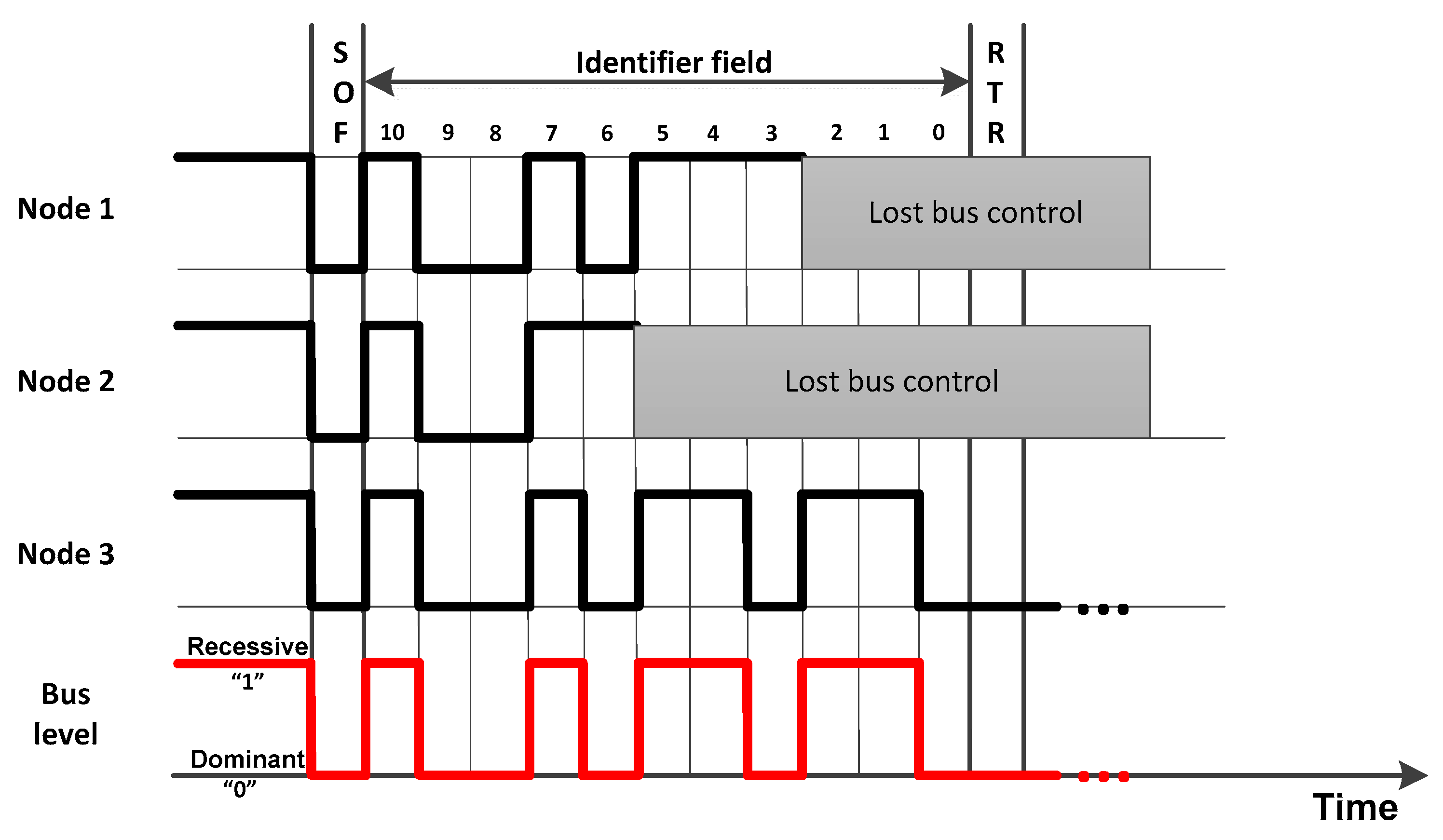
Similar to many other industrial wired protocols, the signals on the CAN bus is differential, which allows CAN to acquire its robust immunity to noise and fault tolerance. Differential signaling reduces the electromagnetic noise and allows a faster data rate over a twisted-pair cable. In particular, CAN uses a bit-wise arbitration mechanism to solve the collision problem. The Identification (ID) field of CAN message can represent both device information and message priority. The highest priority ID message always wins the bus access and keeps on transmitting when two or more devices start transmitting their message at the same time. An example to demonstrate this mechanism more clearly is shown in Figure 2. The CAN protocol includes five methods of error checking: two at the bit level and three at the message level. Due to all the reasons mentioned above, the total residual error probability of undetected corrupted messages is less than 4.7 × 10⁻¹¹, as mentioned in a previous study [31]. These characteristics make CAN one of the most reliable and popular protocols in industry, which is the reason for our choice of CAN in this proposed system.
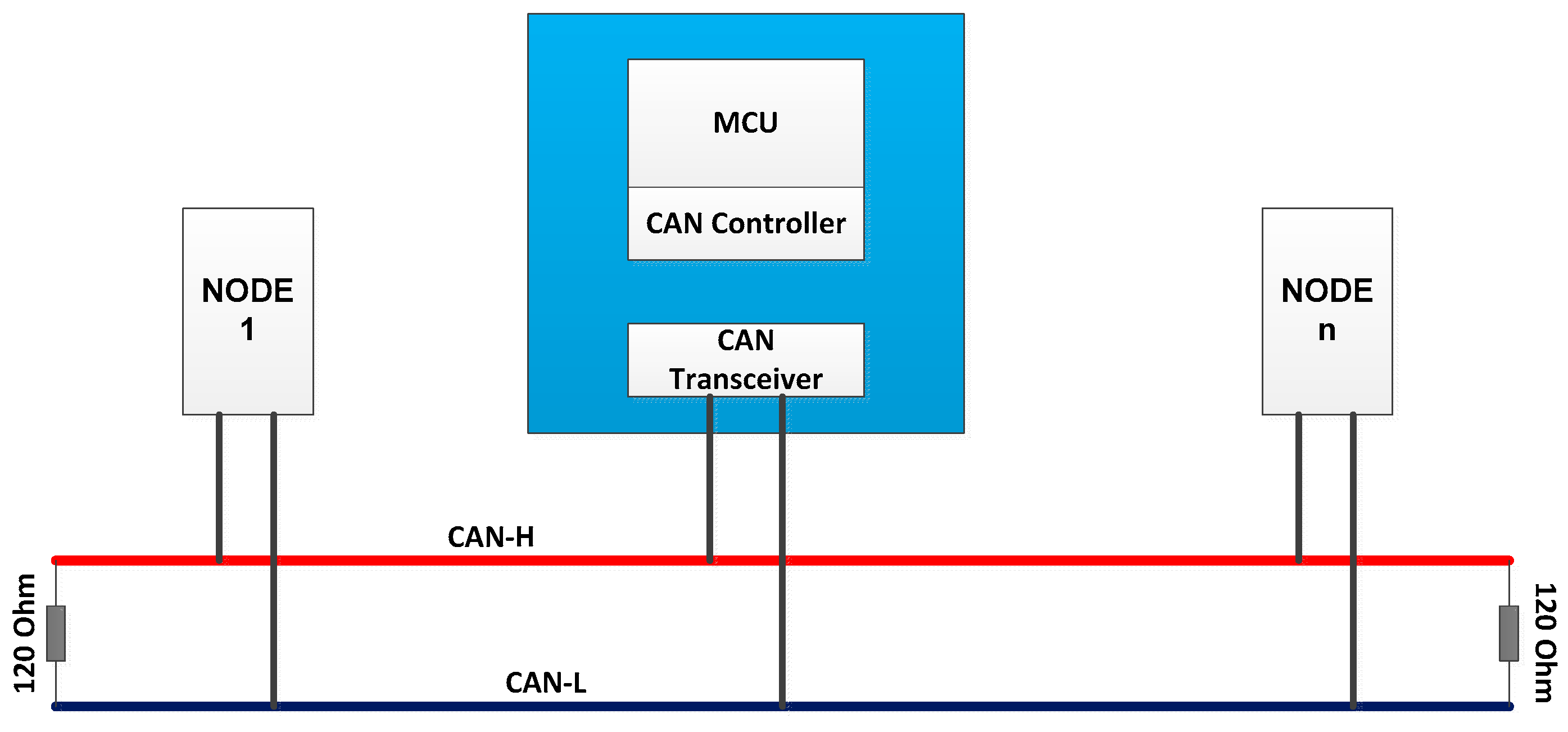
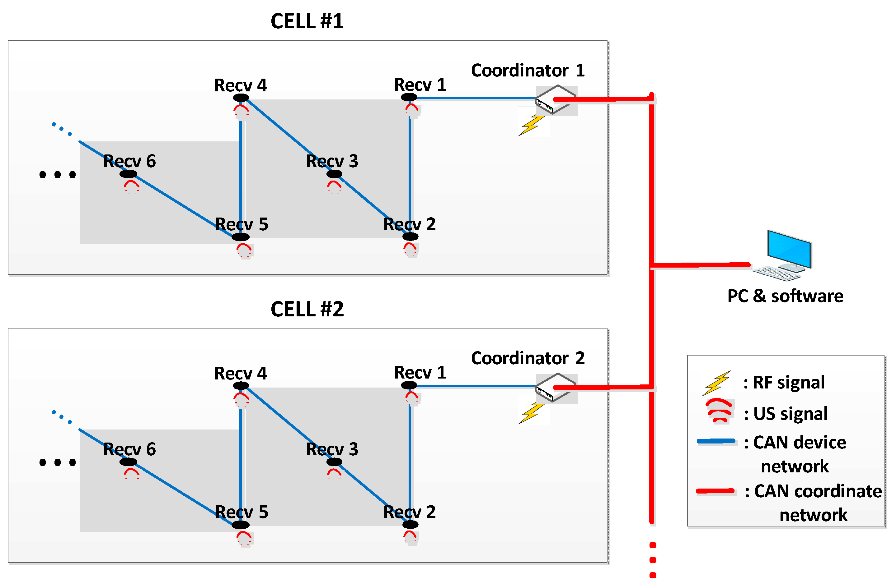
CAN replaces the complex wiring harness with a two-wire bus called CAN-H and CAN-L. Figure 3 represents a common CAN node/bus, as described by ISO-11898 [31,32]. This is also our system design, in which the coordinator and receivers talk to each other. This wiring simplifies our system installation and modification. Moreover, as stated above, CAN is a message-based protocol. It means there are many devices connected to the bus, with each device able to talk to one another. The CAN message is broadcasted in the network and devices can choose which one they want to accept by using a filter which is performed on the ID field of CAN message. This feature ensures the consistency of data in the network. Furthermore, this allows nodes to be added to or removed from the CAN network without requiring any change in the software or hardware of any other devices, even when system is operating (hot plug). This is the biggest advantage, which is comparable to other RF protocols, and allows our system to be easily extended in future studies. Extending the system can be chosen according to the scale of system by two ways: number of nodes in a cell or number of cells (Figure 4).
2.2. Design and Operation
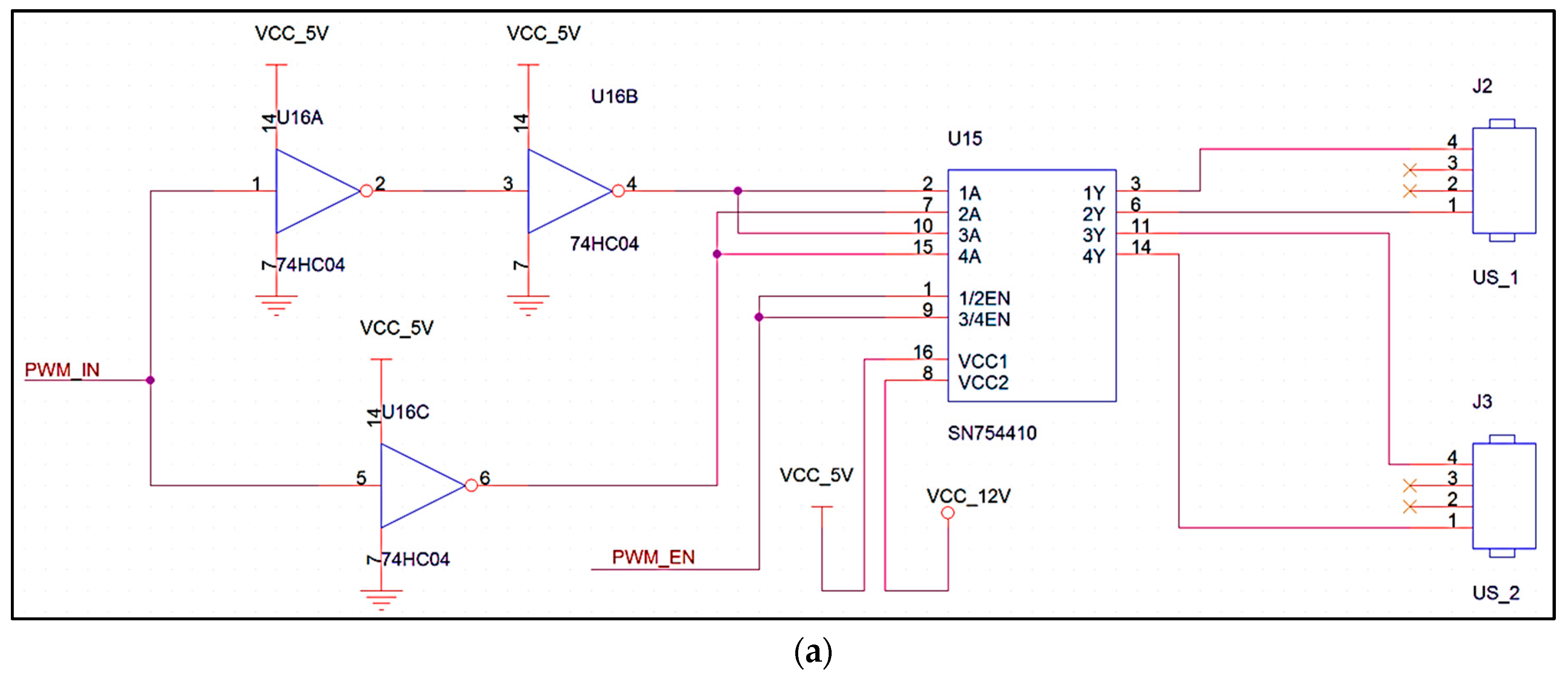
The transmitter device is equipped with a RF module for timing synchronization, a driver circuit and a transducer for generating an ultrasound signal. IC-SN754410 is used to boost transmission power. Combined with the IC-74HC14 Hex Inverting Schmitt Trigger, the voltage of the transducer is increased to 24 Vpeak-peak, which is the maximum value recommended in the specifications for the ultrasonic transmitter 400ST120. The main controller uses a Pulse-width Modulation (PWM) peripheral to generate a 40-kHz signal as an input for this driver circuit. The schematic of the ultrasound driver is shown in Figure 5a. The stack of a wireless protocol, which is called SimpliciTI (supported by Texas Instrument), is open source and is embedded on the main controller. This is a simple RF protocol, which supports the IC-CC110L sub-1 GHz RF transceiver. To put the system in operation, the transmitter needs to be attached on the target. At the beginning of each period, a RF signal is sent to indicate a trigger to receivers, resulting in multiple ultrasound waves being generated simultaneously. The emitting US pulse duration is 0.1 ms (about 4 wave cycles as shown in Figure 5b) and is managed by using a timer. The transmitter controls the sampling time of system by adjusting the RF–US transmitting duration. Currently, the maximum value of this period that ensures system functionality is at 20 ms or an updating rate of 50 Hz.
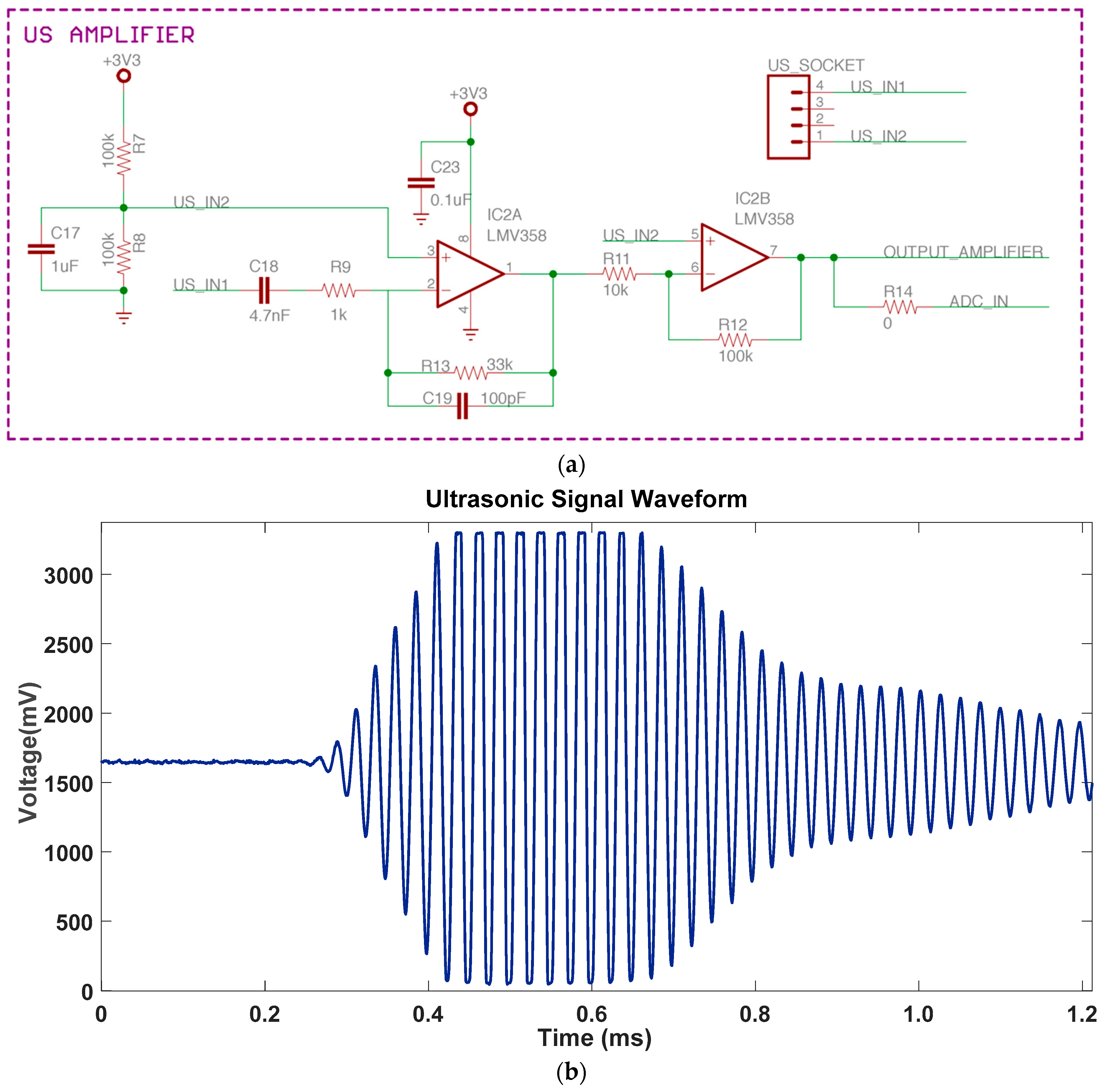
Receivers in our proposed system act as reference points, which receive and process US signals. Each receiver is composed of a transducer 400SR120, amplifier, filter circuit, CAN transceiver and main processor. After being received by the transducer, the US beacon is first filtered by using a band-pass filter comprised of Op-Amp as well as R and C components. This filter has a frequency center of around 40 kHz, which allows the desired frequency range and removes unwanted noise in other frequencies. This circuit also amplifies the US signal with a gain of 200 times. In the first version of our system, a threshold is applied to this pre-amplified signal using a comparator IC. The output of the comparator is used to indicate to the main processor that an US signal has arrived, which occurs in the form of a square wave. However, the arrival angle and long travel distance substantially affects the results. These factors can be diminished or even eliminated by using the sine wave detection method, which is proposed in Section 3.1. Fundamentally, the pre-processed signal is converted to a digital signal using the ADC peripheral. Following this, the sine wave detection method is applied to this digital signal in order to find out the exact time at which the US signal arrived. All receivers connect to the CAN network, which is coordinated by the coordinator device. This CAN network sends the TDoA information right after their processing procedure has been completed.
The coordinator in our system is responsible for managing all receivers. It also operates as a gateway between the PC and hardware system. The coordinator device includes a RF module (CC110L) and a CAN interface. This device receives a RF trigger signal from the transmitter device, generates a start message to all receivers and collects TDoA from all receivers via this CAN bus. Data exchange between these devices is based on a high-speed CAN protocol, which can reach up to 1 Mbps. After this, this information is transferred to PC via a serial interface.
Although the main processor of the coordinator device has adequate performance for processing, the trilateration algorithm temporarily performs on the PC software at the moment. This enables us to easily verify and change positioning methods. Moreover, a TCP/IP server is created to run in parallel with the positioning calculation. It publishes the target coordinate result to the other networks so that this information can be obtained from anywhere. It means that any client device connected to this network, including the target object, can use this information to carry out further positioning control techniques. There are two main advantages of using the TCP/IP network for such an application. First, it allows multiple clients to access the location data at the same time, which can be managed by the server. Secondly, TCP provides a reliable, real-time and error-checked data stream, so it can be used in any control system that requires a minimum chance for error.
3. Algorithms and Implementation
3.1. Sine Wave Detection Algorithm
The distance between the transmitter and the receiver is determined by measuring the time of flight of an ultrasonic wave. The ultrasound amplifier and band-pass filter circuit at the receiver node is shown in Figure 6a. In order to obtain an accurate result, the moment when the wave arrives at the receiver must be captured precisely. Since the ultrasound is a mechanical wave and the ultrasonic transducer at the receiver is used to convert the mechanical vibration into an electrical signal, the output signal requires a reasonable time in order to ramp up its amplitude. Therefore, when transmitting a 40-kHz ultrasonic wave, the received signal has the form of a sine wave with a central frequency of 40 kHz and a rising amplitude (Figure 6b).
A common approach for detecting ultrasonic waves involves the threshold mechanism. In this method, the amplitude of the receiver output is monitored continuously. The moment this amplitude reaches a pre-configured DC voltage value is considered as the time of arrival of the wave. This method is easy to set up as it only requires a comparator circuit to detect a threshold voltage without any processing power. When the ultrasound arrives at the receiver, the sine wave amplitude will gradually increase. When this amplitude exceeds the voltage threshold, the comparator will trigger the distance calculation process.
The above method was used in the first version of SNSH localization system. This showed that the accuracy of this approach is determined by choosing a proper threshold value. A small threshold allows us to detect the presence of an ultrasonic wave faster, but it is also more susceptible in detecting wrong pulses from the echoed wave and random noise from the circuit. On the other hand, a larger threshold value is more resilient to circuit noise and echoed waves, but it requires the wave to ramp up its amplitude for a few wave cycles before it can be reached. Therefore, the calculated distance with a large threshold is usually greater than the actual distance. As a result, this threshold detection approach only works well when the received wave is strong and rises up quickly. Specifically, this needs a short distance and a narrow angle between the transmitter and receiver.
To better identify the arrival of an ultrasonic wave at the receiver, the detector should be able to recognize the presence of a wave pulse at a small amplitude. In this paper, a sine wave detection algorithm is proposed to address the drawbacks of the threshold detection method. The theory of this new method involves creating a local copy of waveform with similar characteristics of the wave that need to be recognized, before correlating it with the incoming wave [33]. The correlation is conducted by multiplying the incoming signal with the local copy sample by sample for a detection duration time of T, before integrating the calculated results. If the two signals are similar, multiplying them is basically the same as squaring the incoming wave. Integrating the results for a time duration will generate a large number. On the other hand, if the incoming wave is different from the local waveform, the multiplying process will produce negative values and integrating these values would result in a smaller value.
Let the incoming wave be formed as follows:
where is the incoming sinusoidal wave frequency; θ is the initial phase; and A is wave amplitude. This initial phase is an important factor because the received wave is not always in the phase with the local replica. Following this, let the local copy waveform with a frequency f be:
Mathematically, the detector calculates the integral in a period T = 1/, which is given by:
Suppose that the incoming wave and the local copy share the same frequency, f = , we obtain:
Solve the integral above, before the output of the detector is determined as:
As we can see, the integral result depends on the initial phase θ of the incoming wave. When θ = 90°, the detector output will be zero although the incoming wave and the local replica share the same frequency. To handle this situation, the incoming wave will be multiplied with a second local copy, which is 90° out of phase with the first copy. Specifically, the second local waveform and its integrating result will be:
Let T = 1/ (a period of a 40-kHz sine wave signal) and substitute into Equations (5) and (7), we have:
Therefore, we can find that:
Furthermore, the average power of a sine wave with an amplitude A within a period T = 1/ can be calculated by:
In conclusion, the result of S is independent of the phase difference between the incoming signal and local copy. Moreover, the output of the sine wave detector will be basically proportional to the power of sine wave only when both of these signals have the same frequency. Essentially, a larger difference in frequency decreases the magnitude of S. Thus, the detector also operates as a filter in eliminating the effect of noise.
3.2. Implementation and Simulation Result
As mentioned above, the sine wave detection algorithm can be considered as a new technique to detect the arrival of the incoming wave by measuring the power of ultrasonic waves at the receiver. The fundamental procedure involves first sampling the output signal of the receiver continuously at a constant sampling frequency, before using the sine wave detection algorithm at the end of each wave cycle. The output of the wave detector, which is proportional to the wave energy, will be used to determine the existence of an ultrasonic wave. As the wave detector only responds to waves at 40 kHz, its output is not influenced by random noise and is more sensitive to ultrasonic waves with smaller amplitude.
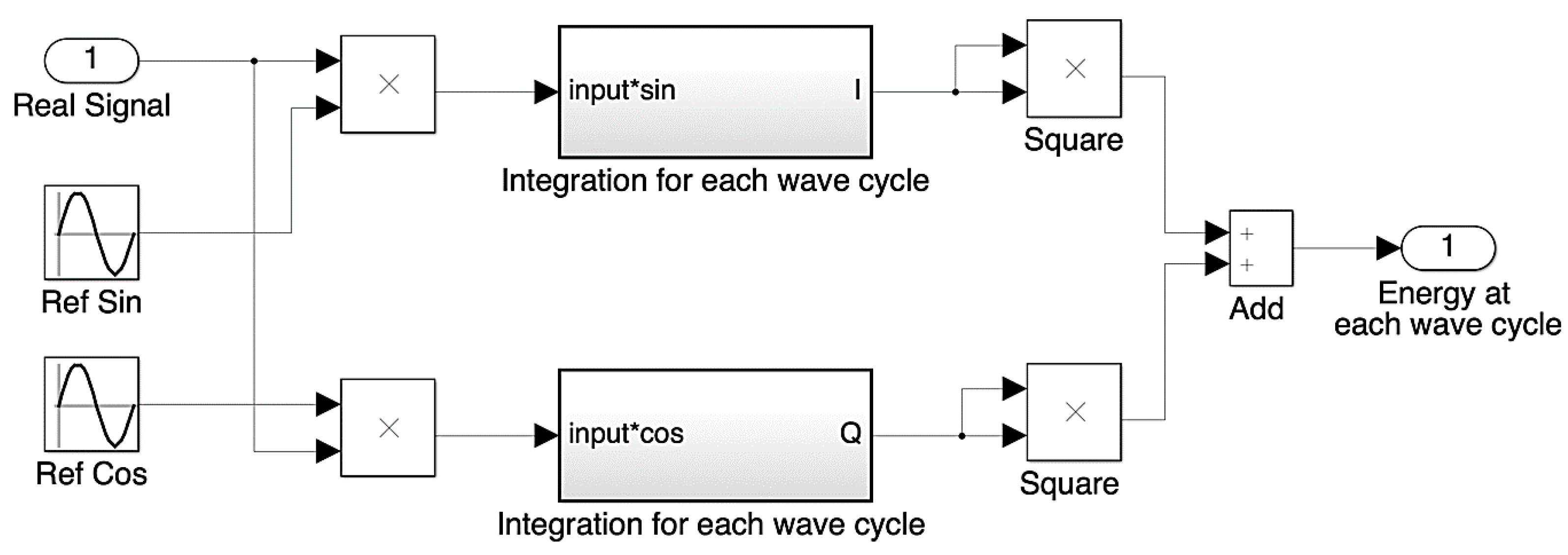
A MATLAB simulation model has been designed to demonstrate the performance of the wave detector as shown in Figure 7. In theory, the ultrasonic waveform is a continuous time signal and the detector must run two integral calculations to achieve the result. However, this method is not applicable to digital processing, where the wave is sampled at constant frequency and calculation is applied to an array of samples. Therefore, the MATLAB modelling will be constructed in the discrete time domain, where sampling frequency plays an important role in the system.
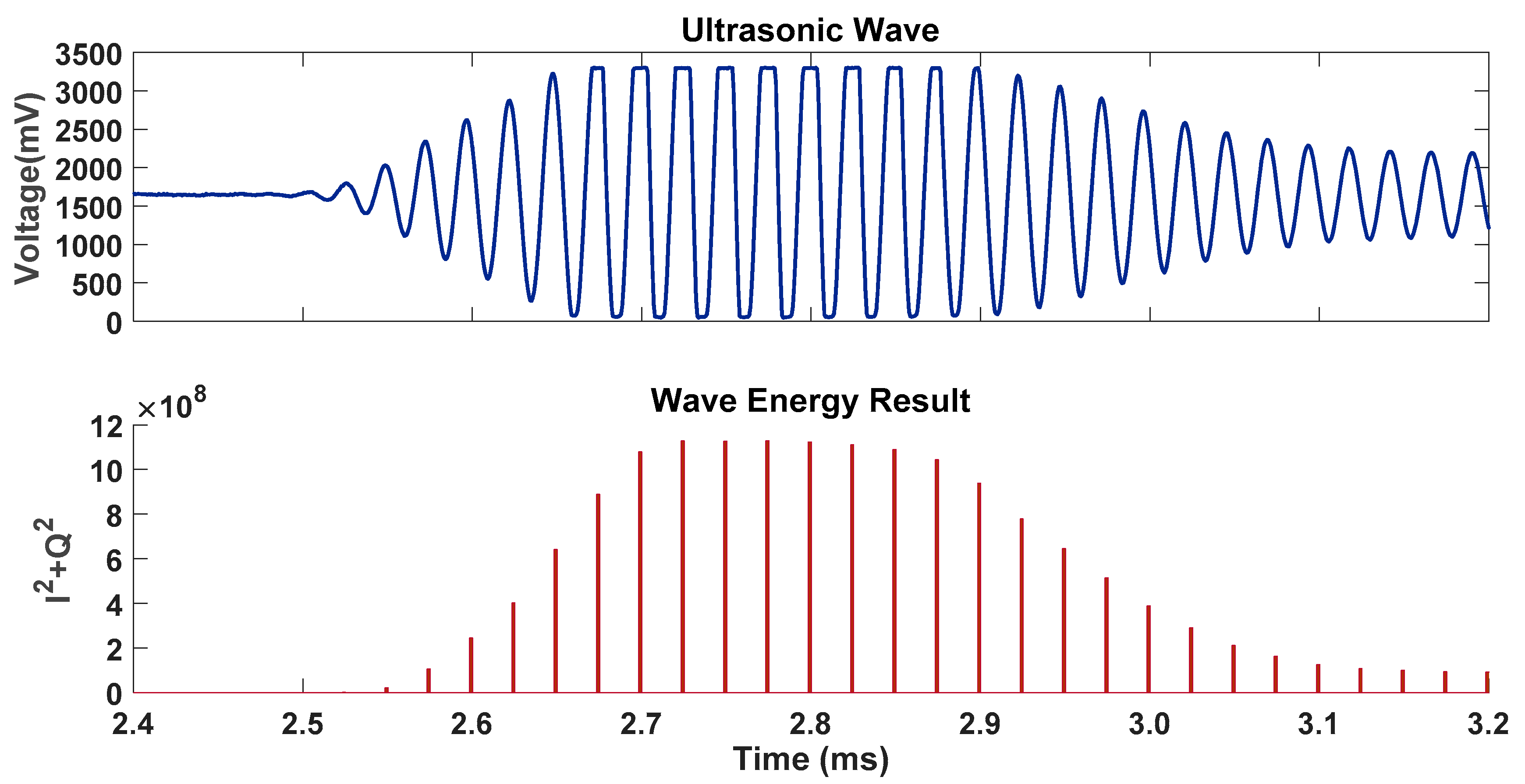
The modeling system consists of two components: a sample of the ultrasonic wave and a wave detector. First, the ultrasonic wave sample is obtained by ADC conversion at the receiver output. The digital buffer is then stored in a text file and imported into MATLAB as an array. Secondly, a wave detector is established by applying the detector theory in the discrete time domain. Two local copies of the 40-kHz sine wave are created, which are specifically called and , where = 40 kHz (frequency of the ultrasonic signal). Following this, a detector of duration period T is chosen as one wave cycle, which is T = 1/. After this, the output of the detector will be calculated as described in the detector theory and the integral function will be replaced by the adding function in the discrete time domain. Simulation result of sine wave detector using real wave signal is shown in Figure 8.
In conclusion, the simulation model demonstrates that the proposed wave detector is very effective. The output result is proportional to the squared amplitude of the sine wave and is independent of the initial phase, so it is easy to detect the presence of ultrasonic waves at a very small amplitude without being affected by random noises. Moreover, this method does not require too many calculations and provides results at each wave cycle. In comparison, the correlation algorithm applied in previous studies [22,23] have to re-calculate the correlation coefficient of the wave sample sequence. Along with the high-performance operation of micro-controller unit (MCU), this detector is easily embedded into the receiver board.
3.3. Least Square Problem
The classical approach of the 3D positioning problem considers the intersection point of spheres whose centers are the locations of reference points Ri(xi, yi, zi) as target coordinates T(x, y, z), which are defined as:
where di is an exact distance from target to reference point i. Solving n non-linear equations provides us with the coordinates for the point of intersection. However, this procedure requires a long computing time and significant resources due to the complexity of equations. Additionally, the equations are quadratic, which usually have two roots or more that need to be considered and verified.
Simultaneously linearizing equations converts this problem into an easier problem is to solve a set of linear equations. This helps us to reduce the number of required calculations and simplify the procedure. Inserting point Rj(xj, yj, zj) into Equation (12) provides:
Expanding and grouping this again leads to:
where i, j = 1, 2, …, n is the number of beacons; while di, dj and dij are the distances between the target and beacon i, j as well as the distance between the two beacons i and j, respectively. When this is rewritten in matrix form, it becomes the following:
where:
The problem is converted into finding the intersection of planes, which is a simpler problem than the original. However, for n beacons, the system of Equation (15) has (n − 1) equations in three unknown variables. Theoretically, only four beacons (n = 4) are needed to determine the unique points of the target in order to correctly measure distance.
In fact, the distances between these beacons and the target cannot be determined exactly as measurement noise causes incorrect information to be relayed and requires us to have more than 4 receivers to increase accuracy. The range of the measurements is formed as calculated in Equation (16):
where ri and εi are approximated distance of the target from the beacon i-th and measurement noise, respectively. The results for the distance follows a normally distributed population (Gaussian), with measurement noise being considered as the variance of this measurement. The location problem is therefore solved by using the least square method, which is discussed clearly below.
The Least Squares algorithm defines an objective function or cost function, which is the sum of the squared residual value, and optimizes system accuracy by determining x* to minimize this function.
A necessary condition for the local minimizer is that x* must be a stationary point of F or equivalent to solve the gradient equation, with an adequate condition being a positive, definitive Hessian matrix F”(x*).
Usually, F(x) is rewritten in the matrix form as follows:
For the system of linear equations in Equation (15), this is a linear least square problem in which function f is formed as:
Thus, x* is the solution of normal equations and is obtained as follows:
Certainly, the general method for solving the least square problem is to find the x* that satisfies both the necessary and sufficient condition. However, it is very hard to solve this problem completely in general and it is not an effective way. The Nonlinear Least Squares (NLS) method presents another solution, which solves the simpler problem of finding a local minimizer inside a certain region whose size is given by a small positive number δ. The NLS problem can be summarized in this case as follows:
Furthermore, for developing the embedded system, it is necessary to establish a common approach, which can be realized by the programming language on PC. Accordingly, the iterative methods for non-linear optimization are carried out according to the procedure in Algorithm 1 below. From a given point x(0), the program calculates a series of x(1), x(2), …, x(k), x(k + 1), which satisfies the descending condition and converges to the local minimizer, x*.
| Algorithm 1: Pseudo code for C implementation of general NLS method |
| do { k = k + 1; x(k) = x(k−1) + Δx; if (F( x(k) ) > F( x(k−1) ) ) break; } while (k < kmax) |
Several different approaches can be taken: Gauss–Newton, Levenberg–Marquardt, Powell’s Dog Leg or hybrid methods, which combine modifications of these methods. In this paper, we present the Gauss–Newton method with a best initial value x(0) obtained from LLS method, which was discussed above. This method is based on the implementation of the first derivatives of the function. Therefore, it is very basic and numerically efficient because the second derivatives that can be challenging to compute are not required.
First, F(x) is chosen as the sum of the squares of the errors for the distances as stated earlier in Equation (22):·
Generally, with a small h, the Taylor expansion of every function around x is defined as:
where J(x) is Jacobian matrix or gradient of F(x), which contains the first partial derivatives of (x).
Equations (23) and (24) lead to:
The Gauss–Newton step hgn is chosen to minimize F(x + h). Therefore, the necessary condition and sufficient condition must be satisfied for F(x + h).
Let A = JTJ and AT = A, which allows A to be symmetric. As demonstrated in a previous study [28], if J is linearly independent and has a full rank, this leads to A being positive and definite. It also shows that F(x+h) has a unique minimizer, which can be found by solving:
In this case, JTJ and JTf are defined as follows:
Thus, the Gauss–Newton iterative method is now derived as follows (Algorithm 2). The stop condition can be a threshold of the error or the maximum number of steps.
| Algorithm 2: Pseudo code for C implementation of Gauss–Newton iterative method. |
| do { k = k + 1; if (J is full rank) { x(k) = x(k−1) + hgn; delta = F( x(k−1) ) − F( x(k) ); } else { break; } } while ((delta > threshold) && (k < kmax)) |
3.4. Implementation and Simulation Results
This section presents the MATLAB program used to simulate the operation of two proposed methods. The output results are also used for comparison with other studies as well as comparisons with one another. The realization from MATLAB shows that LLS and NLS is not complex and they can be fully implemented by any language, such as C, C++ or by C# in our project. The simulation program includes two parts.
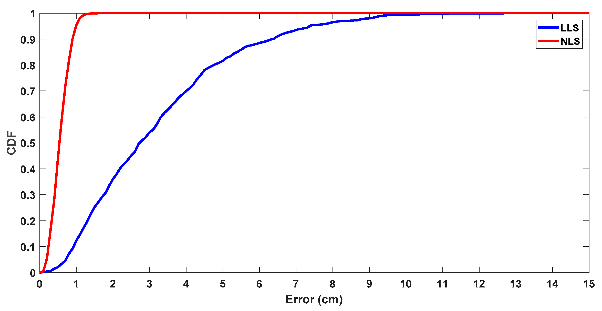
At first, N random points are generated so that they belong to the workspace of the system. Distances from these points to the pre-defined reference nodes are also derived. External disturbance or measurement noise is presented by a random value and it will be added to measurement results. The variance of noise shows the maximum measurement error or the accuracy of distance measurement. These results for distance after adding noise will be under the trilateration process for retrieving the target coordinates in the second step. Indeed, these coordinates will be different to the original ones. The accuracy of algorithms is determined by finding out the deviation. Cumulative distribution function (CDF) of the Euclid distance error from simulation result is shown in Figure 9. This procedure is summarized as shown in Algorithm 3:
| Algorithm 3: Pseudo code for MATLAB implementation of generating test data and evaluation of their errors |
| for i = 1 to N original_point(i) = random(1, 2) * workspace_dimension; for j = 1 to k dij(j) = distance(original_point (i), reference_node(j) ); end estimated_point_LLS(i) = Linear_least_squares(reference_node, dij); estimated_point_NLS(i) = Nonlinear_least_squares(reference_node, dij); error_LLS(i) = distance(estimated_point_LLS(i), original_point(i) ); error_NLS(i) = distance(estimated_point_NLS(i), original_point(i) ); end |
4. Experimental Results
This section presents our proposed method for the experiments. Each approach is implemented in real hardware and software, before data is collected to evaluate their performance and practicability.
4.1. Sine Wave Detector
Modern micro-controller unit (MCU) offers high-performance computing solutions for embedded systems where reliability, high availability and real-time responses are needed. It also supports connectivity protocols and other features at a low cost. It provides a standard industrial protocol CAN version 2.0 A/B. It has Direct Memory Access (DMA), a great feature of the microcontroller system, which allows peripheral units to transfer data directly to or from memory without being handled by the processor. Thus, it is perfectly suitable for dealing with a large stream of data from the ADC peripheral with minimum delay in between. It has a higher efficiency than an interrupted routine, which requires the processor to manage data at each interrupted event. The Floating Point Unit (FPU) is a part of the system designed to handle fast calculation of float numbers and to be a power-efficient algorithm of digital signal control applications, such as sensor fusion, motor control and power management. These three factors work together to enable a single chip solution, which reduces module size, increases cost efficiency and enables system scalability. In our experiments, an ARM Cortex M4-based MCU STM32F4 is chosen as the main processor of receiver node.
According to the system configuration, the transmitter will first transmit a pulse of ultrasonic wave after sending a RF signal. Following this, the coordinator will wait for a RF trigger signal to initiate distance measurement procedure in all receiver nodes. Each receiver node will receive a broadcasted start message on the CAN bus, which is sent from the coordinator, to start distance measurement process. Following this, three stages will run in sequence to determine the initial wave cycle: ADC conversion, sine wave detection algorithm and dynamic threshold filter (Figure 10).
First, the processor starts the ADC conversion of US receiver output signal after triggered by a start message from CAN bus. The conversion will run continuously in a sampling duration T, with a fixed sampling frequency of 1.4 Mega-Samples Per Second (MSPS). The sampling duration is chosen so that the receiver can capture the incoming wave at the longest distance in the workspace. For example, assuming that the maximum distance is 5 m, the sampling duration T is calculated as follows:
In the second stage, the discrete wave data are split into small buffers, with each one storing the information of one ultrasonic wave cycle. These small buffers form the inputs of the sine wave detection algorithm. After calculation, the output of the detector is the wave energy at 40 kHz for each wave cycle. Following this, these energy results will be passed to a dynamic threshold filter in the third stage.
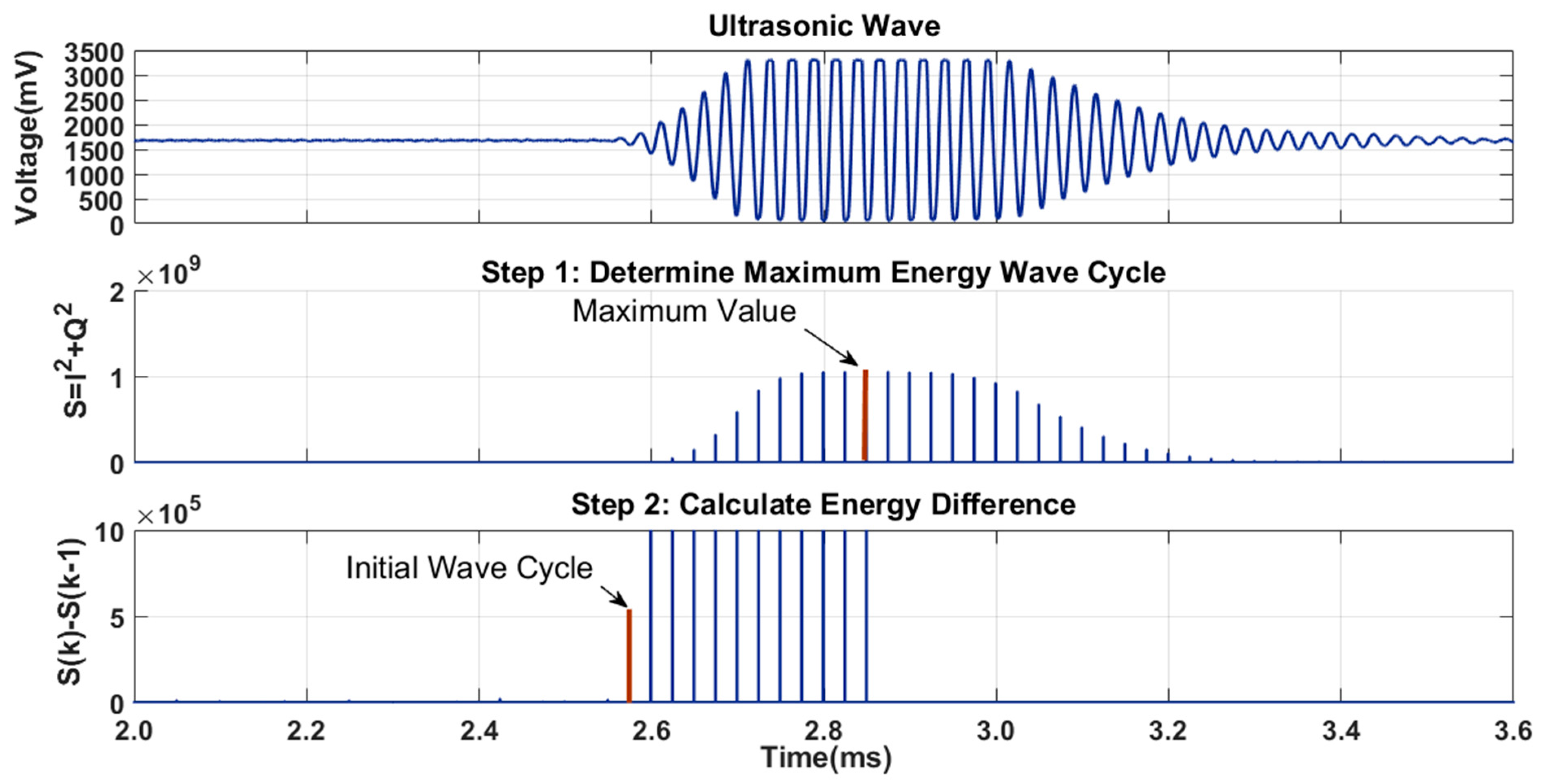
This digital filter is designed to eliminate the effect of the echo wave and circuit noise. In theory, the first beam that arrived at the receiver is the wave that was sent directly from the transmitter and has the biggest amplitude. This is followed by several echo waves with smaller amplitudes. Therefore, by spotting the wave cycle with maximum energy, the direct wave is pinpointed and separated from the echo waves. In addition, as the maximum energy is resolved by bubble sorting energy data at each trigger cycle, this value is dynamic and unaffected by the range of measurement and transmitting angle, which decides the amplitude of the incoming wave. Following this, the wave cycle with a maximum energy value is chosen as a starting point for the second step. The energy difference between the current cycle and the previous one is calculated repeatedly, starting from the detected maximum cycle back to the start of the buffer. The loop stops when a minimum threshold of energy difference is passed for the first time and the current cycle is chosen as the starting point of ultrasonic waves. Results of the dynamic threshold filter with real wave signal are shown in Figure 11. Finally, the time of flight is obtained by a calibration process to give a precise relationship between the initial wave cycle as well as the distance between the transmitter and the receiver.
Ideally, the measurement time includes a US flight time of maximum range and mathematical processing duration, which is about more than 15 ms for a 5-meter range. However, there are also many disturbance factors added to this period, such as the delay in time for encoding/decoding RF messages, CAN sending and receiving packets, reflection effects of US wave at receiver nodes, etc. Therefore, to reach the maximum performance of our system, the operation period is evaluated and reduced by experiments. At our laboratory conditions, the system operates steadily with a precision of under 1 cm at an updating rate of 20 ms. All the data about the measured time will be available at the server after around 22 ms, which includes the time needed for transfer by CAN.
As previously discussed, the measurement time is composed of a constant delay. Thus, the relationship between the distance d and corresponding time difference of arrival Δt is given as follows:
where v (slope) is the ultrasound speed (theoretically, v ≈ 340 m/s) and c (offset) is a constant.
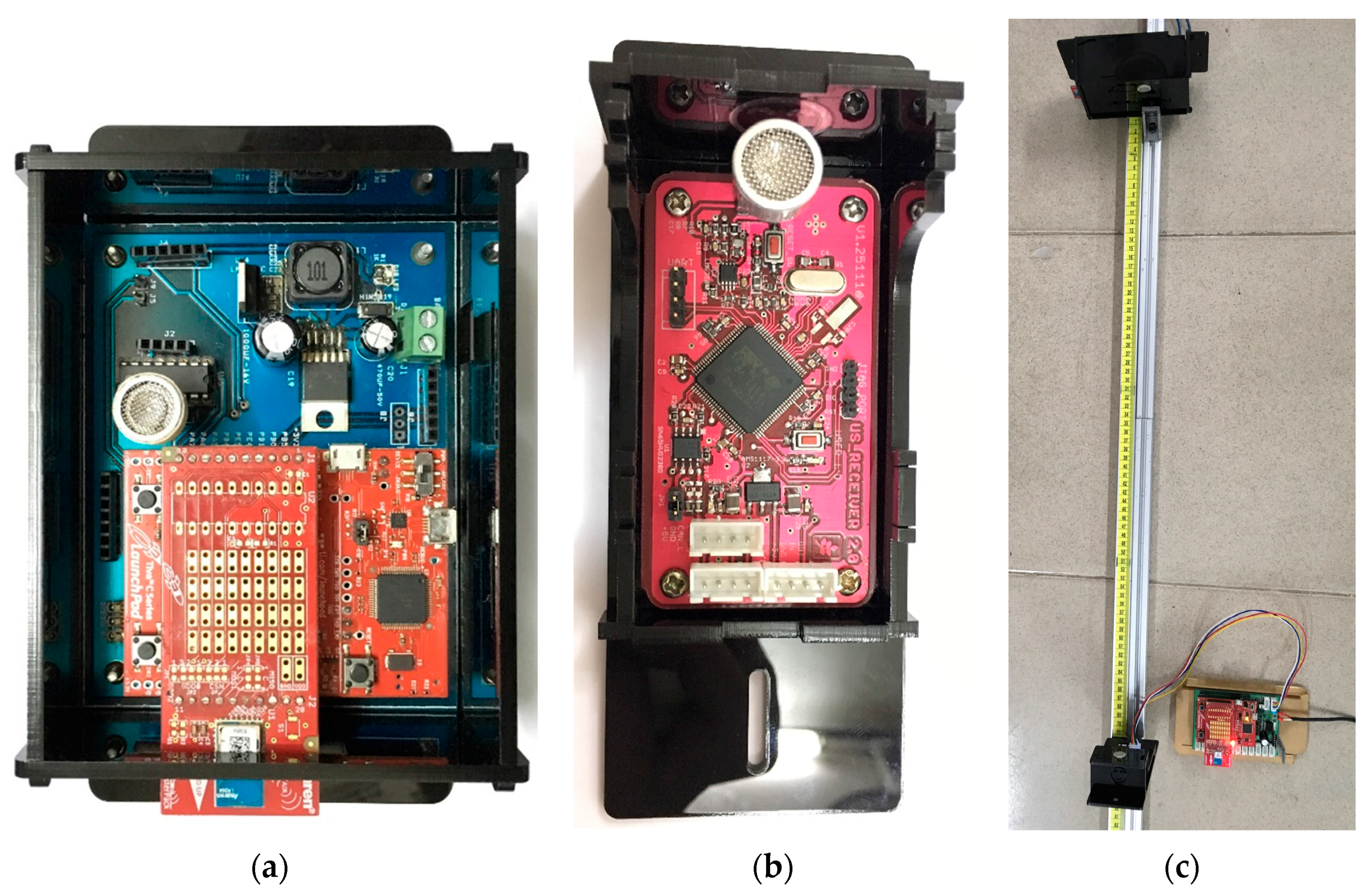
In this paper, to figure out the exact estimation for Equation (30), the calibration phase has to be conducted before putting in use. The receiver is considered as a stationary point, while transmitter is moved around with changes in distance and angle of arrival (Figure 12). Through this calibration, Equation (30) and average error for the distance measurement can be resolved. The experimental results and comparison with other researches are shown in Table 1.
An example for this relationship on a receiver node is presented in Equation (30). ·
Theoretically, the sine wave detector method involves a possible error in the time measurement of a period (of the 40-kHz ultrasound signal), which is approximately a distance of 8.6 mm.
4.2. Least Square Algorithms
After the measurement phase has determined the distances to all reference nodes, the coordinates of the object are retrieved using the Least Square methods. The hardware setup and implementation of the second phase is realized as follows.
The coordinates of reference nodes are calibrated and fixed at pre-configuration points (Figure 1). In our experiments, five reference nodes are mounted with their coordinates listed in Table 2.
In addition, to ensure that the distance measurement error remains under 1 cm, the test points are chosen so that they satisfy the condition as mentioned previously in Section 4.1. This condition is that the angle of arrival remains under 45°. The transmitter has to be settled inside the workspace (Figure 1).
Finally, in our experiments, the transmitter is a static object, which maintains its position during measurements and data processing. The approximate distances of the transmitter to the reference nodes are available after finishing the first phase. In the second phase, Least Square Estimation methods are implemented in C# language and Windows platform using the results from the first phase. After the target coordinates are determined by applying the LLS and NLS methods, the positioning results are recorded along with the approximate distances in the text file. Short descriptions of these two steps are presented in the flowchart in Figure 13.
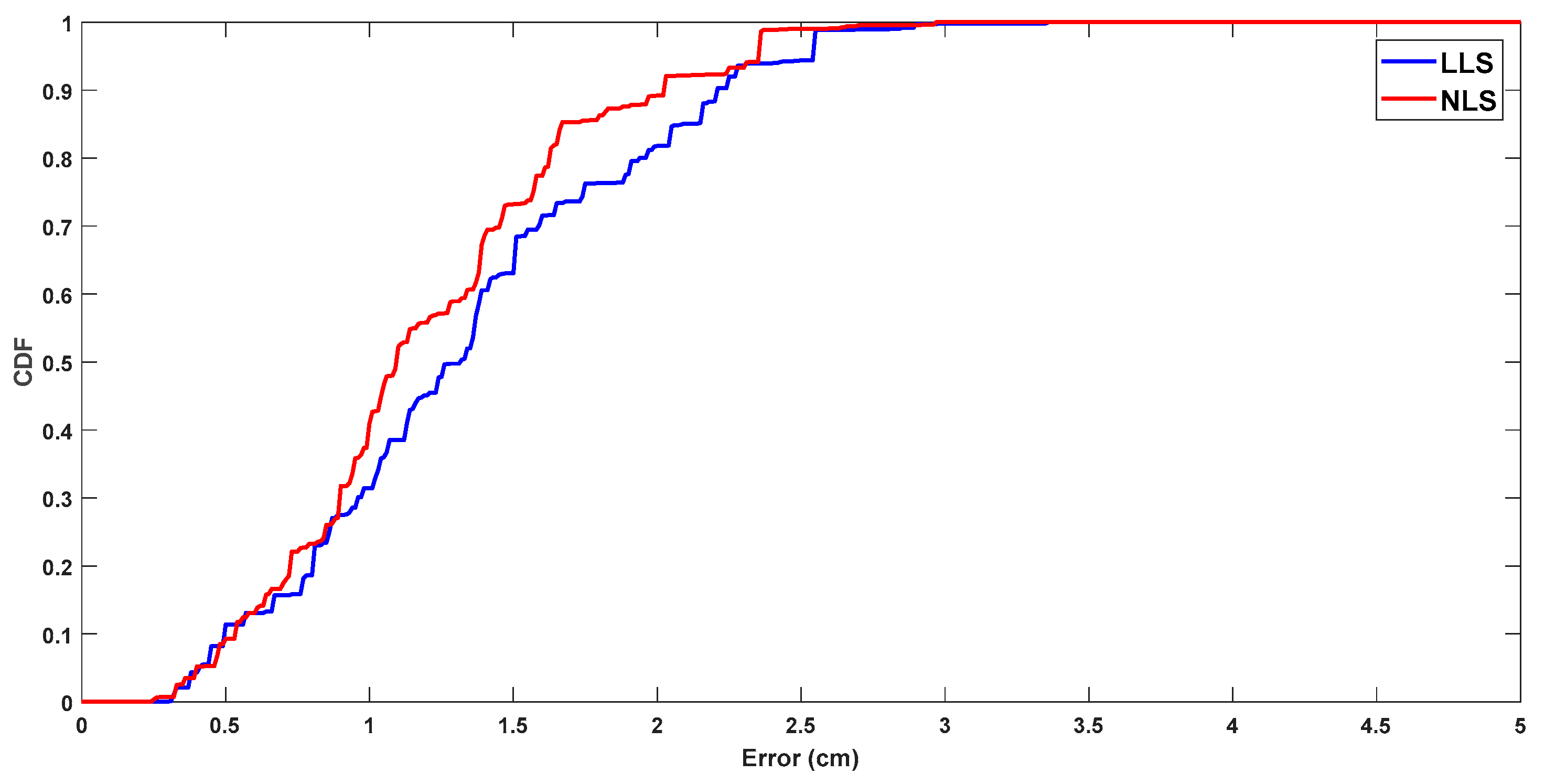
The true positions and calculated points determined using the Least Square methods are compared to illustrate the effectiveness of the algorithms. The evaluation is shown in Figure 14 and Table 3.
In brief, NLS certainly achieves a higher accuracy than LLS. The cost function of NLS describes exactly the error which the user needs to optimize. At the same time, LLS’s cost function is figured out after linearization as:
The target point needing to be addressed in the LLS method is (x−xj, y−yj, z−zj), while the cost function includes more measurement numbers (di and dj). Therefore, the error is amplified and higher than NLS. In comparison, the realization of LLS is considerably simpler than NLS and requires less math operators, especially matrix multiplying and inversing. The cost function does not have to be calculated repeatedly in each step in the iteration as NLS. Fortunately, the performance and resource of modern embedded systems are constantly increasing so they can perform more sophisticated functions compared to the past. Accordingly, there are no significant problems for implementing NLS on a microcontroller, such as STM32F4 in our system.
As mentioned previously, the distance measurement period is 22 ms. After the range estimation data is available at PC, LLS and NLS requires about 3 ms to resolve the location problem and produce the coordinates of the target. The experiments show that 25 ms is the minimum value for a stable operation. Table 4 shows the comparison to other completed indoor localization systems.
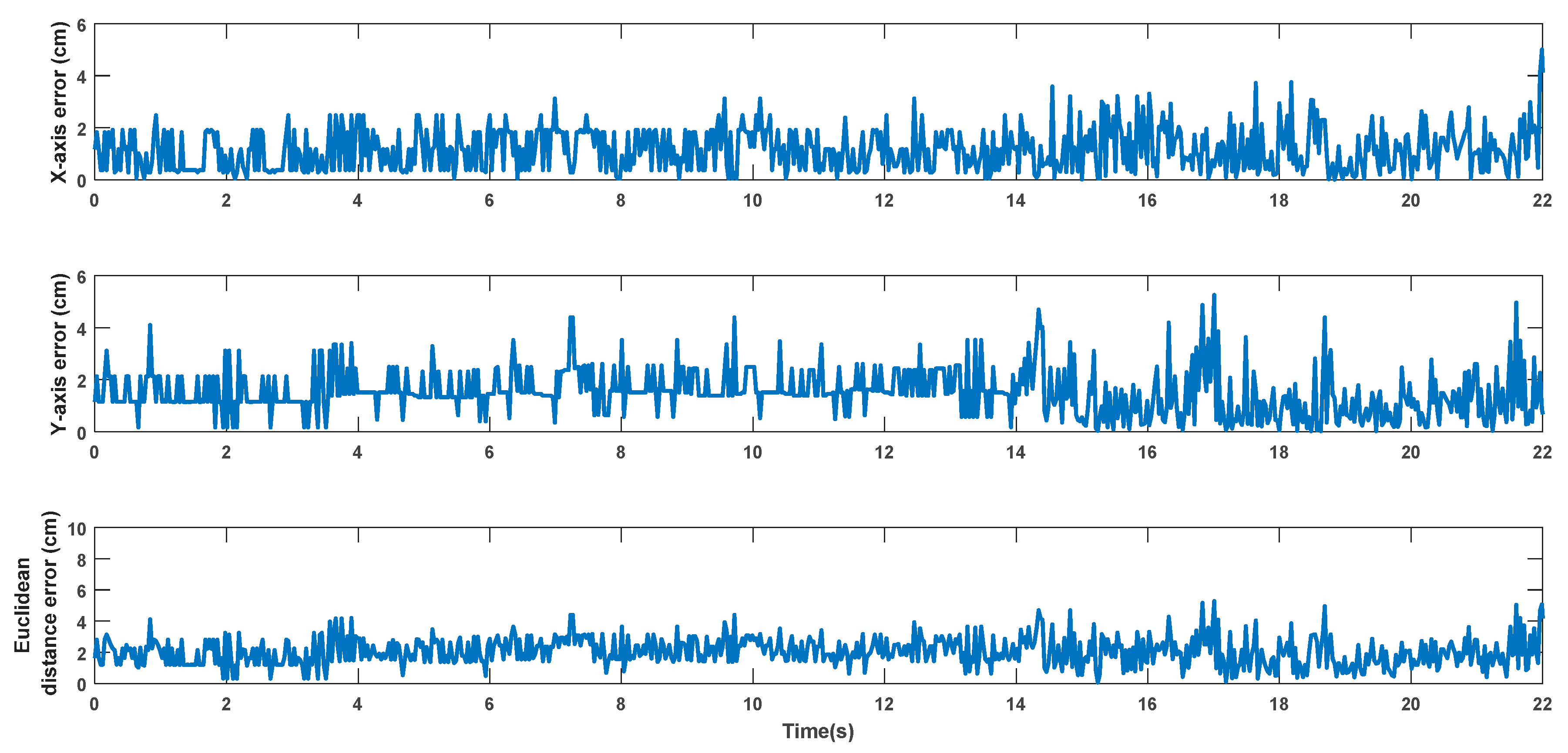
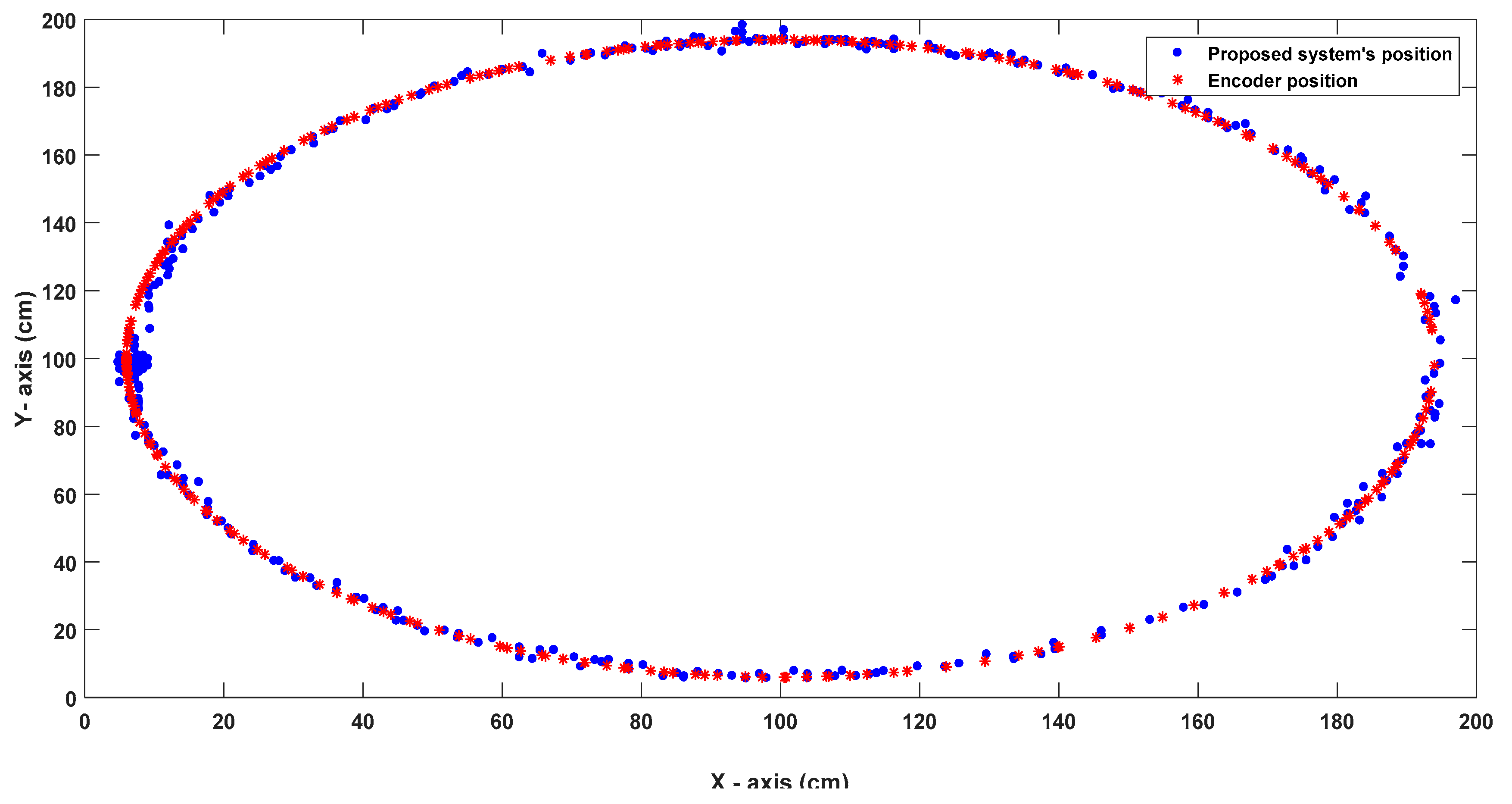
Certainly, the obstacles can seriously affect the accuracy of system due to the reflecting effect or even the disturbance from the ultrasonic signals. On the transmitter side, only 4 cycles of the ultrasound are sent so that there are not too many ultrasonic signals in our system. The period of 25 ms is also long enough for the direct wave signal and a 1-time reflected signal to move out of the next localization cycle. In addition, the dynamic threshold filter is applied to distinguish the direct wave signal, which has the greatest amplitude, from the echo wave with a significantly smaller size. Ultrasound-based localization systems are also affected by the Doppler effect in the case where the targets are moving objects. To verify the system performance in these situations, we have carried out another experiment with moving targets (approximate 2 rad/s), which is attached to a turntable with 1 degree of freedom using a high-resolution rotary encoder (2000 ppr) as shown in Figure 15. The results of the dynamic test are shown in Figure 16 and Figure 17, which demonstrates the decline in accuracy due to the Doppler effect. This problem is common among the ultrasound-based localization systems and can be further enhanced by adding additional motion sensor sources, such as camera vision or Inertial Measurement Unit (INS).
5. Conclusions
Various distance measurement techniques in an ultrasonic-based localization system have been developed and can produce highly accurate results. In this paper, an innovative approach for detecting the arrival of ultrasonic waves has been investigated using a sine wave detector. Its implementation contributes another way to determine the distance between two moving points using the TDoA technique based on ultrasonic and RF signals. Compared with other mechanisms, the range analysis using a sine wave detector offers higher accuracy compared to conventional threshold methods. Furthermore, this has an accuracy that is similar to the correlation technique, which generally remains below 1 cm. Also, it takes less time to perform a completed algorithm and it does not repeat the calculation for each sample, such as in the correlation mechanism. Therefore, it can be embedded into the main board and operates in real-time as a stand-alone unit. The accuracy and updating rate are verified and mentioned clearly in real deployment. However, due to the effective beam angle constraint of the ultrasonic transmitter, the proposed method only works well at a maximum angle of arrival at 45°. For this reason, the position of the target needs to be restricted in a workspace that satisfies this condition.
Additionally, the real indoor localization system called SNSH has been carried out based on range analysis using multilateration algorithms. CAN network, which shows prominent characteristics as discussed in Section 2, serves as a communication protocol between the coordinator and a number of reference nodes. The proposed hardware system demonstrates a high reliability for data transfer as well as ease in installation, operation and maintenance process. In particular, the system can be extended and upgraded up to (211-1) reference nodes based on addressing the CAN protocol without a change in the hardware structure, which only requires minor steps for updating the information from the new nodes in the software. Two multilateration algorithms, LLS and NLS, are applied and experimented in the SNSH localization system to find the optimal 3D position from distance measurement results. In our final system deployment, the average error in position remains under 15 mm, with 90% confidence error values of about 23 mm for LLS and 20 mm for NLS. Increasing the updating rate of system is also our contribution. The arriving signal is considered in settling time to minimize the algorithm calculating duration instead of modulation/demodulation. This helps us to reach a faster updating rate of up to 40 Hz, which is better than many other studies. A short comparison between the SNSH system and previous indoor localization architectures concludes this paper in Table 3 and Table 4.
Our long-term goal is to build fully stand-alone system with a main board running on Linux, along with easily configurable software and devices because current localization algorithms run on PC and cannot adjust reference node coordinates seamlessly (only by hard-coding). Furthermore, the CAN network can be utilized for other purposes. Its bandwidth is sufficient to handle other data streams, such as sensor acquisition or remote control. On the other hand, the system period or sampling time can be further reduced since the modern MCU has increased processing speed and can perform complex digital signal processing in a short period of time. Most of the highly accurate localization systems are under evaluation for verifying algorithms and are only designed for laboratory experiments. In this paper, we presented a completed solution for the indoor positioning problem, which includes the two phases for measurement and localization, and released a fully functional evaluation system for this purpose.
Acknowledgments
This work was supported by Ho Chi Minh city University of Technology (HCMUT), funded by Vietnam National University—Ho Chi Minh city (VNU-HCM) in the project C2015-20-05.
Author Contributions
Tan-Sy Nguyen and Thai-Hoang Huynh conceived and designed system architecture; Tan-Sy Nguyen and Trong-Nghia Nguyen analyzed and developed algorithms; Quoc-Sang Tran and Trong-Nghia Nguyen implemented algorithms; Tan-Sy Nguyen, Quoc-Sang Tran and Trong-Nghia Nguyen implemented hardware and performed the experiments; Tan-Sy Nguyen, Trong-Nghia Nguyen and Thai-Hoang Huynh wrote the paper.
Conflicts of Interest
The authors declare no conflict of interest.
References
- Liu, H.; Darabi, H.; Banerjee, P.; Liu, J. Survey of Wireless Indoor Positioning Techniques and Systems. IEEE Trans. Syst. Man Cybern. Part C 2007, 37, 1067–1080. [Google Scholar] [CrossRef]
- Gu, Y.; Lo, A.; Niemegeers, I. A Survey of Indoor Positioning Systems for Wireless Personal Networks. IEEE Commun. Surv. Tutor. 2009, 11, 13–32. [Google Scholar] [CrossRef]
- Al Nuaimi, K.; Kamel, H. A Survey of Indoor Positioning Systems and Algorithms. In Proceedings of the International Conference on Innovations in Information Technology (IIT), Abu Dhabi, UAE, 25–27 April 2011. [Google Scholar]
- Koyuncu, H.; Yang, S.H. A Survey of Indoor Positioning and Object Locating Systems. IJCSNS Int. J. Comput. Sci. Netw. Secur. 2010, 10, 121–128. [Google Scholar]
- Ijaz, F.; Yang, H.K.; Ahmad, A.W.; Lee, C. Indoor Positioning: A Review of Indoor Ultrasonic Positioning systems. In Proceedings of the 15th International Conference on Advanced Communication Technology (ICACT), PyeongChang, Korea, 27–30 January 2013. [Google Scholar]
- Song, Z.; Jiang, G.; Huang, C. A Survey on Indoor Positioning Technologies. Theor. Math. Found. Comput. Sci. 2011, 198–206. [Google Scholar] [CrossRef]
- Harter, A.; Hopper, A. A Distributed Location System for the Active Office. IEEE Netw. 1994, 8, 62–70. [Google Scholar] [CrossRef]
- Ward, A.; Jones, A.; Hopper, A. A New Location Technique for the Active Office. IEEE Pers. Commun. 1997, 4, 42–47. [Google Scholar] [CrossRef]
- Harter, A.; Hopper, A.; Steggles, P.; Ward, A.; Webster, P. The anatomy of a context-aware application. Wirel. Netw. 2002, 8, 187–197. [Google Scholar] [CrossRef]
- Priyantha, N.B. The Cricket Indoor Location System. Ph.D. Thesis, Massachusetts Institute of Technology, Cambridge, MA, USA, June 2005. [Google Scholar]
- MIT Computer Science and Artificial Intelligence Lab Cambridge. Cricket v2 User Manual. Available online: http://cricket.csail.mit.edu/ (accessed on 29 July 2017).
- Alarifi, A.; Al-Salman, A.; Alsaleh, M.; Alnafessah, A.; Al-Hadhrami, S.; Al-Ammar, M.A.; Al-Khalifa, H.S. UltraWideband Indoor Positioning Technologies: Analysis and Recent Advances. Sensors 2016, 16, 707. [Google Scholar] [CrossRef] [PubMed]
- Ubisense. Ubisense Series 7000 IP Sensors Specifications. Available online: http://www.rfidstore.it/en/rtls-systems/34-sensore-7000-.html (accessed on 29 July 2017).
- Ruiz, A.R.J.; Granja, F.S. Comparing Ubisense, BeSpoon, and DecaWave UWB Location Systems: Indoor Performance Analysis. IEEE Trans. Instrum. Meas. 2017, 66, 1–12. [Google Scholar]
- Cho, B.; Seo, W.; Moon, W.; Baek, K. Positioning of a Mobile Robot Based on Odometry and a New Ultrasonic LPS. Int. J. Control Autom. Syst. 2013, 11, 333–345. [Google Scholar] [CrossRef]
- Kim, S.J.; Kim, B.K. Dynamic Ultrasonic Hybrid Localization System for Indoor Mobile Robots. IEEE Trans. Ind. Elect. 2013, 60, 4562–4573. [Google Scholar] [CrossRef]
- Girard, G.; Cote, S.; Zlatanova, S.; Barette, Y.; St-Pierre, J.; Van Osterom, P. Indoor Pedestrian Navigation Using Foot-Mounted IMU and Portable Ultrasound Range Sensors. Sensors 2011, 11, 7606–7624. [Google Scholar] [CrossRef] [PubMed]
- Ko, N.Y.; Kuc, T.Y. Fusing Range Measurements from Ultrasonic Beacons and a Laser Range Finder for Localization of a Mobile Robot. Sensors 2015, 15, 11050–11075. [Google Scholar] [CrossRef] [PubMed]
- Jimenez Ruiz, A.R.; Granja, F.S.; Prieto Honorato, J.C.; Guevara Rosas, J.I. Accurate Pedestrian Indoor Navigation by Tightly Coupling Foot-Mounted IMU and RFID Measurements. IEEE Trans. Instrum. Meas. 2012, 61, 178–189. [Google Scholar] [CrossRef] [Green Version]
- Pham, D.D.; Suh, Y.S. Pedestrian Navigation Using Foot-Mounted Inertial Sensor and LIDAR. Sensors 2016, 16, 120. [Google Scholar] [CrossRef] [PubMed]
- Nguyen, T.-S.; Huynh, T.-H. Experimental Study of Trilateration Algorithms for Ultrasound-Based Positioning System on QNX RTOS. In Proceedings of the IEEE International Conference on Real-time Computing and Robotics (RCAR), Angkor Wat, Cambodia, 6–10 June 2016. [Google Scholar]
- Segers, L.; Tiete, J.; Braeken, A.; Touhafi, A. Ultrasonic Multiple-Access Ranging System Using Spread Spectrum and MEMS Technology for Indoor Localization. Sensors 2014, 14, 3172–3187. [Google Scholar] [CrossRef] [PubMed]
- Segers, L.; Van Bavegem, D.; De Winne, S.; Braeken, A.; Touhafi, A.; Steenhaut, K. An Ultrasonic Multiple-Access Ranging Core Based on Frequency Shift Keying Towards Indoor Localization. Sensors 2015, 15, 18641–18665. [Google Scholar] [CrossRef] [PubMed]
- Medina, C.; Segura, J.C.; de la Torre, A. Ultrasound Indoor Positioning System Based on a Low-Power Wireless Sensor Network Providing Sub-Centimeter Accuracy. Sensors 2013, 13, 3501–3526. [Google Scholar] [CrossRef] [PubMed]
- Murphy, W.S., Jr.; Hereman, W. Determination of a Position in Three Dimensions Using Trilateration and Approximate Distances. Decis. Sci. 1995, 7, 19–43. [Google Scholar]
- Fraley, C. Algorithms for Nonlinear Least-Squares Problems; Technical Report SOL 88-16; Systems Optimization Laboratory, Department of Operations Research, Stanford University: Stanford, CA, USA, 1988. [Google Scholar]
- Luenberger, D.G.; Ye, Y. Linear and Nonlinear Programming; Springer US: New York, NY, USA, 2008. [Google Scholar]
- Madsen, K.; Nielsen, H.; Tingleff, O. Methods for Non-Linear Least Squares Problems; Technical University of Denmark: Kongens Lyngby, Denmark, 2004; Available online: http://www2.imm.dtu.dk/pubdb/views/publication_details.php?id=3215 (accessed on 29 July 2017).
- International Organization for Standardization. Road Vehicles—Controller Area Network (CAN)—Part 1: Data Link Layer and Physical Signaling; ISO 11898–1:2003; ISO: Geneva, Switzerland, 2003. [Google Scholar]
- International Organization for Standardization. Road Vehicles—Controller Area Network (CAN)—Part 2: High-Speed Medium Access Unit; ISO 11898–2:2003; ISO: Geneva, Switzerland, 2003. [Google Scholar]
- Robert Bosch GmbH. CAN Specification Version 2.0; Robert Bosch GmbH: Stuttgart, Germany, 1991. [Google Scholar]
- Texas Instrument. Application Report: Introduction to the Controller Area Network (CAN); Texas Instrument: Dallas, TX, USA, 2008. [Google Scholar]
- Pendergrass, M. Applied Mathematics: A Sine Wave Detector; Hampden-Sydney College: Hampden Sydney, VA, USA, 2008. [Google Scholar]
- De Angelis, A.; Moschitta, A.; Carbone, P.; Calderini, M.; Neri, S.; Borgna, R.; Peppucci, M. Design and Characterization of a Portable Ultrasonic Indoor 3-D Positioning System. IEEE Trans. Instrum. Meas. 2015, 64, 2616–2625. [Google Scholar] [CrossRef]
- Fukuju, Y.; Minami, M.; Morikawa, H.; Aoyama, T. DOLPHIN: An Autonomous Indoor Positioning System in Ubiquitous Computing Environment. In Proceedings of the IEEE Workshop on Software Technologies for Future Embedded Systems, Hokkaido, Japan, 15–16 May 2003. [Google Scholar]
- Knauth, S.; Andrushevich, A.; Kaufmann, L.; Kistler, R.; Klapproth, A. The iLoc+ Ultrasound Indoor Localization System for AAL Applications at EvAAL 2012. In Evaluating AAL Systems through Competitive Benchmarking; Springer: Heidelberg, Germany, 2013. [Google Scholar]
- Baunach, M.; Kolla, R.; Mühlberger, C. SNoW Bat: A High Precise WSN Based Location System; Technical Report; University of Würzburg: Würzburg, Germany, 2007. [Google Scholar]
Figure 1.
Demo system structure.
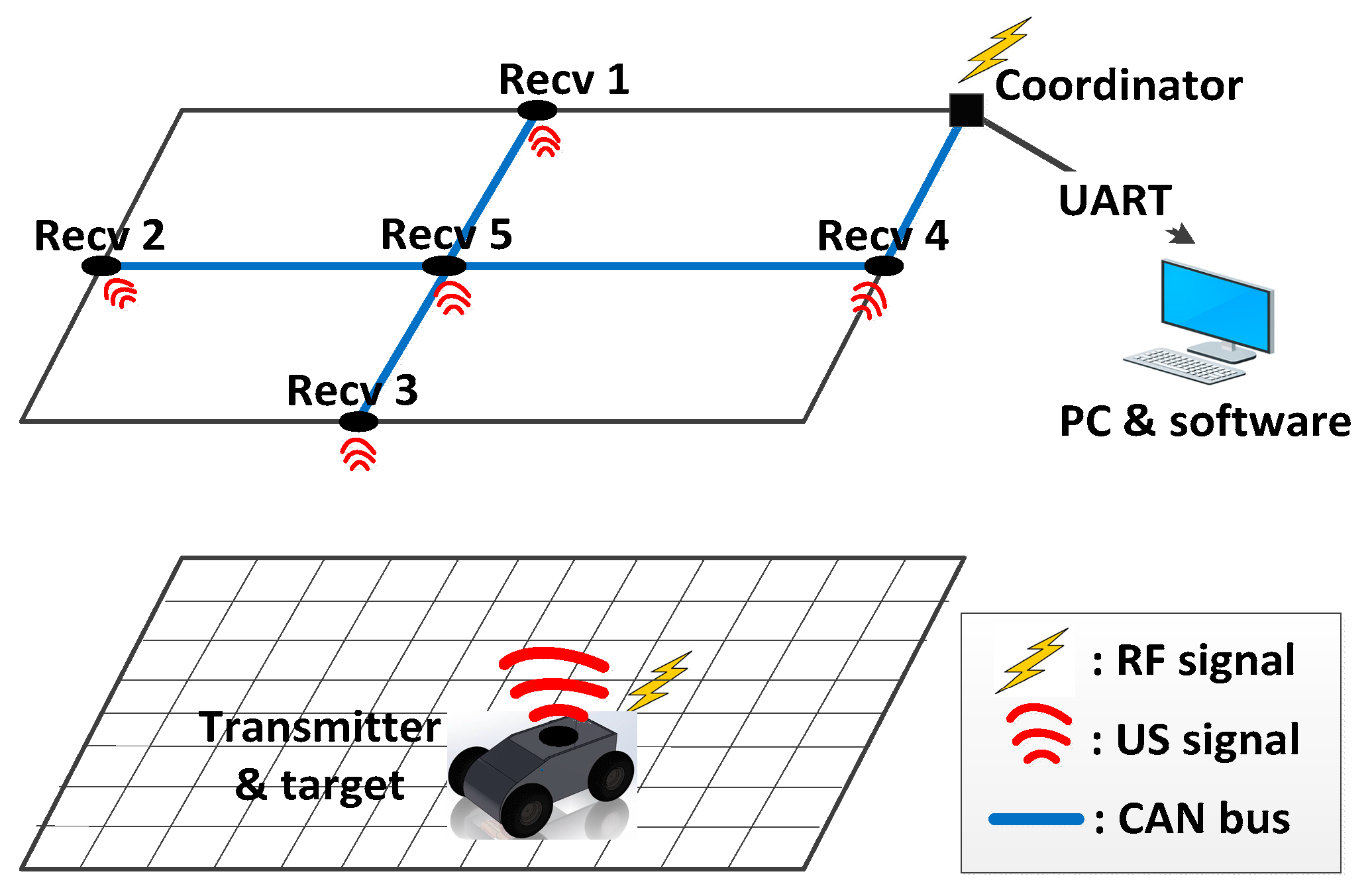
Figure 2.
Collision solving on the Controller Area Network (CAN bus) of 3 devices.

Figure 3.
Standard CAN bus.

Figure 4.
Extendable receiver network design of the SNSH system with a CAN network.

Figure 5.
(a) Schematic of ultrasonic (US) driver; and (b) US transmitter signal.

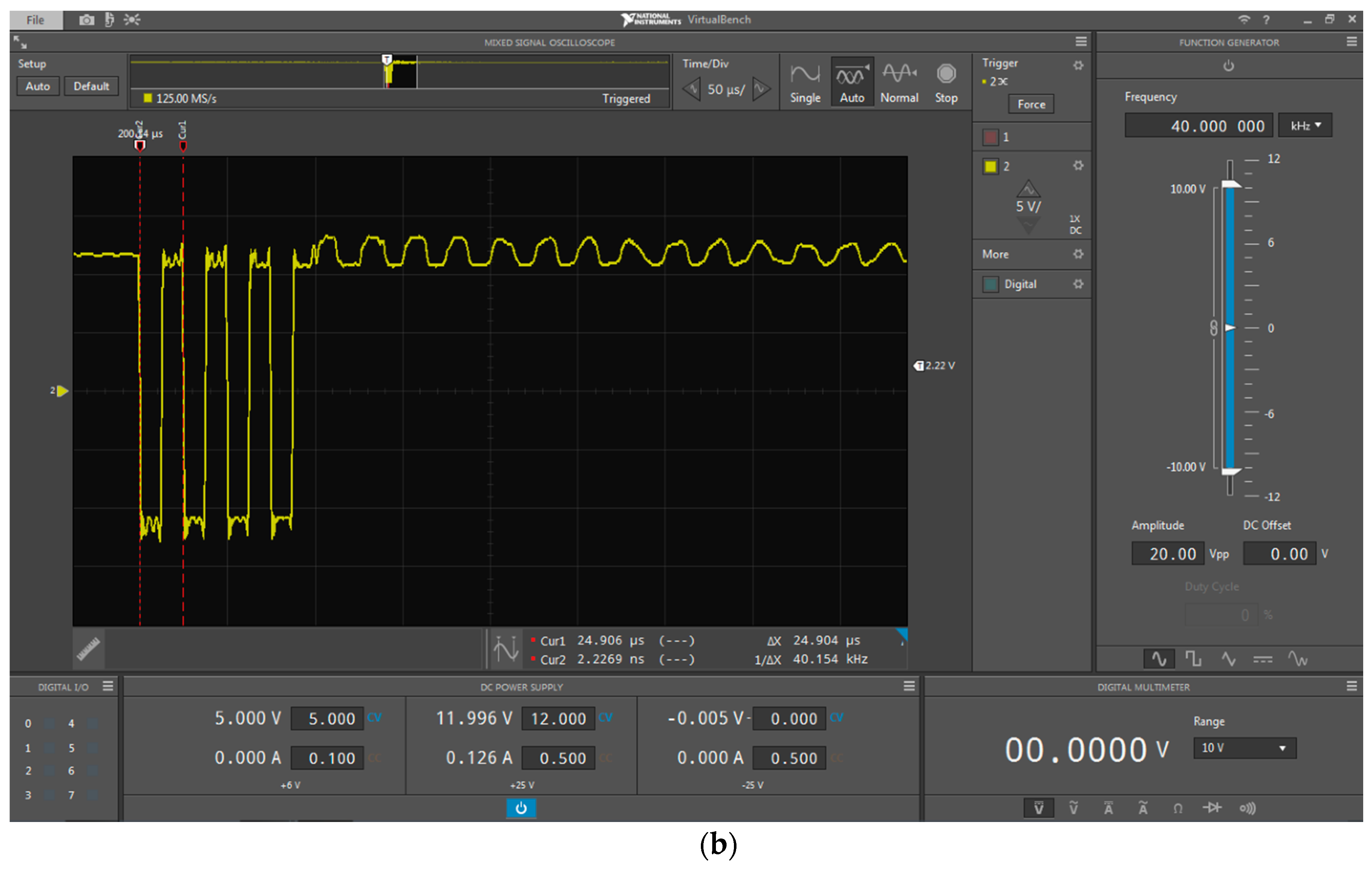
Figure 6.
(a) Amplifier and Filter circuit; as well as the (b) US receiver signal after pre-processing.
Figure 6.
(a) Amplifier and Filter circuit; as well as the (b) US receiver signal after pre-processing.

Figure 7.
MATLAB model of the sine wave detector in the time domain.

Figure 8.
MATLAB simulation results with a real wave signal at a sampling rate of 1.4 Mega-Samples Per Second (MSPS).
Figure 8.
MATLAB simulation results with a real wave signal at a sampling rate of 1.4 Mega-Samples Per Second (MSPS).

Figure 9.
MATLAB simulation showing the comparison of the Linear Least Square (LLS) and Nonlinear Least Square (NLS) algorithms.
Figure 9.
MATLAB simulation showing the comparison of the Linear Least Square (LLS) and Nonlinear Least Square (NLS) algorithms.

Figure 10.
Block diagram of the processing sequence in the receiver node.
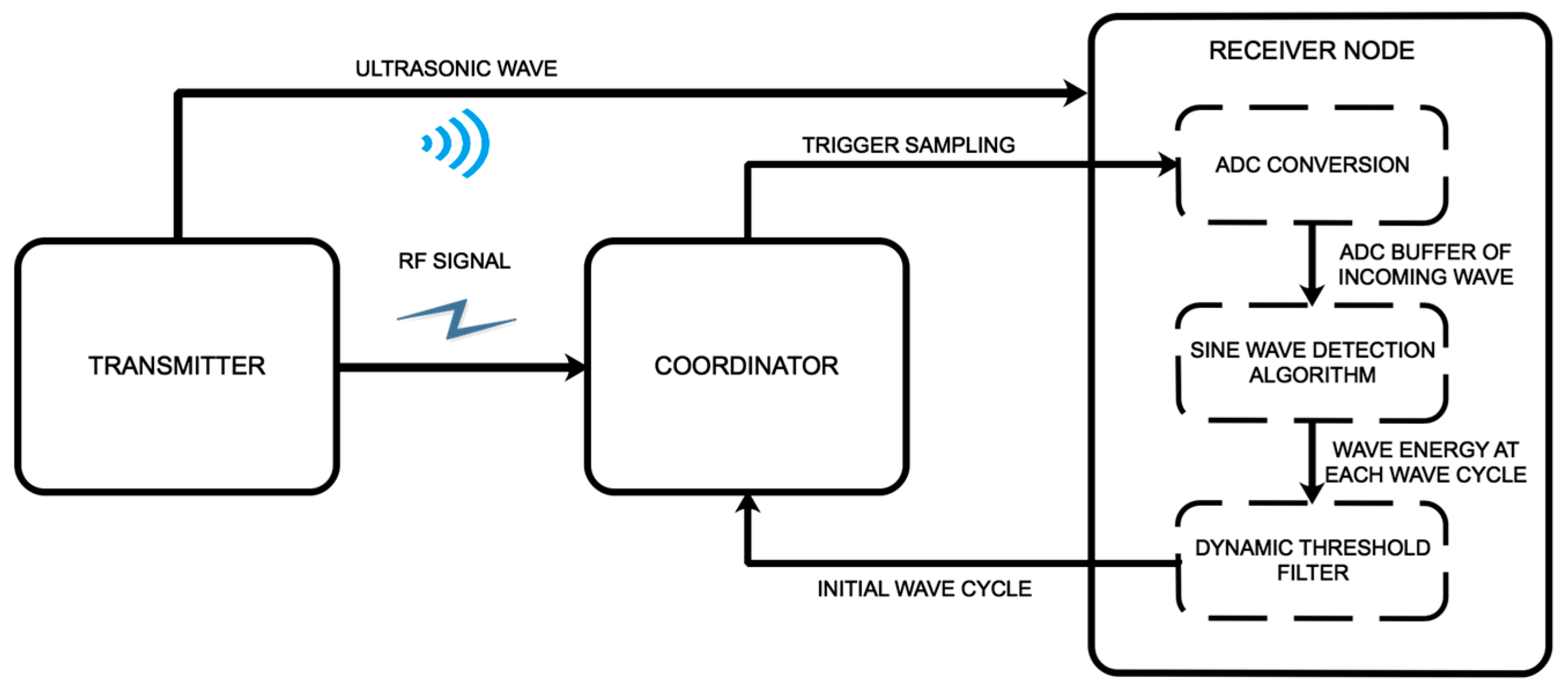
Figure 11.
Two steps in the Dynamic Threshold Filter.

Figure 12.
Experimental setup of the: (a) transmitter, (b) receiver and (c) distance measurement.

Figure 13.
Operation flow of the current demo system.
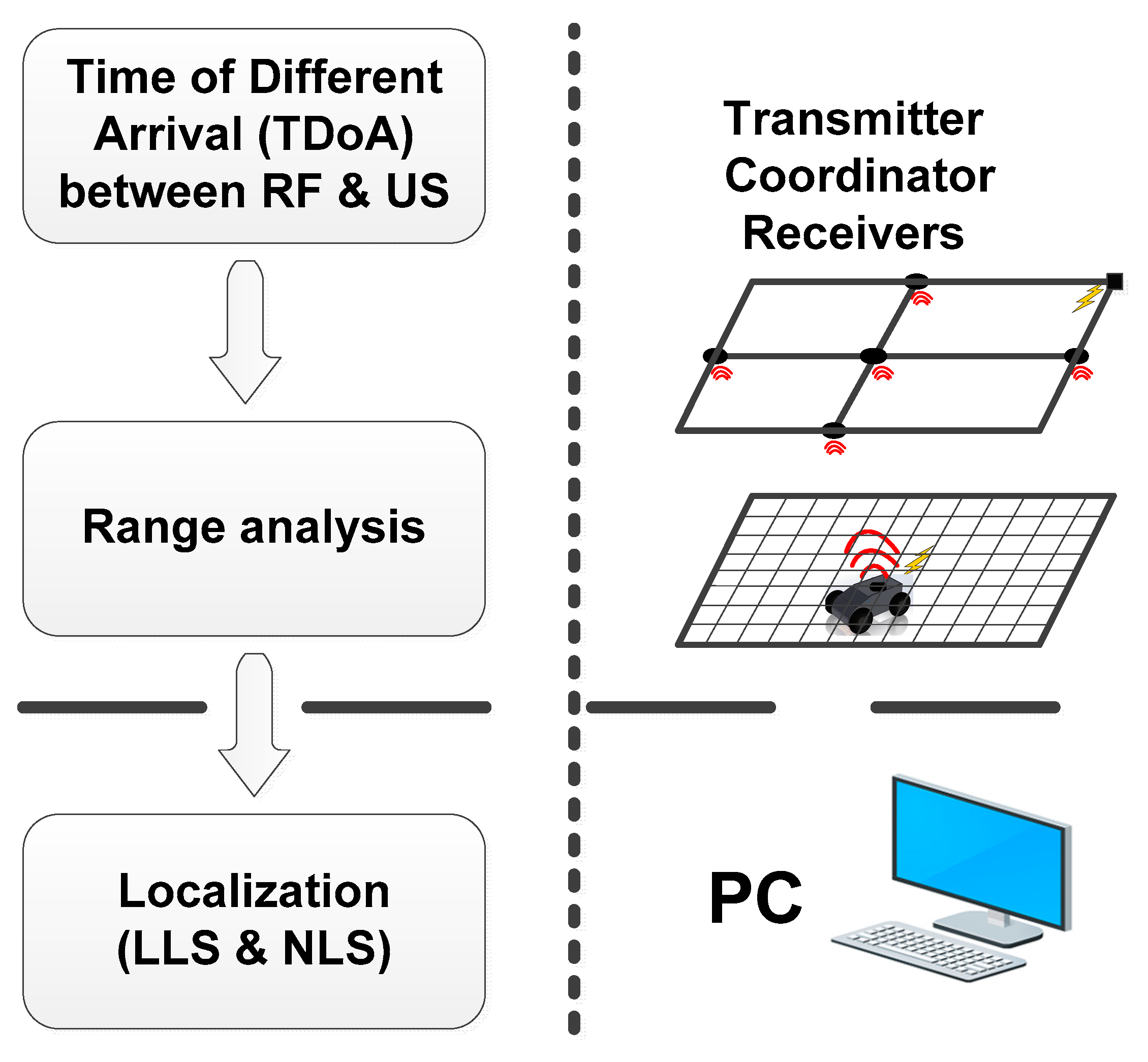
Figure 14.
Cumulative distribution function (CDF) of the Euclid distance error.

Figure 15.
Experimental set-up for moving targets.
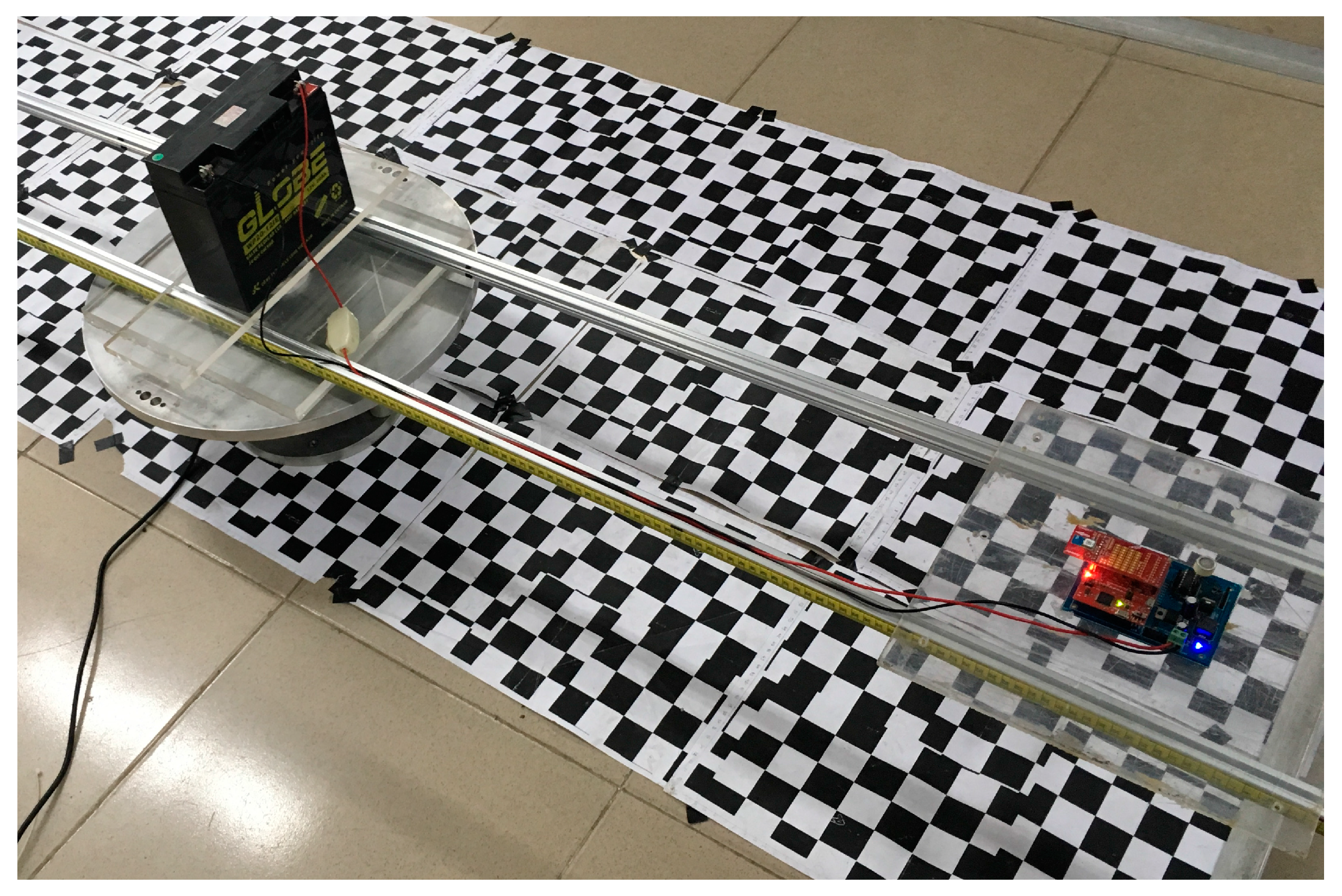
Figure 16.
Moving target positioning result (Center I(100, 100) and Radius R = 93 cm).

Figure 17.
Positioning error result along the X-axis, Y-axis and Euclidean distance.

Table 1.
Experimental results for distance measurement and comparison (range of up to 6 m).
| Methods | Average Error (mm) | Maximum Error (mm) |
|---|---|---|
| Proposed method (Sine wave detector) | 2.18 | 6.7 |
| Frequency Shift Keying and Correlation (Single Transmitter at 12 V, Multiple Access Receiver [22] | 8 | 20 |
| Correlation (Portable Ultrasonic Indoor) [34] | 0.9 | ≈2 |
| Sampling instant, detect maximum amplitude (sample rate = 32 kHz) [23] | 4.5 | 8.921 |
| Parabolic interpolation (sample rate = 32 kHz) [23] | 2.11 | 4.172 |
| Parabolic interpolation and phase correction (sample rate = 32 kHz) [23] | 1.692 | 7.528 |
| DSSS (Single-Access Ranging) [24] | Not mentioned | 10 |
| FHSS (Single-Access Ranging) [24] | Not mentioned | 15 |
Table 2.
Coordinate of reference nodes (in centimeters).
| Reference Node | R1 | R2 | R3 | R4 | R5 |
|---|---|---|---|---|---|
| Coordinate | (105, 5.8, 206.4) | (204.3, 105.5, 206.4) | (105.5, 204.5, 206.4) | (5.9, 105, 206.4) | (105, 105, 190) |
Table 3.
Evaluation of LLS and NLS in our experiments and comparison to other systems.
| Method | Average Error (mm) | Max Error (mm) |
|---|---|---|
| LLS (proposed system) | 13.3 | 33.6 |
| NLS (proposed system) | 12.0 | 29.7 |
| Cricket version 2 [10,11] | 10–30 | Not mentioned |
| Active Bat [8,9] | 80 | ~140 |
| Dolphin [35] | 150 | Not mentioned |
| iLoc [36] | 20 | 100 |
| SNoW Bat [37] | 15.0 | Not mentioned |
| Portable Ultrasonic Indoor [34] | 3.4 | 3.9 |
| Indoor localization application of Frequency Shift Keying and Correlation method [23] | Not mentioned | 50 |
© 2017 by the authors. Licensee MDPI, Basel, Switzerland. This article is an open access article distributed under the terms and conditions of the Creative Commons Attribution (CC BY) license (http://creativecommons.org/licenses/by/4.0/).
Share and Cite
MDPI and ACS Style
Nguyen, T.-S.; Nguyen, T.-N.; Tran, Q.-S.; Huynh, T.-H. Improvement of Ultrasound-Based Localization System Using Sine Wave Detector and CAN Network. J. Sens. Actuator Netw. 2017, 6, 12. https://doi.org/10.3390/jsan6030012
AMA Style
Nguyen T-S, Nguyen T-N, Tran Q-S, Huynh T-H. Improvement of Ultrasound-Based Localization System Using Sine Wave Detector and CAN Network. Journal of Sensor and Actuator Networks. 2017; 6(3):12. https://doi.org/10.3390/jsan6030012
Chicago/Turabian StyleNguyen, Tan-Sy, Trong-Nghia Nguyen, Quoc-Sang Tran, and Thai-Hoang Huynh. 2017. "Improvement of Ultrasound-Based Localization System Using Sine Wave Detector and CAN Network" Journal of Sensor and Actuator Networks 6, no. 3: 12. https://doi.org/10.3390/jsan6030012
Note that from the first issue of 2016, this journal uses article numbers instead of page numbers. See further details here.