The Sensor Network Calculus as Key to the Design of Wireless Sensor Networks with Predictable Performance

1
Distributed Computer Systems (DISCO) Lab, University of Kaiserslautern, 67663 Kaiserslautern, Germany
2
Huawei European Research Centre (ERC), 80992 Munich , Germany
*
Author to whom correspondence should be addressed.
J. Sens. Actuator Netw. 2017, 6(3), 21; https://doi.org/10.3390/jsan6030021
Submission received: 8 August 2017
/
Revised: 1 September 2017
/
Accepted: 5 September 2017
/
Published: 12 September 2017
(This article belongs to the Special Issue QoS in Wireless Sensor/Actuator Networks and Systems)
Abstract
:In this article, we survey the sensor network calculus (SensorNC), a framework continuously developed since 2005 to support the predictable design, control and management of large-scale wireless sensor networks with timing constraints. It is rooted in the deterministic network calculus, which it instantiates for WSNs, as well as it generalizes it in some crucial aspects, as for instance in-network processing. Besides presenting these core concepts of the SensorNC, we also discuss the advanced concept of self-modeling of WSNs and efficient tool support for the SensorNC. Furthermore, several applications of the SensorNC methodology, like sink and node placement, as well as TDMA design, are displayed.
1. Introduction
Many applications of wireless sensor networks (WSN) require timely actuation. For example, industrial process automation typically consists of a multitude of sensors and actuators that are required to interact in a very clearly-defined manner with respect to their timing. Traditionally, in this environment, real-time conditions have to be met. While using wireless communications and the increased complexity of modern factories makes hard real-time a more elusive goal, there is still a need for a predictable timing behavior of the system in order to avoid catastrophic behavior. Furthermore, WSNs have been proposed in the context of emergency response systems. Again, it is obvious that predictable timing behavior is key to the acceptance of such systems. More generally, many envisioned applications of cyber-physical systems (CPS) typically can be viewed as closed-loop systems [1], in terms of control theory, such that the sensing often becomes time-critical in order to ensure the stability of the system. As in many of the visions of CPS, using WSNs is an integral part for the sensing requirements, it can hardly be overemphasized that predictable timing is a necessity for WSNs in that context, as well. Consequently, a mathematical methodology to dimension, operate and control the timing behavior in WSNs is of outmost importance.
There is a clear trend for WSNs to become of ever larger scale, and some examples can be found in the CitySee project [2], the GreenOrbs project [3] and more generally in the emergence of the Internet of Things (IoT), which partially can be seen as a world-wide sensor network (with many sensors using wireless communication). Hence, a second key criterion for WSNs is the scalability of its basic functions and, in particular, of the mathematical framework to analyze its timing behavior. To that end, there is a clear need for a fast mathematical methodology to predict the timing behavior in WSNs.
In 2005, the sensor network calculus (SensorNC) was proposed as such a mathematical methodology [4], and in more than a decade, it was developed to meet the special requirements of time-sensitive, large-scale WSNs. Mathematically, it can be viewed as a special instance of the general network calculus, which itself is based on a min-plus algebraic formulation for the performance analysis of queueing networks as typical in packet-switched networks [5,6].
The goal is to have a mathematical framework that allows one to compute useful performance characteristics of WSNs such as message transfer delays, required buffer sizes and link capacities, but also duty cycle durations, to name some of the most prominent ones. Sometimes, we may require absolute values for, e.g., delays, if a certain application has hard real-time requirements, but sometimes, it may also suffice to have a representative relative metric in order to compare different design alternatives of a WSN before its deployment, for instance.
To that end, the SensorNC was customized in several dimensions and also extended over the general network calculus to capture the special requirements of WSNs, e.g., in-network processing. The goal of this article is to provide an overview of the efforts in over a decade of the development of the SensorNC framework, emphasizing the most important milestones in this.
In the following section, some background on the general network calculus framework is provided, in order to alleviate the introduction of the basic SensorNC methodology in Section 3. Advanced concepts of the SensorNC, in particular, in-network processing, are presented and illustrated in Section 4. Section 5 provides an overview of the self-modeling capabilities of WSNs that employ SensorNC. In Section 6, the important aspect of tool support for the SensorNC is discussed. Clearly, a mathematical framework such as the sensor is only as useful as the problems it can solve, and thus, we present several examples of SensorNC applications in Section 7. Section 8 provides a discussion and some concluding remarks.
2. Background on Network Calculus
We start with the necessary background on network calculus, before we introduce its customization in the WSN context in the following section.
2.1. Modeling of Flows and Performance Characteristics
Network calculus models the sequence of packets that define a flow’s data arrivals as non-negative, wide-sense increasing functions. These cumulatively count arriving data over time:
A flow’s input, as well as its output from a system are of interest to performance modeling. We denote the input up to time t as and the output as . If both count the data of the same flow, we demand , i.e., the flow’s output from system is caused by the input to . This causality preservation is known as the flow constraint of network calculus.
The flow definition and its causal transformation from system input to output enables us to define first the performance characteristics.
Definition 1.
(Backlog and delay) Assume a flow with input function R traverses a system and results in the output function . The backlog of the flow at time t is defined as:
The (virtual) delay for a data unit arriving at at time t is defined as:
2.2. Network Calculus Performance Analysis
Network calculus operates on bounding functions for flow arrivals. These are derived from the above input functions; yet, they are not defined over the time t that passed until the observation of the flow. Instead, they are defined over the duration of an observation d. These bounding functions are called arrival curves.
Definition 2.
(Arrival curve) Given a flow with input function R, a function is an arrival curve for R iff:
SensorNC often restricts the set of arrival curves to token-bucket-shaped traffic:
Curves of can easily be applied to bound the typical behavior of wireless sensor nodes. Assume a node periodically measuring its environment to report data. The maximum size of a measurement translates to parameter b that bounds the flow’s burstiness. The bound on the subsequent data reporting rate is where p denotes the sensing period.
Analyzing a network requires transformations of the bounding functions of (sensor) network calculus. Operations in -algebra have been established; see [5,6,7], respectively. The most important operations of this -algebraic framework over are presented in the following.
Definition 3.
-operations) The -algebraic aggregation, convolution and deconvolution of two functions are defined as:
Note that deconvolution is not exactly dual to convolution [6].
Aggregation of flows that cross a common system requires aggregating their arrival curves. In SensorNC, the flow aggregate’s arrival curve can be computed easily if each individual flow is constrained by a token-bucket arrival curve.
Corollary 1.
(Arrival curve aggregation in SensorNC) For the aggregation of n arrival curves of , it holds that:
In addition to flows, network calculus also operates on functions bounding the service capabilities of a system . These so-called service curves are defined over the duration of observation, as well. They bound the worst-case transformation of an input function to an output function.
Definition 4.
(Service curve) If the service provided by a system for a given input function R results in an output function , we say that offers a service curve β iff:
In SensorNC, service is often characterized by rate-latency functions from:
Rate-latency functions can model TDMA channel access [8] and duty cycling [9] in wireless sensor networks.
When data are queued to be forwarded and service capacity is available, many systems guarantee a greater amount of service than the one of Definition 4. Thus, they fulfil a stricter definition of service curves. These service curves allow for some computations that those from the general service curve model of Definition 4 do not.
Definition 5.
(Strict service curve) Let . System offers a strict service curve β to a flow if, during any backlogged period of duration d, the output of the flow is at least equal to .
Network calculus often computes results for one specific flow. In cases where this flow competes for a system’s resources with other flows, a bound on its resource share needs to be derived. This left-over service curve can only be computed from a strict service curve.
Theorem 1.
(Left-over service curve) Consider a system that offers a strict service curve β. Let be crossed by two flows with arrival curves and , respectively. Then, ’s worst-case residual service share under arbitrary multiplexing at system , i.e., the left-over service curve for the flow of interest, is:
As stated above, service curves bound the transformation of an input function to an output function . Given an arrival curve for , they can also be applied to compute an arrival curve for , a so-called output arrival curve:
Theorem 2.
(Output arrival curve) Assume a flow f has an arrival curve α, and consider f traversing the system offering a service curve β. After being transformed by , i.e., at the system’s output, f is bounded by the arrival curve:
Note that deconvolution is not closed in as . Therefore, we slightly augmented the operation such that its result is guaranteed to pass through the origin. Other performance bound computations are not affected by this adaptation.
Theorem 3.
(Performance bounds) Consider a system that offers a service curve β. Assume a flow f with arrival curve α traverses the system. Then, we obtain the following performance bounds for f:
Last, we present a central result of network calculus: the concatenation theorem. Concatenation allows one to logically transform a tandem of systems into a single system whose capabilities are bounded by a single service curve.
Theorem 4.
(Concatenation theorem for tandem systems) Consider a flow that traverses a tandem of systems , . Each offers a service curve to the flow. Then, the concatenation of the n systems offers a service curve to the flow.
A system-by-system analysis of delay and backlog bounds that applies Theorems 2 and 3 does not guarantee tight results. In contrast, the concatenation theorem facilitates tightness of bounds by deriving the tandem’s end-to-end service curve for the flow crossing it. In particular, bounds scale linearly in the number of crossed systems. This phenomenon is known as pay bursts only once [6].
An overview of the network calculus notation is provided in Table 1.
3. The Sensor Network Calculus
Provision of worst-case bounds on performance measures, such as the maximum delay that any flow in a WSN experiences, can be achieved by the sensor network calculus (SensorNC) framework. It was first presented in [4]. This work constitutes the first step towards concise worst-case analysis of WSNs. The initial SensorNC was based on the analysis of single servers in isolation; end-to-end performance bounds were derived by the addition of the crossed servers’ bounds. The concatenation theorem from conventional network calculus and thus a holistic view on the WSN was not applied (yet). This is due to the fact that the typical sink tree structure of the network does establishes an interference pattern of flows that does not allow for a direct application of the concatenation theorem. Additively-derived results are known to be more pessimistic and so are the performance bounds. Later work on SensorNC was then targeted to taking advantage of the concatenation result.
3.1. Sensor Network System Model
WSNs are often oriented towards a single base station such that the employed routing protocol can form a sink tree. This commonly-found class of operations can be abstractly modeled as shown in Figure 1. Only traffic from sensors to the base station is explicitly taken into account in this model. The majority of traffic flows in this direction. Traffic in the opposite direction, e.g., topology control messages or node configurations, can be considered in the service curves for sensor-to-sink communication; for instance, by assuming strict priority. Overall, the network calculus model arranges the sensor nodes as servers in a directed acyclic graph as depicted in Figure 1.
The system model takes the following aspects into account: each sensor senses its environment, reports data to the sink and forward measurements generated by other sensors in the network, i.e., the traffic seen by any sensor i consists of an input function derived from its own sensing and, in case it is not a leaf node in the sink tree, the forwarded data from its child nodes , ..., , where denotes the number of these nodes connected to sensor node i. As all of this input data are forwarded by sensor i, an output function results. This output function is processed by sensor i’s parent node.
3.2. Incorporation of Network Calculus Components
In this section, we incorporate the basic network calculus components, i.e., arrival curves and service curves, into the network system model. We make use of the simplicity of the SensorNC sink tree where each sensor has exactly one parent node. For a detailed treatment of modeling generic feed-forward networks, see [10].
Each sensor in the network is crossed by at least one flow. Their aggregate defines the total input to sensor i, . The total input function is composed by the sensor’s sensed input and the output of its child nodes:
We can derive an analogous description with network calculus arrival curves and operations applied to them:
where denotes the arrival curve for . It is composed of the arrival curve for the input sensed by sensor i, , and the aggregation of its child nodes’ output arrival curves. As an example, we could use simple token-bucket functions to model these inputs.
Next, service curves need to be incorporated. Specifying them is subject to the packet scheduling applied by the respective server. In a WSN, an additional impact factor is the link layer characteristics. For instance, duty cycling may be applied to achieve predefined energy-efficiency targets and thus impacts the service curve by periodical unavailability of the medium access. We model such a periodic service curve in the following. Assume the full medium capacity C is periodically available after an initial delay T, i.e., a TDMA medium access pattern results after this delay (see Figure 2). Let the TDMA frame duration be f and assume a sensor node receives s time units of service within a frame. From this information, we can compute T, the maximum initial medium access latency that can be experienced, as . To establish independence from the start of observation, the sensor node cannot be assumed to receive service during an initial duration of observation of T, and the service curve is zero. Then, the node receives service for the duration of its share of the TDMA frame. That is, from T to , the service curve will have a linear segment of slope C until it reaches . For the remainder of the TDMA frame, i.e., from to , service is unavailable again, and the service curve remains at . With the start of the next TDMA frame, the shape of the service curve from T to is repeated; it actually repeats indefinitely with a period of f. A similar service curve structure was proposed for 802.15.4 networks [11]. This curve can be approximated with a rate-latency service curve consisting of only two linear segments [12,13]: with and . In Figure 2, this fluid version of the TDMA service curve is labeled .
3.3. Calculation of Network-Internal Traffic Flow
When incorporating the required network calculus components into the system model, we added output arrival curves of servers. Next, we present their computation in a sink tree network. The traffic a sensor node i forwards to its parent sensor node is constrained by arrival curve:
Equation (3) can be expanded to a recursive computation by considering the output of child nodes as given in Equation (2). However, making use of the sink tree structure of the network allows for the iterative computation of all given by Algorithm 1. Note that this procedure requires perfect knowledge about the sink tree structure to correctly handle aggregation of flows in Step 3.
| Algorithm 1: Computation of network-internal traffic. |
|
3.4. Calculation of Performance Bounds
After the arrival curves for network-internal traffic flows are computed, we can also compute performance bounds according to Theorem 3. For instance, the buffer requirements of sensor nodes , a performance metric of interest for the bottleneck nodes directly below the sink:
Similarly, the per-node delay bounds are computed with the given arrival and service curves:
These derivations constitute SensorNC’s original node-by-node computation of performance bounds [4]. In order to compute a flow’s end-to-end delay bound, the per-node delay bounds along its path are added up. This approach is known as the total flow analysis (TFA) of network calculus. It does not benefit from the pay bursts only once (PBOO) phenomenon.
A more sophisticated approach is required to benefit from more advanced network calculus phenomena and thus derive more accurate end-to-end delay bounds. PBOO can be achieved by first computing the left-over service curve for every server on the flow of interest’s path (application of Theorem 1). Then, these left-over service curves are concatenated with Theorem 4 before the delay bound is computed. This approach is known as the separated flow analysis (SFA) of network calculus and its application in SensorNC was proposed in [11] where the improvement over TFA is also given.
The third phenomenon to tighten end-to-end delay bounds in network calculus is called pay multiplexing only once (PMOO). In case cross-traffic flows are multiplexed with the flow of interest on multiple consecutive nodes (as is common in sink trees), it prevents their burstiness from impacting the derivation multiple times. This is achieved by applying the concatenation theorem as early as possible, i.e., before the application of Theorem 1.
We illustrate the impact of advances in the SensorNC analysis by an example. Consider the simple sink tree network depicted in Figure 3. Computing delay bounds proceeds as discussed above: TFA computes an additive end-to-end delay bound; SFA computes per-node left-over service curves; and PMOO concatenates before the left-over computation:
Assume rate-latency service curves and token-bucket arrival curves . Then, we compute the following delay bounds: , , . As expected, PMOO results in the most accurate bound. In our example, TFA outperforms SFA, yet only because it implicitly assumes FIFO multiplexing (when computing the horizontal deviation for the total flow aggregate at each node) instead of the more pessimistic arbitrary multiplexing assumption of SFA and PMOO. Nevertheless, in larger sink tree networks, application of the SensorNC SFA usually outperforms the TFA [11].
More details about the PMOO analysis for general feed-forward networks, including its relation to other network calculus analyses, as well as an in-depth discussion, can be found in [14,15]. In sink tree networks, a specialized version can make use of the network structure. Similar to Algorithm 1, perfect knowledge about the locations of aggregation of flows and the lack of demultiplexing due to their common sink are exploited in Algorithm 2.
| Algorithm 2: Sink tree PMOO analysis. |
|
4. Advanced SensorNC: In-Network Processing
In the previous section, sensor nodes were abstracted as simple communication resources. Clearly, this can only be a very coarse-grained abstraction. In many wireless sensor networks, some form of in-network processing is applied to the data before it is delivered towards the sink. This is, e.g., often done in order to save energy by data aggregation. Therefore, computational resources, i.e., the usage of the processing unit, should be factored into the SensorNC model of nodes. As the workload units differ between communication and computation, we need new modeling elements that translate between the usage of communication and computational resources. In [16,17], such elements have been introduced as workload transformations or scaling elements, respectively. Though being conceptually very simple components that translate, for instance, a number of bytes received from other sensors into a worst-case sequence of processing steps, they complicate the end-to-end analysis since they build up “walls” between the different resources, effectively inhibiting the direct usage of the concatenation result. Nevertheless, we show that an end-to-end-analysis can still be performed by moving the scaling elements such that simultaneously, the analysis becomes feasible and no compromise of the worst-case occurs.
4.1. Background on Data Scaling in Network Calculus
Next, we introduce the necessary background on scaling elements as presented in [17].
Definition 6.
(Scaling function) A scaling function assigns an amount of scaled data to an amount of data a.
Scaling functions are a very general concept and serve as a model for any kind of data transformation in a network calculus model. Note that they do capture any queueing-related effects; consequently, scaling is assumed to be done infinitely quickly. Queueing effects are captured by the service curve element.
Definition 7.
(Scaling curves) Given a scaling function S, two functions are minimum and maximum scaling curves of S iff ; it applies that:
In [17], it is shown that maximum scaling curves should be sub-additive and minimum scaling curves super-additive. Otherwise, they can be enhanced by computing their super-additive resp. sub-additive closure.
Theorem 5.
(Alternative systems) Consider the two systems in Figure 4, and let be the input function. System (a) consists of a server with minimum service curve β whose output is scaled with scaling function S, and System (b) consists of a scaling function whose output is input to a server with minimum service curve . Given System (a), the lower bound of the output function of System (b), , that is , is also a valid lower bound for the output function of System (a) if:
The implication of this theorem is that performance bounds for System (b) are also valid bounds for System (a), that is a scaling element can be moved in front of a service curve element if we apply the minimum scaling curve to the service curve of the respective component.
The effect of scaling on the arrival constraints of a flow is stated in the following corollary.
Corollary 2.
(Arrival constraints under scaling) Let R be an input function with arrival curve α that is fed into a scaling function with maximum scaling curve . An arrival curve for the scaled output from the scaling element is given by:
Not that, if the arrival curve and maximum scaling curve are tight, then the scaled arrival curve also is.
4.2. Data Scaling in Sink Trees
With the aid of the scaling element, a much more comprehensive model of a WSN that integrates the processing besides the communication resources can be facilitated. Figure 5 illustrates the advanced SensorNC model.
Besides the scaling elements, a multiplexing element is also introduced. The multiplexing element enables an explicit modeling of the aggregation of a set of flows, for instance arbitrary, FIFO or using strict priorities between flows. Thus, data flows arriving from predecessors in the sink tree are multiplexed and then scaled in order to transform them into local processing demand. The local sensing data are taken into account by a scaling element just before they are multiplexed with the other data flows. The overall aggregate is then processed by the sensor node modeled by a service curve . As the amount of data that are forwarded downstream depends on how the processing is, for example, able to compress the data flow by, e.g., data aggregation, another scaling element translates the flow back to the required communication resources before it is served by the communication subsystem of the sensor node represented by another service curve element .
The challenge of this new advanced SensorNC model lies in the scaling elements that prevent an immediate end-to-end analysis following the PMOO principle. Yet, building on the theory from the previous subsection, we can shift all of the scaling elements upstream across service curve elements in order enable a true (PMOO) analysis again. The only remaining challenge is the shifting of scaling elements across multiplexers. In the following theorem, we prove a sufficient condition that allows this shifting without compromising the worst-case semantics.
Theorem 6.
(Shift of the scaling element across the multiplexer) Assume a situation as depicted in Figure 6, i.e., two flows are multiplexed and then fed into a scaling function S with maximum scaling curve and minimum scaling curve . Provided that the minimum scaling curve is super-additive and the maximum scaling curve is sub-additive, we can transform System (a) into System (b) without improving the worst-case scenario in System (b) over the one in System (a).
Proof.
This can be found in [18]. ☐
Consequently, all of the scaling elements can be moved to the sources of traffic. In principle, all of the input to the system is translated to the same resource units before entering a system of “homogenized” servers, such that we can apply the end-to-end concatenation-based techniques from Section 3.
4.3. Effect of Scaling Element Movement on Model Components
To make the method of scaling element movements more tangible, let us briefly illustrate its effect on the other modeling components. We base this discussion on simple, yet very commonly-used modeling component instances. In particular, we assume token-bucket arrival curves as arrival curves and rate-latency service curves . As the maximum scaling curve, we also assume a token-bucket function , and as minimum scaling curve, we take a rate-latency curve . This form of maximum scaling curve is sensible as it can capture the fact that a small number of bytes received might result in a high demand on the computational resources, whereas for larger amounts of received data, this effect degrades. For the minimum scaling curve, the reasoning is just the other way around. Now, when we shift the scaling element across a service curve element, we need to compute the new service curve as:
where ∘ denotes the concatenation of functions. Hence, the resulting service curve is again of the rate-latency type with a suitably scaled rate and an increased latency.
If the scaling elements have been shifted to the sources of traffic, i.e., the sensing inputs, their effect on the arrival constraints can be calculated as:
Thus, the arrival curves of the scaled traffic flows remain token buckets with again suitably-scaled rate and increased bucket depths.
Moving scaling elements across multiplexers has been discussed in the previous section and does not alter the multiplexers. That is true for any multiplexing, be it arbitrary, FIFO, priority-based or any other.
4.4. Numerical Experiment
In this section, we perform a set of numerical experiments to investigate the performance benefits of a holistic SensorNC analysis using the PMOO result and the shifting of scaling elements from Section 4.2 compared to a node-by-node approach based on the total flow analysis (TFA) from Section 3.4.
4.4.1. Experimental Design
At first, we create a set of WSN topologies by randomly placing n sensor nodes on a square field using a uniform random distribution. All nodes have a transmission range of 20 m such that connectivity is likely achieved (if not, the corresponding topologies are discarded). The sink node is in the middle of the sensor field, and the sink tree is built from a shortest path algorithm. For statistical significance, we evaluate 10 topologies for each experiment scenario. In all experiments, we selected nodes and a sensor field of 100 m.
The parameters relating to the sensor nodes resemble MICAz motes from Crossbow Technology Inc. (Milpitas, CA, USA) [19]. A transmission rate of 250 kbps is used; as MAC, we assumed a TDMA-based scheme that uses a duty cycle of 1% and a TDMA frame length of 100 ms. Thus, the communication service curve is given as . As the packet length, 36 B TinyOS packets are assumed. With respect to computational resources, the MICAz has an Atmel ATmega 128 L microcontroller operating at 8 MHz. Assuming an average of four cycles per instruction, its raw capacity amounts to 2 MIPS. Under the realistic assumption that the processor also performs other tasks, for instance network control operations, and that a power management scheme with certain sleep periods in low power modes is applied, we select its capacity for data processing to be 10% of its full capacity with a worst-case latency of 1 ms. Hence, the service curve for computation is given by .
From the scaling elements, we employ token-bucket functions for the maximum scaling curves and rate-latency functions for the minimum scaling curves. The maximum scaling curve that translates between communication and computation resources is set as , that is a received packet results in 5000 instructions, and deviations from this are captured by the bucket depth b, which varies in the experiments. The minimum scaling curve is set to , with the latency parameter T also being varied in the experiments. Along the same lines, maximum and minimum scaling curves for the translation between sensing and computation resources are set as and ; here a higher computational demand for sensing is assumed because raw sensing values are given priority. Rescaling computation into communication resource demand is selected to be roughly inverse to the other scaling elements while also capturing some compression because of, e.g., data aggregation.
The data arrival from local sensor are modeled by a token bucket , that is we assume a packet to be created every 10 s with a burst due to an instantaneous packet arrival.
Clearly, many of these settings seem somewhat arbitrary and differ from scenario to scenario, yet they are from realistic settings and should thus be fairly representative.
With the aid of the DISCO Deterministic Network Calculator [20,21], we next present the results from the comparison between holistic and component-wise analysis (the DISCO Deterministic Network Calculator is publicly available under https://disco.cs.uni-kl.de/index.php/projects/disco-dnc.)
4.4.2. Benefit of End-To-End Analysis
At first, in a baseline comparison, minimum and maximum scaling curves are assumed to be identical and pass through the origin. In Figure 7, we can observe the SensorNC outcomes in terms of delay bounds for the holistic and component-wise methods for 10 different random topologies with 100 nodes each.
The holistic PMOO is superior to the TFA, which results in delay bounds up to 1.9-times higher than for PMOO.
Sometimes, we cannot assume identical minimum and maximum scaling curves as in the previous experiment because of non-determinisms in the actual processing. However, often, we can use upper and lower bounds on the amount of processing that is required, i.e., we can model this by differing minimum and maximum scaling curves. However, this bounding may adversely effect the performance of the PMOO analysis method. In order to provide more insights into this, we next change the minimum and maximum scaling curves to be no longer passing through the origin, but move the maximum scaling curve a bit upwards and shift the minimum scaling curves to the right. Therefore, they are drifting apart from each other, i.e., we set the bucket depth parameters of the maximum scaling curves, as well as the latency parameters of the minimum scaling curves incrementally higher until certain limits are reached. These limits are: for , the maximum bucket depth is 240; for , the maximum latency is 0.006; for , the maximum bucket depth is 300; for , the maximum latency is 0.006; for , the maximum bucket depth is 0.006; for , the maximum latency is 240.
In Figure 8, for both methods, we can observe the average delay bounds for 10 random topologies under different expansion factors, with the expansion factor as the percentage of how much the drifting limits have used.
Again, the PMOO performs superior to the TFA, and a certain amount of drifting between maximum and a minimum scaling curve are reached. After this point, the TFA becomes actually better than the PMOO as the uncertainty about the scaling becomes too large. Therefore, it can be wise to perform both SensorNC analyses.
5. Towards Self-Modeling Sensor Networks
In large-scale WSNs, any form of centralized control is often undesired if not impossible. Instead, a self-organized paradigm is followed; thus, it is consequent to also perform the modeling in a distributed, network-internal manner. The model is supposed to allow the WSN to act accordingly, e.g., by distributed decision on the admission of certain additional sensing tasks.
For such a self-modeling with SensorNC, the two basic pieces of modeling information are: the residual service a sensor can offer, i.e., the left-over service curve, and the arrival curve valid for a flow at a certain location in the network. The left-over service curve is the result of an analysis that requires the bound on interfering traffic. Deriving the arrival curves for interfering traffic, on the other hand, requires executing the deconvolution of flow arrivals with (left-over) service curves according to the exact shape of the sink tree. For this reason, general network calculus relies on the global view of the network and thus does not support self-modeling in WSNs. In this section, we present a way how, in a restricted, but practically very relevant setting, the SensorNC computations can be distributed over the WSN’s sink tree network such that self-modeling is realized. We achieve self-modeling by rephrasing the SensorNC analysis, in particular the output arrival curve presented in Section 3.2 and Section 3.3, as well as the PMOO analysis in Algorithm 2 where these curves are used. In order to do so, we need to restrict the curve shapes for modeling and analysis to the oftentimes used rate-latency service curves and token-bucket arrival curves . Then, the three network calculus bounds can be computed as follows:
Corollary 3.
(Performance bounds in SensorNC) Consider a sensor node that offers a service curve . Assume a flow f with arrival curve traversing this node. Then, we obtain the following SensorNC performance bounds:
Calculating the bound on network-internal traffic at any location uses aggregation and deconvolution. Given the above restriction of curve shapes, the following property holds for the combination of these operations.
Lemma 1.
(Distributivity of with respect to +) For any and , it holds that:
Proof.
Let , and . From Corollary 3, it follows that:
If , we have , and for , we get:
☐
Moreover, the composition rule of follows from [6] by an argumentation similar to Lemma 1. The above distributivity and the composition rule allow one to compute the network internal output arrival curve of Algorithm 2 with a new SensorNC concatenation theorem.
Theorem 7.
(SensorNC concatenation theorem) Consider a sensor node in a sink tree that is crossed by a set of flows with arrival curves . For the purpose of their aggregate output arrival curve calculation, the share of service offered to each flow from its source to within this aggregate is the concatenation of the service on its path. Then, the entire flow aggregate’s output is bounded by
where is the location (index) of sensor node s on f’s path, and in reverse, denotes the sensor at location (index) i on f’s path. Applying Corollary 3 and the composition rule, we can rephrase the equation to:
with
Proof.
Can be found in [22]. ☐
Using this result in the PMOO analysis of Algorithm 2 requires separating the flow of interest from its interfering traffic. To do so, Theorem 7 can be applied to a the subset of flows not including the flow of interest.
This reformulated computation’s decisive improvement for a self-modeling WSN is the change from a total output arrival curve for an flow aggregate to an aggregate of flow-local results. The computations only make use of individual flow’s arrival curves and the service curves of servers they cross. Information about the sink tree network’s exact shape, merging locations with other flows or left-over service curves, are not required. Figure 9 illustrates the flow-locality of the computation.
Applying the new method from Theorem 7 instead of the conventional one of Section 3.3 has several practical advantages for self-modeling WSNs:
Complete model with low communication overhead: Flow-locality enables one to overcome the need for an additional protocol such as Deluge [23], distributing the information required to derive network-internal arrival curves and left-over service curves. Each flow’s arrival at a server can be calculated hop-by-hop without compromising accuracy. A flow can carry information about its current arrival bound as payload, pushing the information to all sensors concerned. From all of the flows crossing them, sensor nodes can derive their local delay bound and backlog bound, as well as their left-over service curves. Thus, the network model is updated continuously, i.e., independent of a polling interval, with only a small payload overhead.
Local reaction to changes: The flow-locality also affects the recomputation effort in the case of parameter modifications. Using the conventional method, the locality of a modified parameter did not matter much due to the complex setting of flow aggregation locations; a change to a single parameter always invalidated a large amount of the derivation’s intermediate results and triggered expensive recomputations, usually of the entire subtree. Theorem 7 prevents such an invalidation from spreading to flows not directly affected by a change, e.g., flows not crossing a sensor that adapted its rate, and thus enables a quick reaction to changes.
6. Tool Support
The DISCO Deterministic Network Calculator (DiscoDNC) [20,21] offers tool support for network calculus in general, as well as specialized SensorNC optimizations. For both, the DiscoDNC builds upon an implementation of piecewise linear curves and the network calculus operations. A recent overview of its core architecture can be found in [24].
The DiscoDNC implements the three analysis methods on the path of the flow of interest discussed in Section 3.4, TFA, SFA and PMOO analysis, as well as some more [25,26]. Additionally, the DiscoDNC provides methods to bound interfering flows’ descriptions when they enter the flow of interest’s path. Alternatives either implement the pay bursts only once principle (Section 2) or the PMOO principle. They either aggregate the interfering flows or execute a per-flow computation during the computation [27], and all alternatives can be augmented with an additional output burstiness restriction [28]. Thus, the DiscoDNC comprehensively covers a wide range of alternative analyses proceeding from generic network calculus.
For SensorNC, only a subset of these alternatives is relevant. For example, neither TFA nor SFA can outperform PMOO on the flow of interest’s path. On the other hand, SensorNC offers specific solutions exploiting the oftentimes used token-bucket arrival curves and rate-latency service curves and the network’s sink tree topology. For both of these specialized settings, the DiscoDNC implements separate code paths, as well. In particular, efficient computations of convolution and deconvolution of token-bucket arrival curves and rate-latency service curves are provided alongside the SensorNC concatenation theorem presented in Section 5. These specialized code paths are also suitable to demonstrate the reduced computational demand of SensorNC compared to generic network calculus [22]. Figure 10 shows such a comparison:
In Figure 10a, every flow’s delay bound in a homogeneous sink tree with 100 sensor nodes is computed. Arrival curves are set to ; service curves are ; and the sink tree is randomly created with a maximum of five child nodes per sensor, as well as a maximum sink tree depth of 20. Whereas an alternative approach to achieve flow locality for self-modeling results in considerably worse delay bounds, the generic network calculus approach without flow locality and the SensorNC approach presented in the previous section yield the same delay bounds.
For a second set of results, we randomly created 40 sink trees of sizes up to 1000 sensor nodes. Each flow in each sink tree network was analyzed with generic network calculus (no flow locality) and SensorNC. The reduction of computation times achieved by SensorNC is shown in Figure 10b. Whereas the reduction is negligible in very small sink trees, it first rapidly increases and stays at a level of about five-times, although slowly decreasing with the WSN’s size. Thus, the available tool support provided by the DiscoDNC shows that SensorNC can achieve the same accuracy as generic network calculus, yet at a fraction of the computational cost; a crucial improvement for deployment in self-modeling WSNs.
7. SensorNC Applications
In this section, we display several application examples where the SensorNC framework was instrumental.
7.1. Optimal Sink Placement
In many WSN applications, it is desired to collect the information acquired by sensors for processing, archiving and other purposes. The station where that information is required is usually the sink. For large-scale WSNs, a single-sink model is not scalable since message transfer delays, as well as energy consumption of the sensor nodes become prohibitive, due to the fact that most of the nodes would be far away from the sink, and thus, many hops must be traversed before the sink is reached. As a result, response times become excessive, and the lifetime of the WSN becomes very short. Therefore, it is sensible to deploy multiple sinks so that messages reach their destination with less hops, and consequently, response times are decreased and energy saved.
If sinks are placed in good locations, this can reduce traffic flow and energy consumption for sensor nodes. In particular, we focus on strategies to minimize the maximum worst-case delay, which is important for any timely actuation based on the information collected by a WSN.
In mathematical terms, we can pose the problem as follows:
with:
Here, n denotes the number of sensor nodes, and is the vector of their locations in the sensor field ; these locations are assumed to be given. The values are the worst-case delays for each sensor node i. By minimizing the maximum worst-case delay in the field, it is ensured that response times are balanced as much as possible. k is the number of sinks, and the vector contains their locations; these locations are the actual decision variables of the optimization problem. This is somewhat hidden by the fact that the delays are only indirectly, affected by the choice of the sink locations, because as a first-order effect, the are a function of the topology in which the WSN organized itself in the data flow towards the sinks and the arrival and service curves of the sensor nodes, denoted as and in the formulas above. While the arrival and service curves are parameters for a given WSN scenario, the topology is, in turn, a function of the nodes’ locations, the routing algorithm and the sinks’ locations , where however only the sinks’ locations are variable, and the other two are again given parameters. Note, in particular, that we assume the routing algorithm to be given and not to be subject to the optimization. Although this could in principle be done, it would aggravate the problem further and is therefore left for further study.
Therefore, in principle, we face a continuous optimization problem where the objective function is to minimize the maximum worst-case delay in the field subject to constraints that ensure that each sensor node is connected to a sink (possibly via multi-hop communication, determined by the routing algorithm), as well as some geographic constraints. Due to the highly non-linear, jumpy behavior of the worst-case delay function f and thus of the objective function, which results from the formulas derived by sensor network calculus, the direct solution of that optimization problem is practically infeasible.
Therefore, a heuristic strategy for the sink placement problem that minimizes the maximum worst-case delay in WSNs based on the sensor network calculus framework was developed: genetic algorithm-based heuristic for sink placement (GASP). The crucial insight used by the GASP is that the continuous optimization can be reduced to a combinatorial optimization by identifying so-called regions of indifference, in which any location results in the same delay performance, and thus, a single location for such a region can be selected as a candidate. More details can be found in [29,30].
The performance of the GASP was analyzed in comparison to two other strategies. One is an optimal strategy, called OSP , based on an exhaustive search over the set of candidate locations (only feasible in small scenarios) which serves as an upper bound for the performance achievable by the GASP, and the other one is a Monte Carlo-based strategy, called MCP , that should serve as lower bound on the performance that can be expected from the GASP.
7.1.1. Small-Scale WSNs: Comparison between OSP and GASP
In this set of experiments, we analyze the worst-case delay for GASP and OSP for different, but relatively small network sizes of 30, 50 and 100 nodes. The number of candidate locations for the sinks were about 450, 950 and 2200 for the 30-, 50- and 100-node network, respectively. The number of sinks was restricted to two, since for the 100-node network, this already meant that the OSP strategy had to evaluate 2,418,900 different combinations of sink placements. Each evaluation consists of 100 per-flow delay analyses, resulting in a total run-time of the OSP of several days. For the GASP, on the other hand, we chose a population size of 40 individuals, and the number of generations was set to 200, resulting in only 8000 different sink placements that where evaluated in only a few minutes. The worst-case delay results for the best sink placements found by the GASP and OSP are shown in Figure 11.
As can be observed, the GASP performs very well in comparison to the OSP: for the 30- and 50-node network, it actually finds the global optimum; only for the 100-node case, the best sink placement found by the GASP lies slightly above the one found by the OSP (8.02 s vs. 7.70 s). That should be considered a success of the GASP since with a computational effort that is several orders of magnitude lower than for the OSP, it achieves almost the same quality of solutions. Whether this holds true for larger-scale scenarios is difficult to assess as the OSP is prohibitively computationally expensive. Therefore, in the next subsection, we compare the GASP against the MCP in larger-scale networks.
7.1.2. Large-Scale WSNs: Comparison between MCP and GASP
The question we address in this experiment is whether the GASP constitutes a more intelligent search strategy than a pure random search like the MCP. In fact, there would even be the possibility that the MCP could outperform the GASP. This would be the case if the GA operators were poorly designed and would mislead the GASP in areas of the search space that are fruitless. Therefore, in a certain sense, the following experiments also validate the design of the GASP heuristic.
We investigate a 500-node network with up to seven sinks for 10 different scenarios, i.e., 10 different node distributions. For each of the scenarios, this resulted in approximately 13,000 candidate sink locations, so that at maximum, the search space becomes as big as . On the other hand, for the GASP, we used a population size of 100 with 100 generations until termination, resulting in 10,000 sink placements being evaluated for their worst-case delay. We allow the same amount of evaluations to the MCP. In any case, it is clear that this amount of sink placement evaluations constitutes only a tiny fraction of the overall search space.
The results (averaged over the 10 scenarios) of these experiments are shown in Figure 12. This analysis shows that the GASP performs better than the MCP at the same amount of computational effort. For the GASP strategy, the worst-case delay improves from 12 s to 5.7 s to 4.1 s to 3.2 s to 2.7 s to 2.3 s to 2.0 s for the one- to seven-sink scenarios, respectively. For the MCP, the worst-case delay improves from 14.1 s to 6.6 s to 5.0 s to 4.2 s to 3.3 s to 3.2 s to 2.5 s for the one- to seven-sink scenarios, respectively. The delay difference between the two strategies is roughly between 0.5 s and 2 s. This shows that the GA operators do something sensible as the GA search improves on the pure random search of the MCP. Besides, these numbers also give a feeling what the delay vs. number of sinks tradeoff looks like. Moreover, the confidence interval of MCP varies from 0.1 s to 1.2 s, whereas GASP varies from 0.05 s to 0.8 s. Obviously, providing a second sink improves the delay performance very much, whereas further sinks have a lesser effect on the maximum worst-case delay observed.
7.2. Node Placement Strategies
Node placement is a fundamental issue to be solved in WSNs. A proper node placement scheme can reduce the complexity of problems in WSNs, for example routing, data fusion, communication, etc. Furthermore, it can extend the lifetime of WSNs by minimizing energy consumption. In this section, we investigate the worst-case delay using SensorNC in random and deterministic node placements for large-scale WSNs under the following performance metrics. A more comprehensive investigation can be found in [31]. We consider three competitors: a uniform random, a square grid and a pattern-based tri-hexagon tiling (THT) node placement. We assume homogeneous sensor nodes.
7.2.1. Node Placement Schemes
During the design phase of WSNs, the designer only knows the number of sensor nodes, n. A circular field with radius R is considered in our experiments. Next, we introduce three node placement schemes.
Uniform Random
We choose a uniform random placement as one of the competitors. In the uniform random placement, each of the n sensors has equal probability of being placed at any point inside a given field, as shown in Figure 13a. For example, such a placement can result from throwing sensor nodes from an airplane, helicopter or UAV.
Square Grid
Popular grid layouts are a unit square, an equilateral triangle, a hexagon, etc. Among them, we investigate the square grid because of its natural placement strategy over a unit square. Figure 13b shows a grid deployment of n sensors in a circular field.
Tri-Hexagon Tiling
The third strategy is based on tiling. A tiling is the covering of the entire plane with figures that do not overlap, nor leave any gaps. Among different tilings, we use a semi-regular tiling (which has exactly eight different tilings) where every vertex uses the same set of regular polygons. A regular polygon has the same side lengths and interior angles. We consider a semi-regular tiling that uses triangle and hexagon in the two-dimensional plane, the so-called 3-6-3-6 tri-hexagon tiling. The name comes from going around a vertex and listing the number of sides each regular polygon has, as illustrated in Figure 13c. Here, we combine the advantages of a triangle grid and a hexagon grid.
7.2.2. Results
The primary factors for all experiments are: the number of nodes, the number of sinks and the sensing range. For each deployment, nodes are distributed over a circular field shape, and sinks are placed at the center of gravity of a sector of a circle (CGSC). In the random deployment, we generated 10 scenarios and took the average value for the analysis of the worst-case delay in the sensor field. The routing topology we use here is based on Dijkstra’s shortest path algorithm, which produces the shortest hop distance from a source to a sink. We also assume that is twice in all strategies. All of the selected values for the experiments are based on a realistic model of an MICAz mote running under TinyOS.
The analytical results of the worst-case delay comparison among the three strategies are shown in Figure 14. For SensorNC computations, the token-bucket arrival curve and rate-latency service curves are considered. In particular, for the service curve, we use a rate-latency function, which corresponds to a duty cycle of 1%. For a 1% duty cycle, it takes 5 ms of time-on-duty with a 500-ms cycle length, which results in a latency of s (the values are calculated based on CC2420AckLpl.h and CC2420AckLplP.nc.) The corresponding forwarding rate is 2500 bps. In all scenarios, THT outperforms the other strategies. In a 100-node network, the worst-case delay improves from s to s to s for the 2-, 3- and 4-sink scenarios, respectively. In fact, the more sinks, the lower the worst-case delay should be. However, the sink placement at CGSC does not perform so well for a larger number of sinks. Another interesting observation is that the random deployment can have a lower worst-case delay than the square grid deployment, e.g., for a 1000-node network with 20 sinks scenario. It seems that a random deployment is more or less comparable to a square grid for a large-scale network.
7.3. TDMA Optimization
In this application (see also [8]), we present a means to find energy-efficient medium assignments in time-slotted WSNs that satisfy given real-time constraints. Specifically, we present a way to find the optimal length of time slots and cycles in TDMA schemes. This problem is solved analytically to find solutions for a general sink tree network under a fluid SensorNC model.
When designing a TDMA system, a choice has to be made for how long the repetitive TDMA frame, as well as the individual slot sizes of each participating node are. For some network nodes, that just requires a short slot in which they can send collected data and perhaps receive an acknowledgment from a downstream node. However, in larger WSNs, some nodes have higher bandwidth requirements for forwarding other nodes’ data, while collecting and sending data themselves. Aside from avoiding contention, using TDMA also reduces energy consumption by making it possible for nodes to power down in periods without relevant traffic.
Since in WSNs, two main concerns are minimizing power consumption and meeting delay bounds, while transmission bandwidth requirements tend to be low, we want to maximize the frame length, giving the sensor nodes the opportunity to disable their radio transceivers or even go into deep sleep modes.
7.3.1. General TDMA Design Problem
From those requirements, we formulate the TDMA design problem as an optimization problem for a tree network with n nodes where from each node, a flow is originating:
Here, f is the cycle length of the repetitive TDMA frame, and is the amount of time devoted to node i for sending (slot size of node i). These constitute the decision variables. For the parameters of the problem, we further have D as the maximum permissible delay that may be incurred by any flow in the sensor field, as the actual maximum delay incurred by flow i (which is computed based on the PMOO analysis described in Algorithm 2), as the number flows carried by node i (including the flow originating at node i), C as the medium rate (“capacity”) and r as the maximum sustained rate for any flow, as well as b as the maximum burst of a flow. Note that we assume the sensors to have identical arrival curves , as well as an identical delay requirement D, which for many practical situations will be no restriction and makes the further analysis more tractable.
The objective function reflects the fact that the minimum sleeping period over all nodes in the field should be maximized, thus achieving a maximum lifetime of the network. The TDMA integrity constraint captures the fact that all slot sizes together must fit into the TDMA frame. Obviously, the delay target should be met for all flows, which is captured by the delay constraints; also, all of the rate constraints must be met in order not to obtain infinite delay bounds for the flows. Of course, we also have non-negativity constraints for the decision variables.
Unfortunately, this general modeling of the TDMA design problem results in a very hard to solve non-linear programming problem. The non-linearity is exhibited in the objective function, as well as in the delay constraints. Hence, the only viable approach is to simplify the problem structure if a solution shall be found for larger instances of the TDMA design problem. There are two intuitive approaches towards relaxing the problem:
- Equal slot sizing (ESS): the assignment may be made such that inside a fixed time slot length, each node can transmit enough data to meet all requirements.
- Traffic-proportional slot sizing (TPSS): slots may be assigned such that each node only claims the resources necessary to fulfil its own duties, depending on the input bandwidth and forwarded data streams.
While the second relaxation approach may appear more efficient, it is also harder to set up. The first approach requires rather little information—the number of nodes and the bandwidth requirements of the node serving the highest number of flows—and the second method requires good knowledge of the topology, which may not always be at hand. Furthermore, in [8], it is shown that ESS is actually superior to TPSS, which is why we further focus on it.
Two variables need to be controlled under ESS: the overall frame length f and the individual slot length s. Obviously, with an increasing frame length, a node may sleep longer between transmission or reception phases, but delay is increased at the same time. For a given f in a network with n nodes, s is limited to values between an upper bound and a lower bound that is given by the minimum bandwidth requirements.
Next, we state the TDMA design problem under ESS, which as we show below is amenable to an analytical solution under TDMA service curves (over-)approximated by rate-latency service curves.
TDMA Design under Equal Slot Sizing
Under ESS, we now consider a common slot size s for all nodes. The TDMA design problem can then be formulated as:
We obtain an optimization problem with a linear objective function, and only four constraints, a great simplification. Most of the reduction in complexity is due to the lower number of decision variables as, e.g., for the rate constraints that collapse into a single one. For the delay constraints, this is not as easily seen, but the reader may ascertain her/himself that there is always one flow that is the worst-case flow and whose delay constraint is dominating all of the other flows’ delay constraints as they are all facing the same situation when considering the parameters. For example, in a fully-occupied n-ary tree, one can choose any leaf node and its corresponding flow as the flow whose delay constraint is the dominating one.
7.3.2. Analytical Solution in the Fluid Setting
In the following, we first discuss the ESS relaxation in a simple, yet illustrative example of a two-hop sensor network, as shown in Figure 15.
We assume the rate-latency curves as fluid approximations for the TDMA service in order to keep the problem analytically tractable. Based on this, we show how in the general sink tree case of fluid service curves we can derive an optimal solution.
Under ESS and in the two-hop network, we obtain the following incarnation of the optimal TDMA problem:
Since the objective function is linear, the solution to this optimization problem must lie on the border of the feasible region (it is guaranteed to exist since the feasible region is closed). In Figure 16, the feasible region, as well as a contour line of the objective function are drawn (for , ).
It can be seen that the optimum must be taken on at the lower border of the feasible region. In fact, we can write the border constituted by the delay constraint as shown in Equation (6),
because the delay constraint is a quadratic form in s and f, which can be solved for s with two real solutions of which we take the larger one as it results in a more binding constraint. A moment’s consideration exhibits that , since otherwise, an increase in frame size would result in a larger increase of the slot size, which obviously cannot be the case. On the other hand, the partial derivative of the objective function after f is one, which means that the optimum must be taken on at the corner point of the feasible region where the delay constraint and TDMA integrity constraint intersect. In other words, the TDMA design problem under ESS can be reduced to matching the delay with the TDMA integrity constraint.
Analytical Solution for ESS in General Sink Trees
What remains to be done in general sink trees compared to the two-hop network in the previous setting is to show that the delay constraint again takes on a quadratic form. This then allows one to easily express the slot size as a function of the frame size, and the same arguments as in the two hop case lead to the conclusion that the optimum solution is given at the point where delay and TDMA integrity constraint are matched. Hence, let us discuss the delay constraint in a general sink tree network.
We assume a general sink tree network with each node offering a service curve and flows starting from each node constrained by an arrival curve . Looking at a particular flow, we have a situation as depicted in Figure 17. Applying the PMOO analysis results in the following left-over service curve for the flow of interest:
with and and and . For the latter expressions, the parameters depend on the topology. The delay constraint for flow n (i.e., the one originating at node n) can thus be expressed as shown in Equation (7).
While seemingly a complex expression, this constitutes again a quadratic form in f and s, which can be recast to s, where we can ignore the smaller right-hand side version as only the larger one is physically meaningful. Hence, we can make the same observations as in the two-hop network case and again reason that the optimal solution must be taken on at the corner point of the feasible region where TDMA integrity and the delay constraint are matched.
7.4. Further Applications
There are further applications of SensorNC of which we briefly mention some here without going into further details:
An early application and customization of SensorNC was done in the context of ZigBee cluster tree networks [11,32]. Achieving (statistical) worst-case delay bounds despite uncertainty about the topology of a WSN has been addressed in [9,33]. Application of the SensorNC in the case of multiple sinks in the sensor field has been demonstrated in [34]. In [35], it was investigated how traffic splitting algorithms perform in terms of worst-case performance in mesh-based WSNs. A MAC protocol has been designed to exactly match the assumptions of SensorNC in order to enable an efficient and effective real-time communication behavior in WSNs [36]. An investigation of the power management in video sensor networks has been performed using SensorNC in [37]. The issue of topology control in combination with sink placement has been dealt with in [38] in the framework of SensorNC. Several efforts to compute energy-efficient trajectories for mobile sinks when delay guarantees also have to be met have been performed using SensorNC [39,40,41]. The effect of network coding on the QoS in a WSN has been investigated using SensorNC in [42]. Multimode WSNs have been analyzed using SensorNC in [43]. Industrial wireless mesh networks have been dimensioned using SensorNC in [44].
8. Discussion and Conclusions
In this article, we have presented the developments around the SensorNC framework since its inception in [4]. We have presented the basic mathematical methodology, as well as some of the most significant advancements such as the accommodation of in-network processing and self-modeling. From a practical point of view, we also emphasized the issue of tool support, which is by now well catered for by the DiscoDNC software. Applications of the SensorNC are abundant; a few have been discussed in some detail; several others have been mentioned.
As the SensorNC calculates performance bounds, an immediate question arises with respect to the accuracy of the bounds. This has been investigated via simulations and practical experiments, and the results speak in favor of SensorNC’s precision [36,45]. Clearly, this also depends on many details of the respective WSN settings.
The work on the SensorNC should be continued. Clearly, some important challenges are still open. In particular, the wireless characteristics could be better reflected in a stochastic system model. There has been a huge amount of work along the lines of a general stochastic network calculus (see, e.g., [46] for a recent paper) and more specifically to model wireless channels, e.g., [47]. However, how to integrate these results into the SensorNC specifics is still open mainly due to the important issue of dealing with stochastic dependencies in larger topologies. Furthermore, the issue of retransmissions due to loss has been addressed in a single-node stochastic network calculus setting [48]. Furthermore, these results should be transferred suitably to the more challenging setting in SensorNC. Again, dealing with stochastic dependencies becomes a major mathematical challenge. Yet another advanced issue results from feedback control loops as, e.g., typical in cyber-physical systems [1]. Here, progress has been made recently in the stochastic setting, which could open up new opportunities for applications of the SensorNC [49,50,51].
At last, combinations of SensorNC with other formal verification techniques as in [52] could bring up new fruitful capabilities in the quest for WSNs with predictable performance.
Acknowledgments
Steffen Bondorf is supported by a Carl Zeiss Foundation grant.
Author Contributions
The original SensorNC framework was chiefly conceived by Jens Schmitt as well as the advanced aspects of in-network processing; Steffen Bondorf is the main contributor towards the self-modeling and tool aspects; Wint Yi Poe contributed substantially to the SensorNC applications. Jens Schmitt and Steffen Bondorf wrote the paper.
Conflicts of Interest
The authors declare no conflicts of interest.
References
- Song, H.; Rawat, D.B.; Jeschke, S.; Brecher, C. Cyber-Physical Systems: Foundations, Principles and Applications; Morgan Kaufmann: Burlington, MA, USA, 2016. [Google Scholar]
- Mao, X.; Miao, X.; He, Y.; Li, X.Y.; Liu, Y. CitySee: Urban CO2 monitoring with sensors. In Proceedings of the IEEE Conference on Computer Communications (INFOCOM), Orlando, FL, USA, 25–30 March 2012; pp. 1611–1619. [Google Scholar]
- Liu, Y.; Zhou, G.; Zhao, J.; Dai, G.; Li, X.Y.; Gu, M.; Ma, H.; Mo, L.; He, Y.; Wang, J.; et al. Long-term Large-scale Sensing in the Forest: Recent Advances and Future Directions of GreenOrbs. Front. Comput. Sci. China 2010, 4, 334–338. [Google Scholar] [CrossRef]
- Schmitt, J.B.; Roedig, U. Sensor Network Calculus—A Framework for Worst Case Analysis. In Proceedings of the First IEEE International Conference on Distributed Computing in Sensor Systems (DCOSS’05), Marina del Rey, CA, USA, 30 June–1 July 2005; pp. 141–154. [Google Scholar]
- Chang, C.S. Performance Guarantees in Communication Networks; Springer: London, UK, 2000. [Google Scholar]
- Le Boudec, J.Y.; Thiran, P. Network Calculus: A Theory of Deterministic Queuing Systems for the Internet; Springer: Berlin/Heidelberg, Germany, 2001. [Google Scholar]
- Baccelli, F.; Cohen, G.; Olsder, G.J.; Quadrat, J.P. Synchronization and Linearity: An Algebra for Discrete Event Systems; John Wiley & Sons Ltd.: Hoboken, NJ, USA, 1992. [Google Scholar]
- Gollan, N.; Schmitt, J.B. Energy-Efficient TDMA Design Under Real-Time Constraints in Wireless Sensor Networks. In Proceedings of the 15th International Symposium on Modeling, Analysis, and Simulation of Computer and Telecommunication Systems, 2007 (MASCOTS ’07), Istanbul, Turkey, 24–26 October 2007; pp. 80–87. [Google Scholar]
- Bondorf, S.; Schmitt, J.B. Statistical response time bounds in randomly deployed wireless sensor networks. In Proceedings of the 35th IEEE Local Computer Network Conference (LCN), Denver, CO, USA, 10–14 October 2010; pp. 340–343. [Google Scholar]
- Cattelan, B.; Bondorf, S. Iterative Design Space Exploration for Networks Requiring Performance Guarantees. In Proceedings of the 36th IEEE/AIAA Digital Avionics Systems Conference (DASC 2017), St. Petersburg, FL, USA, 16–21 September 2017. [Google Scholar]
- Koubâa, A.; Alves, M.; Tovar, E. Modeling and Worst-Case Dimensioning of Cluster-Tree Wireless Sensor Networks. In Proceedings of the 27th IEEE International Real-Time Systems Symposium, 2006 (RTSS ’06), Rio de Janeiro, Brazil, 5–8 December 2006; pp. 412–421. [Google Scholar]
- Bouillard, A.; Thierry, É. An Algorithmic Toolbox for Network Calculus. Discret. Event Dyn. Syst. 2008, 18, 3–49. [Google Scholar] [CrossRef]
- Lampka, K.; Bondorf, S.; Schmitt, J.B.; Guan, N.; Yi, W. Generalized Finitary Real-Time Calculus. In Proceedings of the 36th IEEE International Conference on Computer Communications (INFOCOM 2017), Atlanta, GA, USA, 1–4 May 2017. [Google Scholar]
- Schmitt, J.B.; Zdarsky, F.A.; Martinovic, I. Improving Performance Bounds in Feed-Forward Networks by Paying Multiplexing Only Once. In Proceedings of the GI/ITG International Conference on Measurement, Modelling and Evaluation of Computer and Communication Systems (MMB), Dortmund, Germany, 31 March–2 April 2008; pp. 1–15. [Google Scholar]
- Schmitt, J.; Zdarsky, F.A.; Fidler, M. Delay Bounds under Arbitrary Multiplexing: When Network Calculus Leaves You in the Lurch. In Proceedings of the 27th IEEE International Conference on Computer Communications (INFOCOM 2008), Phoenix, AZ, USA, 13–18 April 2008. [Google Scholar]
- Wandeler, E.; Maxiaguine, A.; Thiele, L. Quantitative Characterization of Event Streams in Analysis of Hard Real-Time Applications. In Proceedings of the 10th IEEE Real-Time and Embedded Technology and Applications Symposium (RTAS 2004), Toronto, ON, Canada, 25–28 May 2004; pp. 450–461. [Google Scholar]
- Fidler, M.; Schmitt, J. On the Way to a Distributed Systems Calculus: An End-to-End Network Calculus with Data Scaling. In Proceedings of the Joint International Conference on Measurement and Modeling of Computer Systems, SIGMETRICS/Performance 2006, Saint Malo, France, 26–30 June 2006; pp. 287–298. [Google Scholar]
- Schmitt, J.B.; Zdarsky, F.A.; Thiele, L. A Comprehensive Worst-Case Calculus for Wireless Sensor Networks with In-Network Processing. In Proceedings of the 28th IEEE International Real-Time Systems Symposium (RTSS 2007), Tucson, AZ, USA, 3–6 December 2007; pp. 193–202. [Google Scholar]
- Crossbow Technology Inc. Mote Processor Radio (MPR) Platforms and Mote Interface Boards (MIB), Review B; Crossbow Technology Inc.: San Jose, CA, USA, 2006. [Google Scholar]
- Schmitt, J.B.; Zdarsky, F.A. The DISCO Network Calculator—A Toolbox for Worst Case Analysis. In Proceedings of the 1st International Conference on Performance Evaluation Methodolgies and Tools (ValueTools ’06), Pisa, Italy, 11–13 October 2006. [Google Scholar]
- Bondorf, S.; Schmitt, J.B. The DiscoDNC v2—A Comprehensive Tool for Deterministic Network Calculus. In Proceedings of the 8th International Conference on Performance Evaluation Methodologies and Tools (ValueTools), Bratislava, Slovakia, 9–11 December 2014. [Google Scholar]
- Bondorf, S.; Schmitt, J.B. Boosting sensor network calculus by thoroughly bounding cross-traffic. In Proceedings of the IEEE Conference on Computer Communications (INFOCOM), Hong Kong, China, 26 April–1 May 2015; pp. 235–243. [Google Scholar]
- Hui, J.W.; Culler, D. The Dynamic Behavior of a Data Dissemination Protocol for Network Programming at Scale. In Proceedings of the 2nd International Conference on Embedded Networked Sensor Systems (SenSys ’04), Baltimore, MD, USA, 3–5 November 2004; pp. 81–94. [Google Scholar]
- Schon, P.; Bondorf, S. Towards Unified Tool Support for Real-time Calculus & Deterministic Network Calculus. In Proceedings of the 29th Euromicro Conference on Real-Time Systems (ECRTS 2017), Dubrovnik, Croatia, 28–30 June 2017. [Google Scholar]
- Bondorf, S.; Nikolaus, P.; Schmitt, J.B. Quality and Cost of Deterministic Network Calculus—Design and Evaluation of an Accurate and Fast Analysis. In Proceedings of the ACM SIGMETRICS International Conference on Measurement and Modeling of Computer Systems (SIGMETRICS 2017), Urbana-Champaign, IL, USA, 5–9 June 2017. [Google Scholar]
- Bondorf, S. Better Bounds by Worse Assumptions—Improving Network Calculus Accuracy by Adding Pessimism to the Network Model. In Proceedings of the IEEE International Conference on Communications (ICC 2017), Paris, France, 21–25 May 2017. [Google Scholar]
- Bondorf, S.; Schmitt, J.B. Calculating Accurate End-to-End Delay Bounds—You Better Know Your Cross-Traffic. In Proceedings of the 9th International Conference on Performance Evaluation Methodologies and Tools (ValueTools), Berlin, Germany, 14–16 December 2015; pp. 17–24. [Google Scholar]
- Bondorf, S.; Schmitt, J.B. Improving Cross-Traffic Bounds in Feed-Forward Networks—There is a Job for Everyone. In Proceedings of the GI/ITG International Conference on Measurement, Modelling and Evaluation of Dependable Computer and Communication Systems (MMB & DFT), Münster, Germany, 4–6 April 2016. [Google Scholar]
- Poe, W.Y.; Schmitt, J. Minimizing the Maximum Delay in Wireless Sensor Networks by Intelligent Sink Placement; Technical Report 362/07; University of Kaiserslautern: Kaiserslautern, Germany, 2007. [Google Scholar]
- Poe, W.Y.; Schmitt, J. Placing Multiple Sinks in Time-Sensitive Wireless Sensor Networks Using a Genetic Algorithm. In Proceedings of the 14th GI/ITG Conference on Measurement, Modeling, and Evaluation of Computer and Communication Systems (MMB 2008), Dortmund, Germany, 31 March–2 April 2008. [Google Scholar]
- Poe, W.Y.; Schmitt, J. Node Deployment in Large Wireless Sensor Networks:Coverage, Energy Consumption, and Worst-Case Delay. In Proceedings of the 5th ACM SIGCOMM Asian Internet Engineering Conference (AINTEC), Bangkok, Thailand, 18–20 November 2009. [Google Scholar]
- Jurcik, P.; Koubâa, A.; Severino, R.; Alves, M.; Tovar, E. Dimensioning and Worst-Case Analysis of Cluster-Tree Sensor Networks. ACM Trans. Sens. Netw. 2010, 7, 1–47. [Google Scholar] [CrossRef]
- Schmitt, J.B.; Roedig, U. Worst Case Dimensioning of Wireless Sensor Networks under Uncertain Topologies. In Proceedings of the Workshop on Resource Allocation in Wireless Networks at IEEE WiOpt, Trento, Italy, April 2005. [Google Scholar]
- Schmitt, J.B.; Zdarsky, F.A.; Roedig, U. Sensor Network Calculus with Multiple Sinks. In Proceedings of the Performance Control in Wireless Sensor Networks Workshop at the IFIP Networking, Coimbra, Portugal, 15–19 May 2006; pp. 6–13. [Google Scholar]
- She, H.; Lu, Z.; Jantsch, A.; Zhou, D.; Zheng, L.R. Performance Analysis of Flow-Based Traffic Splitting Strategy on Cluster-Mesh Sensor Networks. Int. J. Distrib. Sens. Netw. 2012. [Google Scholar] [CrossRef] [PubMed]
- Suriyachai, P.; Roedig, U.; Scott, A.C.; Gollan, N.; Schmitt, J.B. Dimensioning of Time-Critical WSNs—Theory, Implementation and Evaluation. JCM 2011, 6, 360–369. [Google Scholar] [CrossRef]
- Cao, Y.; Xue, Y.; Cui, Y. Network-Calculus-Based Analysis of Power Management in Video Sensor Networks. In Proceedings of the Global Communications Conference, 2007 (GLOBECOM ’07), Washington, DC, USA, 26–30 November 2007; pp. 981–985. [Google Scholar]
- Safa, H.; El-Hajj, W.; Zoubian, H. A Robust Topology Control Solution for the Sink Placement Problem in WSNs. J. Netw. Comput. Appl. 2014, 39, 70–82. [Google Scholar] [CrossRef]
- Jurcík, P.; Severino, R.; Koubâa, A.; Alves, M.; Tovar, E. Real-Time Communications Over Cluster-Tree Sensor Networks with Mobile Sink Behaviour. In Proceedings of the 2008 14th IEEE International Conference on Embedded and Real-Time Computing Systems and Applications, Kaohsiung, Taiwan, 25–27 August 2008; pp. 401–412. [Google Scholar]
- Poe, W.Y.; Beck, M.A.; Schmitt, J. Planning the Trajectories of Multiple Mobile Sinks in Large-Scale, Time-Sensitive WSNs. In Proceedings of the 7th IEEE International Conference on Distributed Computing in Sensor Systems (DCOSS 2011), Barcelona, Spain, 27–29 June 2011. [Google Scholar]
- Poe, W.Y.; Beck, M.A.; Schmitt, J.B. Achieving High Lifetime and Low Delay in Very Large Sensor Networks using Mobile Sinks. In Proceedings of the 8th IEEE International Conference on Distributed Computing in Sensor Systems (DCOSS), Hangzhou, China, 16–18 May 2012; pp. 17–24. [Google Scholar]
- Jiang, L.; Yu, L.; Chen, Z. Network calculus based QoS analysis of network coding in Cluster-tree wireless sensor network. In Proceedings of the 2012 Computing, Communications and Applications Conference, Hong Kong, China, 11–13 January 2012; pp. 1–6. [Google Scholar]
- Jin, X.; Guan, N.; Wang, J.; Zeng, P. Analyzing Multimode Wireless Sensor Networks Using the Network Calculus. J. Sens. 2015, 2015, 851608. [Google Scholar] [CrossRef]
- Shang, Z.J.; Cui, S.J.; Wang, Q.S. Network Calculus Based Dimensioning for Industrial Wireless Mesh Networks. Appl. Mech. Mater. 2013, 303–306, 1989–1995. [Google Scholar] [CrossRef]
- Roedig, U.; Gollan, N.; Schmitt, J.B. Validating the Sensor Network Calculus by Simulations. In Proceedings of the Performance Control in Wireless Sensor Networks Workshop (WICON ’07), Austin, TX, USA, 22–24 October 2007. [Google Scholar]
- Ciucu, F.; Schmitt, J. Perspectives on Network Calculus—No Free Lunch, But Still Good Value. In Proceedings of the ACM SIGCOMM 2012 Conference on Applications, Technologies, Architectures, and Protocols for Computer Communications (SIGCOMM ’12), Helsinki, Finland, 13–17 August 2012; ACM: New York, NY, USA, 2012; pp. 311–322. [Google Scholar]
- Schiessl, S.; Naghibi, F.; Al-Zubaidy, H.; Fidler, M.; Gross, J. On the delay performance of interference channels. In Proceedings of the 2016 IFIP Networking Conference, Networking 2016 and Workshops, Vienna, Austria, 17–19 May 2016; pp. 216–224. [Google Scholar]
- Wang, H.; Schmitt, J.; Ciucu, F. Performance Modelling and Analysis of Unreliable Links with Retransmissions using Network Calculus. In Proceedings of the 25th International Teletraffic Congress (ITC 25), Shanghai, China, 10–12 September 2013. [Google Scholar]
- Beck, M.A.; Schmitt, J.B. Window Flow Control in Stochastic Network Calculus—The General Service Case. In Proceedings of the 9th International Conference on Performance Evaluation Methodologies and Tools (Valuetools), Berlin, Germany, 14–16 December 2015; pp. 25–32. [Google Scholar]
- Beck, M.A.; Schmitt, J.B. Generalizing Window Flow Control in Bivariate Network Calculus to Enable Leftover Service in the Loop. Perform. Eval. 2016, 114, 45–55. [Google Scholar] [CrossRef]
- Shekaramiz, A.; Liebeherr, J.; Burchard, A. Network Calculus Analysis of a Feedback System with Random Service. In Proceedings of the 2016 ACM SIGMETRICS International Conference on Measurement and Modeling of Computer Science, Antibes Juan-Les-Pins, France, 14–18 June 2016; pp. 393–394. [Google Scholar]
- Mouradian, A.; Blum, I.A. Formal Verification of Real-Time Wireless Sensor Networks Protocols: Scaling Up. In Proceedings of the 26th Euromicro Conference on Real-Time Systems, Madrid, Spain, 8–11 July 2014; pp. 41–50. [Google Scholar]
Figure 1.
Sensor network model.
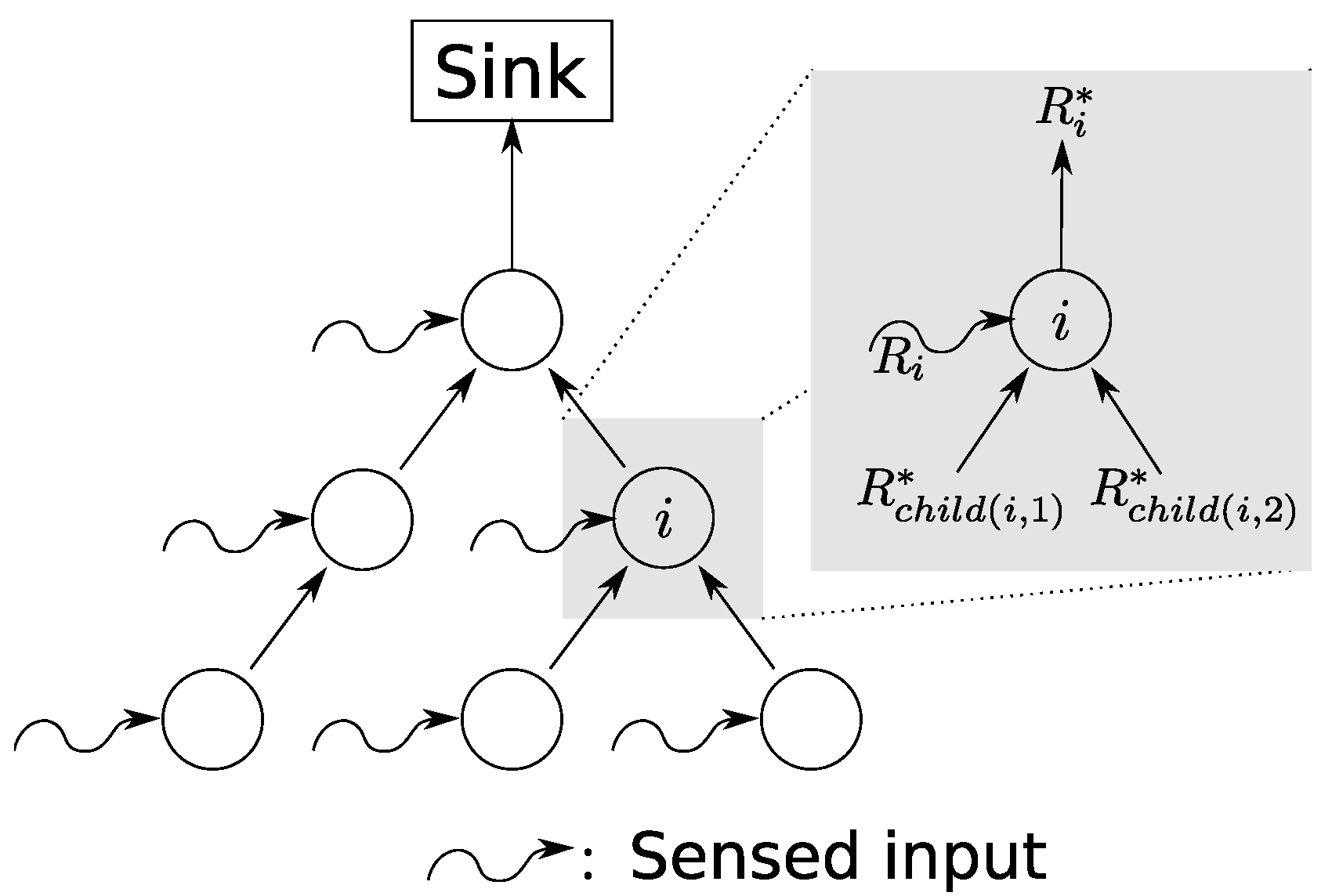
Figure 2.
TDMA service curve.
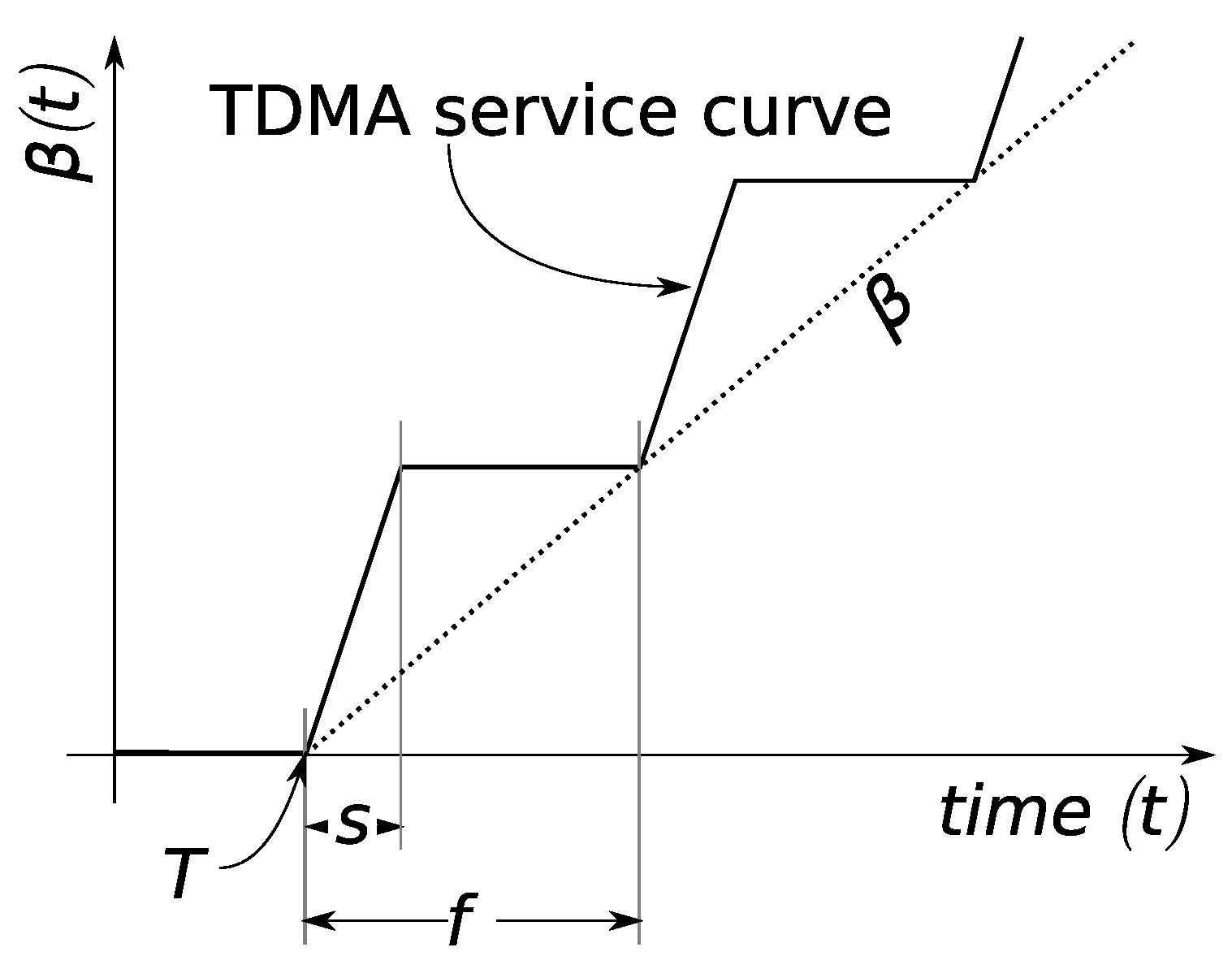
Figure 3.
Simple example to illustrate bounding methods.

Figure 4.
Alternative systems.

Figure 5.
Advanced sensor network model.
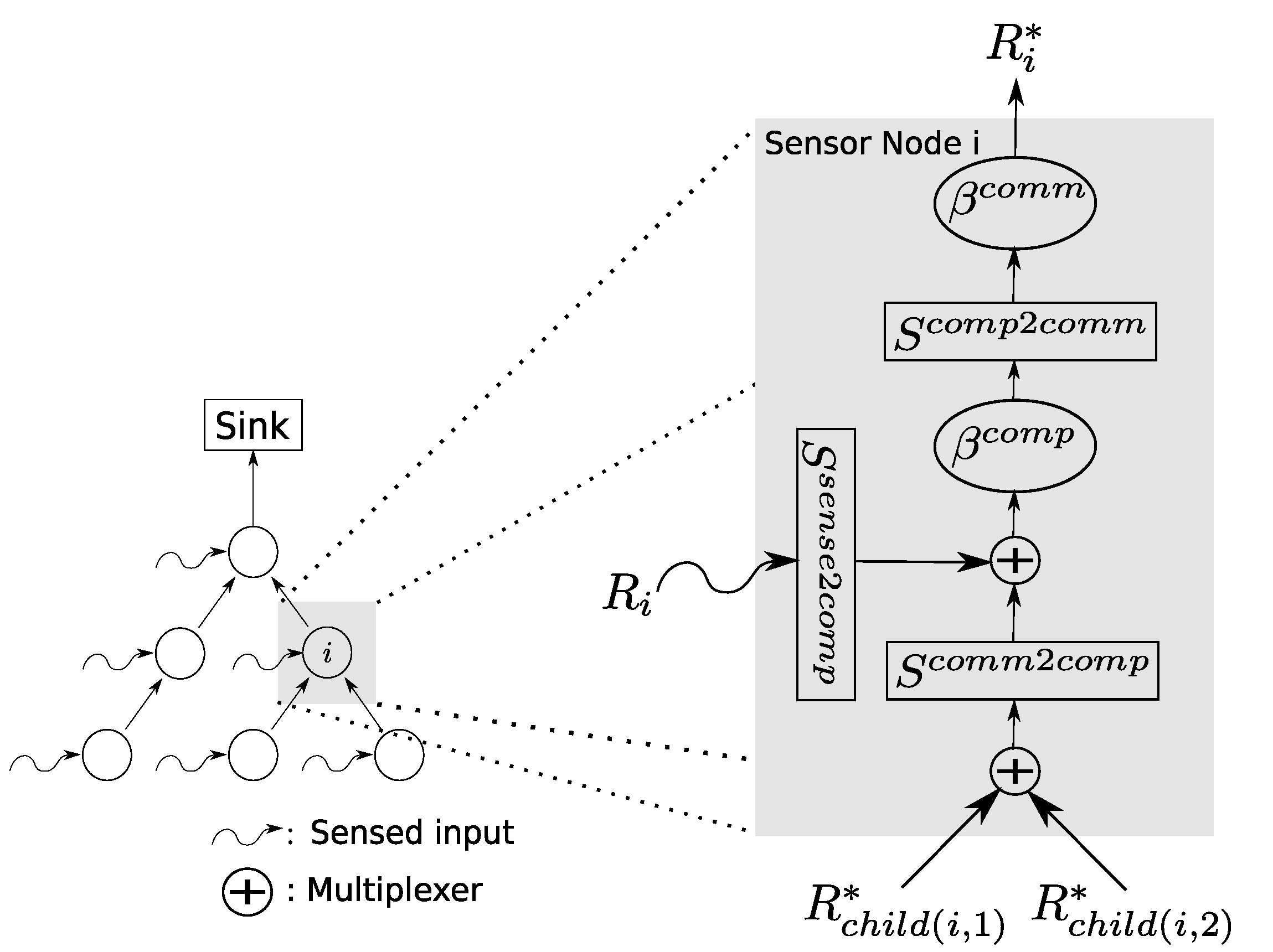
Figure 6.
Scaling element with multiplexer.
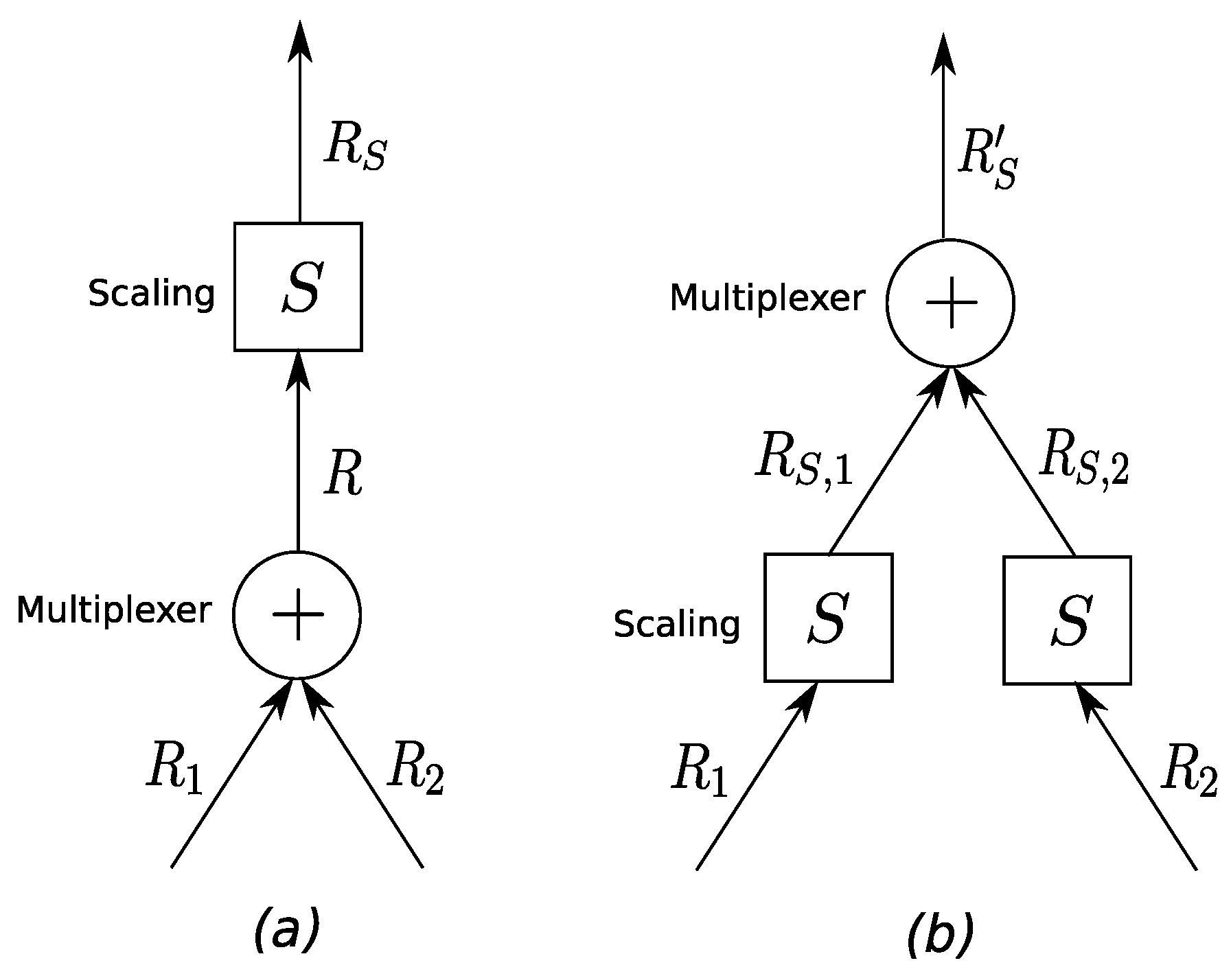
Figure 7.
Baseline comparison between pay multiplexing only once (PMOO) and total flow analysis (TFA) for different scenarios.
Figure 7.
Baseline comparison between pay multiplexing only once (PMOO) and total flow analysis (TFA) for different scenarios.

Figure 8.
Investigation of PMOO vs. TFA under the drifting apart of maximum and minimum scaling curves.
Figure 8.
Investigation of PMOO vs. TFA under the drifting apart of maximum and minimum scaling curves.

Figure 9.
Sink tree network with flow aggregation (left) converted to a set of flow-local views by Theorem 7 (right).
Figure 9.
Sink tree network with flow aggregation (left) converted to a set of flow-local views by Theorem 7 (right).
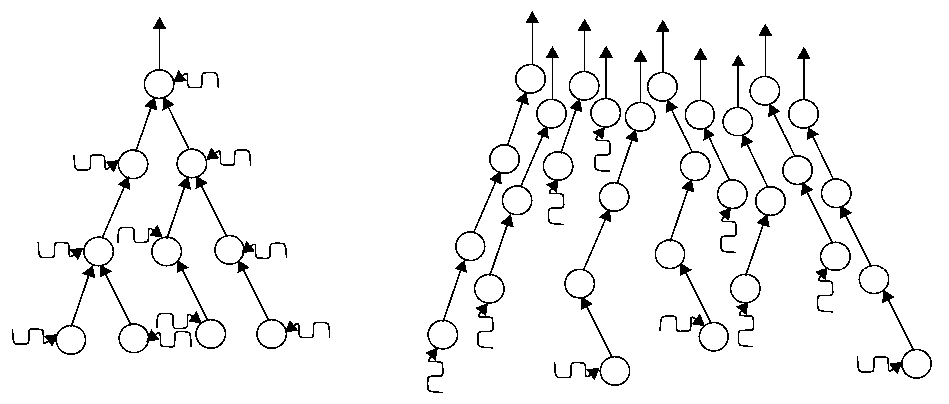
Figure 10.
Generic network calculus computations vs. sensor network calculus (SensorNC): (a) delay bounds and (b) computation time reduction.
Figure 10.
Generic network calculus computations vs. sensor network calculus (SensorNC): (a) delay bounds and (b) computation time reduction.

Figure 11.
The worst case delay comparison of OSP vs. GASP.

Figure 12.
The worst case delay comparison of MCP vs. genetic algorithm-based heuristic for sink placement (GASP).
Figure 12.
The worst case delay comparison of MCP vs. genetic algorithm-based heuristic for sink placement (GASP).
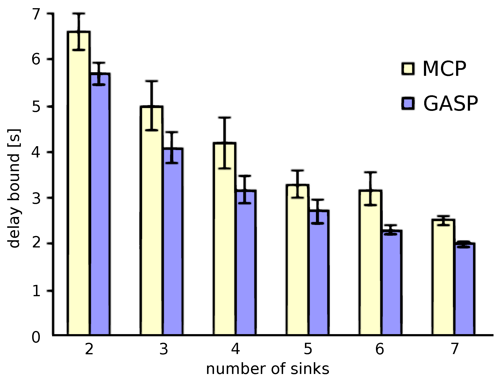
Figure 13.
(a) Random, (b) square grid and (c) tri-hexagon tiling (THT) node placement.

Figure 14.
Worst-case delay comparison of three-node placement strategies in different scenarios.

Figure 15.
Two-node example network.

Figure 16.
Graphical illustration of the optimization problem for Equal slot sizing (ESS). The feasible region is above the delay constraint and below the TDMA integrity constraint. The rate constraint does not affect the feasible region in this example.
Figure 16.
Graphical illustration of the optimization problem for Equal slot sizing (ESS). The feasible region is above the delay constraint and below the TDMA integrity constraint. The rate constraint does not affect the feasible region in this example.

Figure 17.
Flow in a general sink tree.


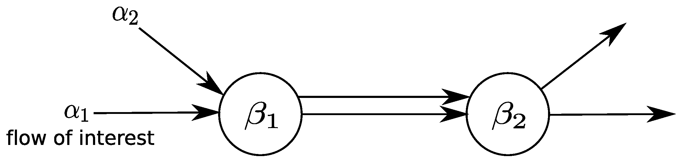
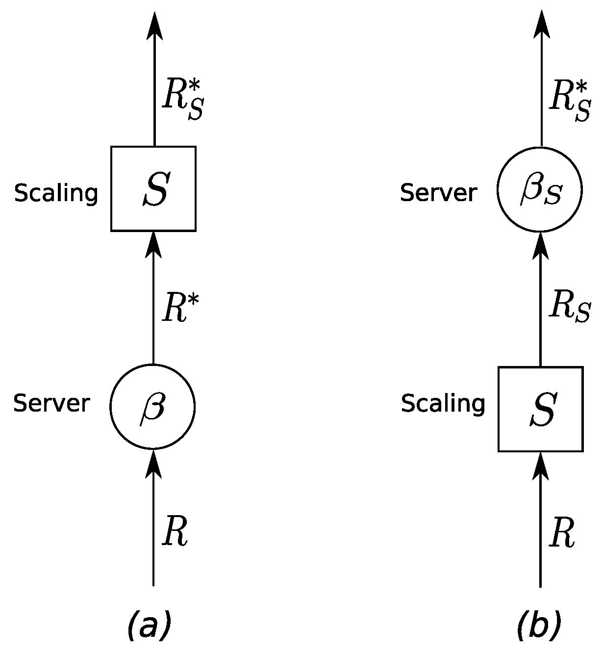
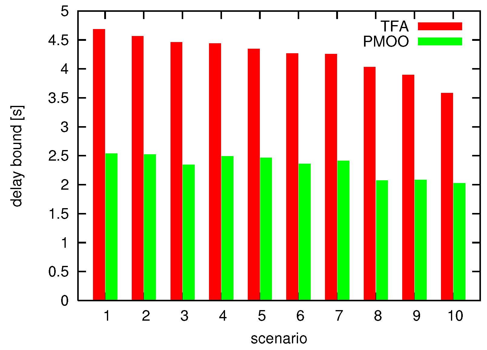
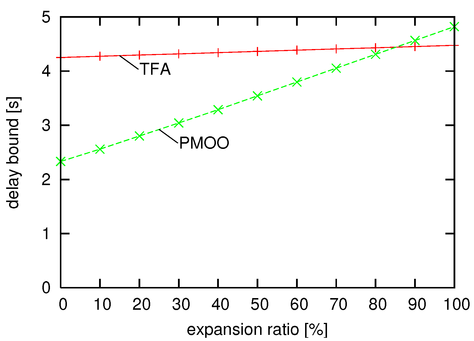
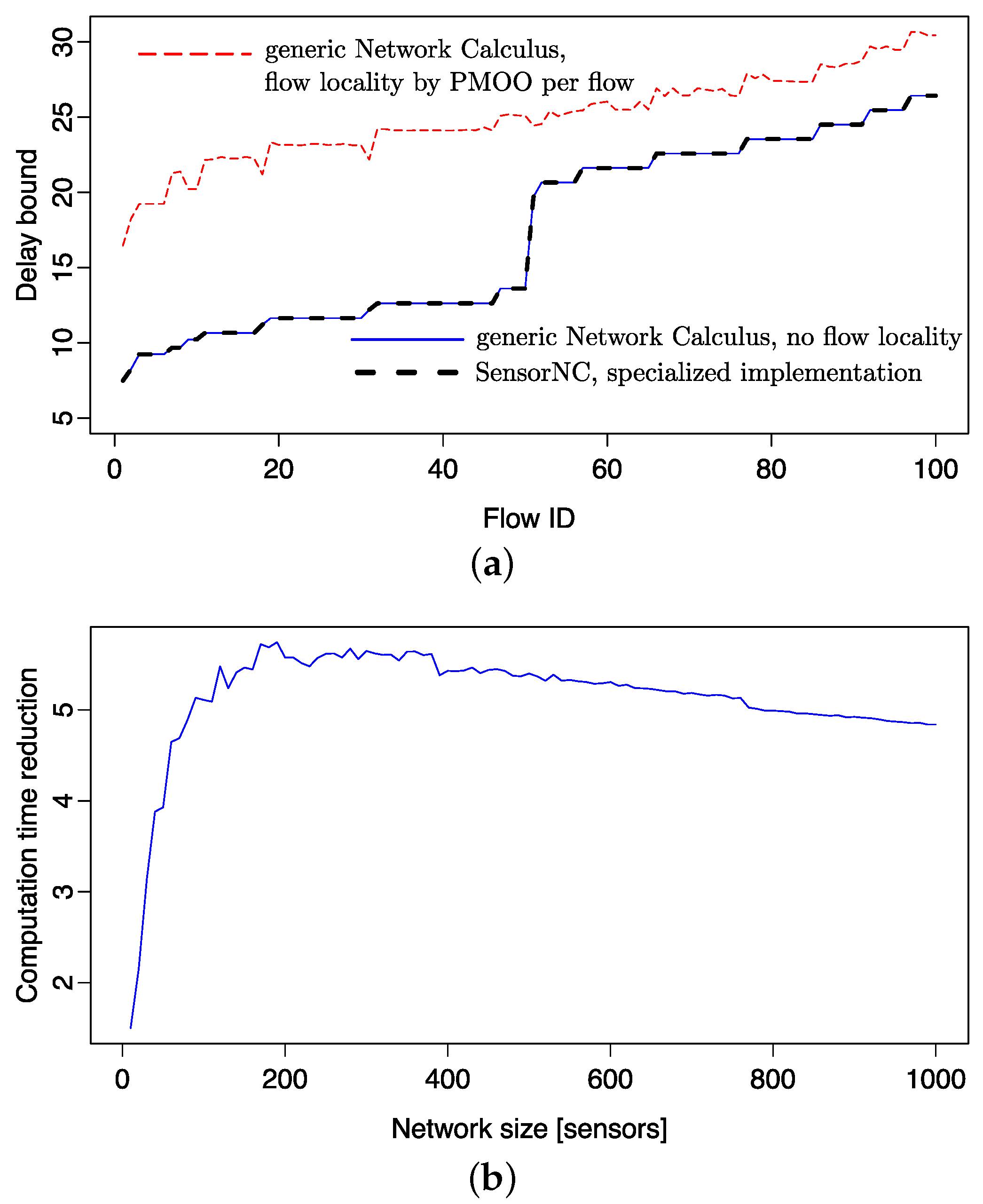
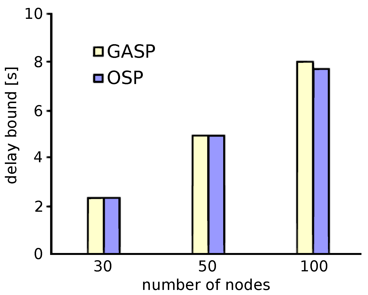
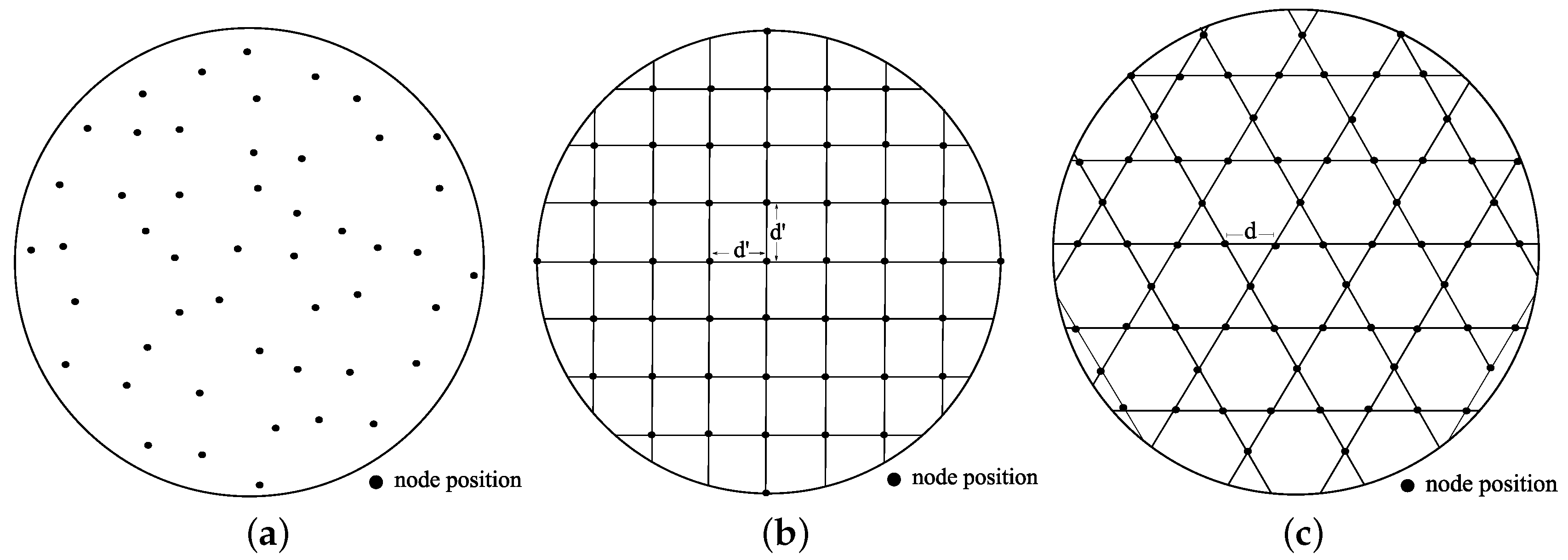
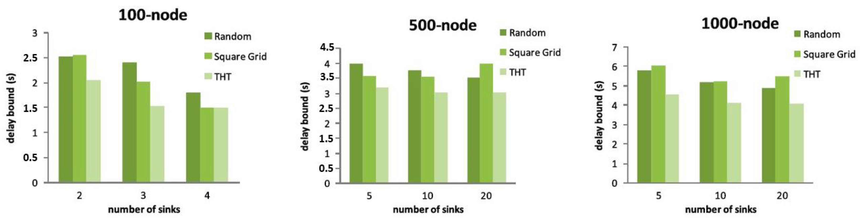
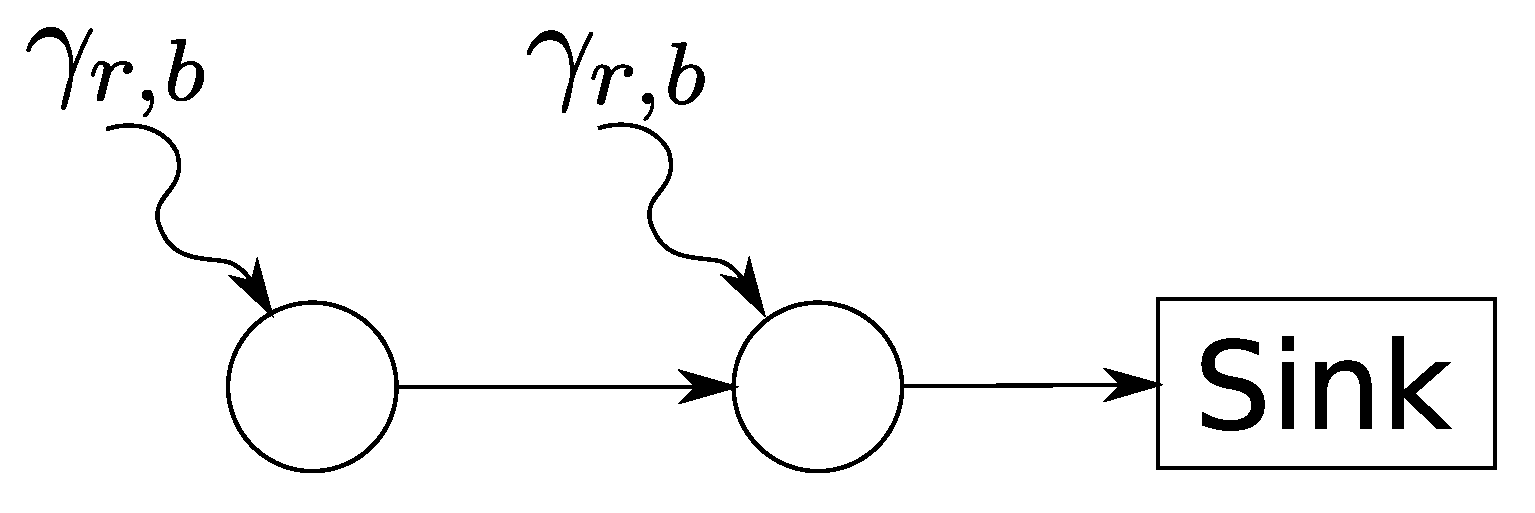
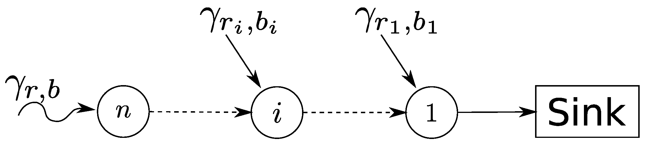
Table 1.
Network calculus notation for functions of arrivals and service, as well as their min-plus algebraic manipulation and performance bounds.
Table 1.
Network calculus notation for functions of arrivals and service, as well as their min-plus algebraic manipulation and performance bounds.
| Quantifier | Definition |
|---|---|
| Non-negative, wide-sense increasing functions passing through the origin | |
| Token-bucket functions with bucket size b and rate r | |
| Rate-latency functions with rate R and latency T | |
| Input function of the flow originating at node i | |
| Aggregate input function for all flows at node i | |
| Aggregate output function for all flows at at node i | |
| , | Arrival curve, arrival curve of flow f |
| Arrival curve of the flow originating at node i | |
| Aggregate arrival curve for all flows at node i | |
| Aggregate output arrival curve for all flows at node i | |
| , | Service curve, service curve of node i |
| , | Left-over service curve, left-over service curve of node i |
| Service curve concatenation with min-plus convolution ⊗ | |
| Output bound computation with (adapted) min-plus deconvolution ⊘ | |
| Left-over service curve computation with non-decreasing subtraction | |
| , | Delay at time t and the time-invariant delay bound at node i |
| , | Backlog at time t and the time-invariant backlog bound at node i |
© 2017 by the authors. Licensee MDPI, Basel, Switzerland. This article is an open access article distributed under the terms and conditions of the Creative Commons Attribution (CC BY) license (http://creativecommons.org/licenses/by/4.0/).
Share and Cite
MDPI and ACS Style
Schmitt, J.; Bondorf, S.; Poe, W.Y. The Sensor Network Calculus as Key to the Design of Wireless Sensor Networks with Predictable Performance. J. Sens. Actuator Netw. 2017, 6, 21. https://doi.org/10.3390/jsan6030021
AMA Style
Schmitt J, Bondorf S, Poe WY. The Sensor Network Calculus as Key to the Design of Wireless Sensor Networks with Predictable Performance. Journal of Sensor and Actuator Networks. 2017; 6(3):21. https://doi.org/10.3390/jsan6030021
Chicago/Turabian StyleSchmitt, Jens, Steffen Bondorf, and Wint Yi Poe. 2017. "The Sensor Network Calculus as Key to the Design of Wireless Sensor Networks with Predictable Performance" Journal of Sensor and Actuator Networks 6, no. 3: 21. https://doi.org/10.3390/jsan6030021
Note that from the first issue of 2016, this journal uses article numbers instead of page numbers. See further details here.