Extended Batches Petri Nets Based System for Road Traffic Management in WSNs †


AMIPS, Mohammadia School of Engineers, Mohammed V University of Rabat, Rabat 10000, Morocco
*
Author to whom correspondence should be addressed.
†
This paper is an extended version of Riouali, Y.; Benhlima, L.; Bah, S. Toward a Global WSN-Based System to manage road traffic. In Proceedings of the International Conference on Future Networks and Distributed Systems, Cambridge, UK, 19–20 July 2017.
J. Sens. Actuator Netw. 2017, 6(4), 30; https://doi.org/10.3390/jsan6040030
Submission received: 1 October 2017
/
Revised: 21 November 2017
/
Accepted: 28 November 2017
/
Published: 4 December 2017
(This article belongs to the Special Issue Sensors and Actuators in Smart Cities)
Abstract
:One of the most critical issues in modern cities is transportation management. Issues that are encountered in this regard, such as traffic congestion, high accidents rates and air pollution etc., have pushed the use of Intelligent Transportation System (ITS) technologies in order to facilitate the traffic management. Seen in this perspective, this paper brings forward a road traffic management system based on wireless sensor networks; it introduces the functional and deployment architecture of the system and focuses on the analysis component that uses a new extension of batches Petri nets for modeling road traffic flow. A real world implementation of visualization and data analysis components were carried out.
1. Introduction
The continous development in highly integrated microelectronics technologies and Information and Communication technology (ICT) have made the wireless sensor networks (WSNs) concept a reality. WSNs, that feature high flexibililty, good scalability and reliability, are emerging as one of the most promising solutions to sense, collect, process and disseminate information from various environmental phenomena. WSN has been widely utilized in various fields including transportation [1], environmental monitoring [2], healthcare [3], battlefield monitoring and surveillance [4], inventory tracking [5], security monitoring [6], civil applications [7,8], and so on. It consists of tiny wireless-capable sensor devices that are battery powered, sense the surrounding environment and have wireless communication, data storage, computation and signal processing capabilities. The data collected from sensor devices is usually sent to a centralized node called sink (or base station) that can act as user interfaces or gateway with other networks [9].
Nowadays, the concept of modern city has emerged to be complex systems that, on one hand invest in human and social capital and in deployment of advanced information and communication technologies, and yet, on the other hand, demand huge quantities of resources and discharge waste into environment [10]; although cities cover only 2.8% of Earth’s surface area, they consume 75% of its global resource and produce an equivalent proportion of waste and pollution that leads to a massive negative impacts [11,12].
The world population has continued to grow rapidly and its concentration in cities keeps rising at an ever-faster pace. It has been projected that the total population in urban areas will jump from 3.6 billion to 6.3 billion by 2050, which means approximatively 67% of the world population. This mass urbanization is bringing with it an inescapable tide of issues such as environment pollution, traffic congestion, energy consumption and inefficient transport systems.
Strictly linked to transportation, one of the most critical issues in modern cities is transportation management. Issues such as traffic congestion and high accidents rate affects environment, economies and human health [13], have pushed the use of Intelligent Transportation System (ITS) technologies in order to facilitate the traffic management or planning to do so in the coming years especially in developing countries [14].
The use of WSNs in Intelligent Transportation System applications such as traffic monitoring and traffic light control has been experiencing a rapid growth [15,16].
Traffic road modeling is a crucial element in traffic management [17,18]. It grows unceasingly clear and has attracted considerable attention of both academic researchers and industry practitioners. There are various criteria for categorizing traffic flow models, according to the level of detail, whether they operate in continuous or discrete time (or even event-based), or whether they are deterministic or stochastic [19,20,21].
Based on the level of detail provided to describe traffic and also the mathematical formulas, Traffic flow can be analyzed macroscopically, microscopically or mesoscopically [22,23]:
Macroscopic models deal with traffic at a high aggregate level. For example, the traffic variables are represented using aggregated characteristics as density, flow rate and velocity.
Microscopic models are based on the explicit consideration of the interactions between individual vehicles within a traffic stream.
Mesoscopic models or kinetic models: The traffic flow is described at an intermediate level of detail. The family of mesoscopic models describes the behavior of individuals in aggregate terms for instance in probability distributions. Thus, traffic is modeled as groups of traffic entities that are governed by flow laws without taking into consideration interactions between individual vehicles.
Petri nets modelling have been approached to study traffic flow at the macroscopic level and we have adopted them as a basis to model the road traffic flow [24].
Petri net are suitable to represent urban traffic systems because they allow representation of states that are distributed, deterministic, concurrent and continuous, and can model shared resources, synchronous and asynchronous communications etc. Moreover, Petri net is a useful formalism for optimizing traffic control and management system. Batch Petri net is an extension of Petri nets; it has been introduced for modelling systems with discrete evolution, continuous evolution and accumulation phenomena. Batch petri nets are proven to be efficient and accurate representation of systems with accumulated continuous elements [25,26]. However, they aren’t able to express accurately all rules and situations in traffic applications such as traffic that has to stop when approaching an intersection and give way rules. We have proposed in [24] an extension of Batch Petri nets that generalize the traffic flow modelling, enable the representation of some complex cases and address the issue of improving energy efficiency in road network monitoring since it involves the minimum number of sensors to capture traffic flow and simulate its evolution over time. To exploit this modelling for managing the traffic dynamicity, we have designed a global system based on wireless sensor networks for achieving energy efficiency during traffic flow monitoring and providing an accurate traffic state estimate and prediction of the overall network. In this paper, we present an overview of the system with its functional architecture and a description of the flow in case of a chosen scenario.
This article is an extended and revised version of our earlier conference paper [27]. The main addition with regard to the conference paper consists in presenting an enhanced architecture of WSN-based traffic management system, and containing additional details about the developed prototype.
The rest of the paper is organized as follow. In Section 2, the related works are reviewed. Our solution, WSN-based traffic management system with its functional architecture and components are described in Section 3 and Section 4 highlights the data analysis component of the proposed WSN based traffic management including the used model for road traffic flow evolution. Details for the deployment architecture as well as prototype of the system analytics and visualization components are reported in Section 5. Section 6 concludes the paper along with description of the intended future work.
2. Related Work
In [28], a scheme that uses a multi-hop replay wireless sensor network (WSN) to monitor urban transport vehicles has been presented and a traffic monitoring system based on WSN that is applicable to all types of city environment was designed. The nodes are distributed dynamically based on the traffic flow forecasts and their statistical law of mobility in order to monitor the important roads that are easily blocked and find out the time changing law of traffic congestion, and then put focus on monitoring them. The paper proposed the use of gray model in order to forecast the traffic flow. Gray model is simple and doesn’t require a huge amount of available data like many other methods. However, one of its disadvantages is that it cannot deal with non-linear structure of data which decreases its efficiency and competitiveness in forecasting road traffic flow on complex networks.
A wireless sensor network based monitoring system has been proposed in [29] with dynamic mathematical model for managing road traffic in important intersections of a city. It aims at reducing congestion by broadcasting the traffic status when it comes to a congested status. Monitoring and calculating the congestion level on the most important intersections is not always a relieable approach since too many cars on intersections is only one reason of traffic congestion. Other causes such as double parking and events that may change traffic dynamics at any place within roads are not taking into consideration.
Nafi et al. [30] presents a Vehicular Ad-hoc Network (VANET) based predictive road traffic management system (PRTMS). PRTMS is simple and uses a modified linear prediction algorithm to estimate traffic intensities at different intersections using a vehicle to infrastructure (V2I) scheme. However, the proposed system architecture, which relies mainly on information received from vehicles and V2I communications requires a significant power resources.
In [31], A traffic congestion detection system was presented that combines vehicle-to-vehicle (V2V), vehicle to infrastructure and infrastructure-to-infrastructure (I2I) connectivity and big data. The system aims at decreasing travel time and reducing CO emissions by allowing drivers to identify traffic jam and change accordingly their routes. The proposed system monitors, processes and stores large amounts of data into a Cassandra table which is one of the open-source distributed NoSQL databases. Through a series of algorithms, a big data cluster identifies vehicular congestion and informs drivers so that they can make real time decisions and avoid it. A weakness of this work is that the system cannot answer queries. For instance, it cannot evaluate the impact of upcoming events such as road works on traffic flow state.
Iwasaki et al. [32] proposed a method for stop line detection using thermal images taken with infrared cameras under different weather conditions. According to the first method, the windshield of a vehicle and its surroundings are used as the target of pattern recognition. The vehicle detection process involves spatio-temporal image processing by computing standard deviations of pixel values, vehicle pattern recognition by using Viola-Jones detector [33,34] that considers the windshield and its surroundings as the target of pattern recognition, and correction procedures for misrecognized vehicles.
Since the vehicle detection accuracy decreases in low temperatures because the temperature of the windshield is usually similar to that of the windshield exterior, Iwasaki et al. proposed a second method, to deal with this limitation, that detects vehicles based on tire thermal energy reflection area on the road surface. The method is based on the idea that the temperature difference between the tires and the road surface is considerably high in cold weather. By combining both methods, the overall vehicle detection accuracy was highly maintained under various environmental conditions and an automatic traffic flow monitoring was achieved by computing the number of vehicles in the target area and the degree of movement of each vehicle.
Another approach proposed in [35] uses vehicles as mobile sensors for sensing the urban traffic and send the reports to a traffic-monitoring center (TMC) for traffic estimation. The so-called probe vehicles (PVs), i.e., taxis and buses that are equipped with the necessary devices to transmit traffic conditions to the TMC at regular time intervals, and floating cars (FCs), such as patrol cars for surveillance, report periodically their speed and location to traffic-monitoring center.
Since PVs cannot cover all roads in most of the time, a Matrix Completion (MC) has been proposed to reconstruct data in empty rows in the collected probe data. In order to facilitate MC based estimation and improve its performance, Du et al. proposed a floating car control algorithms. However, the proposed approach doesn’t take into account different sources of traffic data and correlation of road sections.
Based on the previous studies and literature reviews, the challenge of designing a monitoring energy-efficiency system while ensuring the accuracy of traffic flow estimation and prediction remains open.
The system we propose aims at enabling energy-efficient management and providing accurate estimation and prediction of road traffic by:
- Modelling the traffic in order to predict its evolution in accordance with deploying of the minimum number of sensors.
- Estimating vehicles dispatched in a road intersection using statistical models
- Taking into account events for predicting traffic status
3. WSN-Based Traffic Management System (WTMS)
In this section we present functional architecture of our management system. The system takes advantage of WSNs technology, traffic modelling and data learning approaches for dealing with traffic-related challenges and leading to more efficient and safer travels. Before turning to this discussion we introduce an overview of the system.
3.1. Overview of the WTMS
The proposed road traffic management system aims to monitor the road network and proactively provide information about traffic flow. It takes input from various sources, mainly road sensors, and internet to ingest weather and events information such as national celebrations, sportive events (soccer games etc.). Data afforded from vehicles, especially neighboring traffic flow and average speed, can be included in the system’s input in order to refine better the output and the final model, and then model the road network and the traffic flow dynamics spatially as well as temporally, and yield to an overall traffic flow of road network.
This allows the cars, buses, taxis to respond to the city’s needs on the fly.
Raw data always goes through at least one filter before being delivered to models and estimation algorithms. The output of these models is used in various applications such as adaptive traffic signal control and dynamic route guidance and is sent to third parties for consumption or analysis. Consequently, reliable information can be shareable with the public over internet. For instance, the road users can be informed of the traffic congestion and real time traffic situations through mobile applications.
In the following section we briefly describe the WTMS through its components.
3.2. WTMS Architecture
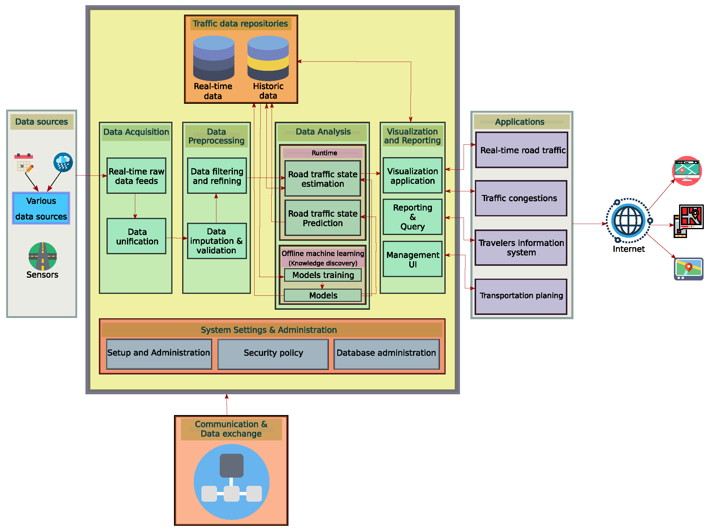
Our WSN-based Traffic Management System is composed of several components which are: Data Acquisition, Data Preprocessing, Data analysis, Visualization and Reports, System Settings and Administration, Traffic data repositories and finally Applications. All these components use Data Communication component. Figure 1 illustrates the functional architecture of the system. In the next, we describe each component.
3.2.1. Acquisition Component
Data acquisition consists of gathering the raw data and passing it to data preprocessing component. The data can be acquired in different formats and it draws from heterogeneous sources. This component has to ingest all needed information that will be sent to the other components in a unified format. Data acquisition contains two subcomponents:
Real-time raw data feeds
Real time data feeds are collected through sensors. This data includes traffic volume, average speed, roadway conditions. This part of system has to deal with two approaches of data acquisition:
- Pull-based approach: it allows users to selectively acquire and query the data at preferred point in time, within a specific time interval or within a user-defined frequency acquisition.
- Push-based approach: In this approach, data acquisition is executed in regular periods. Data are disseminated proactively through sensors, i.e., the sensors can decide when to send data to a centre node such as a sink.
Adding to roadside sensors, other sources of data can be taken into consideration such as vehicles, especially regarding the movement count estimates, and traffic.
Data unification
Data unification means the integration of data culled from raw sensor data and a variety of other structured of unstructred sources such as scheduled events, weather information, road works etc. and the representation of this heterogeneous data in the same unified format.
3.2.2. Data Preprocessing
This component is responsible for the preparation of raw data for further utilisation and providing the cleaned data; the collected data must undergo a preprocessing step where it must be checked, filtered and completed in order to avoid as much noise as possible and being usable by models. Data preprocessing includes:
Data filtering and refining
Data in real-world contain redundant information. Data filtering and refining is the process of cleaning data by filtering duplications, data that contradicts itself and noise and ensuring data integrity. This is essential for obtaining consistent modeling results.
Data imputation and validation
Due to sensors malfunction, measurements can be erroneous, missed or corrupted. Therefore, some preliminary tasks need to be performed for effeciently analyzing the data such as data imputation and data validation. In this step, imputing missing values and examining data quality and reliability are performed.
3.2.3. Data Analysis
Data analysis aims at turning recieved data into information that guides effective decision making through estimating the current traffic state and traffic flow dynamics evolution over time and space. To this end, Data analysis has two aspects: offline machine learning for knowledge discovery and runtime compenents for applying the knowledge during the execution.
Offline machine learning includes:
Models training
This component carries out the necessary machine learning tools to train models based on new data.
Models
It consists of mathematical equations and parameters that are trained and calibrated, but are improved using additional knowledge.
The runtime part is composed of road traffic state estimation and road traffic state prediction:
Road traffic state estimation
It is the most mandatory component of the system since it transforms multisource traffic data into useful traffic information and provides the basis for additional application and practices. In this subcomponent, we use the generalized nondeterministic batch Petri net formalism to model the road traffic for each segment in one hand. In another hand, the necessary models, when needed, are deployed and executed.
Road traffic state prediction
Given historical information, or driving correlation and dependencies among the road network, this module is performing short and long-term predictions using models that were built offline. We aim at predicting traffic flow from few minutes to several hours ahead.
3.2.4. Visualization and Reports
The output of models can be used for further analysis. Converting models results into well-formed forms for analysis, visualization or end-user information is a real benefit from data analysis component. This can simply enhance decision making. In addition, analyzed data and reports can help traffic planner to make well-informed decisions and interact fast to different traffic situations and evaluate or design transportation facilities. Or on another side, it can enhance the individual traffic participants’ navigation.
Visualization applications refer to a web-based tool that provides a holistic view of the overall road network while displaying the emergency events as well such as congestion. Reporting and Query refers to tools that offers traffic reports for advising travelers and traffic managers and planners and allows users to interactively query up-to-date information. Management UI is a set of user interfaces for that enables traffic planners and managers to set up traffic and roads parameters such as road length, maximum velocity and traffic signal cycle lengths and to enhance their interventions through broadcasting notifications and alerts to travelers.
3.2.5. System Settings and Administration
System settings and administration component handles prepares the sensor infrastructure, it allows configuration of sensor data, that are needed for applications, and intervals. It allows displaying and modifying all configurations. This includes security policies, user roles and database administration.
3.2.6. Traffic Data Repositories
It supports the storing of raw traffic data and archiving of historical data for use as needed. The stored data concerns the data aggregated from sensors, the necessary data structure for modelling the traffic flow, the historical data to train the machine learning or statistical models to achieve prediction, etc.
3.2.7. Communication and Data Exchange
This allows the network to communicate the traffic information and exchange data between its various components.
In the next section we will focus on the data analysis component and more precisely on generalized nondeterministic batch Petri net model that we adopt for this system.
4. Road Traffic State Estimation
Road traffic flow is a very complex phenomenon. To approach its dynamic evolution we proposed the generalized nondeterministic batch Petri net [24] since it deals with both continuous and discrete states that characterize traffic flow and allows modeling its behavior along roads for complex cases.
4.1. Background on Triangular Batches Petri Net
In this section, we introduce Petri nets concepts and the theoretical background of our extension of batches Petri nets model.
4.1.1. Petri Nets
In his PhD Thesis, Carl Adam Petri introduced Petri nets in order to represent the global state of a system as composed of a set of local states [36]. Petri nets are both a graphical and mathematical tool for design, modeling and formal analysis of various discrete event systems [37]. Being a graphical tool, it allows to easily represent the different interactions in a complex system such as concurrency, parallelism, synchronization, non-determinism, communication, alternatives and so on by means of only few elements types. Being a mathematical tool, it allows to fomally model these interactions and analyze the properties of the modeled system [38].
A Petri net can be defined as a directed graph that consists of two types of nodes interpreted as places and transitions where an arc can only connect two nodes of different types [39]. Places are drawn as round shapes (circles or eclipses) to model different states of a system. Transitions are depicted as rectangular shapes (rectangles or bars) to represent events or activities that can cause the change of a system state. An arc connects a place to a transition or vice versa, it models the flow of processes through the system and the abstract relationship between a place and a transition. The dynamic behavior of a system is introduced by means of tokens into places where every place holds either zero or more tokens that are graphically appear as solid dots in places. At any given time, the distribution of tokens among the places, termed Petri net marking, determines the current state of the modeled system. A marked Petri net consequently is used to study dynamic behavior of the modeled system.
Formally, a Petri net is quadruplet where:
- -
- P and T are, respectively, disjoint non-empty finite sets of places and transitions;
- -
- : is the backward incidence matrix, : is the forward incidence matrix.
Over the years, several extensions of the original Petri net model have been developed, we mention in the following paragraph some of them in order to better understand the proposed model in this paper.
4.1.2. Generalized Batch Petri Nets
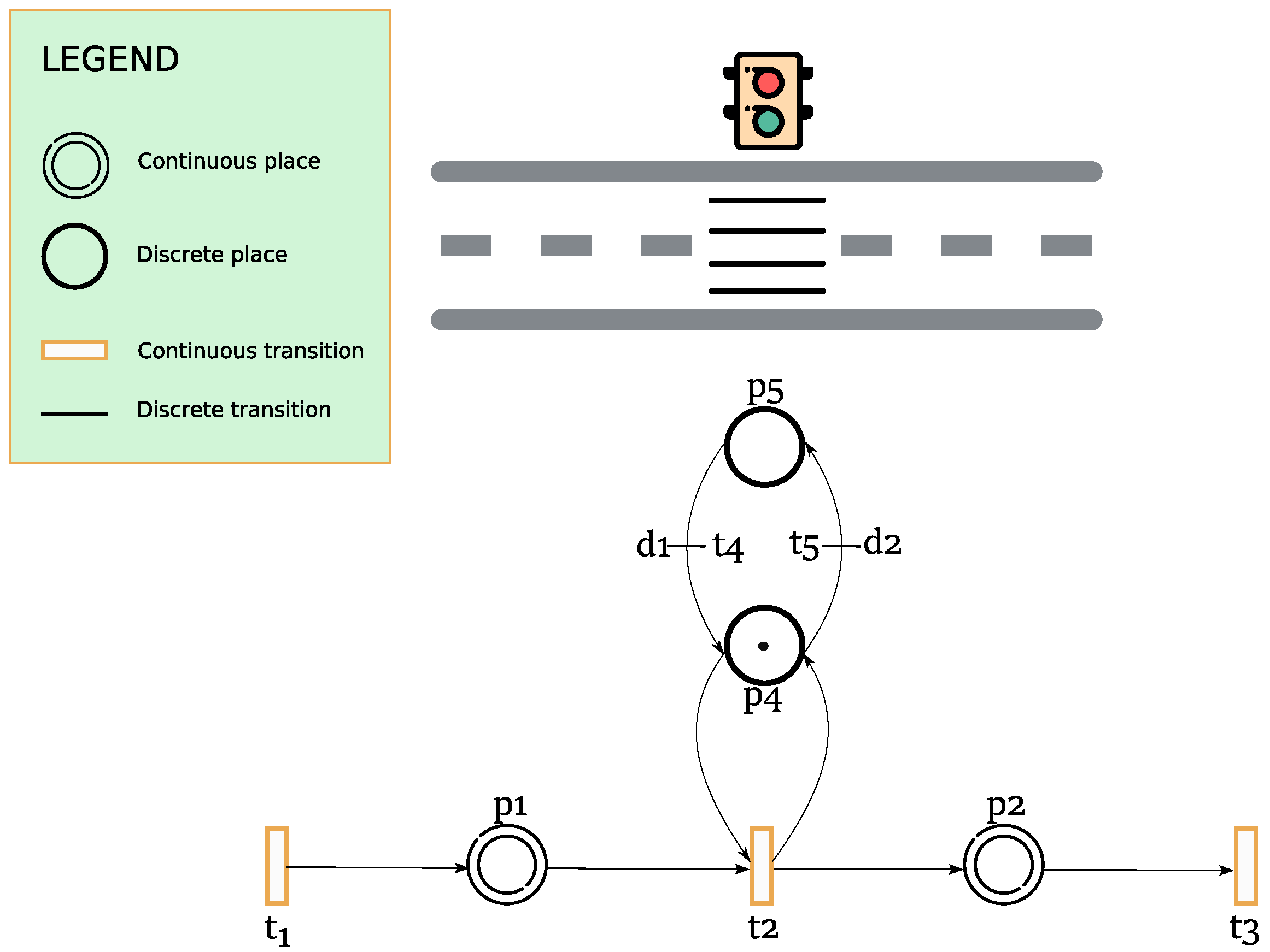
Hybrid Petri nets (HPN) contain two parts: a discrete part and a continuous part since they include discrete and continuous places and transitions. For instance, in traffic system, traffic lights are modeled as discrete places and transitions and road sections can be modeled by continuous places as can be illustrated in Figure 2.
Figure 2 shows an example of signalized street with its HPN model where is the set of continuous places representing the two sections of the road, is the set of discrete places that models the signal system switching between red and green. is the set of continuous transitions model the limit between two sections and is the set of the discrete transitions which represent the delay associated with every section for switching between green and red lights.
Batches Petri nets are a modeling tool for systems with accumulation. The new with this extension of HPN is the introduction of batch concept; a batch is a group of entities whose movement through a transfer zone (i.e., a portion of road), and is characterized by continuous variables, namely the length, the density, and the head position. Thus, batch places represent the delays on continuous flow and batch transitions behave like continuous transitions are associated with a maximum flow.
4.1.3. The Triangular Batches Petri Net
In the following, some of the main definitions of triangular batches Petri nets are presented.
Definition 1.
The triangular batches Petri net can be defined by the following elements:
A triangular batch Petri net is whereP is a non-empty finite set of places partitioned into discrete , continuous and batch places : ; Continuous places are used to model variables real values; While discrete places are used in modelling variables with integer values; Batch Places are used to model transfer zones whose elements move at the same speed.
T is a non-empty finite set of transitions partitioned into discrete , continuous and batch transitions .
, respectively : are defining the we ight of arcs directed from places to transitions and the weight of arcs directed from transitions to places.
is the batch place function. It associates with each batch place the of continuous characteristics that represents, respectively, a speed, a maximum density, a length and a maximum flow.
Time: it represents the firing delay in case of discrete transitions and the maximal firing flow in case of continuous or batches transitions.
For analysis of Petri net, two notions are needed: Preset and Postset since they are crucial in modelling, respectively, pre-conditions and post-conditions of a system changes.
Definition 2 (Preset and Postset).
Let and be the number of places and transitions in a TrBPN, respectively. The preset of a place p (resp. of a transition t) is defined as (resp. ) and the postset is defined as (resp. ).
Batches are moving at different speeds. For controlling this, the concept of controllable batch is introduced.
Definition 3 (Controllable batch).
Additionally to the three basic characteristics of a batch, a controllable batch is characterized also by the speed. . An instantaneous batch flow of is given by: .
The marking of the batch place is a series of batches ordered by their head positions.
The moving of batches and their evolution depend on the state of batch places and are governed by various functions, namely: Creation, Destruction, Merging and splitting.
Definition 4 (Dynamics of controllable batches).
For every batch place, four continuous dynamic functions can change the values of its batches and then change its marking.
Creation: A controllable batch , is created inside a batch place and added to its marking if its input flow is not null i.e., With
Destruction: A controllable batch is destroyed, if its length is null i.e., and it is not a created batch i.e., , such that and removed from the marking.
Merging: A controllable batch is obtained from the fusion of two batched, if they are in contact with the same density and the same speed. Consider the two controllable batches: and with , and , becomes and is destroyed .
Splitting: A controllable can be split into two batches in contact with same density and the same speed.
The aforementioned models aren’t able to express accurately some rules and situations in traffic applications such as priority roads, traffic that has to stop when approaching an intersection. For example, the traffic behavior can change significantly due to the type of intersections whether they are right-of-way or roundabout, the presence of road signs or not. Therefore, taking into consideration non deterministic time based traffic dynamics will lead to improve modelling accuracy and generalization.
4.2. Our Extension: Generalized Nondeterministic Batch Petri Net
The batch Petri net that will be presented in this section is based mainly on the same principles as triangular batch Petri net such as triangular fundamental diagram, generalizes the traffic flow modelling and tackles other cases of road networks. We extend the existing formalization to support, on one hand, dependencies between traffic flow dynamics and external conditions, and on the other hand, events that change dynamics at any place within roads.
To illustrate this, consider the following example:
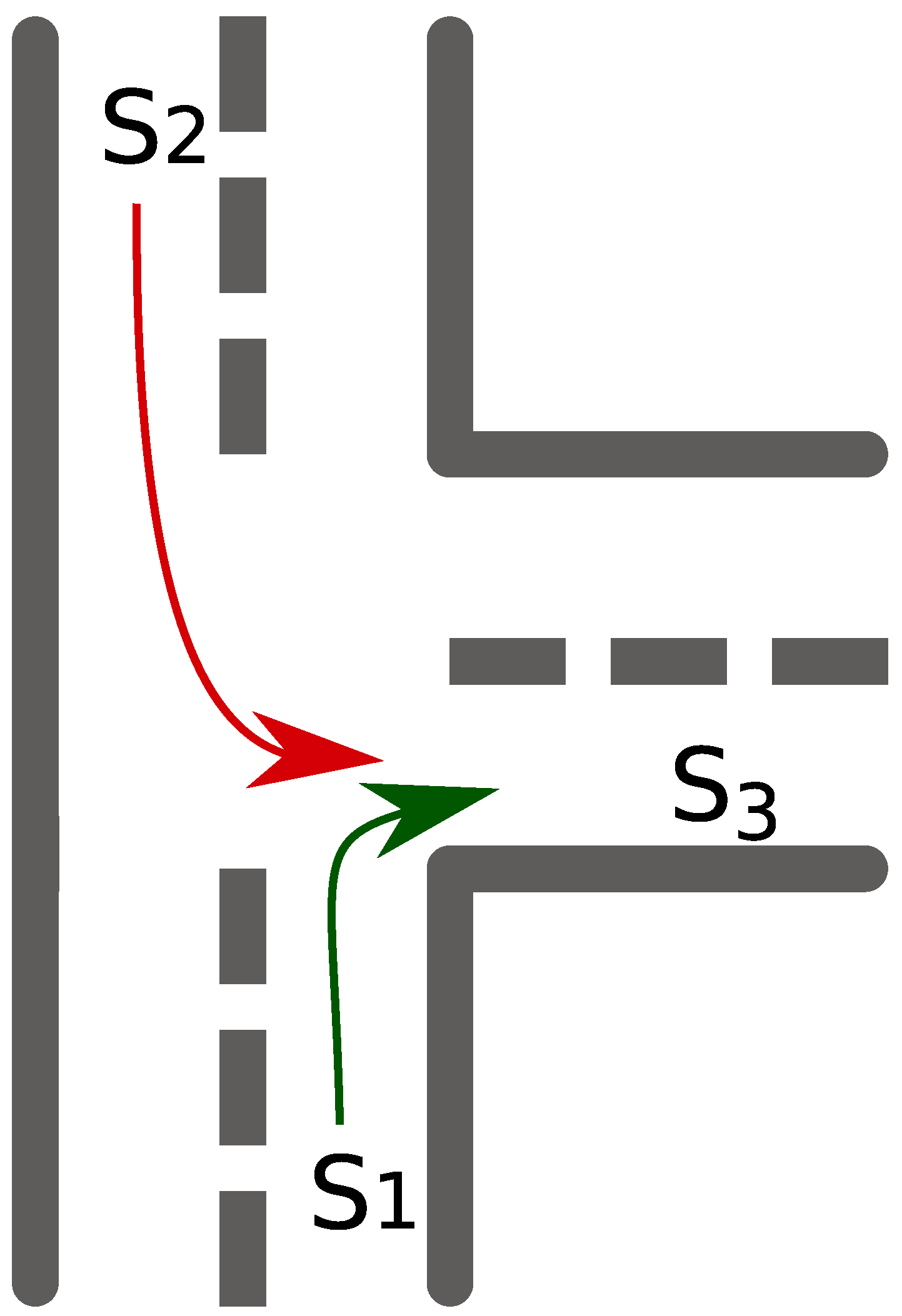
Example 1.
At T-intersection, the batch coming from section and aiming to turn left, it must give way to the oncoming batch from section . Figure 3 illustrates this giving way case.
By considering the above example and other such situations, the traffic behavior or the batch is not only depending on simple delay times or flow rules but can also depend on more complex uncontrollable events that may even change completely the batch characteristics. In the triangular batches Petri net modeling, these cases and others are not modeled precisely or are not considered; For instance, in the example mentioned above, the batch (coming from ) doesn’t have necessary the same behavior since the batch can be divided according to the other traffic behaviors (batch coming from ); the condition that has to be filled is neither delay time nor flow rule, the traffic has to stop and wait for the way to be clear.
The proposed generalized nondeterministic batch Petri net (GNBPN) seeks to complete Petri net formalism by adding new non-deterministic time based transitions which we call untimed transition in order to formally represent changes that depend on external conditions (i.e., vehicles move at intersections only when the road ahead is empty). This allows us to include uncontrollable events which cannot be fixed in time. Moreover, we enrich the model to take into consideration relationships to previous observed changes at a given station and/or to neighboring roads at the same time; for instance, at fork, splitting a traffic flow into more accurate proportions can depend on temporal and spatial information (presence of an event, roadworks, etc.). The benefit of the added statistical feature is to enhance the firing rule of batch transitions.
Generalized nondeterministic batch Petri net (GNBPN) is defined formally as follows [24]: Where:
- P, and are respectively the set of places, the pre-incidence and the post-incidence matrices;
- T is a finite set of transitions that are partitioned into the three set of timed , untimed and batch transitions ;
- C is the “characteristic function”. It associates with every batch place three continuous characteristics that represent respectively speed, maximum density, and length and the total number of segments of the batch place;
- f: is an application that associates a non-negative number to every transition:
- if , then denotes the firing delay associated with the timed transition expressed in time unit;
- if , then denotes the maximal firing flow associated with the batch transition expressed in entities/time unit and estimated by statistical models in case of multiple outputs;We use the symbol f to refer to firing rules of transitions which can depend on both delay times and flow rules.
- is the priority of a transition according to the output flow of a place, . This priority’s feature is added to support non-deterministic time based transitions.
For better understanding of the concept of GNBPN model, we illustrate the primitives of the proposal petri net using the example of T-intersection where the batch, coming from section and aiming to turn left, must give way to the oncoming batch from section (Figure 3). The Sections and are represented respectively, by batch places , . The intersection is modelled by the batch place . While the maximum inputs flow of and are modelled by the batch transitions and .
The give way rule within intersection is modelled by the untimed transition representing that vehicles at section have to wait until the traffic ahead clears the intersection. Maximum flows , and of batch transitions , and represent, respectively, the maximum output flow of Sections and and the maximum input flow of section . The associated model is shown in Figure 4.
5. Implementation
This section presents a deployment architecture that uses wireless sensor network and then it introduces an implementation of Visualization component and Traffic Modelling and Analytics component of the WTSM.
5.1. Deployment Architecture of WTMS
All nodes in this network are connected directly to a base station or via a relay node if needed and share their data. On another hand base stations model the traffic flow based on the received data and then output the current traffic flow state. Consequently, they send the estimated traffic flow to the Control manager that evaluates all the received traffic flow estimations and provides an overall traffic estimation for the network. Such that, if congestion is detected, the Control manager broadcasts an alarm notification to the authorities in order to take appropriate decision. The system deployment architecture is illustrated in Figure 5.
The proposed system is mainly made up of the following elements:
- Sensor nodes: are responsible for detecting traffic flow at points of interest namely the beginning of roads, and sending the real time measurements to the sensor head;
- Relay nodes: are intermediate sensor nodes that are used in case the network is wide and a multi-hope communication is needed;
- Sensor head: The duty of the sensor head is to aggregate the physical traffic parameters that were captured by sensor nodes like density, velocity and to send the aggregated data to the base station.
- Base station: The major purpose of base stations is to model and simulate the received traffic flow in the corresponding region and provide its dynamic evolution over time.
- Control manager: provides more coherent traffic flow of the overall road network, while dealing with some of the most common critical situations such as congestion.
Following is a simple use case representing the WSN based traffic management system and how it can operate when detecting traffic flow in road network.
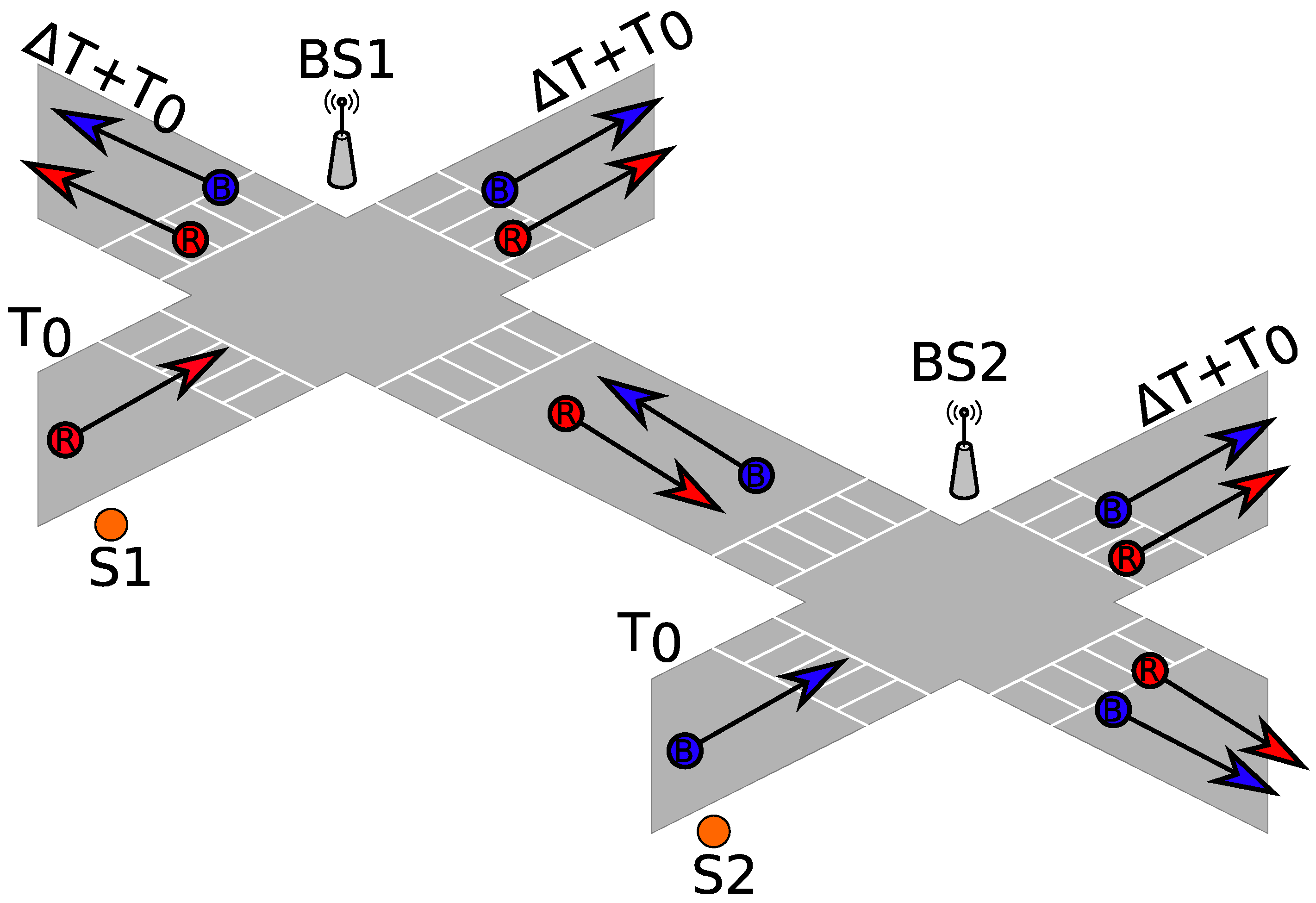
The scenario consists of two intersections and where two roads cross each other as depicted in (Figure 6). At least two sensors are positioned preceding every road to detect and transmit the data that consist mainly of velocity, density and length of the entering vehicles. These data are collected in the base station so as to model the traffic flow and estimate its evolution within the network.
Suppose at time , different batches of vehicles are detected within roads and (Arrows blue and red) by a set of sensors that are positioned at the beginning of these roads. Sensor S1 will transmit information about velocity, length and density to the corresponding base station , through the sensor head, where generalized nondeterministic batch Petri modeling will perform and output the traffic flow evolution at every section of roads i.e., the velocity, the length, the density and the time when vehicles will be there. The same process will be carried out for sensor 2 and . Consequently, a control manager will model the whole network based on the output of every base station.
5.2. Prototyping
A prototype has been developed in order to implement the data analysis component and more precisely the proposed GNBPN model and check its applicability. To this end, we have proposed a preliminary architecture consisting of the following elements: Web interface, two sensors and a base station.
The web interface is meant to allow the system administrator to save the characterestics of each road within the network mainly its maximum speed, maximum density and length.
The sensors are meant to detect a batch of vehicles and determine its average speed and density.
The base station is meant to execute the batch evolution model GNBPN based on the inserted parameters through the web interface and the detected values received from sensors.
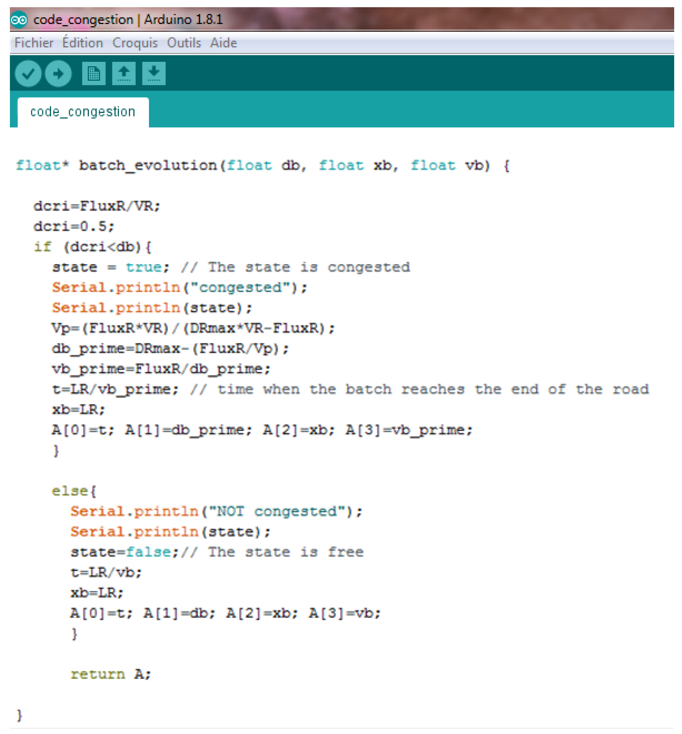
The suggested prototype aims mainly at implementing a simplified version of GNBPN model. This simplified version is used to study the dynamic evolution of a vehicles batch that is moving in a certain section of the road, in order to predict whether congestion may occur at the level of the entire road or not.
To perform the calculations necessary to determine the vehicles batch evolution within a section, the algorithm takes as inputs:
- The characteristics of the vehicles batch, which are:
- -
- : The density of vehicles batch (veh/km);
- -
- : The position of vehicles batch;
- -
- : The speed of vehicles batch (km/h).
- The characteristics of the road R:
- -
- : The length of the road (km);
- -
- : The maximum density (veh/km);
- -
- : The maximum speed (km/h);
- -
- : The maximum flow (veh/h).
Once the algorithm is executed, it yields the output vector A which contains four values describing the evolution of the batch, namely:
- t: The travel time needed to reach the end of the road;
- : The updated density of vehicles batch;
- : The updated position of vehicles batch;
- : The updated speed of vehicles batch.
Figure 7 shows the Arduino IDE with a sample of the simplified sketches loaded.
The development of the prototype involved the use of two HC-SR04 ultrasonic sensors for detecting the vehicles batch and sending the measurements to the base station, a MAMP Web Server and an Intel Galileo Gen 2; the intel Galileo Gen 2 development board is used as a base station on the one hand, and as data aggregation platform on the other hand. This board plays the role of sensor head since it performs an aggregation operation over sensor measurements such as aggregating vehicles speed. Also, Intel Galileo Board performs the simplified version of Batches Petri nets algorithm using the aggregated data and the input parameters, that were given through the web interface, to determine whether a congestion will occur or no. Figure 8a shows the used Intel Galileo Gen 2 connected to two HC-SR04 ultrasonic sensors.
The current deployed version of the model is totally based on installation on Galileo gen 2 boards. The software installation process consists of the following steps:
- -
- Setting up the computer for development with the Galileo Gen 2 board by installing arduino integrated development environment (IDE) software;
- -
- Writing and Uploading the code: Once the code is created, it has to be compiled and uploaded to the Galileo board.
The system contains a web interface as well for inserting the required parameters for the model such as maximum density, maximum speed and maximum length of a road.
Figure 8b shows the web interface screen. The data inserted is thus sent and stored into a XAMPP based database server.
In this work, the HC-SR04 ultrasonic sensors have been chosen to detect vehicles batch and measure its speed and density. They operate on 5 V and provide 2 to 400 cm or 1” to 10 feet non-contact measurement function with high accuracy and stable readings (up to 3 mm accuracy).
The HC-SR04 ultrasonic sensors consist of a transmitter and a receiver. The transducer transmits eight 40 kHz pulses of ultrasonic pulses which travel through the air until it meets an object that these pulses are reflected back by the object. The waves reflected by the objects and received by the transducer are used to compute the speed and density of vehicles’ batch by Intel Galileo Gen 2.
Intel Galileo Gen 2 Development board is powered by intel Quark System-on-Chip (SoC) ×1000 and operating at speed up to 400 MHz. it runs on an embedded Linux Kernel and it ensures saving data on the SD card and transmitting them using internet.
The advantage of using Intel Galileo Gen 2 is the ease of writing Arduino’s sketches in order to:
- -
- Obtain the parameters that have already been stored via the web interface into a database
- -
- Interact with sensors for computing cars speed and density
- -
- Perform the simplified version of GNBPN model
- -
- Transmit the result and save it into XAMPP based database server
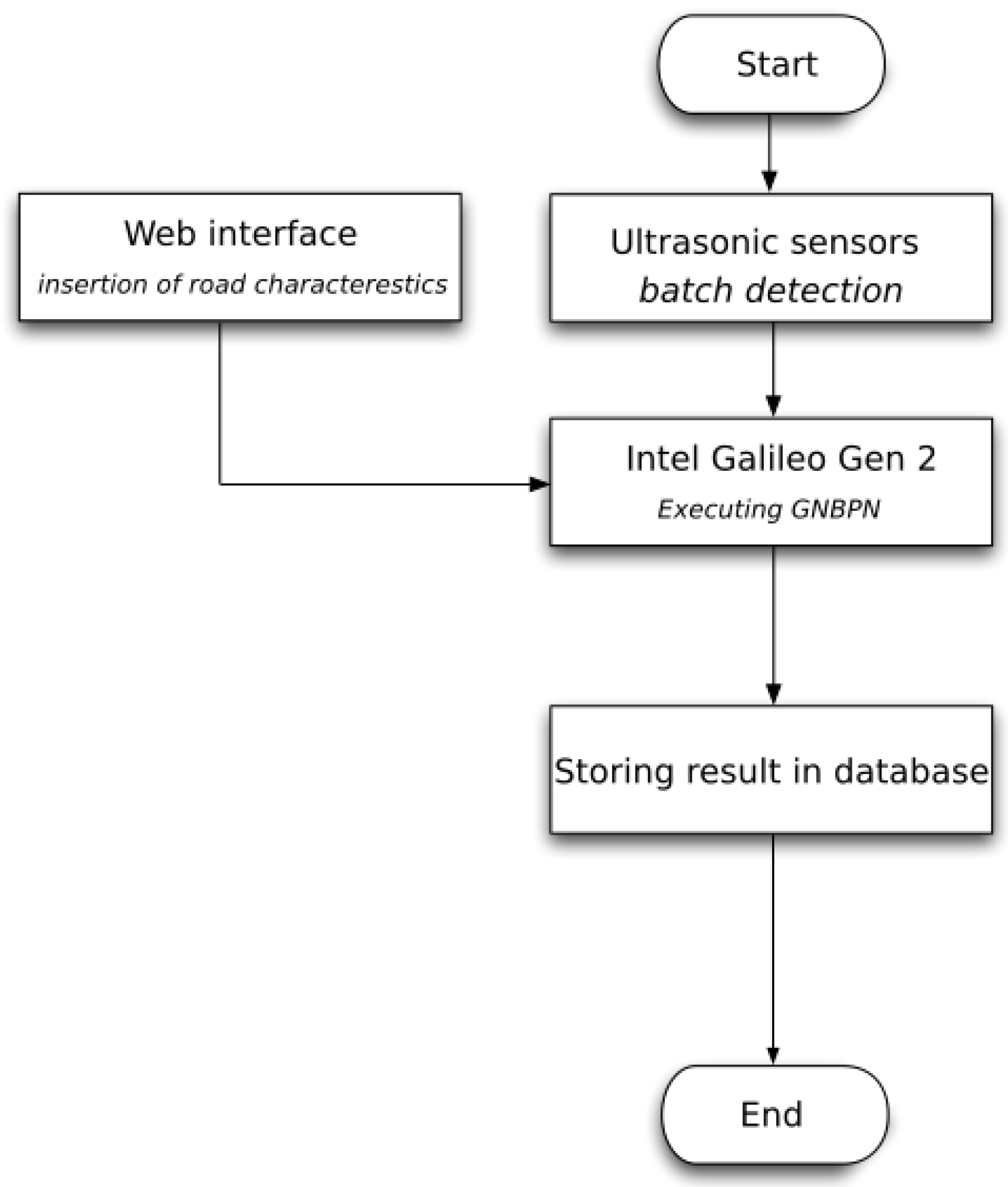
Figure 9 represents a workflow diagram for the developed prototype.
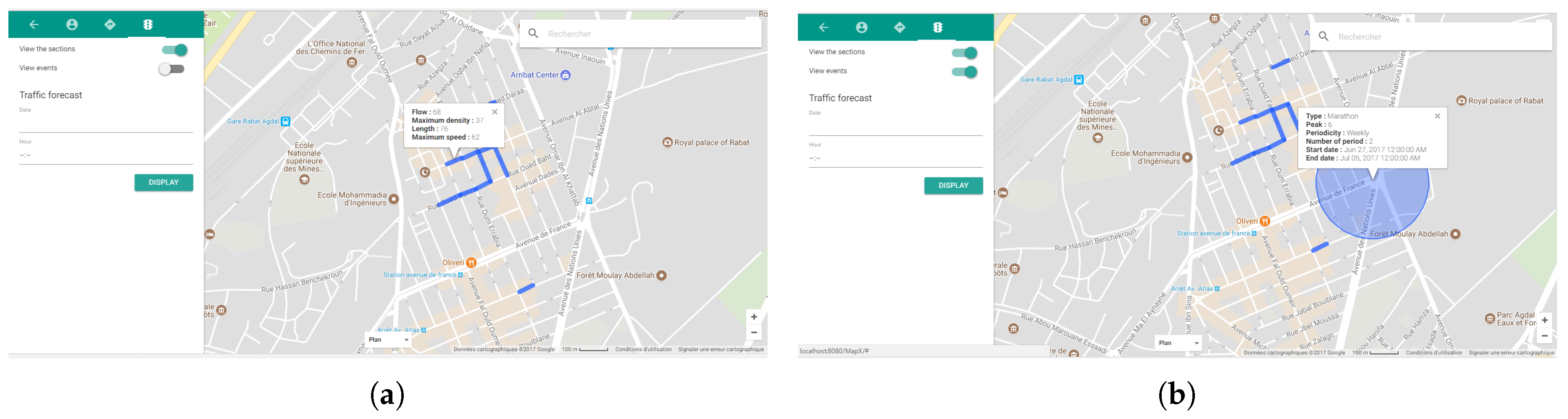
On another hand, based on our GNBPN model and estimation methods, we have developed color-coded visualizer that is used for viewing different segments of road network and estimating traffic evolution on (i) the same segments (temporal prediction) and (ii) related segments (spatial prediction). Different features are taken into consideration such as displaying traffic situations and computing travel times along possible routes for origin-destination pair etc. The visualizer takes the knowledge derived from models and turns it into easy and interpretable accessible visualizations that include near real-time road traffic flow, and road traffic prediction. Interaction with the system can be ensured through mobile applications or web portal (users) and dashboard (managers).
Figure 10 depicts a sample of the visualizer that we have developed. For instance, Figure 10a shows the level of congestion of a section that is characterized by flux, density, length and maximum speed. As for Figure 10b, it is an exploratory example of an event covers a circular geographical area, as well as the affluence that indicates its impact vis-à-vis the sections concerned.
We have used google map APIs for developing our color-coded visualizer described in the previous section and we have proceeded with customizing it by adding modules for CRUD operations on road segments using Java 8 and MySQL.
6. Conclusions
This paper presents a novel wireless sensor networks based system for road traffic management while detailing the deployment and the functional architectures.
The paper exhibits an implementation of two elements of the proposed system: Visualization and data analysis components. We are currently working on various components of the system :
- Implementation of the complete algorithm of our traffic state evolution
- Estimation of intersection turning movements and its implementation
- Using NoSQL database for data storage
Acknowledgments
The authors thank Joel Tankam, Bousseta Ayyoub and Ahmadou Youssef for their great help during the prototype development that contributed to improving the quality of our paper.
Author Contributions
This work is the result of the collective efforts of all authors. Youness Riouali conducted the research and trials. Laila Benhlima and Slimane Bah supervised the research and added their intellectual property and experience into the system. All the authors contributed to revision the paper and provided detailed comments to improve the content of the manuscript.
Conflicts of Interest
The authors declare no conflict of interest.
Abbreviations
The following abbreviations are used in this manuscript:
| WSN | Wireless Sensor Network |
| ITS | Intelligent Transportation System |
| ICT | Information and Communication technology |
| VANET | Vehicular Ad-hoc Network |
| HPN | Hybrid Petri nets |
| WTMS | WSN-based Traffic Management System |
References
- Losilla, F.; Garcia-Sanchez, A.J.; Garcia-Sanchez, F.; Garcia-Haro, J.; Haas, Z.J. A Comprehensive Approach to WSN-Based ITS Applications: A Survey. Sensors 2011, 11, 10220–10265. [Google Scholar] [CrossRef] [PubMed]
- Lazarescu, M.T. Design and Field Test of a WSN Platform Prototype for Long-Term Environmental Monitoring. Sensors 2015, 15, 9481–9518. [Google Scholar] [CrossRef] [PubMed]
- Darwish, A.; Hassanien, A.E. Wearable and Implantable Wireless Sensor Network Solutions for Healthcare Monitoring. Sensors 2011, 11, 5561–5595. [Google Scholar] [CrossRef] [PubMed] [Green Version]
- Conti, M. Secure Wireless Sensor Networks: Threats and Solutions; Advances in Information Security; Springer: New York, NY, USA, 2015. [Google Scholar]
- Mason, A.; Al-Shamma’a, A.I.; Shaw, A. Wireless Sensor Network for Intelligent Inventory Management for Packaged Gases. In Proceedings of the 2009 Second International Conference on Developments in eSystems Engineering, Abu Dhabi, UAE, 14–16 December 2009; pp. 413–417. [Google Scholar]
- Zhao, F.; Guibas, L. Wireless Sensor Networks: An Information Processing Approach; Electronics & Electrical; Morgan Kaufmann: Burlington, MA, USA, 2004. [Google Scholar]
- Liu, X.; Cao, J.; Lai, S.; Yang, C.; Wu, H.; Xu, Y.L. Energy efficient clustering for WSN-based structural health monitoring. In Proceedings of the 2011 IEEE INFOCOM, Shanghai, China, 10–15 April 2011; pp. 2768–2776. [Google Scholar]
- Giammarini, M.; Isidori, D.; Concettoni, E.; Cristalli, C.; Fioravanti, M.; Pieralisi, M. Design of Wireless Sensor Network for Real-Time Structural Health Monitoring. In Proceedings of the 2015 IEEE 18th International Symposium on Design and Diagnostics of Electronic Circuits Systems, Belgrade, Serbia, 22–24 April 2015; pp. 107–110. [Google Scholar]
- Bhattacharyya, S.; Deprettere, E.; Leupers, R.; Takala, J. Handbook of Signal Processing Systems; Springer: New York, NY, USA, 2013. [Google Scholar]
- Forster, C.A. Australian Cities: Continuity and Change; Meridian (Melbourne, Australia), Oxford University Press: Oxford, UK, 2004. [Google Scholar]
- Daven, J.; Klein, R. Progress in Waste Management Research; Nova Science Publishers: Hauppauge, NY, USA, 2008. [Google Scholar]
- Engelbrecht, J.; Booysen, M.J.; van Rooyen, G.J.; Bruwer, F.J. Survey of smartphone-based sensing in vehicles for intelligent transportation system applications. IET Intell. Transp. Syst. 2015, 9, 924–935. [Google Scholar] [CrossRef]
- Wang, Y.; Peng, Z.; Wang, K.; Song, X.; Yao, B.; Feng, T. Research on Urban Road Congestion Pricing Strategy Considering Carbon Dioxide Emissions. Sustainability 2015, 7, 10534–10553. [Google Scholar] [CrossRef]
- Alrawi, F. The importance of intelligent transport systems in the preservation of the environment and reduction of harmful gases. Transp. Res. Procedia 2017, 24, 197–203, 3rd Conference on Sustainable Urban Mobility, 3rd CSUM 2016, Volos, Greece, 26–27 May 2016. [Google Scholar] [CrossRef]
- Wang, R.; Xiao, F. Advances in Wireless Sensor Networks: 6th China Conference, CWSN 2012, Huangshan, China, October 25-27, 2012; Revised Selected Papers; Communications in Computer and Information Science; Springer: Berlin/Heidelberg, Germany, 2013. [Google Scholar]
- Bui, K.H.N.; Pham, X.H.; Jung, J.J.; Lee, O.J.; Hong, M.S. Context-Based Traffic Recommendation System. In Context-Aware Systems and Applications: Proceedings of the 4th International Conference, ICCASA 2015, Vung Tau, Vietnam, 26–27 November 2015; Vinh, P.C., Alagar, V., Eds.; Springer International Publishing: Cham, Switzerland, 2016; pp. 122–131. [Google Scholar]
- Ugnenko, E.; Uzhvieva, E.; Voronova, Y. Simulation of Traffic Flows on the Road Network of Urban Area. Procedia Eng. 2016, 134, 153–156, Transbaltica 2015: Proceedings of the 9th International Scientific Conference, Vilnius Gediminas Technical University, Vilnius, Lithuania, 7–8 May 2015. [Google Scholar] [CrossRef]
- Lv, Y.; Duan, Y.; Kang, W.; Li, Z.; Wang, F.Y. Traffic Flow Prediction With Big Data: A Deep Learning Approach. IEEE Trans. Intell. Transp. Syst. 2015, 16, 865–873. [Google Scholar] [CrossRef]
- Hoogendoorn, S.P.; Bovy, P.H.L. State-of-the-art of vehicular traffic flow modelling. Proc. I MECH E Part I J. Syst. Control Eng. 2001, 215, 283–303. [Google Scholar] [CrossRef]
- Arem, V.; Arem, B.V.; Hoogendoorn, S.P. Gas kinetic traffic flow modelling including continuous driver behaviour models. Transp. Res. Rec. J. Transp. Res. Board 2003, 1852, 1–19. [Google Scholar]
- Savrasovs, M. Traffic Flow Simulation on Discrete Rate Approach Base. Transp. Telecommun. J. 2012, 13, 167–173. [Google Scholar] [CrossRef]
- Treiber, M.; Kesting, A. Traffic Flow Dynamics; Springer-Verlag: Berlin/Heidelberg, Germany, 2013. [Google Scholar]
- Huang, B. GIS coupled with traffic simulation and optimization for incident response. Comput. Environ. Urban Syst. 2007, 31, 116–132. [Google Scholar] [CrossRef]
- Riouali, Y.; Benhlima, L.; Bah, S. Petri net extension for traffic road modelling. In Proceedings of the 2016 IEEE/ACS 13th International Conference of Computer Systems and Applications (AICCSA), Agadir, Morocco, 29 November–2 December 2016; Volume 7, pp. 7–12. [Google Scholar]
- Demongodin, I.; Audry, N.; Prunet, F. Batches Petri nets. In Proceedings of the IEEE Systems Man and Cybernetics Conference (SMC), Le Touquet, France, 17–20 October 1993; Volume 1, pp. 607–617. [Google Scholar]
- Demongodin, I. Generalised Batches Petri Net: Hybrid Model For High Speed Systems With Variable Delays. Discret. Event Dyn. Syst. 2001, 11, 137–162. [Google Scholar] [CrossRef]
- Riouali, Y.; Benhlima, L.; Bah, S. Toward a Global WSN-Based System to Manage Road Traffic. In Proceedings of the International Conference on Future Networks and Distributed Systems, Cambridge, UK, 19–20 July 2017; pp. 28:1–28:6. [Google Scholar]
- Xiao, L.; Peng, X.; Wang, Z.; Xu, B.; Hong, P. Research on Traffic Monitoring Network and Its Traffic Flow Forecast and Congestion Control Model Based on Wireless Sensor Networks. In Proceedings of the 2009 International Conference on Measuring Technology and Mechatronics Automation, Zhangjiajie, China, 11–12 April 2009; Volume 1, pp. 142–147. [Google Scholar]
- Rahman, M.; Ahmed, N.U.; Mouftah, H.T. City traffic management model using Wireless Sensor Networks. In Proceedings of the 2014 IEEE 27th Canadian Conference on Electrical and Computer Engineering (CCECE), Toronto, ON, Canada, 4–7 May 2014; pp. 1–6. [Google Scholar]
- Nafi, N.S.; Khan, R.H.; Khan, J.Y.; Gregory, M. A predictive road traffic management system based on vehicular ad-hoc network. In Proceedings of the 2014 Australasian Telecommunication Networks and Applications Conference (ATNAC), Southbank, Australia, 26–28 November 2014; pp. 135–140. [Google Scholar]
- Cárdenas-Benítez, N.; Aquino-Santos, R.; Magaña-Espinoza, P.; Aguilar-Velazco, J.; Edwards-Block, A.; Medina Cass, A. Traffic Congestion Detection System through Connected Vehicles and Big Data. Sensors 2016, 16, 599. [Google Scholar]
- Iwasaki, Y.; Misumi, M.; Nakamiya, T. Robust Vehicle Detection under Various Environmental Conditions Using an Infrared Thermal Camera and Its Application to Road Traffic Flow Monitoring. Sensors 2013, 13, 7756–7773. [Google Scholar] [CrossRef] [PubMed]
- Viola, P.; Jones, M. Rapid object detection using a boosted cascade of simple features. In Proceedings of the 2001 IEEE Computer Society Conference on Computer Vision and Pattern Recognition, (CVPR), Kauai, HI, USA, 8–14 December 2001; Volume 1, pp. I-511–I-518. [Google Scholar]
- Lienhart, R.; Maydt, J. An extended set of Haar-like features for rapid object detection. In Proceedings of the International Conference on Image Processing, Rochester, NY, USA, 22–25 September 2002; Volume 1, pp. I–900–I–903. [Google Scholar]
- Du, R.; Chen, C.; Yang, B.; Lu, N.; Guan, X.; Shen, X. Effective Urban Traffic Monitoring by Vehicular Sensor Networks. IEEE Trans. Veh. Technol. 2015, 64, 273–286. [Google Scholar] [CrossRef]
- Singh, V.; Srivastava, H.; Venturino, E.; Resch, M.; Gupta, V. Modern Mathematical Methods and High Performance Computing in Science and Technology: M3HPCST, Ghaziabad, India, December 2015; Springer: Singapore, 2016. [Google Scholar]
- Mikolajczak, B.; Singh, A. TransCPN—Software Tool for Transformation of Colored Petri Nets. In Proceedings of the 2009 Sixth International Conference on Information Technology: New Generations, Las Vegas, NV, USA, 27–29 April 2009; pp. 211–216. [Google Scholar]
- Martínez, D.; González, A.; Blanes, F.; Aquino, R.; Simo, J.; Crespo, A. Formal Specification and Design Techniques for Wireless Sensor and Actuator Networks. Sensors 2011, 11, 1059–1077. [Google Scholar] [CrossRef] [PubMed]
- Ehrig, H.; Juhas, G.; Padberg, J.; Rozenberg, G. Unifying Petri Nets: Advances in Petri Nets; Lecture Notes in Computer Science; Springer: Berlin/Heidelberg, Germany, 2003. [Google Scholar]
Figure 1.
Traffic management system (WTMS) architecture.

Figure 2.
Signalized road and the HPN model.

Figure 3.
T-intersection with give way rule, as depicted in the example.

Figure 4.
Generalized nondeterministic batch Petri net representation of traffic flow of the use case.
Figure 4.
Generalized nondeterministic batch Petri net representation of traffic flow of the use case.
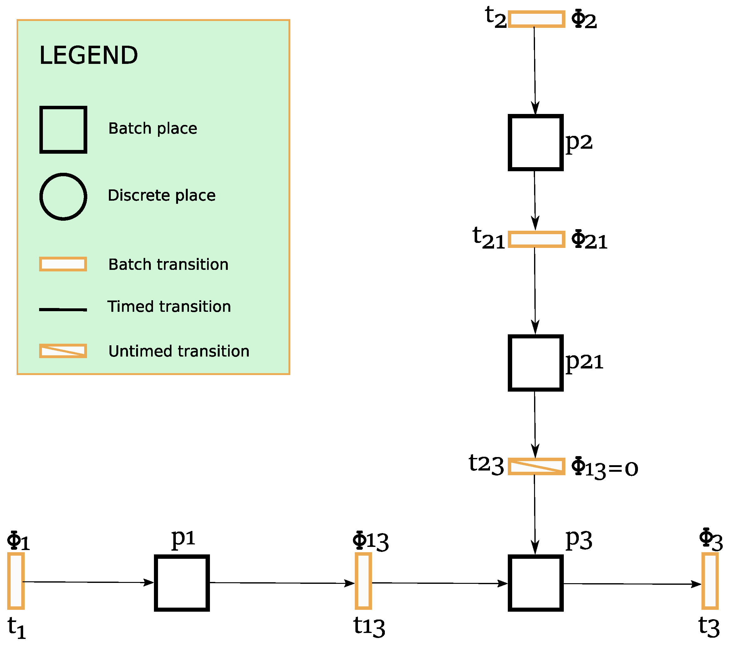
Figure 5.
Major components of the proposed architecture.
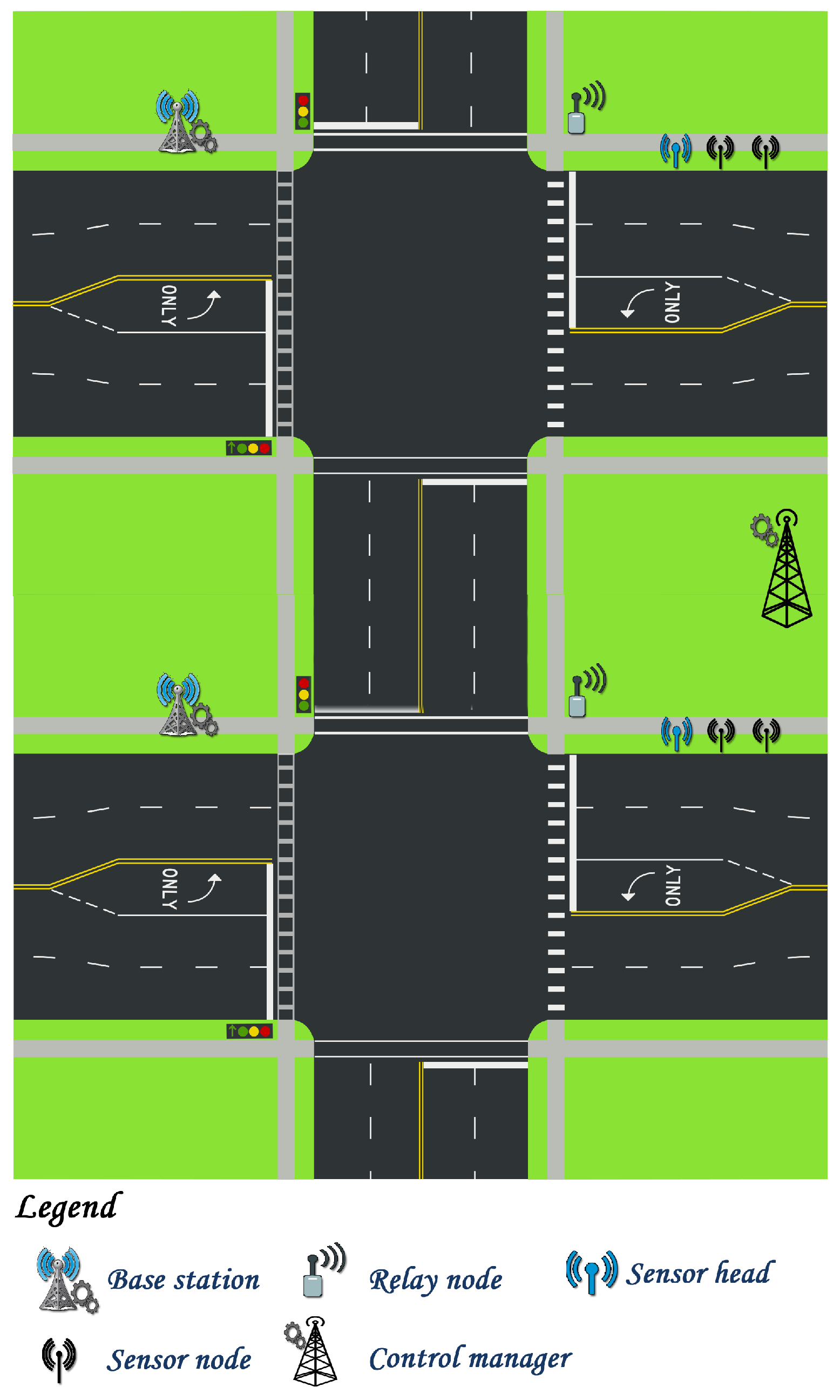
Figure 6.
A simple scenario of the proposed traffic management.

Figure 7.
screen of the Arduino IDE program with a sample sketches loaded of GNBPN model.

Figure 8.
The main elements of the proposed prototype. (a) HC-SR04 ultrasonic sensors with Intel Galileo Gen 2; (b) Web Interface for inserting road parameters.
Figure 8.
The main elements of the proposed prototype. (a) HC-SR04 ultrasonic sensors with Intel Galileo Gen 2; (b) Web Interface for inserting road parameters.
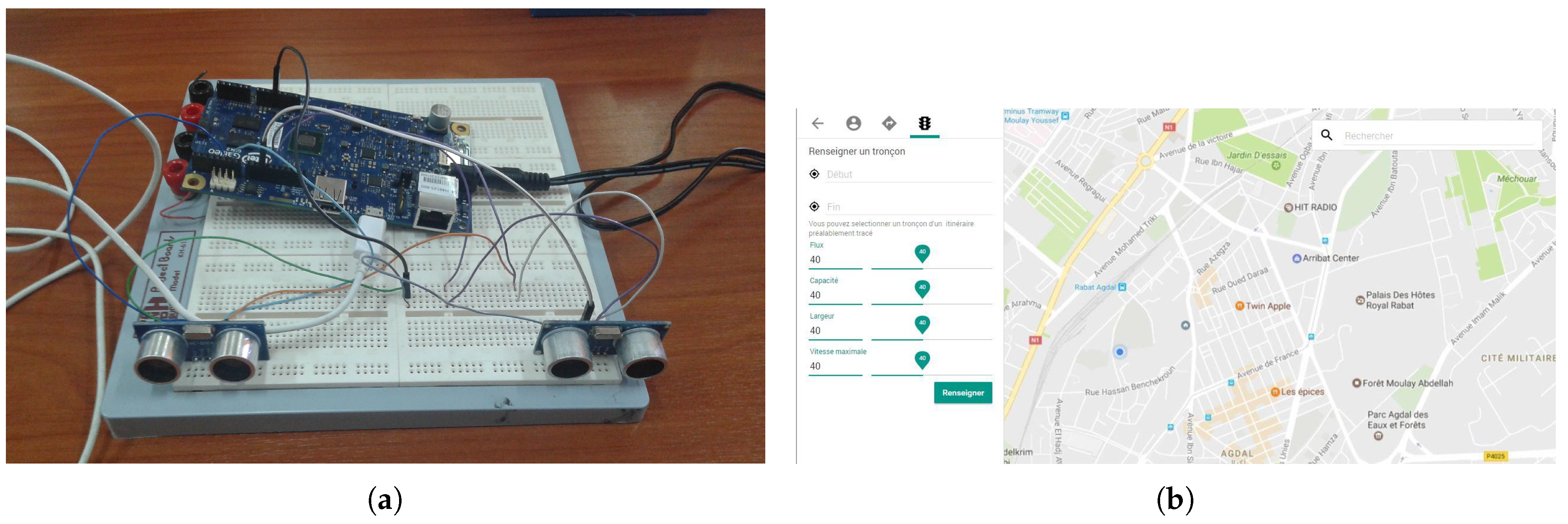
Figure 9.
The flow diagram of the developed prototype.

Figure 10.
Illustration of the road network visualizer application. (a) The main characteristics of a road section; (b) An event occurs in a geographical area.
Figure 10.
Illustration of the road network visualizer application. (a) The main characteristics of a road section; (b) An event occurs in a geographical area.

© 2017 by the authors. Licensee MDPI, Basel, Switzerland. This article is an open access article distributed under the terms and conditions of the Creative Commons Attribution (CC BY) license (http://creativecommons.org/licenses/by/4.0/).
Share and Cite
MDPI and ACS Style
Riouali, Y.; Benhlima, L.; Bah, S. Extended Batches Petri Nets Based System for Road Traffic Management in WSNs. J. Sens. Actuator Netw. 2017, 6, 30. https://doi.org/10.3390/jsan6040030
AMA Style
Riouali Y, Benhlima L, Bah S. Extended Batches Petri Nets Based System for Road Traffic Management in WSNs. Journal of Sensor and Actuator Networks. 2017; 6(4):30. https://doi.org/10.3390/jsan6040030
Chicago/Turabian StyleRiouali, Youness, Laila Benhlima, and Slimane Bah. 2017. "Extended Batches Petri Nets Based System for Road Traffic Management in WSNs" Journal of Sensor and Actuator Networks 6, no. 4: 30. https://doi.org/10.3390/jsan6040030
Note that from the first issue of 2016, this journal uses article numbers instead of page numbers. See further details here.