Using Sensors to Study Home Activities †


1
Centre for Research in Social Simulation, University of Surrey, Guildford GU2 7XH, UK
2
5G Innovation Centre, University of Surrey, Guildford GU2 7XH, UK
*
Author to whom correspondence should be addressed.
†
This paper is an extended version of Jiang, J.; Pozza, R.; Gunnarsdóttir, K.; Gilbert, N.; Moessner, K. Recognising Activities at Home: Digital and Human Sensors. In Proceedings of the International Conference on Future Networks and Distributed Systems, Cambridge, UK, 19–20 July 2017; ACM: New York, NY, USA, 2017; ICFNDS’17, pp. 17:1–17:11.
J. Sens. Actuator Netw. 2017, 6(4), 32; https://doi.org/10.3390/jsan6040032
Submission received: 1 November 2017
/
Revised: 3 December 2017
/
Accepted: 13 December 2017
/
Published: 16 December 2017
(This article belongs to the Special Issue Sensors and Actuators in Smart Cities)
Abstract
:Understanding home activities is important in social research to study aspects of home life, e.g., energy-related practices and assisted living arrangements. Common approaches to identifying which activities are being carried out in the home rely on self-reporting, either retrospectively (e.g., interviews, questionnaires, and surveys) or at the time of the activity (e.g., time use diaries). The use of digital sensors may provide an alternative means of observing activities in the home. For example, temperature, humidity and light sensors can report on the physical environment where activities occur, while energy monitors can report information on the electrical devices that are used to assist the activities. One may then be able to infer from the sensor data which activities are taking place. However, it is first necessary to calibrate the sensor data by matching it to activities identified from self-reports. The calibration involves identifying the features in the sensor data that correlate best with the self-reported activities. This in turn requires a good measure of the agreement between the activities detected from sensor-generated data and those recorded in self-reported data. To illustrate how this can be done, we conducted a trial in three single-occupancy households from which we collected data from a suite of sensors and from time use diaries completed by the occupants. For sensor-based activity recognition, we demonstrate the application of Hidden Markov Models with features extracted from mean-shift clustering and change points analysis. A correlation-based feature selection is also applied to reduce the computational cost. A method based on Levenshtein distance for measuring the agreement between the activities detected in the sensor data and that reported by the participants is demonstrated. We then discuss how the features derived from sensor data can be used in activity recognition and how they relate to activities recorded in time use diaries.
1. Introduction
Social researchers take a great interest in household practices, among other things, family dynamics and child-rearing (e.g., [1,2]), practices around meals [3], sleep [4], assisted living arrangements and mobile health solutions (e.g., [5,6]), homeworking [7] and energy-related practices [8]. Existing social research methods are both qualitative and quantitative, and often some combination of the two are used for pragmatic and constructivist purposes [9].
Qualitative methods are used to acquire rich in-depth data. Observations and open-ended interviews are particularly effective in capturing the meanings participants attach to various aspects of their everyday lives and relations (e.g., [10]). Quantitative methods such as questionnaires and surveys capture qualitative information in formalised ways for computational processing, and are widely used in large scale studies on demographics, household economics and social attitudes (e.g., [11,12]). Time-use diaries are also used to log activity sequences [13], and to seek evidence of life changes and social evolution [14]. Efforts to harmonise time use surveys across Europe have delivered guidelines (HETUS) [15] on activity coding for analysing the time use data, but interviews and observations are commonly used to cross-validate what goes on, and to calibrate and amplify the meaning of the diary evidence, including the use of activity sensors and video cameras [16].
Sensor-generated data are becoming widely available and the topic of activity recognition [17] has thrived in recent years with applications in areas such as smart homes and assisted living. Researchers have investigated activity recognition methods using data obtained from various types of sensors, for instance, video cameras [18], wearables [19] and sensors embedded in smartphones [20]. Such rich contextual information has been used in various activity specific studies. For example, Williams et al. [4] discuss the use of accelerometers to study people’s sleep patterns. Amft and Tröster [21] study people’s dietary behaviour by using inertial sensors to recognise movements, a sensor collar for recognising swallowing and an ear microphone for recognising chewing. Wang et al. [22] help in detecting elderly accidental falls by employing accelerometers and cardiotachometers.
Numerous algorithms have been proposed for general activity recognition in the literature, most of which are based on the assumption that by sensing the environment it is possible to infer which activities people are performing. Dynamic Bayesian Networks (e.g., [23]), Hidden Markov Models (e.g., [24]) and Conditional Random Fields (e.g., [25]) are popular methods due to their ability to recognise latent random variables in observing sequences of sensor-generated data. Other approaches rely on Artificial Neural Networks (e.g., [26]). A more detailed discussion will be given in Section 2.
To evaluate the adequacy of inferences about activities derived from sensor data, records of what activities are taking place from direct observation can be used to obtain the so-called “ground truth”. In the literature, there are three main types of approaches. The first relies on video cameras to record what participants are doing during an experiment. For example, Lin and Fu [23], use multiple cameras and floor sensors to track their participants. Although the data quality can be guaranteed in a controlled lab, this method is very intrusive and difficult to deploy in an actual home. A second common way of establishing ground truth is by asking participants to carry out a predefined list of tasks, again, in a controlled environment. For example, Cook et al. [27] ask their participants to carry out scripted activities, predetermined and repeatedly performed. Both of these methods correspond with social research methods, such as questionnaires, surveys and interviews, in generating what Silverman calls “researcher-provoked” data [28]. The outcomes may suffer the bias introduced by the researchers in provoking participants’ activities as opposed to observing them without interference. The third type of approach relies on human annotators to label sensor-generated data manually. For example, Wang et al. [29] conducted a survey with their participants to have a self-reported record of their main activities, and compared it to the annotated data based on video recordings. This type of approach relies heavily on the annotator’s knowledge of participants’ activities and their understanding of participants’ everyday practices, but may also be challenged by discrepancies between the research-provoked survey and video data and non-provoked sensor-generated data.
In this study, we consider two data sources. The first is “digital sensors” that generate activity data based on activity recognition derived from sensor-generated environment data (referred to as sensor data or sensor-generated data in the rest of the paper). The second is “human sensors” that generate activity data from participants’ self-reported time-use diaries (referred to as time use diary or self-reported data in the rest of the paper). To make inferences from sensor data about human activities, it is first necessary to calibrate the sensor data by matching the data to activities identified by the self-reported data. The calibration involves identifying the features in the sensor data that correlate best with the self-reported activities. This in turn requires a good measure of the agreement between the activities detected from sensor-generated data and those recorded in self-reported data.
To illustrate how this can be done, we conducted a trial in three residential houses, collecting data from a set of sensors and from a time use diary recorded by the occupant (human sensor) from each house over four consecutive days. The sensors captured temperature, humidity, range (detecting movements in the house), noise (decibel levels), ambient light intensity (brightness) and energy consumption. For activity recognition, we adopt an unsupervised learning approach based on a Hidden Markov Model, i.e., only sensor-generated data are used to fit the model, which allows the model to discover the patterns by itself rather than fitting the model with unreliable labels from the time use diaries. We apply mean shift clustering [30] and change points detection [31] for extracting features. To reduce computational cost, we adopt a correlation-based approach [32] for feature selection. To compare the data generated by the two types of sensors, we propose a method for measuring the agreement between them based on the Levenshtein distance [33].
The contributions of this paper are three-fold. First, we present a new data collection framework for recognising activities at home, i.e., a mixed-methods approach of combining computational and qualitative types of non-provoked data: sensor-generated and time use diary. Secondly, we investigate the application of several feature extraction and feature selection methods for activity recognition using sensor-generated data. Thirdly, we propose an evaluation method for measuring the agreement between the sensor-supported activity recognition algorithms and the human constructed diary. Compared to our previous work [34], this paper has the following extensions: (1) we add an illustration of the trial setup procedure and discuss the design of the procedure; (2) we use a larger data set of three households and investigate three more activity types; (3) we demonstrate the use of feature selection in activity recognition to harness the exploration of feature combinations; and (4) we further the analysis of results by triangulating with evidence from household interviews.
The rest of the paper is organised as follows. In Section 2, we discuss related work. In Section 3, we give an introduction to the home settings. Thereafter, in Section 4, we describe the data collected for this study, including both the sensor data and the time use diary data. In Section 5, we show how features are extracted and selected and introduce our activity recognition algorithm. In Section 6, we present the metric for evaluating agreement between activities recognised by the sensor-generated data and what is reported by the participant, and give an analysis of the results based on the evidence gathered from household interviews. Finally, we conclude our work with some possible extensions in Section 7.
2. Related Work
In this section, we discuss the works that have been recently published in the area of automated activity recognition in home-like environments in terms of the sensors they use, the activities they detect, and the recognition methods they adopt or propose.
Early works (e.g., [23,35]) were concerned with designing frameworks for providing services based on the prediction of resident action. For example, Lin and Fu [23] leveraged K-means clustering and domain knowledge to create context out of raw sensor data and combined this with Dynamic Bayesian Networks (DBNs) to learn multi-user preferences in a smart home. Their testbed allows location tracking and activity recognition via cameras, floor sensors, motion detectors, temperature and light sensors in order to recommend services to multiple residents, such as turning on TV or lights in various locations or playing music.
More recently, the CASAS smart home project [36] enabled the detection of multi-resident activities and interactions in a testbed featuring motion, temperature, water and stove (ad-hoc) usage sensors, energy monitors, lighting controls and contact detectors for cooking pots, phone books and medicine containers. Using the testbed, Singla et al. [37] applied Hidden Markov Models (HMMs) to perform real-time recognition of activities of daily living. Their work explores seven types of individual activities: filling medication dispenser, hanging up clothes, reading magazine, sweeping floor, setting the table, watering plants, preparing dinner, and 4 types of cooperative activities: moving furniture, playing checkers, paying bills, gathering and packing picnic food. Validated against the same data set, Hsu et al. [25] employed Conditional Random Fields (CRFs) with strategies of iterative and decomposition inference. They found that data association of non-obstructive sensor data is important to improve the performance of activity recognition in a multi-resident environment. Chiang et al. [38] further improved the work in [25] with DBNs that extend coupled HMMs by adding vertices to model both individual and cooperative activities.
The single-occupancy datasets from CASAS also attracted many researchers. For example, Fatima et al. [39] adopted a Support Vector Machine (SVM) based kernel fusion approach for activity recognition and evaluated it on the Milan2009 and Aruba datasets. Fang et al. [40] evaluated the application of neural network for activity recognition based on a dataset of two volunteers. Khrishnan and Cook [41] evaluated an online sliding-window based approach for activity recognition on a dataset of three single-occupancy houses. The authors showed that combining mutual information based weighting of sensor events and adding past contextual information to the feature leads to better performance. To analyse possible changes in cognitive or physical health, Dawadi et al. [42] introduced the notion of activity curve and proposed a permutation-based change detection in activity routine algorithm. The authors validated their approach with a two-year smart home sensor data. In these works, different kinds of sensors were used such as temperature and light sensors, motion and water/stove usage sensors. The recognised activities range from common ones such as eating and sleeping to more specific ones like taking medication.
ARAS [43] is a smart home data set collected from two houses with multiple residents. The two houses were equipped with force sensitive resistors, pressure mats, contact sensors, proximity sensors, sonar distance sensors, photocells, temperature sensors, and infra-red receivers. Twenty-seven types of activities were labelled such as watching TV, studying, using internet/telephone/toilet, preparing/having meals, etc. With the ARAS dataset, Prossegger and Bouchachia [44] illustrated the effectiveness of an extension to the incremental decision tree algorithm ID5R, which induces decision trees with leaf/class nodes augmented by contextual information in the form of activity frequency.
With a mission of elderly care, the CARE project [45] has carried out research on automatic monitoring of human activities in domestic environments. For example, Kasteren et al. [46] investigated HMMs and CRFs for activity recognition in a home setting and proposed to use Bluetooth headsets for data annotation. Fourteen state-change sensors were placed on the doors, cupboards, refrigerator and toilet flush. Seven types of activities were annotated by the participants themselves, including sleeping, having breakfast, showering, eating dinner, drinking, toileting and leaving the house. Two probabilistic models, HMM and CRF, were investigated for activity recognition. Kasteren et al. [24] provided a summary of probabilistic models used in activity recognition and evaluated their performance on datasets of three households with single occupant. Further work by Ordonez et al. [47] evaluated transfer learning with HMMs on a dataset of three houses with the same setting of sensor deployment and labelled activity types, showing potential of reusing experience on new target houses where little annotated data is available.
Besides probabilistic models, neural network models are becoming popular in recognising human activities. For example, Fan et al. [26] studied three neural network structures (Gated Recurrent Unit, Long Short-Term Memory, Recurrent Neural Network) and showed that a simple structure that remembers history as meta-layers outperformed recurrent networks. The sensors they used include grid-eye infrared array, force and noise sensors as well as electrical current detectors. For their model training, the participants performed scripted activities in a home testbed: eating, watching TV, reading books, sleeping and friends visiting. Singh et al. [48] showed that Long Short-Term Memory classifiers outperformed probabilistic models such as HMM and CRF when raw sensor data was used. Laput et al. [49] proposed a general-purpose sensing approach with a single sensor board that is capable of detecting temperature, humidity, light intensity and colour, motion, sound, air pressure, WiFi RSSI, magnetism (magnetometer) and electromagnetic inference (EMI sensor). The sensors were deployed in five different locations including a kitchen, an office, a workshop, a common area and a classroom. For activity recognition, a supervised approach based on SVM and a two-stage clustering approach with AutoEncoder were used. The authors showed the merit of the sensor features with respect to their contribution to the recognition of 38 types of activities.
While several other approaches exist for activity recognition and capture, they mostly employ only wearable sensors (i.e., see [19] for a recent survey), and thus cannot be applied in multi-modal scenarios of smart-home settings with fixed, unobtrusive and ambient sensors. In addition, due to the time-series nature of activity recognition in the home environment, supervised algorithms not incorporating the notion of temporal dependence might lead to poor performance in activity recognition, so such works are not reviewed here.
Time use diaries are widely used for collecting activity data. To validate time use diaries, Kelly et al. [16] tested the feasibility of using wearable cameras. Participants were asked to wear a camera and at the same time keep a record of time use over a 24-hour period. During an interview with each participant afterwards, the visual images were used as prompts to reconstruct the activity sequences and improve upon the activity record. No significant differences were found between the diary and camera data with respect to the aggregate totals of daily time use. However, for discrete activities, the diaries recorded a mean of 19.2 activities per day, while the image-prompted interviews revealed 41.1 activities per day. This raises concerns of using the data collected from time use diaries for training activity recognition models directly.
In this work, we use a suite of fixed sensors. For activity recognition, we build our model based on HMMs. In particular, we investigate the use of mean shift clustering and change points detection techniques for feature extraction. A correlation-based feature selection method is applied to reduce computational cost. Our work differs from similar studies in that we adopt a mixed-methods approach for the problem of recognising activities at home, and we evaluate its effectiveness using a formal framework.
3. Experiment Setting
For this work, we installed a suite of sensors in three households. The data collected by the sensors were encrypted and sent to a central server over the Internet.
3.1. Sensor Modules
We used six types of sensor modules, as summarised in Table 1.
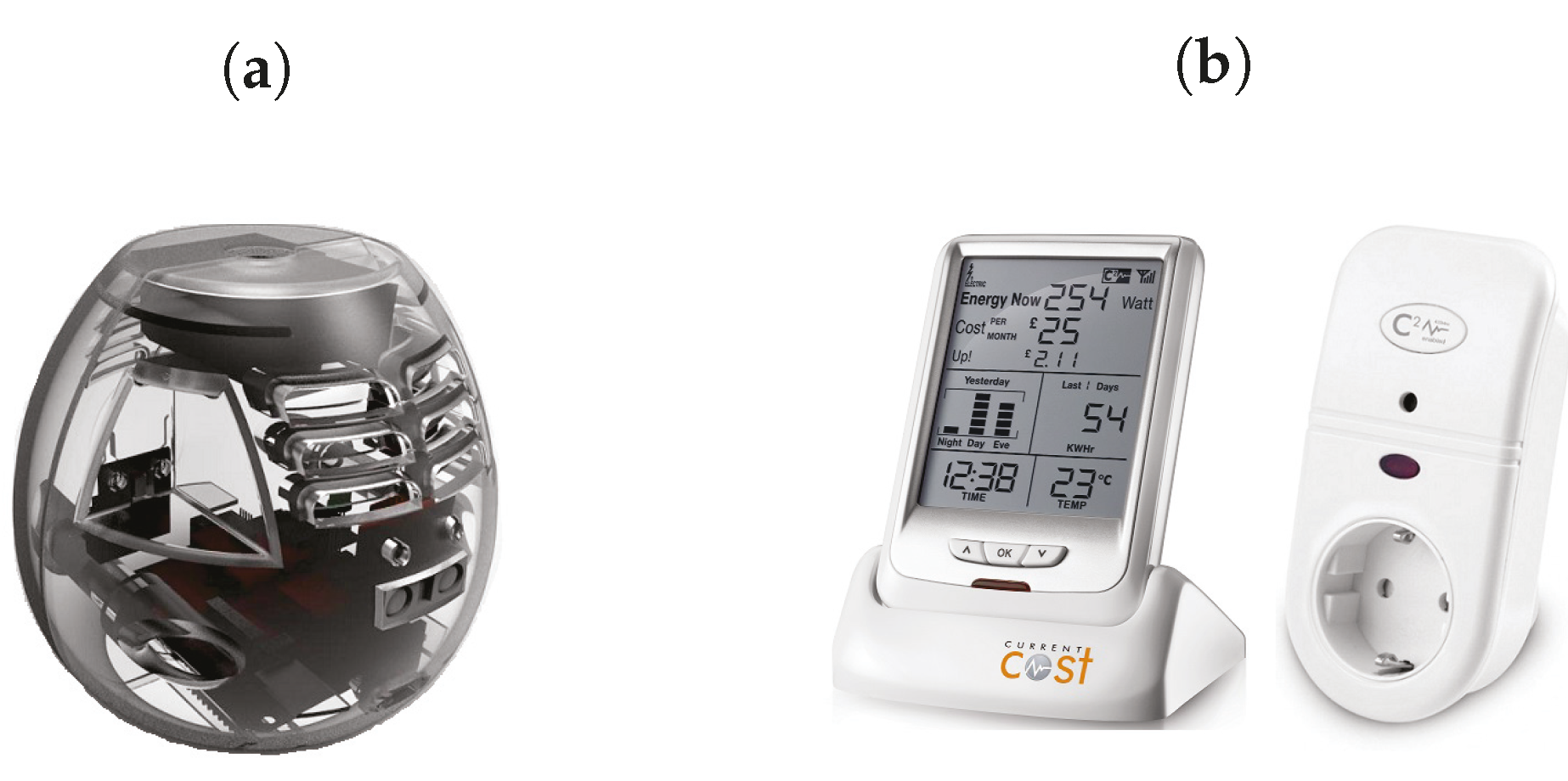
The first five sensor modules are encapsulated in a sensor box, as shown in Figure 1a, coordinated by a Seeeduino Arch-Pro [50]. The temperature and humidity sensor HTU21D [51] is managed via an I2C interface and sampled periodically by the client application deployed on the ARM core. An Avago ADPS-9960 light sensor [52] , also managed via an I2C interface, is used to sample ambient light measured in . The GP2Y0A60SZ ranging sensor from Sharp [53] is an analog sensor with a wide detection range of 10 cm to 150 cm, which is sampled via a 12 bit ADC and converted through the manufacturer’s calibration table. Finally, the MEMS Microphone breakout board INMP401 [54] is used to sample noise levels in the environment via an ADC and the values are converted to decibels (dB SPL).
The other sensor module used in this work is a commercial electricity monitoring kit from CurrentCost [55], as shown in Figure 1b. It features a current transformer (CT) clamp, a number of individual appliance monitors (IAMs) and a transmitter to measure the energy consumption in watts of the whole house as well as the individual appliances.
Compared to the works discussed in Section 2, the sensor modules used for this work require little effort on part of the participants.
3.2. Demonstration and Installation
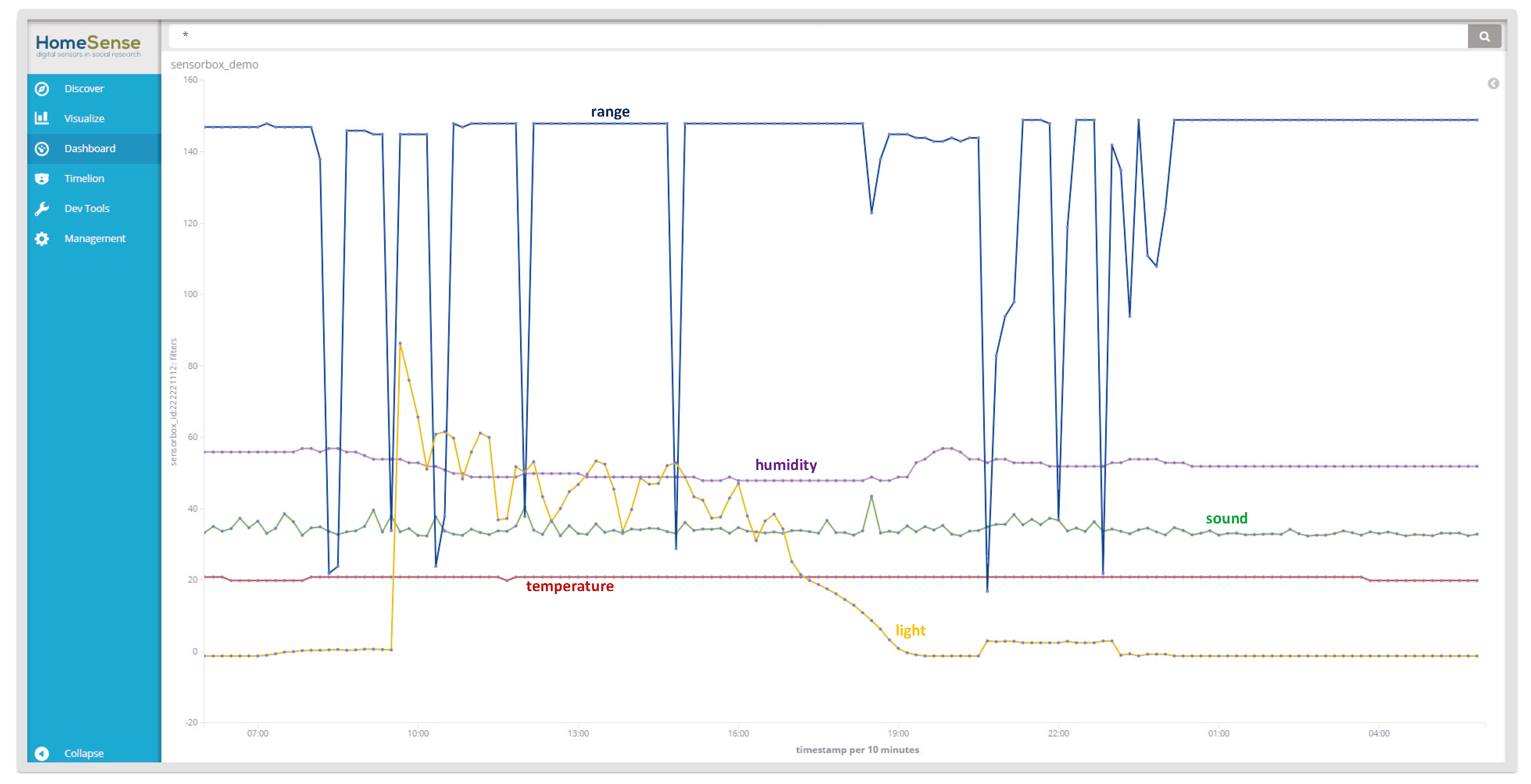
For each household, we first set up an interview with the participants, in which we demonstrate the workings of the sensor platform to demystify the experiment, e.g., to show what kinds of data are collected, and what can be seen in the data. Figure 2 shows the interface of our sensor data collection and visualisation platform. Participants can interact with the sensors, e.g., turn electrical equipment on and off, move in front or make loud noise around a sensor box, breathe on it, etc., and see in real time the changes of corresponding sensor readings.
Thereafter, we ask the participants to give a tour of their house and explain what goes on at different times in different rooms, who is involved, and so on. However, they are free to omit any room or area of the house. A sketch of the floor plan with markings of potential places for installing sensors is produced in the meantime.
After the interview, another appointment is made for sensor installation. During the installation, the participants guide the researchers around the house and negotiate the location for placing the sensors.
3.3. Trial Households
Three trial households are included in the experiment presented here, each with a single occupant. Table 2 shows the house composition and the sensor deployment.
For all the three houses, there was at least one sensor installed in each room, except bathrooms which do not have electrical outlets in the UK. The number of sensor boxes installed in each room depends on the size of the room. The locations where the sensor boxes were installed were meant to cover as much as possible of the room space but were sometimes constrained by the availability of power supply. A selection of more commonly used home appliances were attached to individual energy monitors. Their energy consumption as well as the total consumption for each of the households were also recorded.
4. Data Sets
In the experiment, two types of data were collected, sensor-generated data and time use diaries. The time use diaries cover a period of four consecutive days for all three households between June and July 2017 from 6:00 a.m. on the first day until 5:50 a.m. on the last day. The sensor-generated data set covers an extended period from 6:00 p.m. on the previous day of the starting date (time use diary) and to 12:00 p.m. of the last day (time use diary). The reason for such an extension is to incorporate the relevant signals before and after the recorded time use which will be illustrated in Section 5.1.
4.1. Sensor-Generated Data
The sensor-generated data consists of readings from the six types of sensor modules as shown in Table 1.
The data from sensor boxes were collected around every three seconds. An example reading from a sensor box is shown as follows:
{“Box_ID”: 123, “Timestamp”: 2016-12-13 09:00:00, “Temperature”: 20,
“Humidity”: 50, “Sound”: 45, “Range”: 100, “Light”: 583}
“Humidity”: 50, “Sound”: 45, “Range”: 100, “Light”: 583}
For , the lowest values among samples at 1000 Hz within each period of three seconds was collected, i.e., the distance to the nearest object that has been detected in the period of three seconds. This is to minimise the number of false negative detections which may happen when only collecting samples at a point of time every three seconds. Noise level (sound) is derived from an on-device conversion of air pressure changes (sampling at around 1000 Hz) to decibels (dB). The readings from all the other sensor modules are sampled once every three seconds.
The data from electricity monitors (IAMs) was collected around every six seconds. An example reading from an IAM is shown as follows:
{“IAM_ID”: 123, “Timestamp”: 2016-12-13 09:00:00, “Watts”: 100}
The sensor boxes can capture various environmental changes but not all the changes are caused by human activities. For example, the weather can be an important factor influencing temperature and humidity. By carefully modelling the changes, we may be able to distinguish those caused by human activities from those caused by external factors as they differ in terms of magnitude and frequency.
Table 3 shows the statistics about the total number of readings of the sensor-generated data used in this work with respect to the three households.
The multiplier 5 in the second column indicates that each reading from a sensor box consists of five data attributes corresponding to the five sensor modules as shown in Table 1.
4.2. Time Use Diary
During the four days of the experiment, the occupant from each household was asked to keep a diary of time use based on the HETUS model [15]. The participants were asked to update the diary at 10-minute intervals except sleeping and keep track of the 10 minutes interval using their own preferred method, e.g. setting up a timer. The diary was paper-based and the participants were given instructions on how to fill the diary using pens and shorthand. For example, an arrow can be used to mark an activity that takes longer than 10 minutes. However, given the heavy workload of filling such a diary, it is very likely that the participants may not have strictly followed the guidelines, as will be further illustrated in Section 6.1.
Table 4 gives a partial sample of what is recorded: the participant specifies for every 10 minutes what he or she has been doing primarily (and possibly secondarily) in which location/room (possibly with the assistance of or involving devices). For each household, there is at least one activity recorded by the occupant at each of the 10 minutes slots over the course of four days, which produces in total 576 data points from the diary.
In this study, we focus on seven types of home activities that have been recorded in the time use diaries: sleeping, preparing meal, making hot drink (tea or coffee), eating (breakfast, lunch or dinner), watching TV, listening to radio, and doing laundry. It has to be noted that these are not the only activities the participants reported in their diaries. These seven activity types are selected because they were reported by the occupants from all the three households and occur at a relatively higher frequency or last for a relatively longer time. Table 5 shows a summary of how many times each type of activity occurred and their duration in each household.
Household 1 does not have a radio while the occupant had the TV turned on a lot of the time. Household 3 does not have a TV while the occupant had the radio turned on a lot of the time. Notice that for each household the total percentage of time designated to the seven activity types does not sum up to 100% because other activities carried out by the occupants are not listed in the table.
4.3. Data Reliability
In this section, we analyse the reliability of sensor-generated data in parallel form via the Pearson correlations between readings from each pair of sensors that are of the same type and placed in the same room (see Table 2). Table 6 summaries the correlations.
It can be seen that sensor readings from the same type of sensor in the same room have a strong correlation except for the readings from all pairs of ranging sensors and the pair of temperature sensors in Household 2 (living/dining room). The relatively low correlations between ranging sensors may relate to the fact that: (1) ranging sensors have a limited sensing capability (up to 150 cm); and (2) one of our guidelines of installing sensors is to cover as much room space as possible, i.e., ranging sensors (sensor boxes) are placed to capture movements in different parts of the room. Therefore, it is expected that only one of the ranging sensors is triggered at any given time. As for the pair of temperature sensors, the relatively low correlation may be due to their positions in the room, i.e., one of the sensor boxes is placed near the window and the other is placed away from the window.
In Section 6, we will further discuss inter-rater/observer reliability by means of the agreement between sensor-generated data and human recorded time use diary.
5. Recognising Activities
Sensor-generated data provides a digital means of looking into the life of a household. Such data in itself does not tell directly what is taking place but it provides rich contextual information drawn from the aggregate of environmental variables. Our objective in this section is to investigate what kinds of features can be drawn from the sensor-generated data and how such features can be used for activity recognition.
5.1. Feature Extraction
Activities give rise to changes in sensor readings. For example, when cooking, the temperature may rise in the kitchen because of the heat emitted from the hob, humidity levels go up and range readings may fluctuate intensively because of the physical movements involved. These types of changes in the sensor-generated data are essential to better understand the context of activities and to recognise their occurrence.
There are two types of patterns in the sensor readings observed in our experiments. The first type is clusters, i.e., absolute values of sensor readings appear naturally in clusters. For example, the readings of the ranging sensor are either the maximum value during periods when nothing comes in and out of range or distinctly much smaller values. The second type relates to the distribution changes of sensor readings along the time dimension, thus taking into account both time dependency and value changes between sensor readings.
Accordingly, we investigate the application of three methods for extracting features from sensor-generated data. The first, mean shift [30], aims at clustering the readings of sensor data into different value bands. The second method, change points detection [31], aims at finding meaningful points of change in the sequences of sensor-generated data. The third method, change points gap detection, which is based on the second method, aims at identifying the length of stable periods of readings in sensor-generated data. In our experiment setting, we apply these three feature extraction methods upon the re-sampled data, which is detailed in the next section.
5.1.1. Re-Sampling
To align with the time use diary and synchronise the data from the different sensors (sensor box and energy monitors), we re-sample the sensor data with bins of 10 minutes. Re-sampling is done using the maximum values for temperature, humidity, brightness, noise level, and the minimum values for range. To cover the time use diary and give buffers for feature extraction, we re-sample and use the sensor data from 6:00 p.m. on the day before the period of the time use diary to 12:00 p.m. on the day after that. The re-sampling results 685 data points (observations) for each sensor.
5.1.2. Mean Shift
Mean shift is a non-parametric clustering method that does not require prior knowledge of the number of clusters. It is based on an iterative procedure that shifts each data point to its nearest local mode, by updating candidates for centroids to be the mean of the data points within its neighbourhood [30].
Given a set of data points S in a n-dimensional Euclidean space X, mean shift considers these data points as sampled from some underlying probability density function and uses a kernel function for estimating the probability density function. In this work, we chose to use a flat kernel K with a bandwidth h, as defined below:
The sample mean at is
The difference is called mean shift and the mean shift algorithm is the procedure of repeatedly moving data points to the sample means until the means converge. In each iteration, s is updated by for all simultaneously. As a result, all the data points are associated with a centroid/cluster. Applying this procedure to the re-sampled raw sensor readings, each data point in the re-sampled dataset is represented by the index of its associated cluster. The implementation is based on python scikit-learn [56].
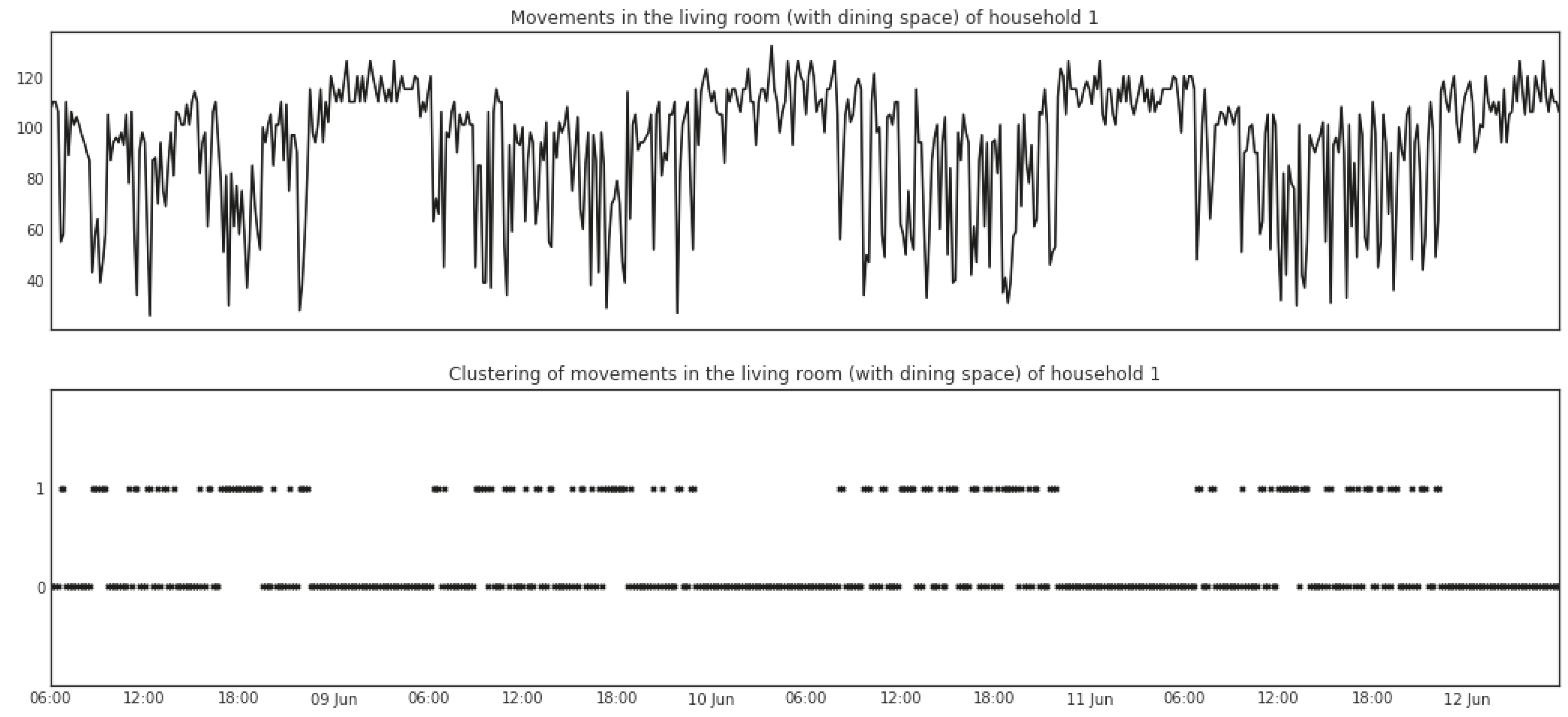
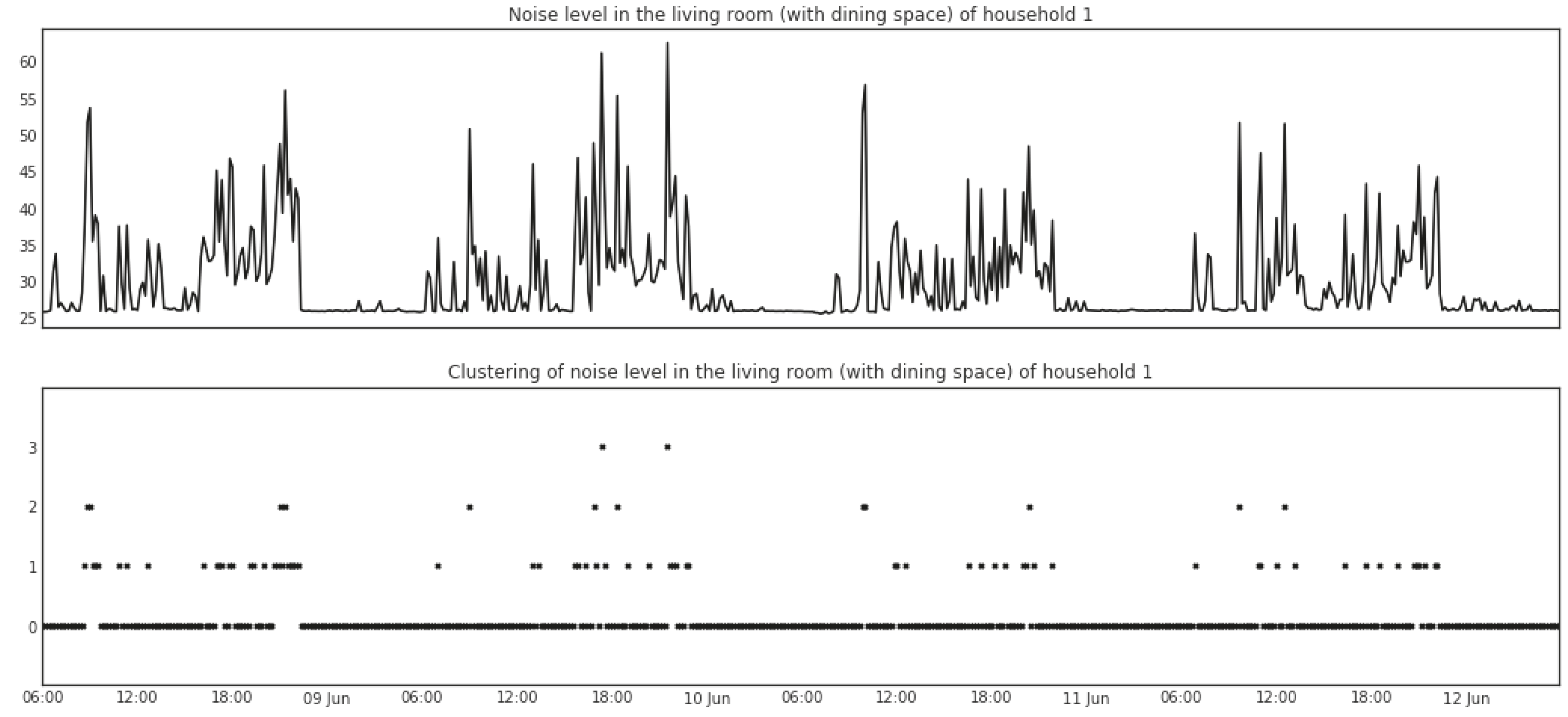
As an example, the lower parts of Figure 3 and Figure 4 show the results of features extracted via the mean shift clustering algorithm. The data depicted in the upper parts of the two figures are from range and noise-level readings in the living room (with dining space) of Household 1. The readings for range generate two clusters with indices of 0 and 1. A straightforward explanation is that the cluster with index 0 represents the times when no movements are detected in the room and the cluster with index 1 represents the times when movements are detected. As for the noise level, four clusters are generated with indices of 0, 1, 2, and 3, in which the cluster with index 0 represents the times when the kitchen is relatively quiet while the other three clusters represent increasingly higher levels of noise.
5.1.3. Change Points Detection
Change points detection is a method of estimating the times at which the statistical properties of a sequence of observations change [31].
Given a sequence of data, , a change is considered to occur when there exists a time such that the statistical properties of differ from that of , e.g., in mean or variance. In the case of multiple changes, a number of change points are identified, that split the sequence of data into segments.
The parameters of the change points distribution are estimated via maximum likelihood by minimising the following cost function:
where is a cost function for assuming a change point at in the time series data and is a penalty function to avoid over fitting (i.e., too many change points).
For our sensor data, we focus on detecting the changes of mean in the sensor readings. A manual setting is used for the penalty function so that the number of change points can be adjusted. The change points detection algorithm is the pruned exact linear time (PELT) [57] which is computationally efficient and provides an exact segmentation. By applying the change points detection algorithm upon the re-sampled data, we obtain a sequence of 1s and 0s, where “1” represents the presence of a change point and “0” as absence. The implementation is based on the R package introduced in [58].
5.1.4. Change Point Gaps
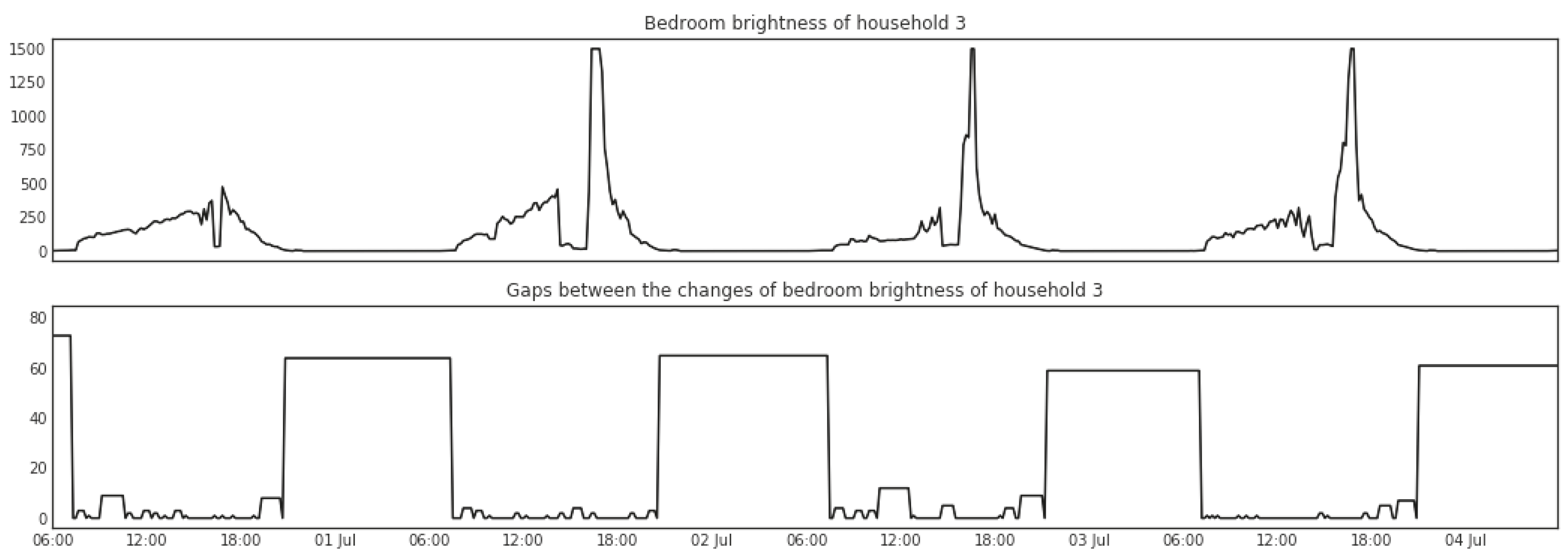
Change points detected in sensor signals indicate changes in the home environment, which may be caused by human activities. While the time periods during which no change of sensor signal is detected may on the other hand indicate the lasting of some activities. For instance, when the house is asleep we can expect a long gap between changes that are detected in electricity consumption and brightness in the house, i.e., from the time of going to bed to getting up, as shown in Figure 7 and Figure 8. Therefore, the length of gaps between change points can also be a useful feature to identify occurrences of activities. Given a sequence where represents the presence of a change point and represents the absence of a change point, the length of gaps between change points with respect to is calculated as follows:
where .
In the experiment, we apply the above gap detection to the change points inferred from each type of sensor reading.
Figure 7 shows big gaps between changes in the total energy consumption, indicated by the width and height of the bars, detected between midnight and early morning every night. A similar and aligned pattern can be found in the brightness of the bedroom as shown in Figure 8.
In this section, we presented three kinds of features (mean-shift clustering, change points, and gaps between change points) that can be extracted from the sensor-generated data, which expands the number of data values in each observation by three times. That is, for Household 1, there are 140 features extracted from the sensor readings of eight sensor boxes and six energy monitors; for Household 2, there are 123 features extracted from the sensor readings of seven sensor boxes and six energy monitors; and, for Household 3, there are 150 features extracted from the sensor readings of nine sensor boxes and five energy monitors. After feature extraction, we truncate the feature data points in the extended periods to match the time use diary. This reduces the number of feature data points from 685 to 576 for each type of sensor reading. The series of feature data points is at the frequency of one per 10 minutes.
5.2. Feature Selection
For different types of activities, some features are more relevant than the others. Given the size of the feature sets, it is intractable to evaluate all the possible subsets of the features. To this end, a feature selection process is necessary for finding a subset of features that can effectively describe the data while reducing irrelevant or highly-correlated inputs [59]. In this work, we adopt the approach proposed in [32], which is based on the heuristic that takes into account the usefulness of individual features for predicting the class labels along with their inter-correlations. A formalisation of the heuristic is given by [60]:
where represents the heuristic “merit” of a feature subset S containing k features, is the mean feature-class correlation (), and is the average feature-feature inter-correlation. The numerator indicates how predicative of the class a group of features is, while the denominator indicates how much redundancy there is within the group.
Following the proposal in [32], the metric of symmetrical uncertainty [61] is used for calculating feature-feature and feature-class correlations. Symmetrical uncertainty is based on the concept of information gain [62] while compensating for its bias towards attributes with more values and normalising its values to the range from 0 to 1.
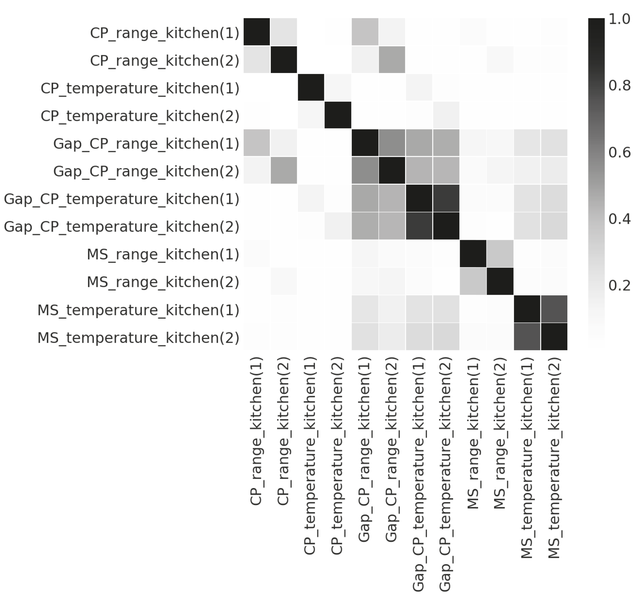
As an example, Figure 9 and Figure 10 show the feature-feature correlations between the sensor readings (temperature and range) of the two sensor boxes installed in the kitchen of Household 1, and the feature-class correlation between the sensor readings of electricity consumption and seven activity types in Household 3. The prefixes, , and , represent the feature extracted via the mean shift clustering, the change points detection, and the gaps between the detected change points. We can see in Figure 9 that the features extracted from the temperature readings of the two sensor boxes have much higher correlations than that of the features extracted from the range readings. That is, the temperature readings from the two sensor boxes have high redundancy, and thus it is likely that the feature selection algorithm will only keep one of them. In Figure 10, we can see that there is a strong correlation between the occurrences of laundry activity and the features based on the readings of the energy monitor attached to the washing machine. Therefore, for recognising laundry activity, such features should be kept.
In the experiment, we run the feature selection algorithm upon the data from each combination of households and activities. The implementation is based on the python package scikit-feature [63]. As a result, an “optimal” subset of features is returned per activity type per household. Since the feature selection algorithm is based on correlation rather than prediction results directly, their performance is not guaranteed. Thus, we evaluate all the prefixes of the feature array returned by the feature selection algorithm in the task of activity recognition and find the best subset in terms of the agreement between the recognition results and the time use diaries.
5.3. Recognition Method
Hidden Markov models (HMMs) have proven to be effective in modelling time series data [64]. They are a good fit for recognising activities from sensor-generated data in the sense that they are capable of recovering a series of latent states from a series of observations.
An HMM is a Markov model whose states are not directly observable but can be characterised by a probability distribution over observable variables. In our case, the hidden states correspond to the activities performed by the participant and the observations correspond to the sensor readings. There are two assumptions in HMMs, as illustrated in Figure 11. The first is that the hidden state depends only on the previous hidden state . The second is that the observation depends on the hidden state .
An HMM is specified using three probability distributions: (i) the initial state probability distribution; (ii) the transition probability of moving from one hidden state to another; and (iii) the emission probability of a hidden state generating an observation. The parameters of these three probability distributions can be estimated by maximising the joint probability:
For each type of activity in each household, we built HMMs using the feature sets selected by the method presented in Section 5.2. We parameterize the HMMs with two hidden states (either an activity is occurring or not occurring) and multinomial emissions since input features are discrete values. When fitting HMMs to the data, we do not prescribe the labels for the hidden states. Thus, the activity labels (indicting whether an activity is occurring or not) in the time use diaries are randomly assigned to the hidden states by HMM fitting algorithm. For each type of activity, we evaluate both possible assignments of activity labels to the two hidden states of HMMs. This allows the HMMs to discover the patterns by itself rather than fitting models with unreliable labels from the time use diaries. In this way, the application of HMM is unsupervised as the model is fitted only with sensor-generated data.
For each of the seven types of activity shown in Table 5, we fitted the HMMs n times with each subset of features returned by the feature selection algorithm explained in Section 5.2 using randomised initial states. The implementation is based on python hmmlearn [65]. Only the model with the highest agreement is considered as the one recognising the designated activities. Other HMMs with lower agreement may detect other non-relevant activities or not even activities. In this work, we use which is manually tuned.
In the next section, we describe how to evaluate the agreement between HMM models and time use diaries, i.e., how sequences of hidden states returned by the HMMs are related to the sequences of activities recorded in the time use diary.
6. Agreement Evaluation
6.1. Evaluation Metric
In the previous section, we introduced the activity recognition framework. By fitting a HMM to the data generated by the sensors, sequences of hidden states can be extracted. In this section we illustrate how to evaluate the agreement between state sequences generated by the HMMs and the activity sequences recorded in the time use diary, which provides a quantification of inter-rater/observer reliability.
A time use diary may contain misreports in several ways. First, the start and end time of individual activities may not be accurately recorded, i.e., either earlier or later than the actual occurrence. This is called time shifting. Secondly, there might be activities that occurred but were not recorded, which are missing values. Pairwise comparison like precision and recall may exaggerate the dis-similarity introduced by such noise. Thus, we need an agreement evaluation metric that is able to alleviate the effect.
A suitable metric for this task is the Levenshtein distance (LD), a.k.a., edit distance [33] which has been widely used for measuring the similarity between two sequences. It is defined as the minimum sum of weighted operations (insertions, deletions and substitutions) needed to transform one sequence into the other. Compared to the pair-wise evaluation framework upon sequence data, LD based method can deal with the aforementioned problems of misreports. However, it is more computation intense.
Formally, given two sequences s and q, the Levenshtein distance between these two sequences is defined by:
where is an indicator function that equals 0 when and equals 1 otherwise. The three lines in the bracket correspond to the three operations transforming s into q, i.e., deletion, insertion and substitution. , and are respectively the costs associated with the deletion, insertion and substitution operations.
The inputs to the function of Levenshtein distance, in our case, are two sequences of labels with respect to a type of activity. One is generated by the HMMs and the other is the corresponding activity labels recorded in the time use diary. The elements of both sequences are composed of two values: “0” indicating the absence of the activity and “1” indicating the presence of the activity. In our agreement evaluation, we attempt to minimise the difference introduced by slight time shifting and mis-recording of activities. For these reasons, we set the costs of the three types of operations , and as follows. For substituting “1” with “0”, the cost is set to ; for substituting “0” with “1”, the cost is set to . This gives less penalty to cases of false positive than to cases of false negative, i.e., the agreement is lower when the activities recorded in the time use diaries are not recognised from the sensor data. The costs of inserting and deleting ‘0’ are set to . This is to reduce the penalty introduced by time shifting. We set the cost of inserting and deleting ‘1’ to 100 to disable these two operations. The output is the minimum cost of the operations that are needed to transform predicated sequences to the ones recorded in time use diaries and lower values indicate higher agreements. The implementation is based on the python package weighted-levenshtein [66].
The costs of deletion, insertion and substitution are used to differentiate their influence upon the perceived agreement. The absolute difference between these costs will be investigated in future work.
6.2. Results and Analysis
In this section we discuss the results from applying the aforementioned activity recognition method to the collected data and compare them to the interview data of the corresponding households. Table 7 lists the set of features that achieves the best agreement in terms of the Levenshtein distance (LD) between the activity sequences generated by the HMMs and that recorded in the time use diary.
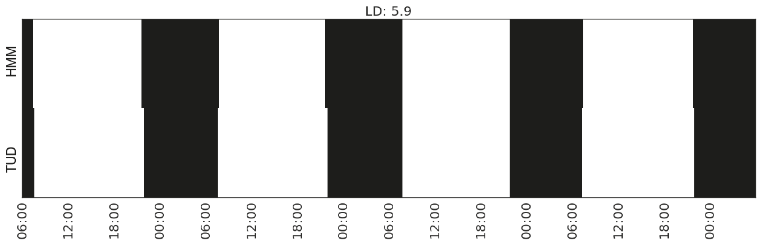
For the sleeping activity of Household 3, the best agreement is achieved by the feature capturing the gaps between the changes of movements in the living room. According to the interview data, we know that the living room is the geographical centre of the house, i.e., the passage to transit between kitchen, dining/study area and the sleeping area. The occupant keeps busy at home and spends a lot of time in the dining/study area and the living area.
For the activity of making hot drink, the feature identifying humidity changes in the utility room and bedroom of Household 3 is contained in the subset of features that achieves the best agreement. A further investigation of the time use diary shows that when making coffee in the kitchen in the mornings the occupant shaves in the bathroom which is located next to the utility room and bedroom. The humidity change in this case is very likely caused by the humid bathroom.
The overlaps between the subsets of features that achieve the best agreement in recognising activities of preparing meal and eating show the close relation between the two types of activities. This demonstrates that sensor insensitive activities may be recognised via sensor readings from their causal/correlated activities. In this case, the recognition of preparing meal can help recognise eating.
For the laundry activity, since we have an energy monitor attached to the washing machine of each household, it is expected that using the features capturing the energy consumption of the washing machine would achieves the best agreement. However, for Household 2, the feature subset that achieves the best agreement also contains the changes of the energy consumption of the kitchen appliances as well as that of the total energy consumption. A further investigation of the time use diary shows that when doing laundry the occupant quite often cooks or makes coffee around the same time. However, among the three households, the agreement between the HMM and the time use diary for laundry activity in Household 2 is the lowest, which may indicate the possibility of misreport or that the reported laundry activities involve other elements, such as sorting, hanging out, folding, etc.
Among the seven types of activities, listening to radio has the lowest agreement (the largest value in LD) between the detection from the sensor-generated data and the records in the time use diaries. In case of Household 2, the time use diary tells us that the occupant listens to radio in the bedroom while getting up, in the kitchen while preparing meals and in the dining area when having meals. Similarly, the occupant in Household 3 listens to radio in the kitchen when preparing meal and in the living room when relaxing. In both cases, the occupant is using more than one device for listening to radio in more than one place.
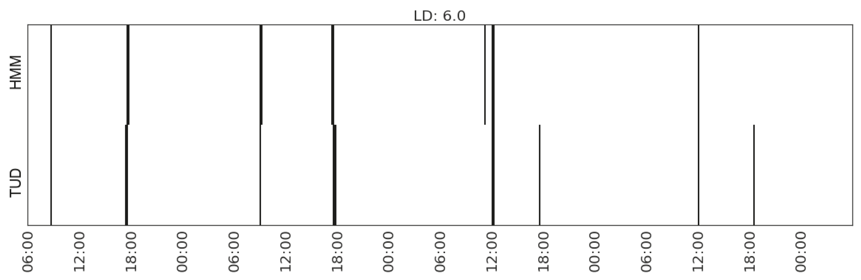
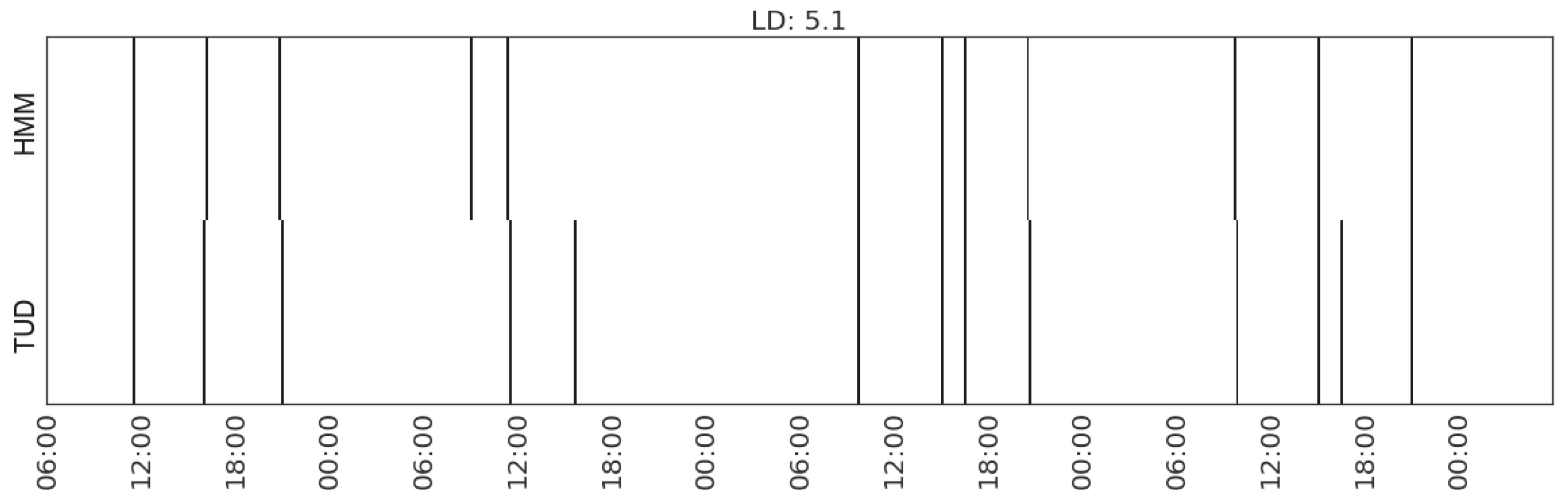
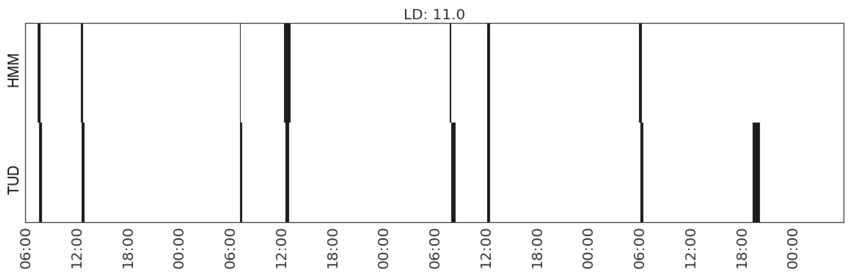
For illustration, we plot the comparison of each type of activity detected from the sensor data and that recorded in the time use diaries (Figure 12, Figure 13, Figure 14, Figure 15, Figure 16, Figure 17 and Figure 18). In each figure, the upper part shows the state sequences generated by an HMM using the specific set of features, and the lower part shows the activity sequences recorded in the time use diary (TUD). The black bins represent the time slices when a particular activity is detected/recorded.
The activity durations generated by the HMMs mostly overlap with those recorded in the time use diary, with some local shifts along the time line. The only exception in these seven plots is the activity of listening to radio in Household 2, which suggests that the features being used are not sufficient enough to distinguish the occurrences of such activities. In some cases, radio is used as background, which does not necessarily constitute the activity of listening to the radio.
7. Conclusions
In this paper, we presented a mixed-methods approach for recognising activities at home. In particular, we proposed a metric for evaluating the agreement between the predicted activities from models trained by the sensor data and the activities recorded in a time use diary. We also investigated ways of extracting and selecting features from sensor-generated data for activity recognition.
The focus of this work is not on improving the recognition performance of particular models but to present a framework for quantifying how activity recognition models trained by sensor-generated data can be evaluated on the basis of their agreement with activities recorded in time use diaries. We demonstrate the usefulness of this framework by an experiment involving three trial households. The evaluation results can provide evidence about which types of sensors are more effective for detecting certain types of activities in a household. This may further help researchers in understanding the occupant’s daily activities and the contexts in which certain activities occur. The agreement between the sensor-generated data and the time use diary may also help to validate the quality of the diary.
This is an on-going research, investigating the use of digital sensors for social research, using household practices as a testbed. As this is written, we are in the process of collecting data from three types of households: single occupant, families with children and ≥2 adults. There are several directions to consider for extending this work. We are adding a wearable wristband sensor to the setting to detect the proximity of participants to each sensor box via Bluetooth RSSI (received signal strength indicator). Such data will give us a more accurate reading of presence and co-presence of particular occupants in different parts of their home, while also helping us in obtaining more accurate start and end times of certain activities. We will continue to investigate other activity recognition methods and feature selection techniques. In addition, we are interested in employing post and assisted labelling mechanisms, for example, by asking participants to assign an agreement score to the activity sequences generated by our activity recognition models. In this way, another layer of agreement can be added to the evaluation.
References
Acknowledgments
The authors thank William Headley for the design and manufacture of the sensor box (also known as desk egg). The work was carried out as part of the “HomeSense: digital sensors for social research” project funded by the Economic and Social Research Council (grant ES/N011589/1) through the National Centre for Research Methods.
Author Contributions
All authors participated in refining the initial study. Jie Jiang and Riccardo Pozza designed the experiments; Jie Jiang performed the experiments and analysed the data; and Kristrún Gunnarsdóttir orchestrated the fieldwork and contributed materials. All authors discussed enhancements, results and implications, wrote the manuscript and commented on it at all stages.
Conflicts of Interest
The authors declare no conflict of interest. The founding sponsors had no role in the design of the study; in the collection, analyses, or interpretation of data; in the writing of the manuscript, and in the decision to publish the results.
References
- Ruppanner, L. Contemporary Family Issues; Oxford University Press: Oxford, UK, 2015. [Google Scholar]
- Atkinson, R.; Jacobs, K. House, Home and Society; Palgrave: London, UK, 2016. [Google Scholar]
- Gattshall, M.L.; Shoup, J.A.; Marshall, J.A.; Crane, L.A.; Estabrooks, P.A. Validation of a survey instrument to assess home environments for physical activity and healthy eating in overweight children. Int. J. Behav. Nutr. Phys. Act. 2008, 5, 1–13. [Google Scholar] [CrossRef] [PubMed]
- Williams, S.J.; Coveney, C.; Meadows, R. ‘M-apping’ sleep? Trends and transformations in the digital age. Sociol. Health Illn. 2015, 37, 1039–1054. [Google Scholar] [CrossRef] [PubMed]
- López, D.; Sánchez-Criado, T. Analysing Hands-on-Tech Care Work in Telecare Installations. Frictional Encounters with Gerontechnological Designs. In Aging and the Digital Life Course; Prendergast, D., Garattini, C., Eds.; Berghahn: New York, NY, USA, 2015; Chapter 9. [Google Scholar]
- Mort, M.; Roberts, C.; Callen, B. Ageing with telecare: care or coercion in austerity? Sociol. Health Illn. 2013, 35, 799–812. [Google Scholar] [CrossRef] [PubMed]
- Sullivan, O.; Gershuny, J. Change in Spousal Human Capital and Housework: A Longitudinal Analysis. Eur. Sociol. Rev. 2016, 32, 864–880. [Google Scholar] [CrossRef]
- Pierce, J.; Schiano, D.J.; Paulos, E. Home, Habits, and Energy: Examining Domestic Interactions and Energy Consumption. In Proceedings of the SIGCHI Conference on Human Factors in Computing Systems CHI ’10, Atlanta, GA, USA, 10–15 April 2010; pp. 1985–1994. [Google Scholar]
- Shannon-Baker, P. Making Paradigms Meaningful in Mixed Methods Research. J. Mixed Methods Res. 2016, 10, 319–334. [Google Scholar] [CrossRef]
- Ganong, L.; Coleman, M. Qualitative research on family relationships. J. Soc. Person. Relatsh. 2014, 31, 451–459. [Google Scholar] [CrossRef]
- British Social Attitudes Survey (33rd ed.). Available online: http://www.bsa.natcen.ac.uk/latest-report/british-social-attitudes-33/introduction.aspx (accessed on 30 March 2017).
- Office for National Statistic (UK). Available online: https://www.ons.gov.uk/ (accessed on 30 March 2017).
- Chenu, A.; Lesnard, L. Time Use Surveys: A Review of their Aims, Methods, and Results. Eur. J. Sociol. 2006, 47, 335–359. [Google Scholar] [CrossRef]
- Gershuny, J.; Harms, T.A. Housework Now Takes Much Less Time: 85 Years of US Rural Women’s Time Use. Soc. Forces 2016, 95, 503–524. [Google Scholar] [CrossRef]
- European Communities. Harmonised European Time Use Surveys: 2008 Guidelines; Eurostat Methodologies and Working Papers; Population and social conditions; European Communities: Luxembourg, 2009. [Google Scholar]
- Kelly, P.; Thomas, E.; Doherty, A.; Harms, T.; Burke, O.; Gershuny, J.; Foster, C. Developing a Method to Test the Validity of 24 Hour Time Use Diaries Using Wearable Cameras: A Feasibility Pilot. PLOS ONE 2015, 10, 1–15. [Google Scholar] [CrossRef] [PubMed]
- Benmansour, A.; Bouchachia, A.; Feham, M. Multioccupant Activity Recognition in Pervasive Smart Home Environments. ACM Comput. Surv. 2015, 48, 34:1–34:36. [Google Scholar] [CrossRef]
- Poppe, R. A survey on vision-based human action recognition. Image Vis. Comput. 2010, 28, 976–990. [Google Scholar] [CrossRef]
- Lara, O.D.; Labrador, M.A. A Survey on Human Activity Recognition using Wearable Sensors. IEEE Commun. Surv. Tutor. 2013, 15, 1192–1209. [Google Scholar] [CrossRef]
- Shoaib, M.; Bosch, S.; Incel, O.D.; Scholten, H.; Havinga, P.J. A Survey of Online Activity Recognition Using Mobile Phones. Sensors 2015, 15, 2059–2085. [Google Scholar] [CrossRef] [PubMed]
- Amft, O.; Tröster, G. Recognition of dietary activity events using on-body sensors. Artif. Intell. Med. 2008, 42, 121–136. [Google Scholar] [CrossRef] [PubMed]
- Wang, J.; Zhang, Z.; Li, B.; Lee, S.; Sherratt, R.S. An enhanced fall detection system for elderly person monitoring using consumer home networks. IEEE Trans. Consum. Electron. 2014, 60, 23–29. [Google Scholar] [CrossRef]
- Lin, Z.H.; Fu, L.C. Multi-user Preference Model and Service Provision in a Smart Home Environment. In Proceedings of the 2007 IEEE International Conference on Automation Science and Engineering, Scottsdale, AZ, USA, 22–25 September 2007; pp. 759–764. [Google Scholar]
- van Kasteren, T.L.M.; Englebienne, G.; Kröse, B.J.A. Human Activity Recognition from Wireless Sensor Network Data: Benchmark and Software. In Activity Recognition in Pervasive Intelligent Environments; Chen, L., Nugent, C.D., Biswas, J., Hoey, J., Eds.; Atlantics Press: Amsterdam, The Netherland, 2011; pp. 165–186. [Google Scholar]
- Hsu, K.C.; Chiang, Y.T.; Lin, G.Y.; Lu, C.H.; Hsu, J.Y.J.; Fu, L.C. Strategies for Inference Mechanism of Conditional Random Fields for Multiple-Resident Activity Recognition in a Smart Home. In Trends in Applied Intelligent Systems, Proceedings of the 23rd International Conference on Industrial Engineering and Other Applications of Applied Intelligent Systems, Cordoba, Spain, 1–4 June 2010; García-Pedrajas, N., Herrera, F., Fyfe, C., Benítez, J.M., Ali, M., Eds.; Springer: Berlin/Heidelberg, Germany, 2010; pp. 417–426. [Google Scholar]
- Fan, X.; Zhang, H.; Leung, C.; Miao, C. Comparative study of machine learning algorithms for activity recognition with data sequence in home-like environment. In Proceedings of the 2016 IEEE International Conference on Multisensor Fusion and Integration for Intelligent Systems (MFI), Baden-Baden, Germany, 19–21 September 2016; pp. 168–173. [Google Scholar]
- Cook, D.J.; Crandall, A.; Singla, G.; Thomas, B. Detection of Social Interaction in Smart Spaces. Cybern. Syst. 2010, 41, 90–104. [Google Scholar] [CrossRef] [PubMed]
- Silverman, D. Interpreting Qualitative Data: Methods for Analyzing Talk, Text and Interaction, 3rd ed.; SAGE Publications: Thousand Oaks, CA, USA, 2006. [Google Scholar]
- Wang, L.; Gu, T.; Tao, X.; Chen, H.; Lu, J. Recognizing multi-user activities using wearable sensors in a smart home. Pervasive Mob. Comput. 2011, 7, 287–298. [Google Scholar] [CrossRef]
- Cheng, Y. Mean Shift, Mode Seeking, and Clustering. IEEE Trans. Pattern Anal. Mach. Intell. 1995, 17, 790–799. [Google Scholar] [CrossRef]
- Picard, D. Testing and estimating change-points in time series. Adv. Appl. Probab. 1985, 17, 841–867. [Google Scholar] [CrossRef]
- Hall, M.A.; Smith, L.A. Feature Selection for Machine Learning: Comparing a Correlation-Based Filter Approach to the Wrapper. In Proceedings of the Twelfth International Florida Artificial Intelligence Research Society Conference, San Francisco, CA, USA, 1–5 May 1999; AAAI Press: Palo Alto, CA, USA, 1999; pp. 235–239. [Google Scholar]
- Levenshtein, V.I. Binary codes capable of correcting deletions, insertions, and reversals. Cybern. Control Theory 1966, 10, 707–710. [Google Scholar]
- Jiang, J.; Pozza, R.; Gunnarsdóttir, K.; Gilbert, N.; Moessner, K. Recognising Activities at Home: Digital and Human Sensors. In Proceedings of the International Conference on Future Networks and Distributed Systems ICFNDS ’17, Cambridge, UK, 19–20 July 2017; ACM: New York, NY, USA, 2017; pp. 17:1–17:11. [Google Scholar]
- Cook, D.J.; Youngblood, M.; Heierman, E.O.; Gopalratnam, K.; Rao, S.; Litvin, A.; Khawaja, F. MavHome: An agent-based smart home. In Proceedings of the First IEEE International Conference on Pervasive Computing and Communications, Fort Worth, TX, USA, 23–26 March 2003; pp. 521–524. [Google Scholar]
- Cook, D.J.; Schmitter-edgecombe, M.; Crandall, A.; Sanders, C.; Thomas, B. Collecting and Disseminating Smart Home Sensor Data in the CASAS Project. In Proceedings of the CHI Workshop on Developing Shared Home Behavior Datasets to Advance HCI and Ubiquitous Computing Research, Boston, MA, USA, 4–9 April 2009. [Google Scholar]
- Singla, G.; Cook, D.J.; Schmitter-Edgecombe, M. Recognizing independent and joint activities among multiple residents in smart environments. J. Ambient Intell. Humaniz. Comput. 2010, 1, 57–63. [Google Scholar] [CrossRef] [PubMed]
- Chiang, Y.T.; Hsu, K.C.; Lu, C.H.; Fu, L.C.; Hsu, J.Y.J. Interaction models for multiple-resident activity recognition in a smart home. In Proceedings of the 2010 IEEE/RSJ International Conference on Intelligent Robots and Systems, Taipei, Taiwan, 18–22 October 2010; pp. 3753–3758. [Google Scholar]
- Fatima, I.; Fahim, M.; Lee, Y.K.; Lee, S. A Unified Framework for Activity Recognition-Based Behavior Analysis and Action Prediction in Smart Homes. Sensors 2013, 13, 2682–2699. [Google Scholar] [CrossRef] [PubMed]
- Fang, H.; He, L.; Si, H.; Liu, P.; Xie, X. Human activity recognition based on feature selection in smart home using back-propagation algorithm. ISA Trans. 2014, 53, 1629–1638. [Google Scholar] [CrossRef] [PubMed]
- Krishnan, N.C.; Cook, D.J. Activity Recognition on Streaming Sensor Data. Pervasive Mob. Comput. 2014, 10, 138–154. [Google Scholar] [CrossRef] [PubMed]
- Dawadi, P.N.; Cook, D.J.; Schmitter-Edgecombe, M. Modeling Patterns of Activities Using Activity Curves. Pervasive Mob. Comput. 2016, 28, 51–68. [Google Scholar] [CrossRef] [PubMed]
- Alemdar, H.; Ertan, H.; Incel, O.D.; Ersoy, C. ARAS human activity datasets in multiple homes with multiple residents. In Proceedings of the 2013 7th International Conference on Pervasive Computing Technologies for Healthcare and Workshops, Venice, Italy, 5–8 May 2013; pp. 232–235. [Google Scholar]
- Prossegger, M.; Bouchachia, A. Multi-resident Activity Recognition Using Incremental Decision Trees. In Proceedings of the Third International Conference ICAIS 2014 Adaptive and Intelligent Systems, Bournemouth, UK, 8–10 September 2014; Bouchachia, A., Ed.; Springer: Cham, Switzerland, 2014; pp. 182–191. [Google Scholar]
- Kröse, B.; Kasteren, T.V.; Gibson, C.; Dool, T.V.D. Care: Context awareness in residences for elderly. In Proceedings of the Conference of the International Society for Gerontechnology, Pisa, Italy, 21–25 June 2008. [Google Scholar]
- van Kasteren, T.; Noulas, A.; Englebienne, G.; Kröse, B. Accurate Activity Recognition in a Home Setting. In Proceedings of the 10th International Conference on Ubiquitous Computing UbiComp ’08, Seoul, Korea, 21–24 September 2008; pp. 1–9. [Google Scholar]
- Nez, F.J.O.; Englebienne, G.; de Toledo, P.; van Kasteren, T.; Sanchis, A.; Kröse, B. In-Home Activity Recognition: Bayesian Inference for Hidden Markov Models. IEEE Pervasive Comput. 2014, 13, 67–75. [Google Scholar]
- Singh, D.; Merdivan, E.; Psychoula, I.; Kropf, J.; Hanke, S.; Geist, M.; Holzinger, A. Human Activity Recognition Using Recurrent Neural Networks. In Machine Learning and Knowledge Extraction: First IFIP TC 5, WG 8.4, 8.9, 12.9, Proceedings of the International Cross-Domain Conference, CD-MAKE 2017, Reggio, Italy, 29 August–1 September 2017; Holzinger, A., Kieseberg, P., Tjoa, A.M., Weippl, E., Eds.; Springer: Berlin, Germany, 2017; pp. 267–274. [Google Scholar]
- Laput, G.; Zhang, Y.; Harrison, C. Synthetic Sensors: Towards General-Purpose Sensing. In Proceedings of the 2017 CHI Conference on Human Factors in Computing Systems, Denver, CO, USA, 6–11 May 2017; ACM: New York, NY, USA, 2017; pp. 3986–3999. [Google Scholar]
- Seeeduino Arch-Pro. Available online: https://developer.mbed.org/platforms/Seeeduino-Arch-Pro (accessed on 30 March 2017).
- SparkFun Humidity and Temperature Sensor Breakout—HTU21D. Available online: https://www.sparkfun.com/products/retired/12064 (accessed on 30 March 2017).
- SparkFun RGB and Gesture Sensor—APDS-9960. Available online: https://www.sparkfun.com/products/12787 (accessed on 30 March 2017).
- Pololu Carrier with Sharp GP2Y0A60SZLF Analog Distance Sensor. Available online: https://www.pololu.com/product/2474 (accessed on 30 March 2017).
- SparkFun MEMS Microphone Breakout—INMP401 (ADMP401). Available online: https://www.sparkfun.com/products/9868 (accessed on 30 March 2017).
- Current Cost—Individual Appliance Monitor (IAM). Available online: http://www.currentcost.com/product-iams.html (accessed on 30 March 2017).
- Pedregosa, F.; Varoquaux, G.; Gramfort, A.; Michel, V.; Thirion, B.; Grisel, O.; Blondel, M.; Prettenhofer, P.; Weiss, R.; Dubourg, V.; et al. Scikit-learn: Machine learning in Python. J. Mach. Learn. Res. 2011, 12, 2825–2830. [Google Scholar]
- Killick, R.; Fearnhead, P.; Eckley, I.A. Optimal Detection of Changepoints with a Linear Computational Cost. J. Am. Stat. Assoc. 2012, 107, 1590–1598. [Google Scholar] [CrossRef]
- Killick, R.; Eckley, I.A. Changepoint: An R package for changepoint analysis. J. Stat. Softw. 2014, 58, 1–19. [Google Scholar] [CrossRef]
- Guyon, I.; Elisseeff, A. An Introduction to Variable and Feature Selection. J. Mach. Learn. Res. 2003, 3, 1157–1182. [Google Scholar]
- Ghiselli, E.E. Theory of Psychological Measurement; McGraw-Hill: New York, NY, USA, 1964. [Google Scholar]
- Press, W.H.; Flannery, B.P.; Teukolski, S.A.; Vetterling, W.T. Numerical Recipes in C; Cambridge University Press: Cambridge, UK, 1988. [Google Scholar]
- Quinlan, J.R. Programs for Machine Learning; Morgan Kaufmann: Burlington, MA, USA, 1993. [Google Scholar]
- Li, J.; Cheng, K.; Wang, S.; Morstatter, F.; Trevino, R.P.; Tang, J.; Liu, H. Feature Selection: A Data Perspective. arXiv 2016, arXiv:1601.07996. [Google Scholar] [CrossRef]
- Zucchini, W.; MacDonald, I.L. Hidden Markov Models for Time Series: An Introduction Using R; CRC Press: Boca Raton, FL, USA, 2009. [Google Scholar]
- Hmmlearn. Available online: http://hmmlearn.readthedocs.io/ (accessed on 30 March 2017).
- Weighted-Levenshtein. Available online: http://weighted-levenshtein.readthedocs.io/ (accessed on 30 March 2017).
Figure 1.
Sensor Modules: (a) Sensor Box; and (b) Electricity Monitor.

Figure 2.
Demonstration Interface.

Figure 3.
Mean shift clustering of range readings from a sensor box in the living room (with dining space) of Household 1.
Figure 3.
Mean shift clustering of range readings from a sensor box in the living room (with dining space) of Household 1.

Figure 4.
Mean shift clustering of noise-level readings from a sensor box in the living room (with dining space) of Household 1.
Figure 4.
Mean shift clustering of noise-level readings from a sensor box in the living room (with dining space) of Household 1.

Figure 5.
Change points of temperature readings from a sensor box in the kitchen of Household 2.
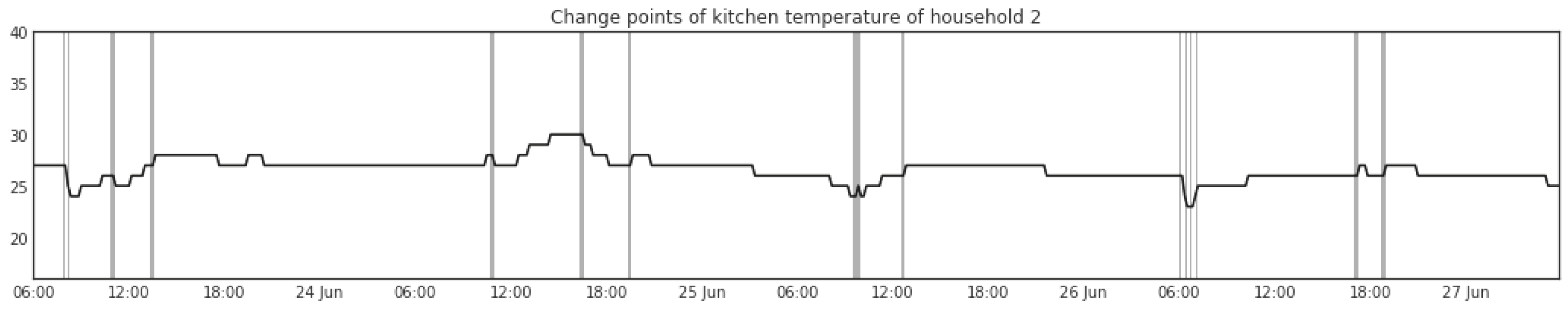
Figure 6.
Change points of humidity readings from a sensor box in the kitchen of Household 2.
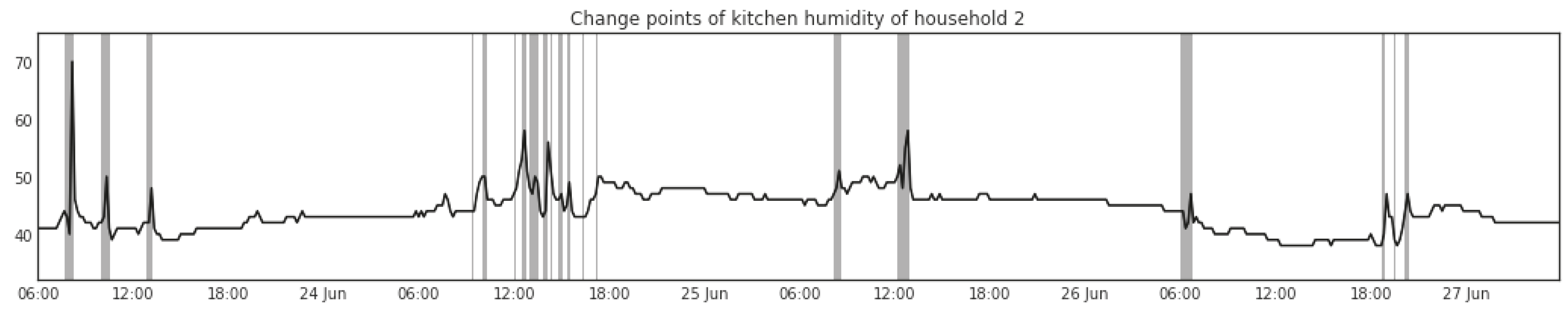
Figure 7.
Gaps between change points in the electricity readings from the CT clamp connected to the electricity main of Household 3.
Figure 7.
Gaps between change points in the electricity readings from the CT clamp connected to the electricity main of Household 3.

Figure 8.
Gaps between change points in the brightness readings from the sensor box in the bedroom of Household 3.
Figure 8.
Gaps between change points in the brightness readings from the sensor box in the bedroom of Household 3.

Figure 9.
Correlations between the features of temperature and range readings from two sensor boxes installed in the kitchen of Household 1.
Figure 9.
Correlations between the features of temperature and range readings from two sensor boxes installed in the kitchen of Household 1.

Figure 10.
Correlations between the activities recorded by the occupant from Household 3 and the features of electricity consumption.
Figure 10.
Correlations between the activities recorded by the occupant from Household 3 and the features of electricity consumption.
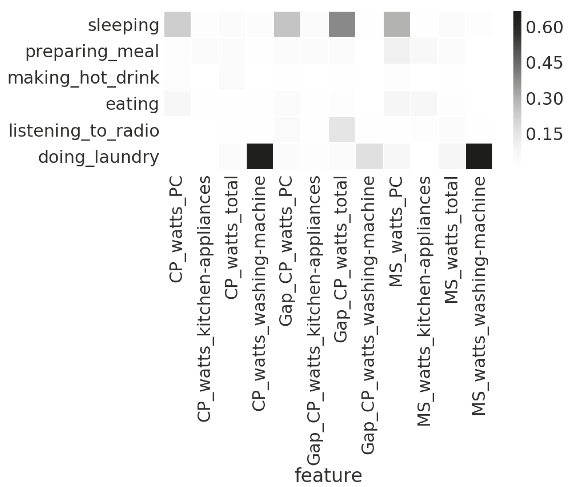
Figure 11.
Graphical representation of a Hidden Markov Model.
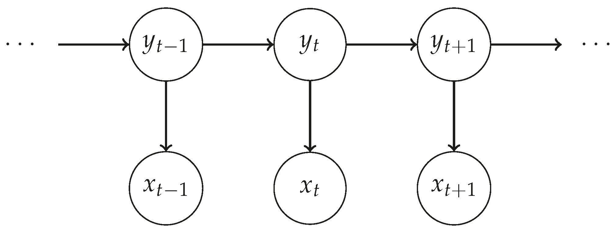
Figure 12.
Recognising the activity of preparing meal in Household 1 with feature set (MS_watts_total, MS_watts_microwave).
Figure 12.
Recognising the activity of preparing meal in Household 1 with feature set (MS_watts_total, MS_watts_microwave).

Figure 13.
Recognising the activity of making hot drink in Household 1 with feature set (MS_watts_kitchen-appliances).
Figure 13.
Recognising the activity of making hot drink in Household 1 with feature set (MS_watts_kitchen-appliances).

Figure 14.
Recognising the activity of eating in Household 2 with feature set (MS_watts_kitchen-appliances, MS_range_living/dining-room(2)).
Figure 14.
Recognising the activity of eating in Household 2 with feature set (MS_watts_kitchen-appliances, MS_range_living/dining-room(2)).

Figure 15.
Recognising the activity of listening to radio in Household 2 with feature set (CP_range_hallway, MS_watts_kitchen-appliances, MS_range_bedroom).
Figure 15.
Recognising the activity of listening to radio in Household 2 with feature set (CP_range_hallway, MS_watts_kitchen-appliances, MS_range_bedroom).
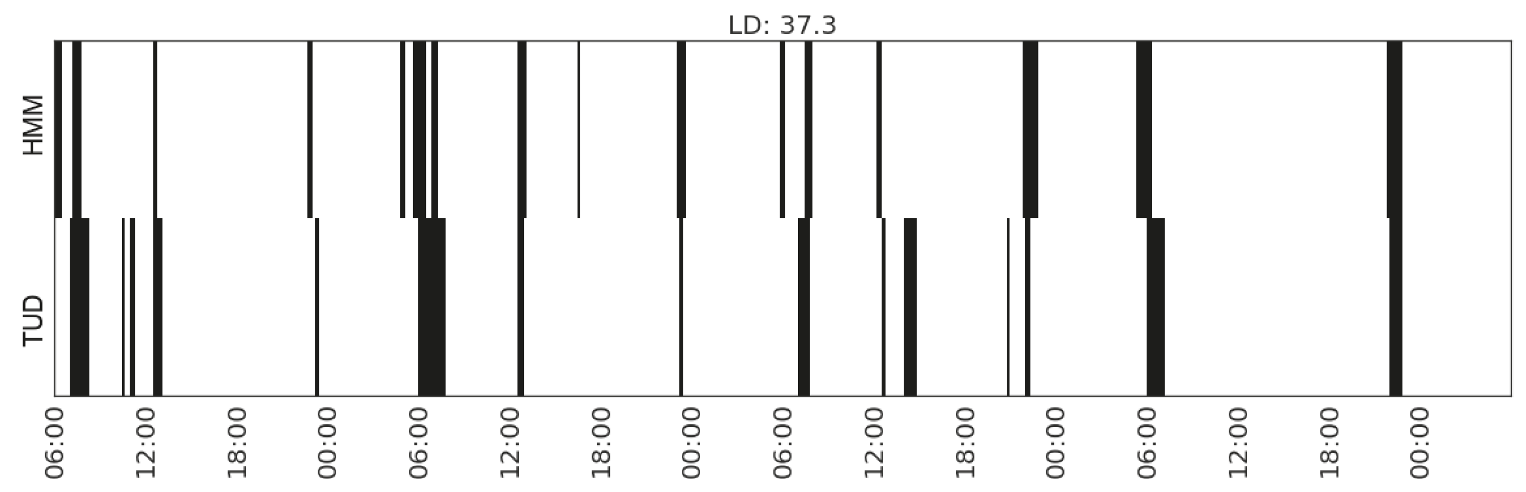
Figure 16.
Recognising the activity of watching TV in Household 2 with feature set (MS_watts_TV).
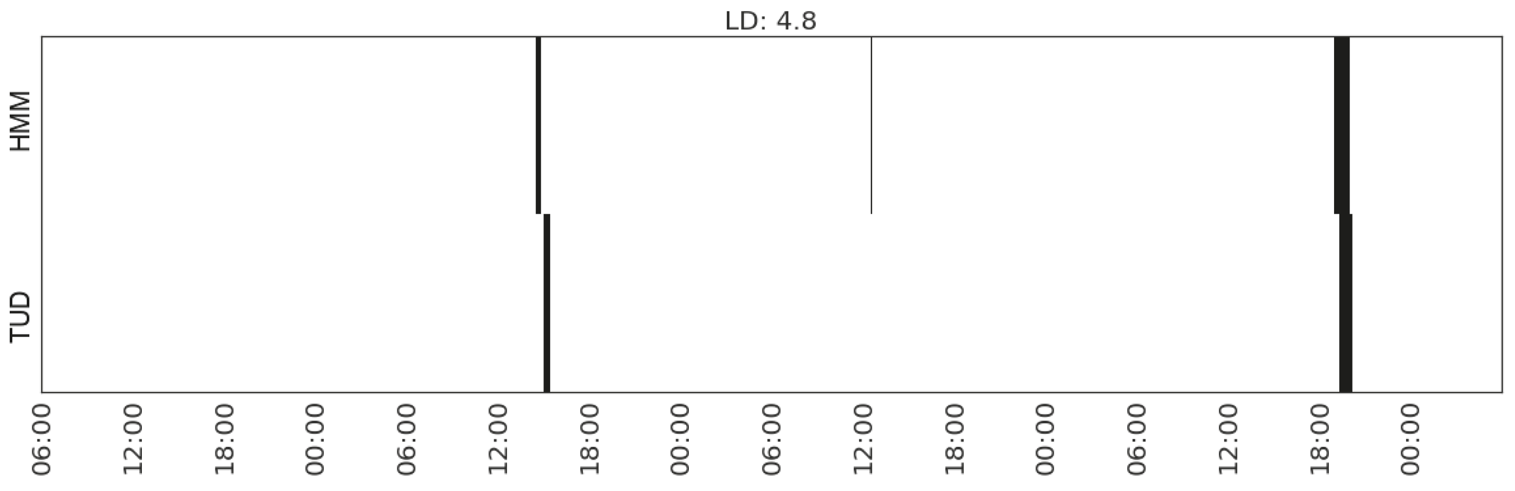
Figure 17.
Recognising the activity of doing laundry in Household 3 with feature set (MS_watts_washing-machine, CP_watts_washing-machine).
Figure 17.
Recognising the activity of doing laundry in Household 3 with feature set (MS_watts_washing-machine, CP_watts_washing-machine).
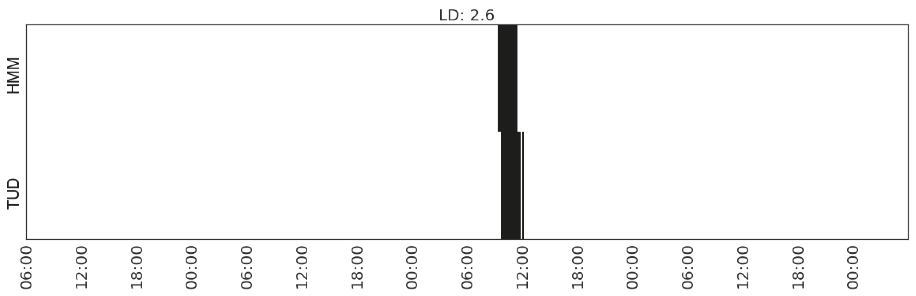
Figure 18.
Recognising the activity of sleeping in Household 3 with feature set (Gap_CP_range_living-room).
Figure 18.
Recognising the activity of sleeping in Household 3 with feature set (Gap_CP_range_living-room).

Table 1.
Sensor Modules
| Sensor Modules | Measurement | |
|---|---|---|
| Sensor Box | Temperature sensor | °C |
| Humidity sensor | % | |
| Light Sensor | ||
| Ranging sensor | cm | |
| Microphone | dB SPL | |
| Energy monitor | watts | |
Table 2.
Sensors installed in each trial home.
| Household | Rooms | Sensor Boxes (Location Installed) | Electricity Monitors (Appliances Attached) |
|---|---|---|---|
| 1 | Master bedroom | Next to bed | |
| Guest bedroom | Next to bed | Teasmade | |
| Kitchen | Entrance; Food preparation area | Washing machine; Microwave; Kettle | |
| Living room with dining space | Entrance; Sitting area | TV | |
| Living room | Sitting area | ||
| Hallway | On the wall | ||
| 2 | Bedroom | Next to bed | |
| Kitchen | Cooking area | Washing machine; Kettle, Toaster, Bread maker | |
| Living room with dining space | Dining area; Sitting area | TV; Ironing/Vacuum | |
| Living room | Sitting area | Laptop | |
| Study | Book shelf | ||
| Hallway | On the wall | ||
| 3 | Bedroom | Next to bed | |
| Kitchen | Food preparation area; Cooking area | Washing machine; Kettle, Toaster | |
| Dining room combined with study | Sitting area; Next to desktop computer | Desktop computer | |
| Living room | Sitting area | ||
| First utility room | Near entrance | ||
| Second utility room | Near entrance | ||
| Hallway | On the wall | Vacuum cleaner |
Table 3.
Sensor Data Set Statistics.
| Household | Sensor Boxes | Energy Monitors | Total |
|---|---|---|---|
| 1 | |||
| 2 | |||
| 3 |
Table 4.
Time use diary example.
| Time | Primary Activity | Secondary Activity | Location | Devices |
|---|---|---|---|---|
| 08:00–08:10 | Preparing meal | Listening to radio | Kitchen | Kettle, Radio |
| 08:10–08:20 | Eating | Watching TV | Living room | TV |
| ⋮ | ⋮ | ⋮ | ⋮ | ⋮ |
| 18:00–18:10 | Preparing meal | ─── | Kitchen | Oven |
| 18:10–18:20 | Preparing meal | ─── | Kitchen | Oven |
Table 5.
Number of occurrences and time spent for each type of activity in the data set.
| Activity | Household 1 | Household 2 | Household 3 | |||
|---|---|---|---|---|---|---|
| Number of Occurrences | Percentage of Time | Number of Occurrences | Percentage of Time | Number of Occurrences | Percentage of Time | |
| Sleeping | 5 | 36.94% | 5 | 31.08% | 5 | 40.28% |
| Preparing meal | 8 | 2.08% | 10 | 2.78% | 7 | 3.47% |
| Making hot drink | 13 | 2.26% | 11 | 1.91% | 2 | 0.52% |
| Eating | 10 | 4.17% | 8 | 3.65% | 8 | 3.30% |
| Watching TV | 13 | 16.15% | 2 | 1.39% | / | / |
| Listening to radio | / | / | 15 | 10.42% | 6 | 17.88% |
| Doing Laundry | 1 | 0.17% | 6 | 1.04% | 2 | 2.43% |
Table 6.
Pearson correlation between the readings from pairs of sensors placed in the same room.
| Sensor Reading | Temperature | Humidity | Light | Range | Sound |
|---|---|---|---|---|---|
| Household 1 (kitchen) | 0.94 | 0.75 | 0.90 | 0.56 | 0.88 |
| Household 1 (living/dining room) | 0.93 | 0.89 | 0.95 | 0.21 | 0.86 |
| Household 2 (living/dining room) | 0.49 | 0.62 | 0.85 | 0.33 | 0.57 |
| Household 3 (kitchen) | 0.90 | 0.92 | 0.97 | 0.29 | 0.80 |
| Household 3 (dining room/study) | 0.83 | 0.90 | 0.71 | 0.20 | 0.57 |
Table 7.
Feature sets achieve best agreement with respect to the seven types of activities.
| Household | Activities | Feature Sets | LD |
|---|---|---|---|
| 1 | Sleeping | (MS_light_living/dining-room, Gap_CP_light_bedroom) | 11.9 |
| Preparing meal | (MS_watts_total, MS_watts_microwave) | 6.0 | |
| Making hot drink | (MS_watts_kitchen-appliances) | 5.1 | |
| Eating | (MS_watts_total) | 17.0 | |
| Watching TV | (MS_watts_TV) | 16.6 | |
| Doing laundry | (MS_watts_washing-machine) | 0.7 | |
| 2 | Sleeping | (CP_light_kitchen(1), CP_light_bedroom, MS_temperature_living/dining-room(2)) | 16.7 |
| Preparing meal | (MS_watts_kitchen-appliances) | 11.2 | |
| Making hot drink | (MS_sound_kitchen(1)) | 11.6 | |
| Eating | (MS_watts_kitchen-appliances, MS_range_living/dining-room(2)) | 11.0 | |
| Watching TV | (MS_watts_TV) | 4.8 | |
| Listening to radio | (CP_range_hallway, MS_watts_kitchen-appliances, MS_range_bedroom) | 37.3 | |
| Doing laundry | (CP_watts_total, CP_watts_kitchen-appliances, CP_watts_washing-machine) | 12.1 | |
| 3 | Sleeping | (Gap_CP_range_living-room) | 5.9 |
| Preparing meal | (MS_range_kitchen(2), MS_watts_PC) | 26.1 | |
| Making hot drink | (CP_humidity_second-utility, CP_temperature_kitchen(2), CP_humidity_bedroom) | 1.7 | |
| Eating | (MS_range_kitchen(2), CP_temperature_dining-room/study(1)) | 16.0 | |
| Listening to radio | (MS_sound_living-room) | 37.2 | |
| Doing laundry | (MS_watts_washing-machine, CP_watts_washing-machine) | 2.6 |
© 2017 by the authors. Licensee MDPI, Basel, Switzerland. This article is an open access article distributed under the terms and conditions of the Creative Commons Attribution (CC BY) license (http://creativecommons.org/licenses/by/4.0/).
Share and Cite
MDPI and ACS Style
Jiang, J.; Pozza, R.; Gunnarsdóttir, K.; Gilbert, N.; Moessner, K. Using Sensors to Study Home Activities. J. Sens. Actuator Netw. 2017, 6, 32. https://doi.org/10.3390/jsan6040032
AMA Style
Jiang J, Pozza R, Gunnarsdóttir K, Gilbert N, Moessner K. Using Sensors to Study Home Activities. Journal of Sensor and Actuator Networks. 2017; 6(4):32. https://doi.org/10.3390/jsan6040032
Chicago/Turabian StyleJiang, Jie, Riccardo Pozza, Kristrún Gunnarsdóttir, Nigel Gilbert, and Klaus Moessner. 2017. "Using Sensors to Study Home Activities" Journal of Sensor and Actuator Networks 6, no. 4: 32. https://doi.org/10.3390/jsan6040032
Note that from the first issue of 2016, this journal uses article numbers instead of page numbers. See further details here.