Structural Panel VARs

Department of Economics, Schapiro Hall, 124 Hopkins Hall Dr., Williams College, Williamstown, MA 01267, USA
Econometrics 2013, 1(2), 180-206; https://doi.org/10.3390/econometrics1020180
Submission received: 30 May 2013
/
Revised: 6 August 2013
/
Accepted: 20 August 2013
/
Published: 24 September 2013
(This article belongs to the Special Issue Panel Time Series Methods)
Abstract
:The paper proposes a structural approach to VAR analysis in panels, which takes into account responses to both idiosyncratic and common structural shocks, while permitting full cross member heterogeneity of the response dynamics. In the context of this structural approach, estimation of the loading matrices for the decomposition into idiosyncratic versus common shocks is straightforward and transparent. The method appears to do remarkably well at uncovering the properties of the sample distribution of the underlying structural dynamics, even when the panels are relatively short, as illustrated in Monte Carlo simulations. Finally, these simulations also illustrate that the SVAR panel method can be used to improve inference, not only for properties of the sample distribution, but also for dynamics of individual members of the panel that lack adequate data for a conventional time series SVAR analysis. This is accomplished by using fitted cross sectional regressions of the sample of estimated panel responses to correlated static measures, and using these to interpolate the member-specific dynamics.
1. Introduction
Structural VAR analysis has become a widely used tool among empirical researchers, particularly for those interested in studying the underlying dynamic relationships among economic variables. Unfortunately, as is all too often the case, there are many areas of research for which the underlying approach of structurally identified VAR analysis is well suited for the questions that are deemed pertinent, but time series data of sufficient length for reliable inference are simply lacking. In this paper, we investigate whether a panel approach to structural VAR analysis can help to remedy this dilemma.
In particular, we are interested to learn whether the cross-sectional variation that is present in a panel can serve to compensate for the lack of temporal data available for individual members of the panel. In this regard, we are interested to learn not only whether the panel structure can serve to uncover median relationships for the sample despite the shortness of the time series, but also whether it can serve to improve the member-specific inference for any one member of the panel for which the time series data is too short for reliable time series analysis.
In doing so, we must account for two important features that are likely to characterize such panels. The first is that substantial heterogeneity is likely present across the individual members of the panel. This heterogeneity is not likely to be limited to simple fixed effects as is characteristic of conventional micro panel approaches, but rather is likely to extend to all of the dynamics as well, as is characteristic of more recent macro panel time series literature. Secondly, we must account for the cross-sectional dependence that is likely to arise from the fact that individual members of the panel are responding not only to their own member-specific idiosyncratic shocks, but also to shocks that are common across members of the panel.
Toward that end, we propose here a new approach to VAR analysis in panels which is based on a structural decomposition of shocks into common type shocks versus idiosyncratic type shocks, as well as into the component shocks within each of these types. In light of our allowance for complete heterogeneity of the dynamics among members of the panel, it is not a-priori obvious that the panel approach will outperform pure time series-based methods with similarly short series lengths. However, in our Monte Carlo simulations, we demonstrate that the method can perform remarkably well in recovering the underlying structural shocks and dynamics, and substantially outperforms corresponding time series methods. This is true even when the object of interest is analysis of the structural shocks and dynamics of a single member of the panel, rather than properties of the distribution of the full sample of member estimates, such as the panel mean or median, provided that country-specific correlates are available for the distribution of responses.
Accordingly, the panel approach that we propose here should be applicable to a wide range of panel data types, including but not limited to panels composed of multi-country or multi-regional data, panels composed of disaggregated market data or, indeed, even firm level or household level data. In short the technique is viable for any panel that includes a time series dimension that is of sufficient length to at least minimally estimate member-specific VAR coefficients. Furthermore, the method is appropriate for unbalanced panels for which the data span differs by member of the panel.
To be clear, there have been other approaches to the analysis of VARs in panels. Early examples include the work of Holz-Eakin, Newey and Rosen [8]. However, the approach used in these early works, including the dynamic panel literature that followed with the works of Arellano and Bond [1] and many others, are subject to the well-known critique associated with latent heterogeneity in lagged dependent variables leading to inconsistent estimation, which makes the approach of the dynamic panel literature not well suited to panels with heterogenous dynamics. A good reference for this critique is the work of Pesaran and Smith [16].
Other, more recent approaches to VARs in panels include the Bayesian VAR methods of Canova and Ciccarelli [5],[6]. This method allows for time varying parameters and models the cross-sectional dependence in terms of a factor model and uses a Bayesian approach to estimation in order to deal with the large number of parameters, with an emphasis on the responses of individual members to functions of the observable variables. However, the approach is fundamentally a reduced form approach in that members of the panel are responding to innovations in the observables, with no attempt to recover structural shocks or dynamics.
Another approach is the Global VAR analysis of Pesaran, Schuermann and Weiner [15]. They use a reduced form VECM framework to model the individual member responses to specific observed foreign global variables, such as U.S. economic data, as well as the member-specific data in terms of non-orthoganized generalized impulse responses.
What is distinct about the method proposed in this paper is that we take a fully structural approach, with impulse responses based on orthogonalized structural shocks and structural identifying restrictions on the dynamics. In this regard, the approach developed in this paper is more in keeping with the traditional time series structural VAR literature, such as Bernanke [2], Blanchard and Quah [3], Blanchard and Watson [4], Clarida and Gali [7], Sims [17] and the many others that have followed this line of research. As we will see, this structural approach when adapted to a heterogeneous panel framework allows for relatively straightforward estimation of the loading vectors, which decompose the structural shocks into common versus idiosyncratic shocks. This, in turn, facilitates a direct and transparent structural interpretation of the estimates. As we will illustrate by Monte Carlo simulation, the small sample properties of such an approach provide an attractive opportunity for researchers faced with relatively short data series.
The remainder of the paper is organized as follows. In the next Section, 2, we describe the panel data generating process and the econometrics of identification and estimation of the structural shocks and associated impulse responses. In Section 3, we study by Monte Carlo simulation the small sample performance of the technique. Section 4 offers concluding remarks.1
2. Representation of Model Dynamics and Estimation
In this section, we describe both the data generating process and the econometric estimation and identification of the structural dynamics of the panel. The key to our estimation and identification method will be the assumption that a model representation exists that builds upon structural shocks that can be decomposed into both common and idiosyncratic structural shocks, which are mutually orthogonal.
Thus, for the data generating process, we consider a panel composed of individual members, each of which consists of an vector of observed endogenous variables, , for , . Since the panel may be unbalanced, the data are assumed to be observed over time periods. To accommodate fixed effects and to simplify the notation in our treatment, we will consider the vector of demeaned data, , where , with .
Driving the temporal variations in these data are the unobserved structural shocks. In particular, we consider an vector of composite white noise shocks , , for each member, i, of the panel. These composite shocks are distributed independently over time, but may be cross-sectionally-dependent.
In particular, we consider a common factor representation for this dependence, such that , where the two categories of mutually orthogonal structural shocks, and , represent, respectively, the member-specific idiosyncratic white noise structural shocks and the common white noise structural shocks shared by all members of the panel, and are the member-specific loading coefficients for the common shocks.2
In keeping with the structural VAR literature, the structural shocks are assumed to be orthogonal with respect to each other for each type, so that the various idiosyncratic shocks are mutually orthogonal to one another, as are the various common shocks to one another. Furthermore, in keeping with the structural VAR literature, the variances of these unobserved shocks are taken to be arbitrarily normalizable. Accordingly, if we imagine stacking the vector on top of the vectors for each member, i, then the corresponding vector would have a covariance matrix for each i with the first diagonal elements corresponding to the variances of the , the next diagonal elements corresponding to the variances of the and all off diagonal elements equal to zero.
We collect and summarize these various assumptions in the following statement.
Structural Shock Representation. Associated with the vector of demeaned panel data, , let where and are vectors of common and idiosyncratic white noise shocks respectively. Let be an diagonal matrix such that the diagonal elements are the loading coefficients , . Then
These restrictions are analogous to those made in the time series structural VAR literature and are a natural extension of those restrictions as applied to the panel setting. Furthermore, notice that the above conditions imply that the covariance matrix for the composite white noise errors, , is such that is also a diagonal covariance matrix with arbitrarily normalizable variances subject to the adding up constraint implied by Equation (1). This ensures that the restrictions that are made for the panel become consistent with similar restrictions made upon the individual data if they were treated as individual time series rather than as members of a panel.
Next, we turn to the representation of the model dynamics in response to these shocks. To facilitate the notation for the concurrent discussion of both the short run and long run identifying restrictions on the dynamics, we will take the stationary form to be in terms of the differences of the demeaned variables, namely . Consequently, by the Wold representation theorem, we know that a moving average representation exists for the composite errors, such that , where , which is subject to the usual square summability condition as .
Similarly, we can use time effects to describe the components of that are common to all members of the panel and use a moving average representation to describe the response of these to the common shocks. Specifically, let be the vector of common time effects, where we have used a t subscript on the value of to reflect the idea that the number of members present for each time period may vary for unbalanced panels. If we relate to the structural shocks via Equation (1), we see that:
Since the idiosyncratic shocks, , are zero mean i.i.d. processes which are also independent cross-sectionally, we know that even for finite lengths , as . Consequently, since the moving average coefficients are taken to be fixed values, we can write , so that the term with the idiosyncratic errors drops out as grows large.
For the remaining expression, we note that can be interpreted as the member-specific response to the common shock, , which we therefore denote as . Consequently, we see that as grows large, the vector of time effects can be represented as , where .3 This relationship between and makes sense intuitively in a structural context, since it implies that the average of the individual responses to the common shock must be equal to the cross-sectional average response to the common shock.
In light of these relationships, the basic strategy for the identification and estimation of the structural shocks described in Equation (1) and the associated impulse responses will be to obtain estimates for the composite shocks, , and the common shocks, , and, then use the orthogonality properties of the various shocks to infer and from these. Therefore, to begin, we estimate a reduced form VAR for each member of the panel, attempt to recover the composite shocks associated with each member of the panel and, similarly, estimate a reduced form VAR for the estimated time effects, attempting to recover the common shocks associated with these. Toward this end, denote the composite vector autoregressive reduced form as , where , and estimate this form by OLS separately for each member of the panel. Note that the lag truncation value, , potentially differs among members of the panel and should be chosen separately for each member using a suitable information criteria, which we discuss in further detail in Section 2. Similarly, denote the common autoregressive reduced form as where and estimate this form by OLS using a suitable information criteria to choose the lag truncation, .
The equations that relate the reduced form to the structural form are well-known in the structural VAR literature and are entirely analogous here. Nevertheless, for completeness, these are worth reviewing briefly. Since the relationships are similar for both the composite and common representations, we use the composite here for illustration. Specifically, if we denote the associated reduced form VMA representation as where , then we can relate the structural form and reduced form representations as . Since , evaluating the polynomials at tells us the relationship between the reduced form and structural form shocks, namely . Furthermore, substituting this expression for back into the expression for gives us the relationship between the reduced form responses and the structural form responses as . Finally, evaluating this last expression at gives us the relationship between the reduced form and structural form steady state responses of the levels as . A similar set of relationships apply for the composite shocks and composite responses. While these equations are well-known, for convenience and for later reference, we summarize these fundamental relationships as follows.
Relationships Between Reduced Forms and Structural Forms. The primary equations that relate the reduced form to the structural form in the absence of any identifying restrictions are as follows:
If we define the contemporaneous covariance of the reduced form residuals as , then Equation (2) tells us that . Similarly, if we define the long run covariance of the data based on the reduced form residuals as , then Equations (2) and Equation (4) combined tell us that . If we exploit the fact that is a diagonal covariance matrix with arbitrarily normalizable variances and take the variances to be unity, then these two relationships simplify to and , respectively.
The three most common dynamic restrictions used for structural VAR identification can then each be seen as specialized restrictions on the polynomial, , namely, the short run impact matrix, which can be obtained by evaluating the polynomial at , such that , and the long run impact matrix for the levels, , which can be obtained by evaluating the polynomial at , such that . Specifically, in the event that are unit root processes, long run identifying restrictions are imposed on via restrictions on the matrix. Regardless of the unit root properties, short run restrictions can be placed on the matrix. If the restrictions on the are recursive, then this is equivalent to the Cholesky orthogonalization used in reduced form VAR analysis. Finally, if we represent the structural autoregressive form as , where , then short run timing restrictions on the response functions of the variables can be imposed as restrictions on the matrix. In the special case where these are recursive, this is also equivalent to the Cholesky orthogonalization used in reduced form VAR analysis. Analogous restrictions apply for the dynamics of the common components. For convenience, we summarize these common methods of structural identification in the following:
Typical Structural Identifying Restrictions on Dynamics. Let , and , represent the structural forms in terms of the composite and common shocks respectively. Then the typical forms of structural identifying restrictions on the dynamics can be represented as:
- (a.)
- on decompositions for:
- (b.)
- Short run timing/information restrictions on decompositions for:
- (c.)
- Long run response restrictions on decompositions for:
The identification and estimation for the panel then proceeds accordingly. Specifically, once the reduced forms and have been estimated, the estimates of the residual covariance matrices are used in combination with restrictions in Equations (5) through (7) to obtain decompositions for either the matrices (recognizing that ) or for the matrices. The restrictions on Equations (5) through (7) are in turn used with estimates of the reduced form shocks μ and the reduced form responses, to obtain the structural form shocks, , , and structural form responses, , based on Equations (2) through (4). It is worth noting that the restrictions implemented via Equations (5) through (7) are key to the structural VAR approach that enables us to uniquely identify the common factor shocks. This is an attractive feature of the structural VAR approach and is in contrast to the more classical factor model approach, which only identifies the common factors up to a scale factor.
Once the composite structural shocks, , and the common structural shocks, , have been obtained in this way, the next step is to estimate the idiosyncratic shocks, , and loading matrices, , for each member of the panel. This can be done in a simple manner by recognizing that the conditions for consistent estimation of by OLS are met in the specification of Equation (1) by virtue of the fact that all of the structural shocks are white noise and that the covariances between and are all zero. Consequently, an OLS regression of the form corresponding to Equation (1) for each member, i, estimates as an diagonal matrix with sample estimates of for along the diagonals. Furthermore, since we have normalized the variances of both and to be unity, this expression is equivalent to the simple correlation between and . Thus, the diagonals of can be thought of equivalently as the correlations between and , which ensures that , and indeed these values can be estimated using the sample correlations. Again, it is worth noting that it is the diagonal form of that stems from the structural approach that facilitates this straightforward method for identifying and estimating the loading matrix for the common factors.
Finally, armed with estimates of and each of the structural shock types, one can also decompose the composite impulse responses for each member into the components that correspond to the individual member’s impulse response to the idiosyncratic shocks and the individual member’s impulse response to the common shocks. This can be done simply be recognizing that for each member, i, , which would allow us to then decompose into the response from the common shock versus the idiosyncratic shock, and report impulse responses for each accordingly. Notice, however, that if we were to do so, the common and idiosyncratic impulse responses would be scaled differently, and somewhat awkwardly. This is due to the fact that Equation (1) implies an adding-up constraint among the structural variances. Recall that in order to best exploit the orthogonality condition in Equation (1), i.e., that the common and idiosyncratic are orthogonal to one another but the composite is orthogonal to neither, we first estimated the composite and common and then treated the idiosyncratic as the residual. In so doing, we therefore utilized our ability to arbitrarily normalize variances by setting and . Therefore, by taking the variances across Equation (1), as and imposing orthogonality conditions we obtain so that . Reporting the impulse responses on this basis would imply that the member-specific responses to the common shocks would represent responses to unity sized common shock, while the member-specific responses to the idiosyncratic shocks would represent responses to idiosyncratic shocks of size . Econometrically, there is no problem associated with this per se. However, for purposes of comparing the responses of the various shocks, it would be more convenient if the responses to the idiosyncratic and common shocks were represented as responses to similarly sized shocks. Toward this end, we recommend re-scaling the responses to the idiosyncratic shocks so that they represent responses to unity sized shocks. This is equivalent to re-normalizing the variances of the idiosyncratic shocks so that . The adding-up constraint with this re-normalization now implies that Equation (1) can be rewritten as:
with all the analogous orthogonality conditions continuing to hold. Notice that the term is unambiguous in light of the fact that is a diagonal matrix. Finally, we can use this re-scaled form to decompose the impulse responses as , and therefore we have the decomposition of the member-specific composite impulse responses into the member-specific responses to the common and idiosyncratic shocks as:
Thus, is the member-specific response to the common shocks and is the member-specific response to the idiosyncratic shocks, such that the two responses sum to the total member-specific response to the composite shocks. Notice that the re-scaling associated with Equations (8) and (9) is done as a matter of convenience for comparison of the various impulse responses to similarly sized shocks, and is done subsequent to the identification and estimation of the key structural components.
For convenience, we summarize here the estimation algorithm as described above as follows.
Summary of Estimation Algorithm for Panel SVARs. The following is a summary of the estimation algorithm for an unbalanced panel with dimensions , , :
- (1.)
- Compute the time effects, , and use these along with to estimate the reduced form VARs, and for each member, i, using an information criteria to fit an appropriate member-specific lag truncation, .
- (2.)
- Use appropriate identifying restrictions as per Equations (5) through (7) combined with the reduced form estimates and the mapping Equations (2) through (4) to obtain the structural shock estimates for and .
- (3.)
- Compute the diagonal elements of the loading matrix, , as the correlations between and for each member, i (use these with Equation (1) to compute if the raw idiosyncratic shock series are desired).
- (4.)
- Compute the member-specific impulse responses to unit shocks, , as per Equation (9).
- (5.)
- Use the sample distribution of estimated , and responses to describe properties of the sample, such as the median or the confidence interval quantiles, or to create fitted values for member-specific impulse response estimates as described below.
Once these values have been obtained, we will have a sample distribution of estimates of , and . A number of interesting things can be done with this distribution. The most obvious is to report mean or median values, which represent the typical response among members to a given shock over a given time horizon. For example, by computing a sequence of mean responses , , and plotting these over time, one can depict the mean of the member-specific responses to each of the shock types. Likewise, if we compute the corresponding quantiles associated with each step, s, of the impulse responses, these can be reported as confidence intervals for the mean response relative to the cross-member sample distribution. Notice that in light of the heterogeneity of the panel, these confidence intervals are in effect statements about the confidence of where the mean lies relative to the estimated cross member distribution of responses. Naturally, if one wishes to depict a more conventional confidence interval for the mean response, this can be done by producing conventional bootstrapped standard errors or confidence intervals for each of the individual member responses, and, then, using these to compute the standard error or confidence interval for the associated mean response to any of the shocks.
Finally, the distribution of sample estimates of , and can also be used to improve the inference for any one individual member of the panel. To accomplish this, one can regress the estimates of any of the desired responses against static measures associated with the individual members, which can have to explain the distribution pattern. For example, suppose we have a collection of static measures, observed over the same members and collect these in a vector of cross-sectional observations, , and we are interested to use the distribution of the panel estimates of , and to improve inference for a specific member, , of the panel. In this case, the first step is to fit the regressions:
by OLS for each step s of the impulse response functions. We can then use the fitted values of this regression to compute estimates of the member impulse responses as and use the member-specific estimates of to obtain the panel fitted individual member estimates as:
for any or all members of the panel. Another possibility, if the vector is particularly large, is to use principle components to fit a relationship to the responses for each step, s. It is not difficult to see that, in fact, member h need not even be present as a member in the original panel in order to use such an approach to obtain panel fitted composite response estimates for member h. In this way, panel SVAR methods can even be used to potentially infer structural dynamics for members which do not themselves have time series data. In Section 3, we examine the small sample performance of such an approach.
3. Small Sample Performance
In this section, we study by Monte Carlo simulation the small sample performance of the proposed structural panel VAR approach. Specifically, we construct artificial panels with heterogeneous structural dynamics and heterogeneous loadings for the common shocks and ask how well the method can uncover these structural features. In particular, we are interested to know how well the method can uncover properties of the sample distribution of structural responses, such as the median responses, and also, how well the approach can be used to uncover the structural response of an individual member of the panel by using fitted values from regressions based on the sample distribution of heterogeneous responses, such as described in Equation (10).
The panel SVAR technique described in this paper is applicable to any of the methods or combination of methods for structural identification, whether recursive or nonrecursive, as described in Equations (5) through (7). For illustrative purposes, we choose one of these to demonstrate the small sample properties. In particular, we provide an illustration based on a long run identification scheme corresponding to Equation (7), since these identification schemes often require longer series in order to accurately reflect the steady restrictions. In this context, we want to see how well the panel SVAR method performs even when the series are relatively short compared to typical pure time series applications of SVARs. While the method does not require recursivity of the restrictions, to speed the computations for the Monte Carlo simulations, we use a recursive long run identification scheme, such that and . This ensures that the and matrices are simply Cholesky decompositions of the long run covariance matrices, and , respectively. Furthermore, we use a bivariate VAR in order reduce the computation time for the Monte Carlo simulations.
In order to examine the small sample performance, we want to construct a panel with both realistic dynamics and considerable heterogeneity across the members. Since we are using a bivariate recursive long run structural VAR identification scheme to illustrate the small sample performance, it makes sense to calibrate the baseline structural moving average representation for the Monte Carlo data generating process to an actual structural VAR estimate. Toward this end, we allow the structural moving average representation estimated by Blanchard and Quah [3] to stand in for our baseline data generating process. Around this baseline, we wish to create heterogeneity in the dynamics among members of the panel that is both realistic and adheres to the long run identifying restrictions used in Blanchard and Quah, so that we can gauge how well the panel structural VAR method can uncover these dynamics. Toward this end, we use a slightly adapted exponential quadratic function to create the member-specific heterogeneity in the dynamics relative to the baseline Blanchard and Quah estimates. We then generate draws from and with heterogeneous loading matrices, , to create the composite shocks, as per Equation (1), which are then used to construct the artificial data as . Specifically, the artificial heterogeneous panel structure can be summarized as follows.
Summary of Simulated Panel Structure. The following equations summarize the heterogeneous structure of the artificially simulated panel:
In particular, Equation (12) is key to understanding the heterogeneity that we have introduced into the dynamic structure of the panel. Specifically, , refers to the impulse responses that Blanchard and Quah [3] estimated. In particular, Blanchard and Quah’s estimated the recursive bivariate structural VAR subject to the long run restriction , where Y is the natural log of output and U is the natural log of unemployment, is an aggregate supply shock and is an aggregate demand shock, so that the long run restriction implies that the steady state value of output is invariant to aggregate demand shocks. We use these estimated impulse responses5 as our baseline and, then, add heterogeneity via the exponential quadratic function.
The exponential quadratic function serves this purpose well because the tuning parameters, δ and γ, allow us control the range over which the heterogeneity of the responses occurs. Specifically, δ controls the center point, technically the focal point of the amplitude, at which the maximum heterogeneity occurs, and γ controls the span, technically the frequency, over which the heterogeneity occurs. Thus, by setting , we allow the maximum heterogeneity across members to occur at the eighth step of the impulse responses, thereby simulating a peak variation point in business cycles. Similarly, by setting , we ensure that almost all of the heterogeneity has died out by approximately the 30th step of the impulse responses. This is important, so as to ensure that the heterogeneity does not violate Blanchard and Quah’s long run identification scheme. At the same time, the span of heterogeneity is wide enough around the focal point to allow for substantial heterogeneity in the short run impact matrix, , which is ultimately used to map the reduced form estimates to the structural form.
Finally, the parameter matrix, , allows us to scale the exponential quadratic function and, thereby, scale the heterogeneous deviations from the Blanchard and Quah, baseline for each of the structural responses. Thus, for example, depending on whether is positive or negative, we have member-specific responses that are above or below the Blanchard and Quah benchmark, and when , we have no deviation from the benchmark. We exploit this feature by drawing , from a multivariate uniform distribution, such that , so that the elements of are centered around zero. In fact, after drawing from the distribution, we recenter the sample distribution of to ensure that, regardless of the value of N, and regardless of the particular draw, the true sample mean is centered around zero. This implies that the Blanchard and Quah, , responses represent the true mean of the sample. This allows us to easily compare the mean or median estimate of the sample to the true DGP sample mean, namely . Note, however, that this does not ensure that the sample is symmetrically distributed around and, also, implies that the recentered sample values of may slightly exceed the bounds of . We should also note that mechanically we applied the elements of the heterogeneous to the un-accumulated responses, i.e., the responses of unemployment. By contrast, we applied the elements of the heterogeneous values to the accumulated responses, i.e., the responses of output, and then differenced these heterogeneous responses of output to obtain the corresponding heterogeneous unaccumulated responses of the vector.
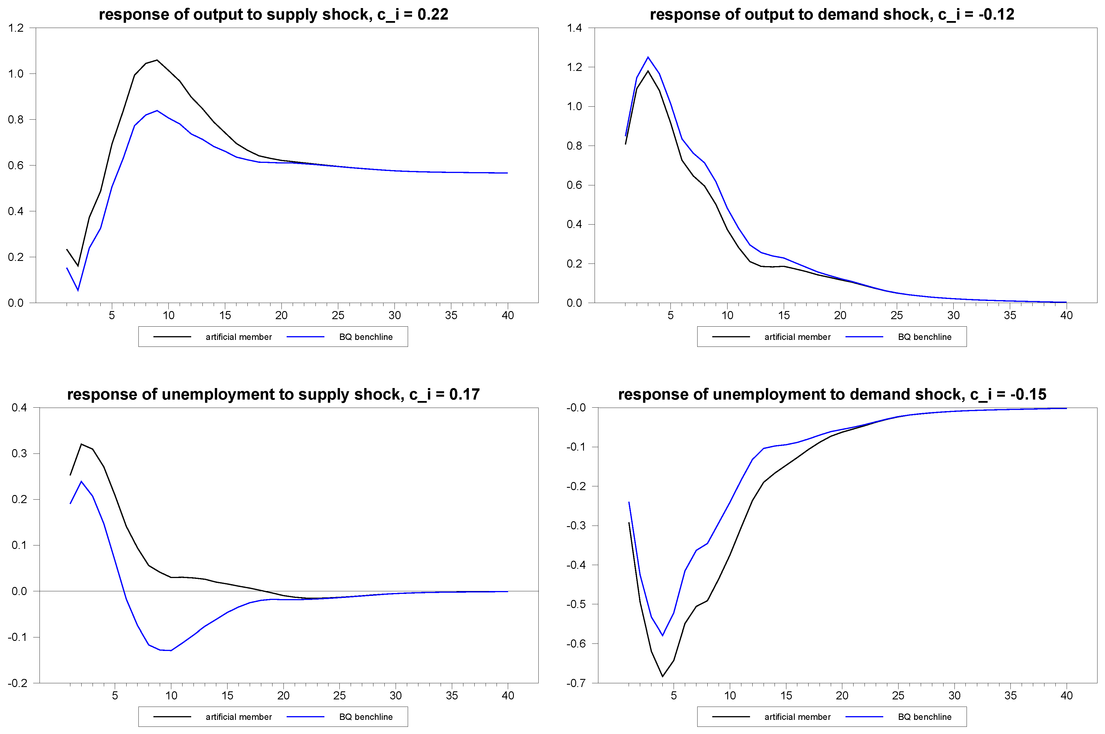
Figure 1.
Example of dynamic heterogeneity induced by exponential quadratic.

To give a sense of the manner in which the exponential quadratic function represented in Equation (12) creates heterogeneity in the dynamics, we illustrate in Figure 1 the composite responses for a typical individual member with the random values indicated in the graphics as compared to an individual member with set to , which, therefore, represents the Blanchard and Quah estimate of the response of unemployment to a supply shock in the latter case. In other words, represents the Blanchard and Quah estimates.
Notice that the two series differ considerably in the initial impacts and continue to diverge from one another, until the difference between them peaks at the eighth quarter. The heterogeneity then persists, but eventually dies out, so that the steady state restrictions are not inadvertently violated by the artificially-induced heterogeneity. When we simulate panels, we will set , so that we consider heterogeneity in the dynamic responses with the being drawn from .
Now that we have created heterogeneity in the structural dynamics, we also create heterogeneity in the loading matrices for the common versus idiosyncratic shocks, . Since, of course, the Blanchard and Quah estimates are for a single country and do not have information about these, for the purposes of our Monte Carlo simulations, we arbitrarily decompose the Blanchard and Quah composite structural shocks into hypothetical common and idiosyncratic structural shocks by setting and . We then draw the values for from uniform distributions, such that and . As discussed in Section 2, is also equivalent to the correlation between the composite and common structural shocks for each member, i, and, as such, must be bounded between 0.0 and 1.0. Accordingly, the choice of values is also bounded. Toward this end, in our simulations that follow, we set and , so that is drawn from and is drawn from . Similar to our treatment of the parameter matrix , we recenter the values after sampling, so that the values we assign to the Blanchard and Quah responses become the true mean responses of the panel DGP. Correspondingly, the common and idiosyncratic responses have an added layer of heterogeneity beyond the values, due to the heterogeneity in the loadings.
Before proceeding to the estimation stage, it is worth noting how Blanchard and Quah’s identification scheme translates intuitively into a heterogeneous panel context if we were to imagine the members of the panel as individual national economies. By using the same recursive long run structure for both the common and idiosyncratic steady state responses, we are implying that an aggregate demand shock is neutral on output regardless of whether its origin is local or global and has a similar response pattern up to a factor associated with the loading vector. While this is not necessary, it is convenient because it implies that a similar single country VAR analysis would be effectively uncovering the responses to composite aggregate supply and demand shocks. By contrast, if we apply different identification schemes for the responses to the common versus idiosyncratic responses, the implication would be that an analogous single country structural VAR analysis would have incorrectly identified the composite aggregate supply and demand shocks. The heterogeneous dynamics that are accounted for in our panel approach reflect the presumption that the particular pattern of the response to both the common and idiosyncratic shocks is potentially very different among different countries, and in this sense, the heterogeneity in the dynamic responses are virtually unconstrained with the exception of the identifying restriction itself. Specifically, the heterogeneous responses are a consequence of two features: firstly, the fact that the underlying dynamics are inherently different among the members; and secondly, the loading vectors that decompose the composite shocks and responses are also heterogeneous.
In practice, long run identification schemes that employ the restrictions associated with Equation (7) also require that the individual data follow unit root processes, even after time effects have been extracted. Furthermore, in this particular identification, the accumulated values of unemployment and the non-accumulated values of output should not cointegrate. Standard panel unit root and panel cointegration tests that allow for dynamic heterogeneity can be used to confirm this when they are unable to reject the null of a unit root for all members and the null of no cointegration for all members. Of course, one also needs to guard against the possibility that an inability to reject a unit root for all members of the panel is not due to the presence of a small number of unit roots shared among the different members of the panel in the form of cross member cointegrating relationships. For this, tests for the rank in univariate panels, as developed in Pedroni, Vogelsang, Wagner and Westerlund [13], can be used, which are robust to unknown and unspecified forms of cross-sectional dependence. Identification schemes that only employ restrictions associated with Equations (5) or (6) do not require these unit root properties.
For the long run identification scheme, once the unit root, cointegration and rank properties have been examined in the panel, the next step is to estimate the composite reduced form VAR for each member of the panel. For this, one must choose a suitable lag truncation, which will likely differ across members. In our simulation analysis, we found that the general to specific method of testing down for the significance of the highest order lag performed best among the commonly used methods for choosing lag truncation, and so, our reported results use this method. We adjusted the starting value for this selection method according to the time series dimension of the panel, so that for lengths , we tested down from two lags, for , we tested down from four lags, for , we tested down from eight lags, and for , we tested down from twelve lags.
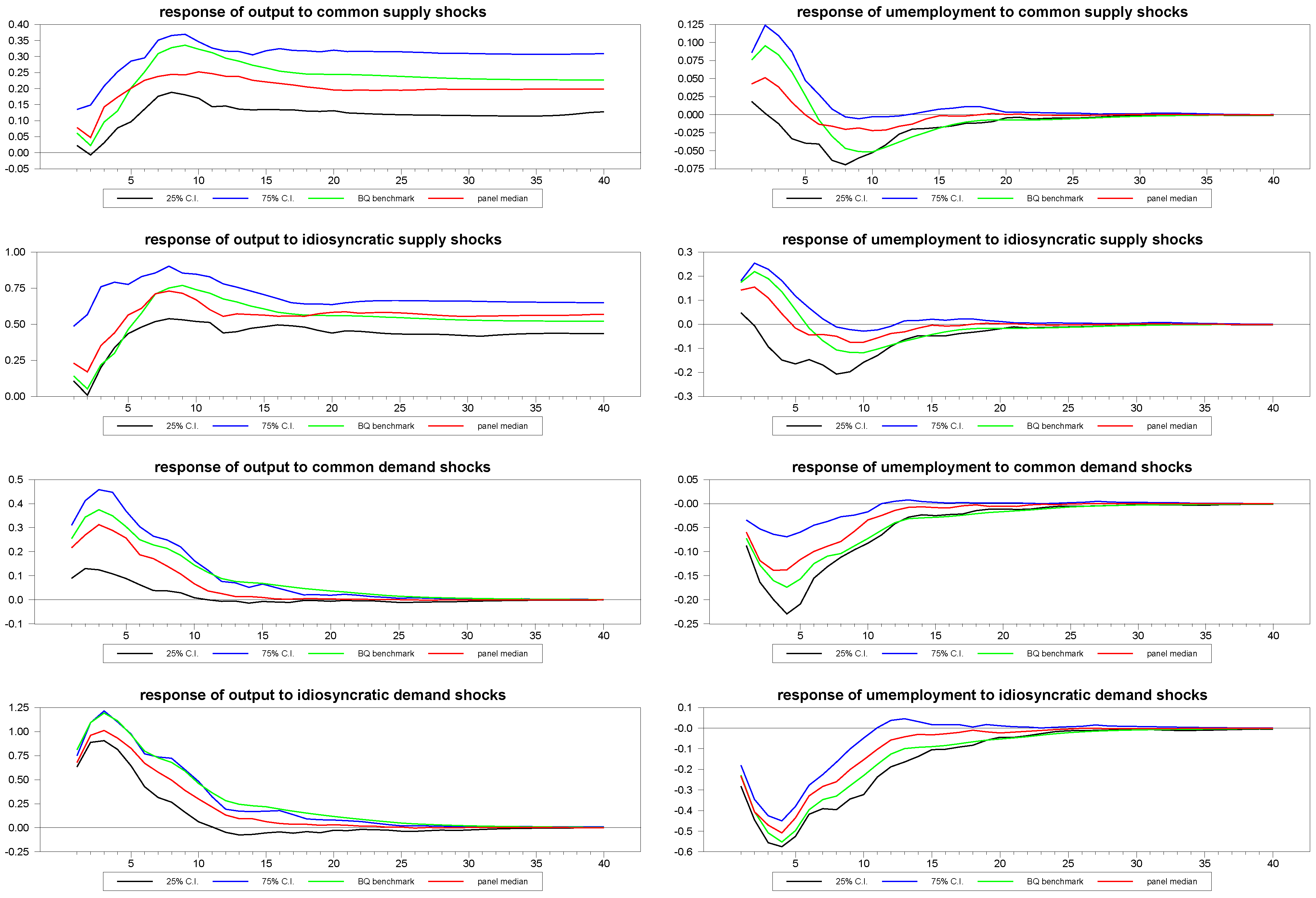
In our first illustration, as reported in Figure 2, we give a sense of what the typical median responses and associated confidence intervals for the common and idiosyncratic shocks look like for a fairly sizable panel with , . The true DGP for the mean of the sample, which is equivalent to the Blanchard and Quah estimates, is also depicted in the diagrams. As we can see, the panel SVAR does fairly well in uncovering the true underlying structural dynamics.
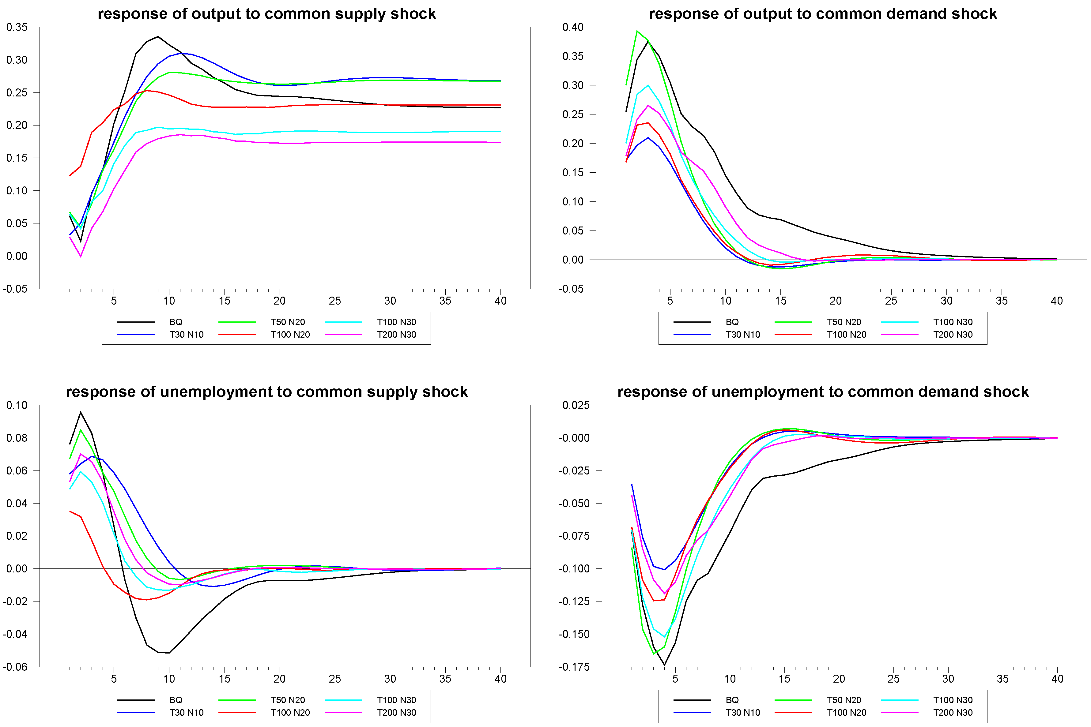
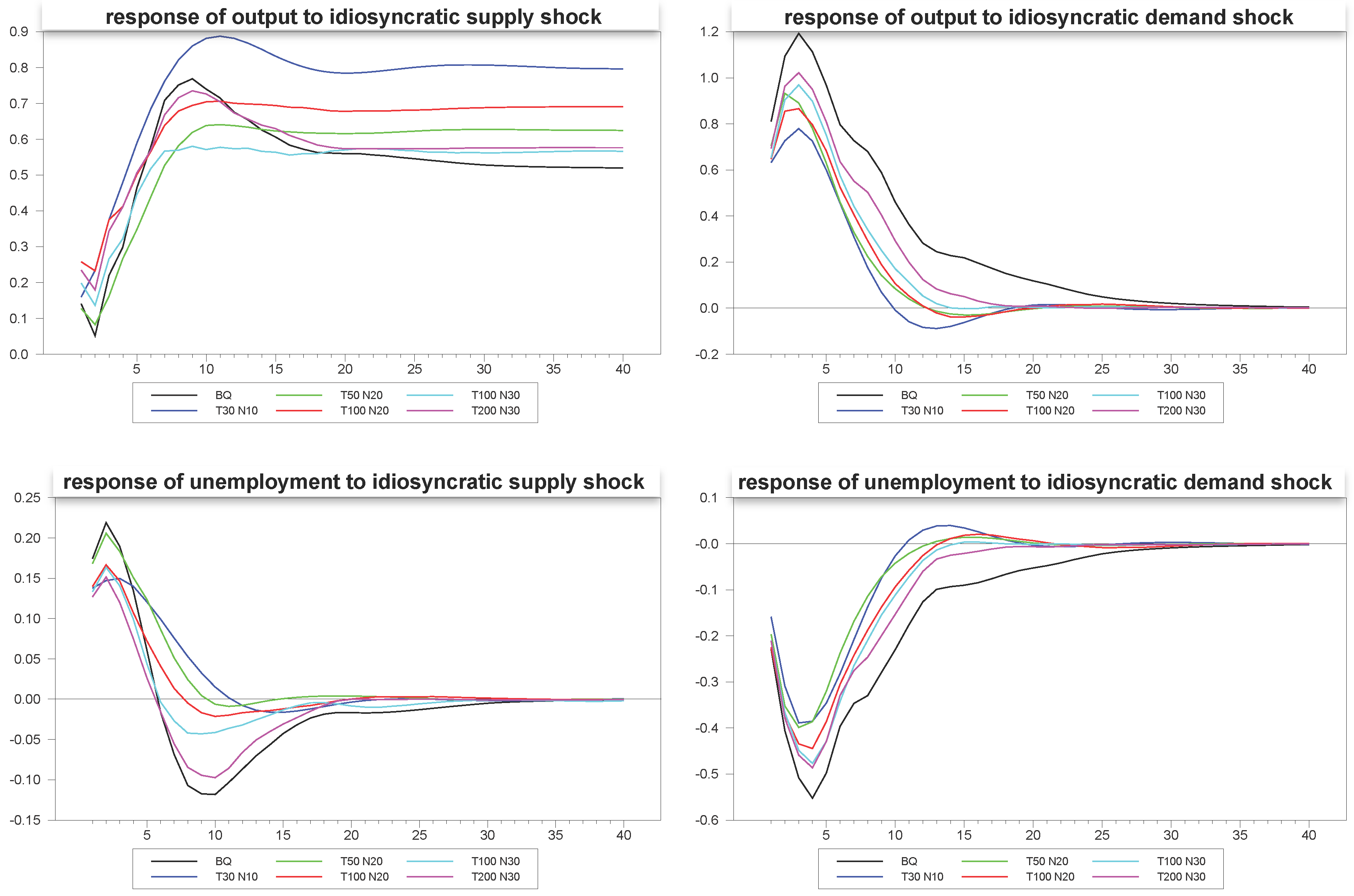
However, the dimensions , are fairly generous, and in many applications, we imagine far smaller panels. In the next set of Figure 3 through Figure 5 we depict an example of the mean estimates for panels with varying dimensions, with the true mean of the sample again depicted for comparison. As is to be expected, the larger the panel, the closer the median comes to estimating the true mean of the DGP despite the considerable heterogeneity in the underlying dynamics. What is remarkable is that even the fairly small panels with and do fairly well, not only for the responses to the composite shocks, but also in response to the common and idiosyncratic shocks, for which the technique must struggle with the additional layer of heterogeneity induced by the member-specific variations in the loading matrices for these.
Figure 2.
Panel estimates with confidence intervals, T = 200, N = 30.
Next, we investigate the small sample performance of another important feature of this panel method, which is the ability to improve inferences for individual members of the panel. As discussed in Section (2), the idea is to correlate the pattern of the sample distribution of impulse response estimates cross-sectionally with static observables as per Equation (10), and, then, use the fitted values of these along with the individual member estimates of the loading matrices to obtain fitted value estimates of the member-specific impulse response functions as described in Equation (11). For example, with the Blanchard and Quah example, one might anticipate that static measures of labor market rigidities might correlate with the response of unemployment to either aggregate supply or demand shocks across different national economies, and so forth. One might even hope to be able to use such a panel method to reliably estimate country-specific impulse responses for countries without sufficient data to estimate a time series VAR.
Figure 3.
Response estimates to composite shocks for various sample sizes.
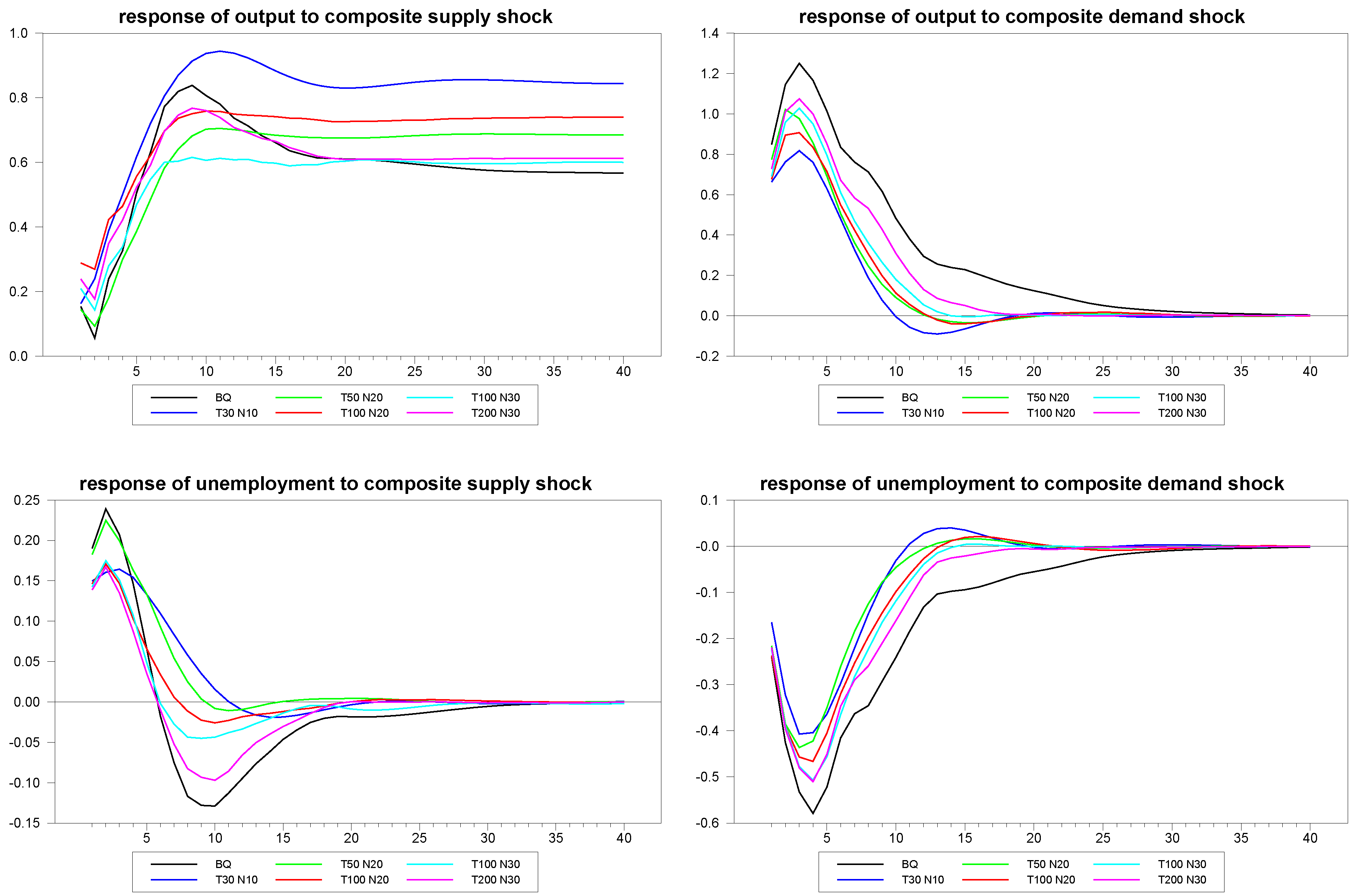
Figure 4.
Response estimates to common shocks for various sample sizes.

Figure 5.
Response estimates to idiosyncratic shocks for various sample sizes.
To simulate this, we generated an matrix of artificial static measures, , for each member, i, which was weakly correlated to the parameter values of , which were responsible for creating the heterogeneity. Keep in mind, however, that the heterogeneity in the actual structural responses, and , are then nonlinear functions of and , due to the exponential quadratic function that generate the heterogeneity in the responses as per Equations (13) and (14). Specifically, we set where is drawn from a multivariate standard normal distribution. The noise associated with is thus fairly large relative to the variation in , and accordingly, this implies a very weak correlation between the elements of and , as we might expect in many applications. For example, in a typical simulation run, the sample correlation between the four elements of and were quite low, at 0.178, 0.063, −0.068 and 0.048, respectively.
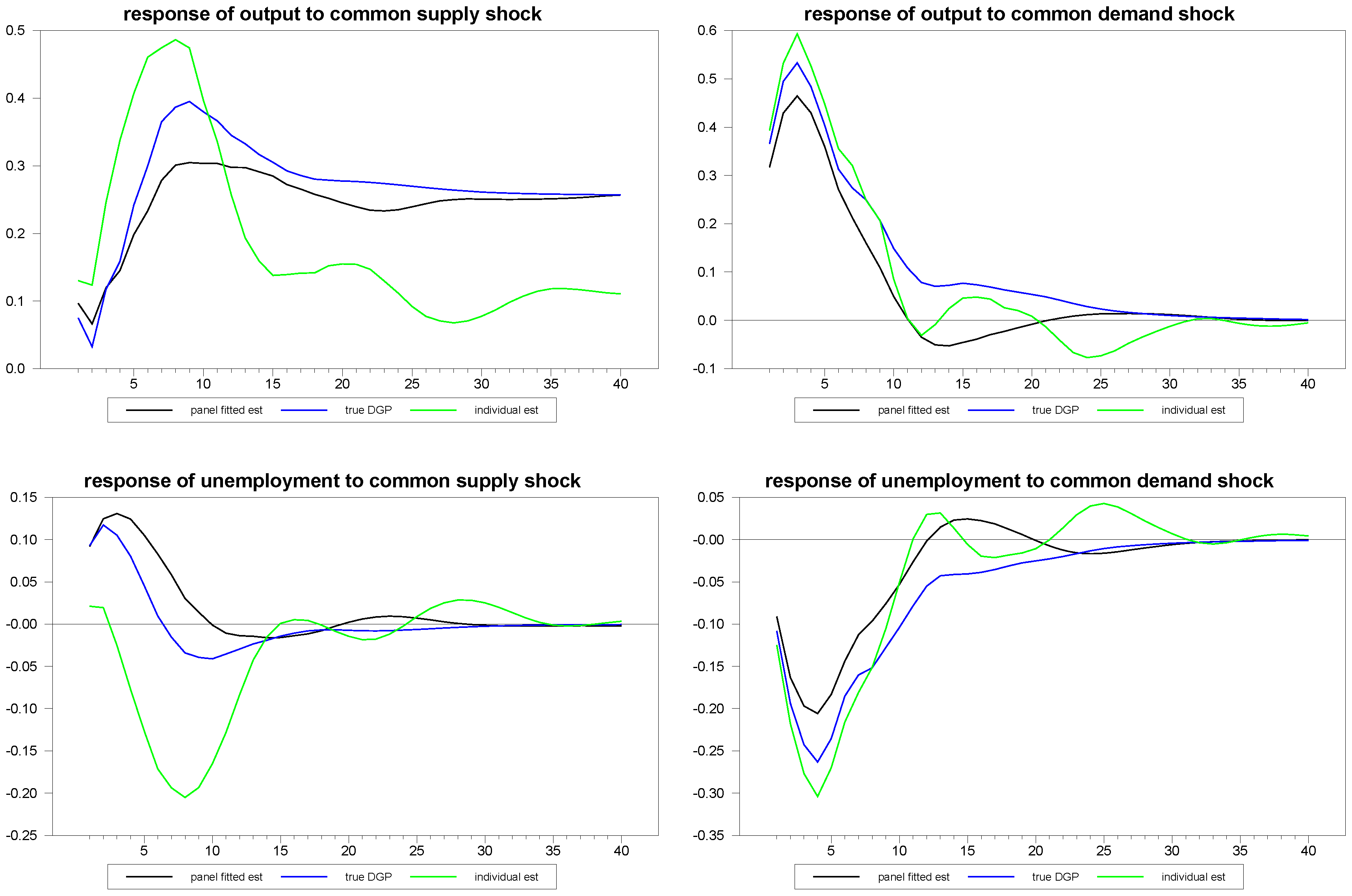
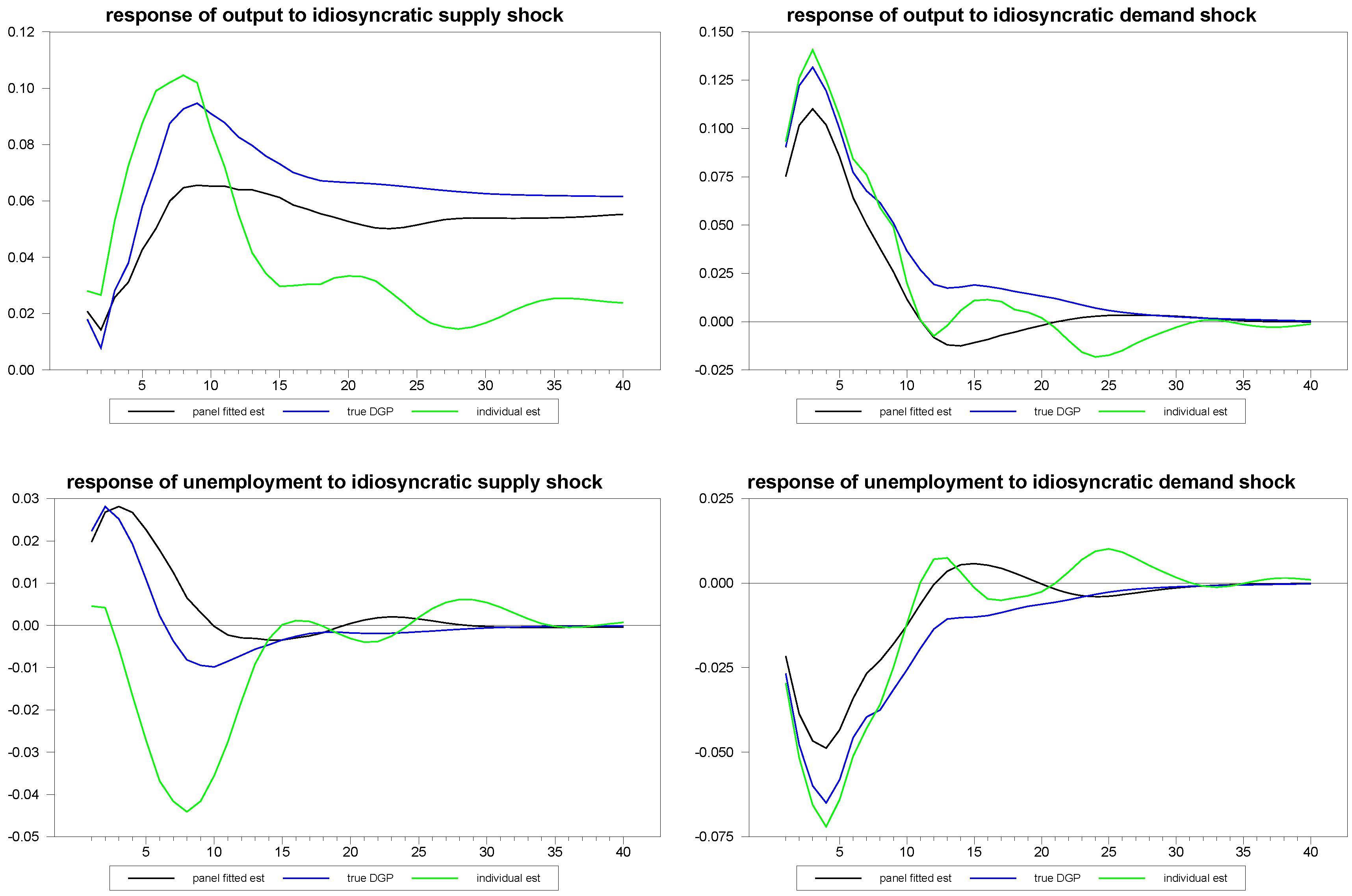
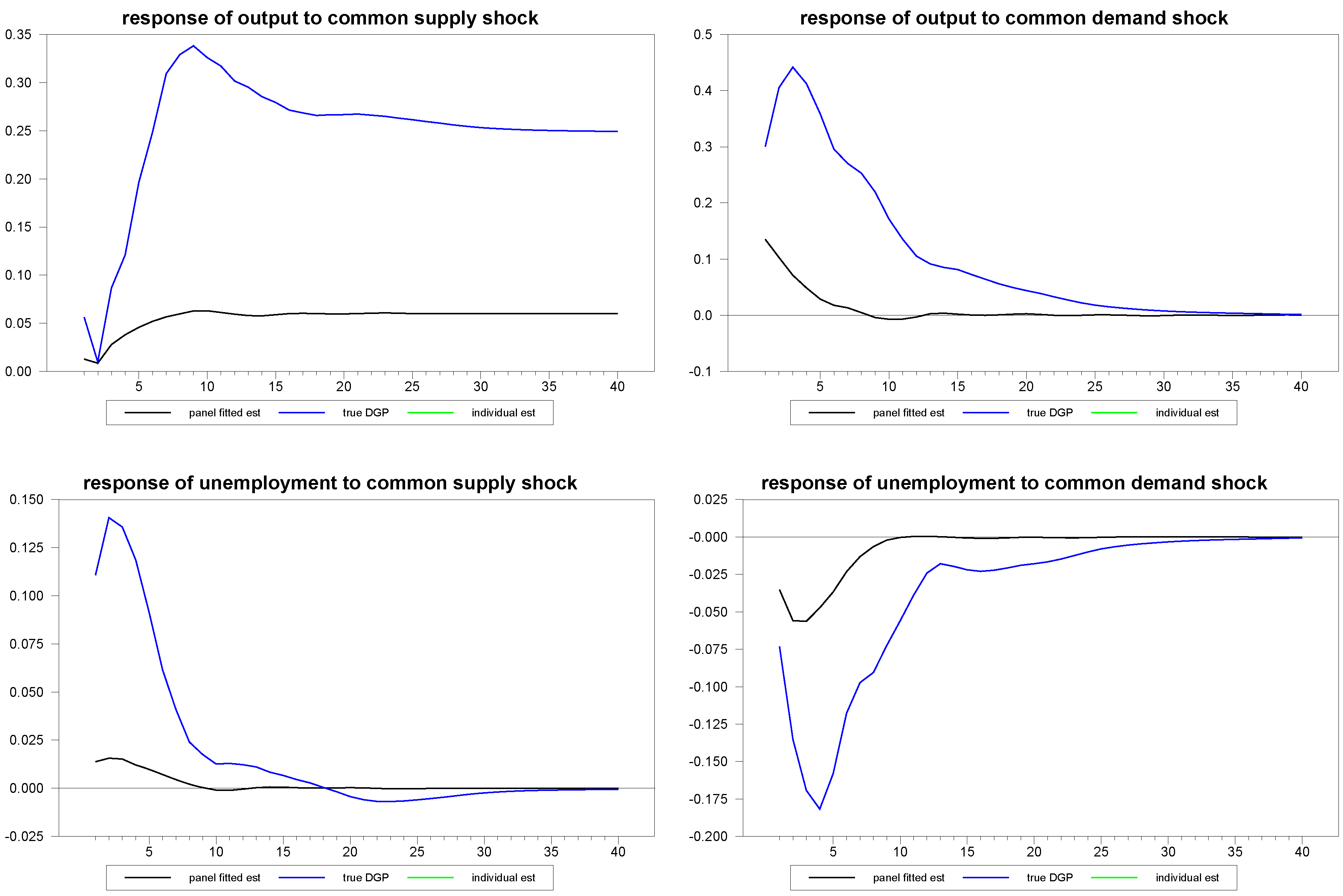
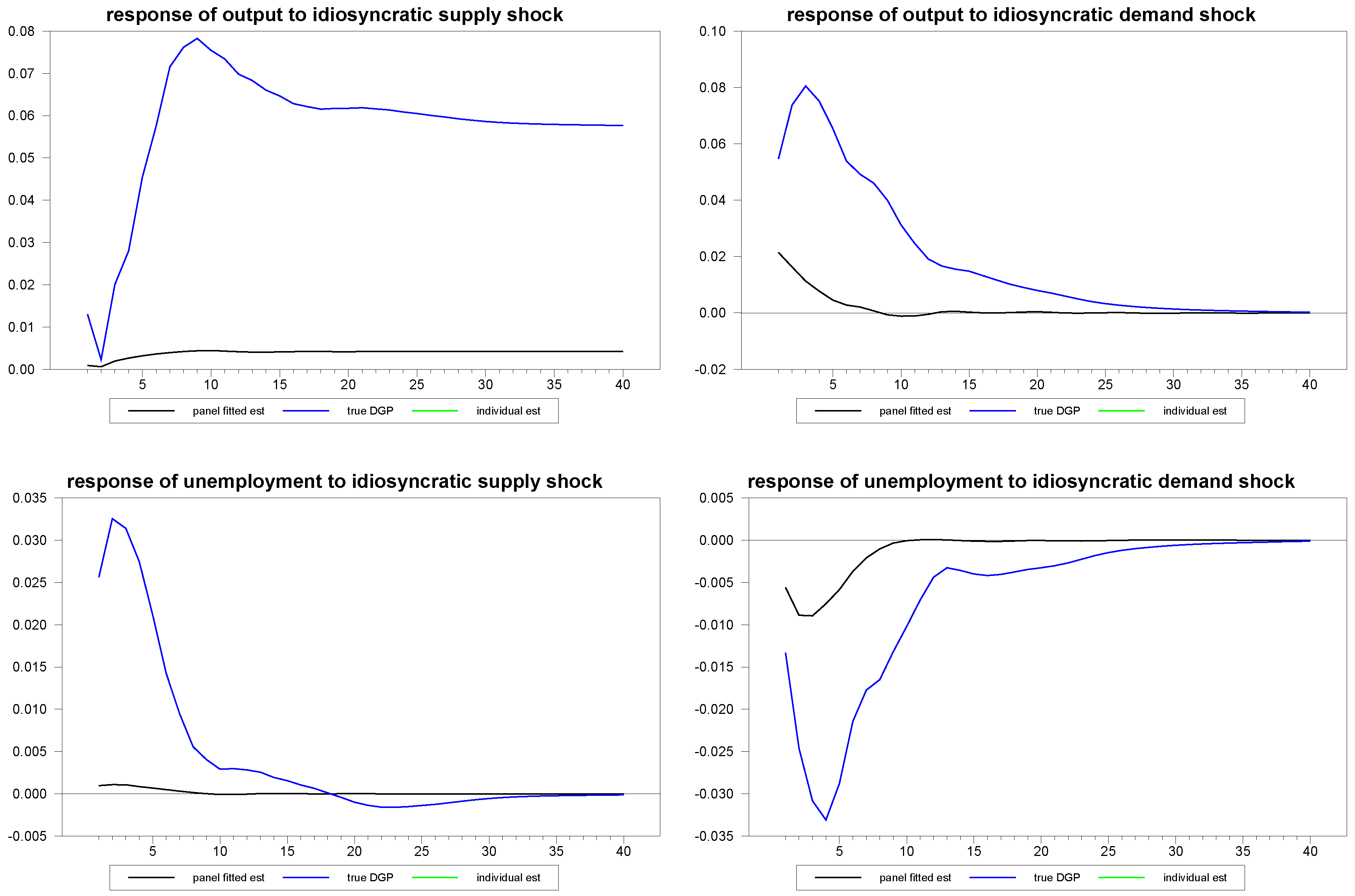
First, we examine the performance of this approach in a panel with a moderately long time series, so that we can compare such a panel fitted individual member estimate with the performance of the pure time series estimate. For this, we generated an artificial panel of dimensions , and had the random number generator randomly choose a member of the panel to represent the individual member to be estimated. We then estimated this member’s structural impulse responses using both the fitted panel approach and using a pure time series estimate without the benefit of the panel. Figure 6 shows the results for the various estimates of the responses of the first member of the panel to the composite structural shocks. The blue line represents the true simulated values of the DGP; the green line represents the individual time series estimates without the benefit of the panel, and the black line represents the panel fitted individual member estimates. Even with a series as long as , the panel approach improves the estimates substantially. In Figure 7 and Figure 8, we report similar estimates for the responses to common and idiosyncratic shocks, respectively. For the sake of comparison, we use the individual estimates for the individual time series estimates of these responses, even though, in practice, the estimation of the are only possible with the use of the panel, as is done for the panel fitted member-specific estimates.
Next, we examine the very extreme case in which the time series dimension is much too short to reliably use pure time series methods and ask whether the fitted panel method can produce a sensible estimate for the randomly chosen individual member response. To simulate this, we generated an artificial panel with dimensions and . With a time series of length , one cannot reliably estimate a structural VAR by time series methods. Yet, remarkably, the fitted panel method appears to be able to recover at least some of the features of the structural dynamics for the individual member.
Figure 6.
Panel fitted individual member response estimates to composite shocks for N=30, T=100.
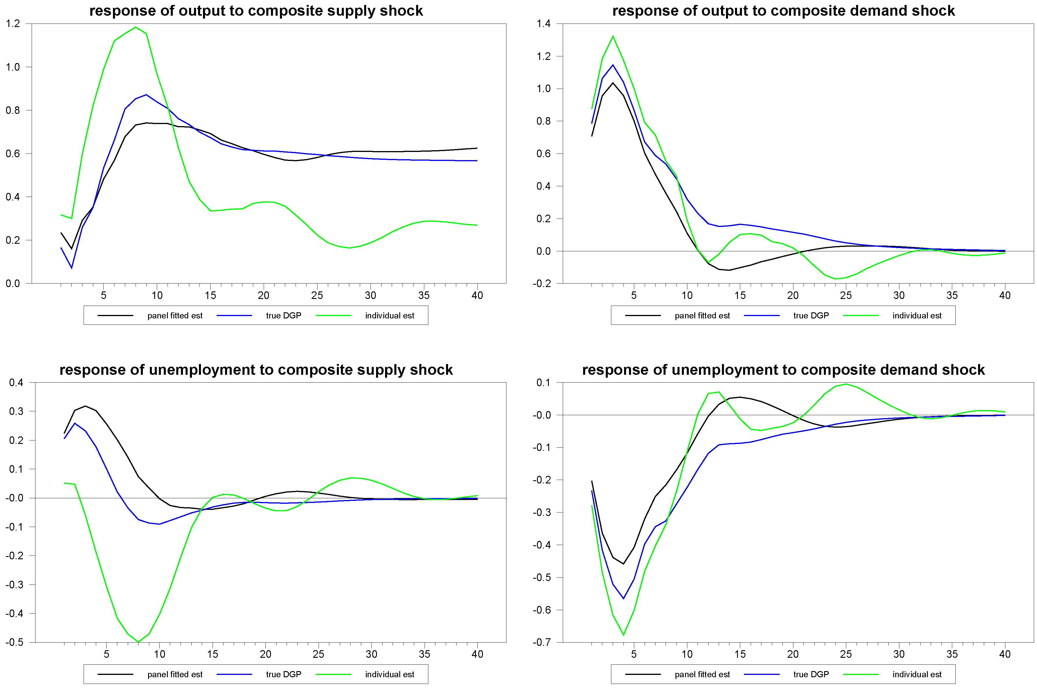
Figure 7.
Panel fitted individual member response estimates to common shocks for N=30, T=100.

Figure 8.
Panel fitted individual member response estimates to idiosyncratic shocks for N=30, T=100.
Figure 8.
Panel fitted individual member response estimates to idiosyncratic shocks for N=30, T=100.

We noticed something interesting in the previous simulations, which became even more pronounced as the T dimension became shorter. Even though the DGP ensures that is stationary, every once in a while, the estimated values of the VAR coefficients will be outside the range of stationarity, with the result that the accumulated impulse responses diverge and, in effect, become extreme outliers. By using median estimators rather than mean estimators, the effect of a few divergent impulse responses is negligible. However, as the T becomes very short and individual estimates become poorer, the number of divergent impulse responses increases, to the point of having a small, but noticeable, effect even on the median estimates. One simple remedy was to toss any of the divergent responses, at which point the mean estimator can be used. This can be automated very simply by tossing any response that does not return to within some tolerance of zero in the differences by the 40th response period. For our tolerance level, we used 0.01. However, the improvement was not substantial enough to warrant recommending this over the simpler method of using the median. However, in cases where panel fitted individual member responses are estimated rather than panel averages, the issue becomes more salient. Even in the cases when we estimate panel fitted values, the trimming is unnecessary. However, for the case when we estimate panel fitted values for panels with very short T, the improvement was enough to warrant using this approach, which was, therefore, employed in generating Figure 9 through Figure 11.
Figure 9.
Panel fitted individual member response estimates to composite shocks for N=50, T=12.
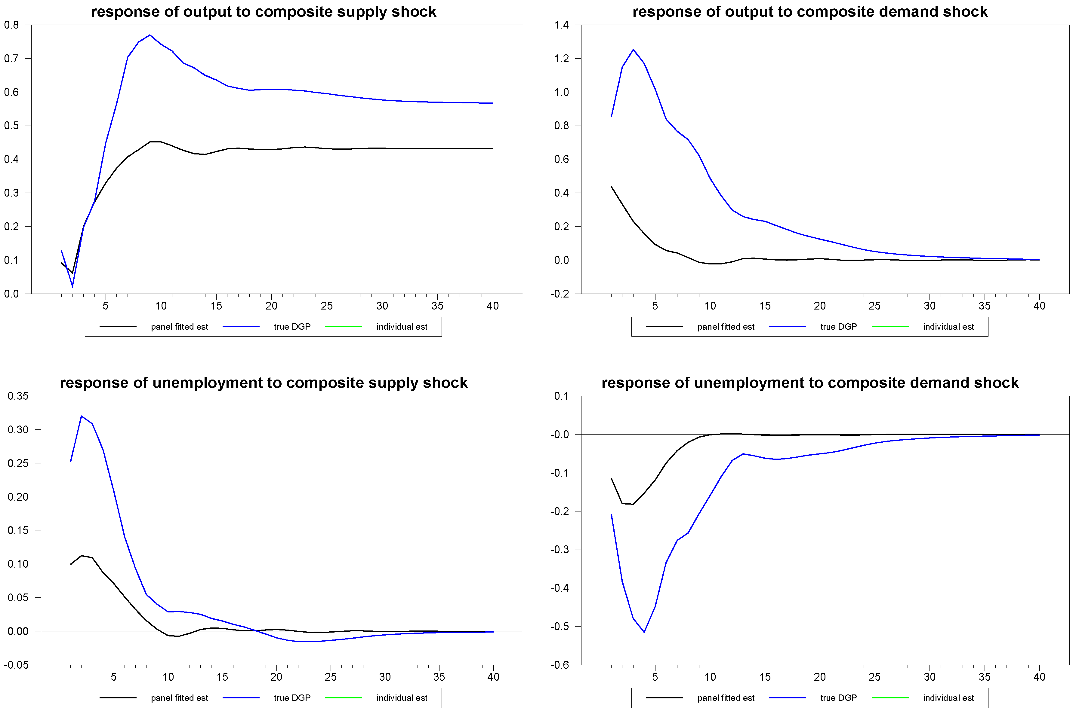
Figure 10.
Panel fitted individual member response estimates to common shocks for N=50, T=12.

Figure 11.
Panel fitted individual member response estimates to idiosyncratic shocks for N=50, T=12.
Figure 11.
Panel fitted individual member response estimates to idiosyncratic shocks for N=50, T=12.

This observation is also consistent with an intuition as to why the method works as well as it does. The idea is that as T becomes very short, for many of the individual members, the time series estimates become unreliable, with many becoming divergent. However, many are also non-divergent, and while they do not produce accurate estimates, they do contain a faint signal regarding the true dynamic structure. By correlating the signal cross-sectionally with a static observable, the method appears to able to extract this signal. By using the fitted cross-sectional regression estimates, we are then able to trace out an estimate of the true structural dynamic for the individual member, even when the time series dimension, , is very short, as illustrated in Figure 9 through Figure 11.
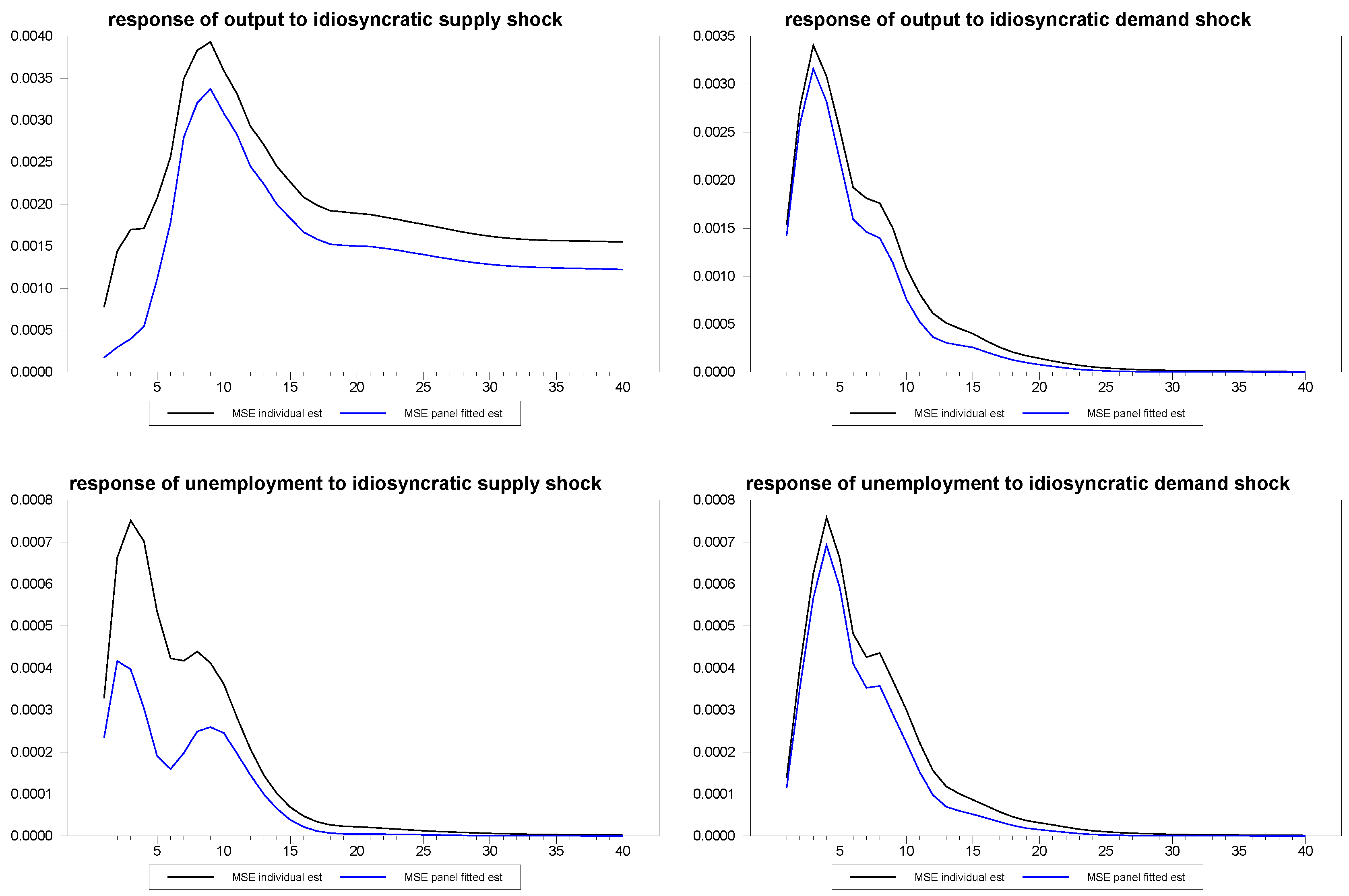
To more formally depict the improvement that the panel method brings to individual member estimates, we compared the mean squared error, MSE, of the estimates. Specifically, we were interested in comparing the MSE for a scenario in which the individual time series estimates were viable, and compare these to the panel fitted individual member estimates. Toward this end, we generated 2,000 artificial panels with dimensions and . For each panel, we drew new values for the parameters, , and , subject to the same i.i.d. distributions for each draw, so that the specific sample draws for these values would have less influence on the results. Again, we allowed the random number generator to arbitrarily chose the member of the panel. We did this once, keeping the chosen member of the panel fixed for all 2,000 artificial panels and, then, we repeated the experiment allowing the randomly chosen member of the panel to vary with each of the 2,000 artificial panels and found similar results as expected. The results for the fixed member case are depicted in Figure 12 through Figure 14. As can be seen in the figures, the panel fitted approach appears to substantially outperform the individual time series estimates at all time horizons.
Figure 12.
Mean squared error (MSE) for panel fitted individual member response estimates to composite shocks for N=30, T=100.
Figure 12.
Mean squared error (MSE) for panel fitted individual member response estimates to composite shocks for N=30, T=100.
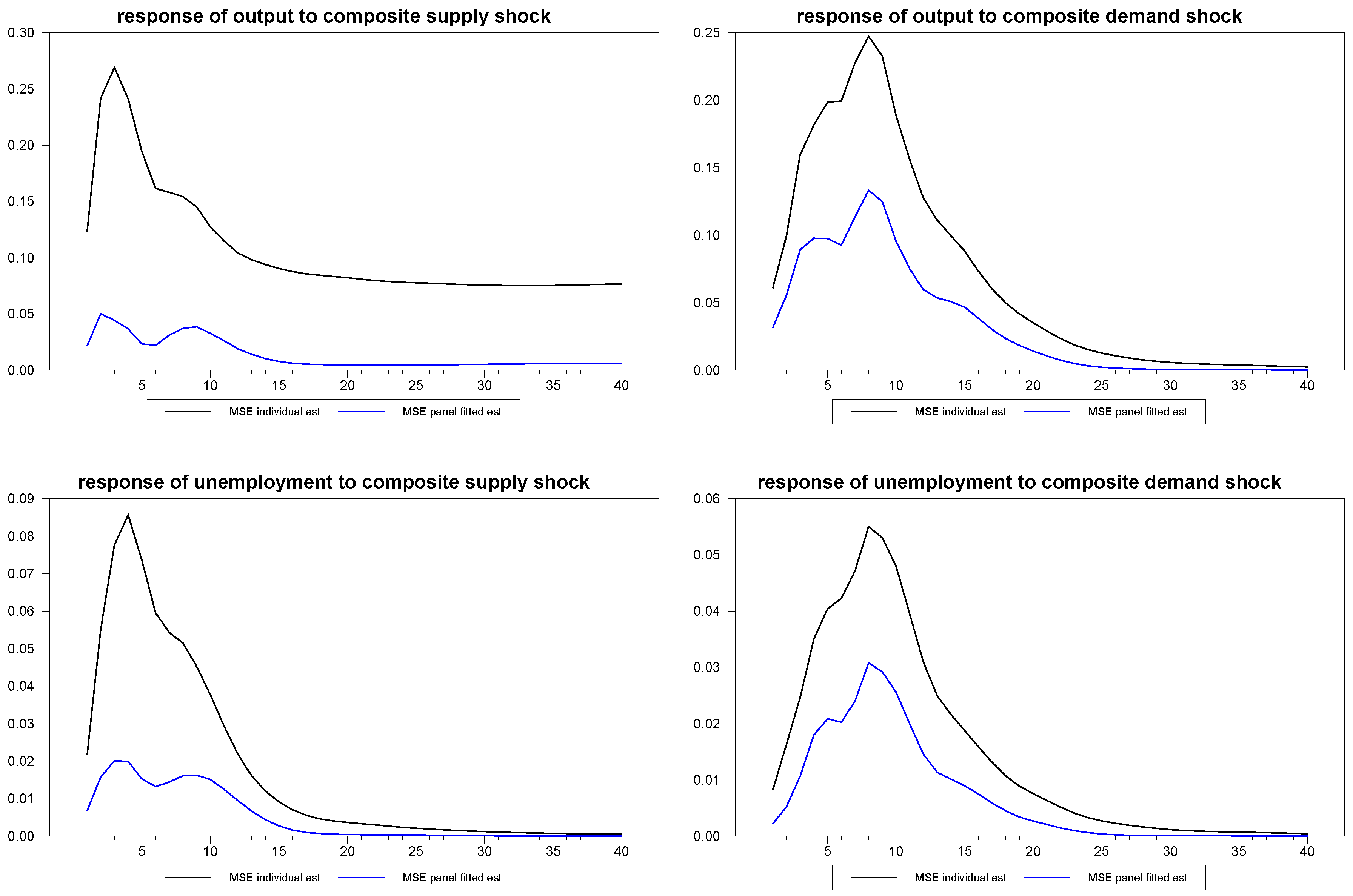
Figure 13.
MSE for panel fitted individual member response estimates to common shocks for N=30, T=100.
Figure 13.
MSE for panel fitted individual member response estimates to common shocks for N=30, T=100.
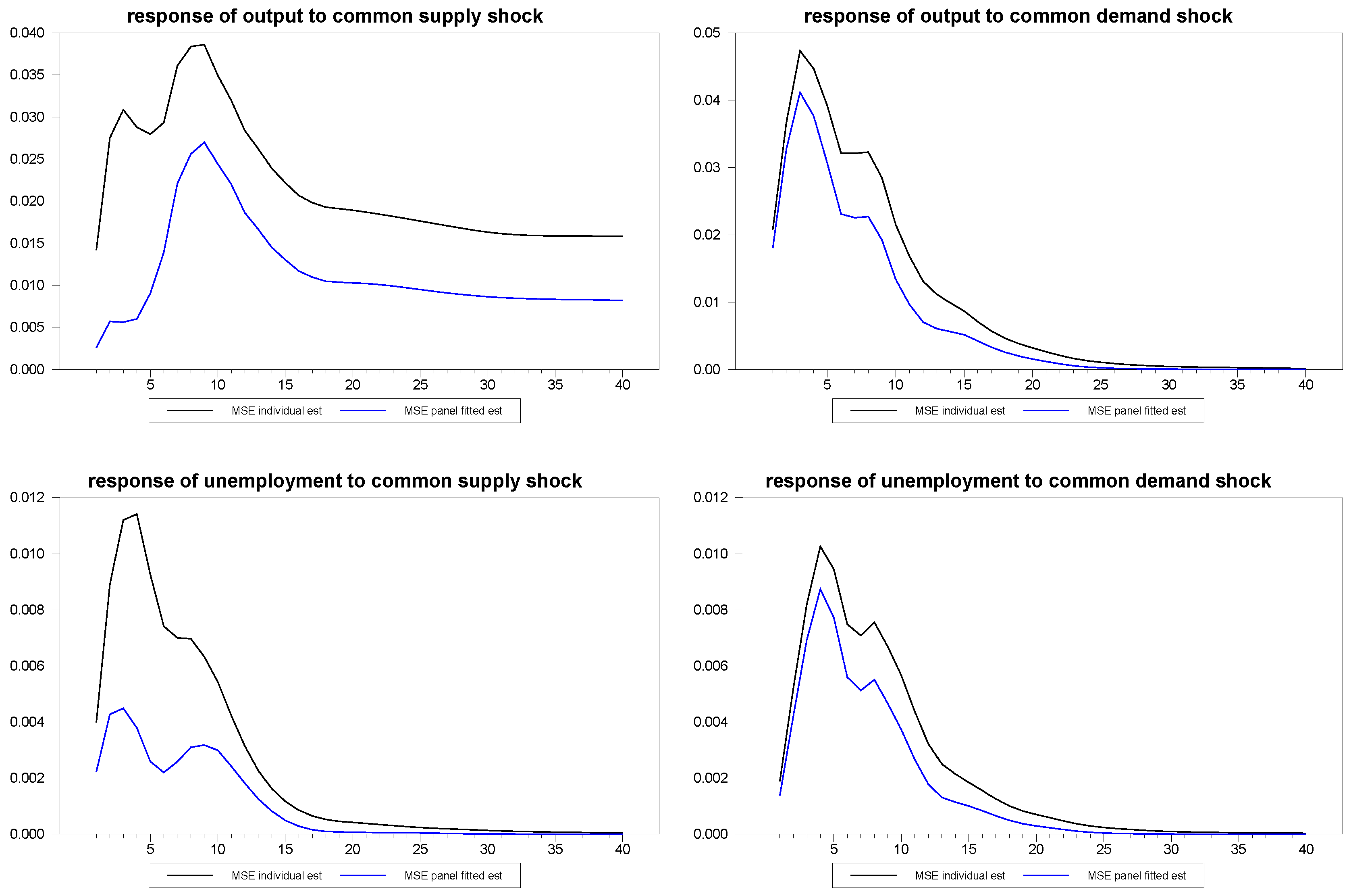
Figure 14.
MSE for panel fittend individual member response estimates to idiosyncratic shocks for N=30, T=100.
Figure 14.
MSE for panel fittend individual member response estimates to idiosyncratic shocks for N=30, T=100.
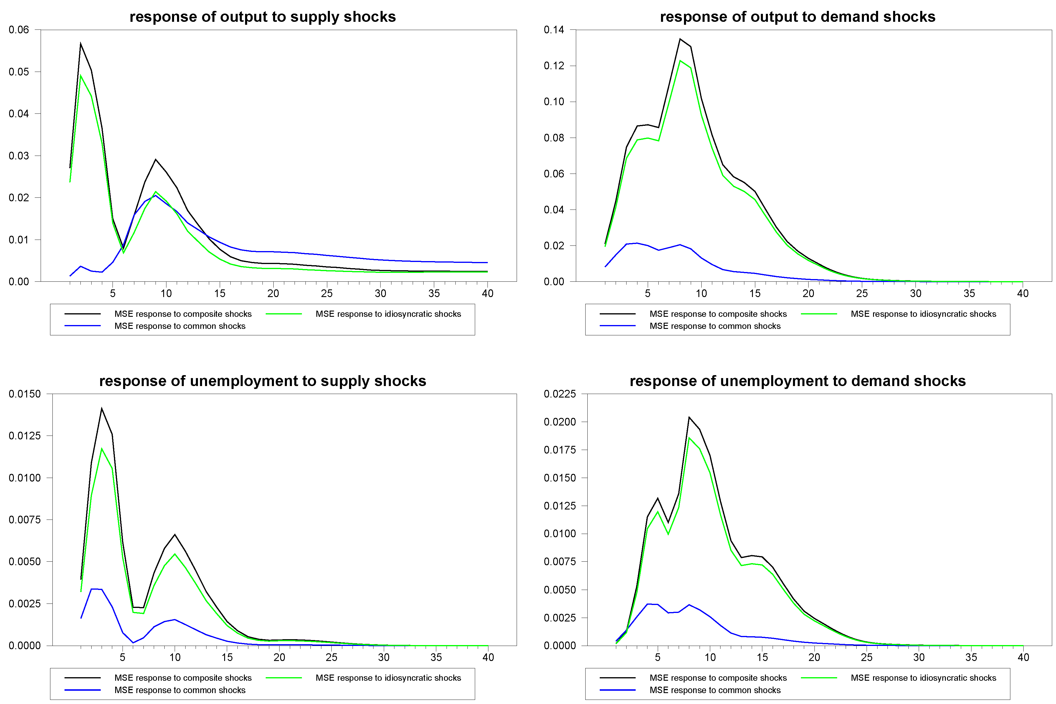
Finally, we produced similar MSE estimates for the panel median estimator, as depicted in Figure 15. It is interesting to note that the MSE for the response to the common shock is consistently lower than that of the responses to the composite and idiosyncratic shocks. This makes sense, because the signal from the common shock is contained in the data for all panel members, while the signal for response to the idiosyncratic shock, and therefore, also, a portion of the response to the composite shock, is contained only in the corresponding individual member.
Figure 15.
MSE for panel median response estimates for N=30, T=100.
Interestingly, the results on the panel fitted approach suggest that the panel median estimates could be further improved by fitting all individual members of the panel prior to computing the group median, which we leave to future research to explore. Similarly, if cross-sectional correlates for the loading vectors are used, this may further improve the small sample performance. In applications, a natural correlate to consider would be the inverse of the size of the member as a share of the panel.
4. Concluding Remarks
We have proposed here a method to study structural VARs in panels. The method decomposes the shocks and impulse responses into member-specific idiosyncratic structural shocks and common structural shocks that drive the cross-sectional dependence among members. The structural-based approach makes these decompositions straightforward and transparent. It also allows for heterogeneous member-specific dynamics in response to both sets of shocks. The technique can be used to infer dynamics about features of the sample distribution among members, such as the median response, and it can also be used to improve estimates for individual member responses. This suggests that the methods are well suited for a number of panel data types that are expected to have heterogeneous dynamics and cross-sectional dependencies arising from responses to commonly shared structural shocks. A few examples of empirical applications based on the panel SVAR methodology developed in earlier drafts of this paper include, among others, Mishra et al. [10], Pedroni and Sheppard [12] and Montiel and Pedroni [11].
The approach appears to hold promise for empirical research, and there are several further avenues of exploration that have been touched upon in this analysis and warrant further investigation. For example, to reiterate a few of these, it might be worthwhile to explore whether bootstrapping might further improve the performance of the approach. One attractive feature of the approach presented in this paper is that a bootstrap is not necessary if one is simply interested in presenting confidence intervals for the cross member distribution of dynamic responses, as we have done. However, there is nothing that prevents one from also applying a conventional bootstrap to each member of the panel, as would be done in a time series-based VAR, and, in turn, using these to construct confidence intervals for the median responses. If one is concerned with control for any remaining sources of cross-sectional dependence beyond the primary source arising from the member-specific responses to common shocks, a block bootstrap that samples across members for each block of time may prove to be fruitful.
Other interesting avenues that we are exploring include extensions of the method of fitting the members of the panel to cross-sectional correlates. As discussed in this paper, one possibility may be to use the fitted panel approach on all members of the panel prior to estimating sample properties, such as the group median. As also discussed, it will be interesting to explore the use of cross-sectional correlates that might improve the estimates of the member-specific loading matrices that decompose the shocks and responses into common versus idiosyncratic components. If this is applied to a multi-country panel framework, it would also imply that it might be possible to obtain reasonable estimates for the structural dynamics for countries that do not themselves have reliable time series data, not only for the responses to composite shocks, which can already be done based on the method described in this paper, but also for the responses to common and idiosyncratic responses that require estimates of the loading matrices.
Finally, it will be interesting to compare the small sample performance of this panel SVAR approach under different possible types of identification schemes, as described in Section 2 of the paper. It will also be useful to explore the small sample properties of other commonly used tools in SVAR analysis, such as the associated variance decompositions and historical decompositions. VARs with known shock dates, such as is typical for time series-based event analysis studies, are also possibilities that are being explored as relatively straightforward special cases of the techniques developed in this paper.
The use of time effects to account for common factors has shown success in other areas of panel econometrics, such as, for example, Pesaran [14], and, as we have demonstrated, appears to be a fruitful avenue for capturing common shocks in structural-based approaches to VARs in panels, as well. Recent generalizations of the dynamic factor model approach, such as, for example, the recent work of Forni and Lippi [9], may also hold promise for future directions in which panel SVARs can be further generalized.
Acknowledgements
We thank three anonymous referees for their helpful and constructive comments, and Jean-Pierre Urbain and others for helpful comments. We also thank the following conference and seminar participants for feedback on earlier versions: American Economic Association Meetings, Bank of Italy, Coimbra University, Javeriana University, International Monetary Fund, Central Bank of Peru, University of Barcelona Conference on Regional and Urban Economics, Conference on Monetary Policy in Small Open Economies and the National Bank of Georgia.
Conflicts of Interest
The author declares no conflict of interest.
References
- M. Arellano, and S. Bond. “Some Tests of Specification for Panel Data: Monte Carlo Evidence and an Application to Employment Equations.” Rev. Econ. Stud. 58 (1991): 277–97. [Google Scholar]
- B. Bernanke. “Alternative Explanations of the Money-Income Correlation.” Carn. Roch. Conf. Serie. 25 (1986): 49–99. [Google Scholar] [CrossRef]
- O. Blanchard, and D. Quah. “The Dynamic Effects of Aggregate Demand and Supply Disturbances.” Am. Econ. Rev. 79 (1989): 655–73. [Google Scholar]
- O. Blanchard, and M. Watson. “Are all Business Cycles Alike? ” In The American Business Cycle. Edited by R. Gordon. Chicago, USA: University of Chicago Press, 1986, pp. 123–56. [Google Scholar]
- F. Canova, and M. Ciccarelli. “Forecasting and Turning Point Prediction in a Bayesian panel VAR Model.” J. Econom., 327 (2004): 327–59. [Google Scholar] [CrossRef]
- F. Canova, and M. Ciccarelli. “Estimating Multicountry VAR Models.” Int. Econ. Rev. (Philadelphia) 50 (2009): 929–59. [Google Scholar] [CrossRef]
- R. Clarida, and J. Gali. “Sources of Real Exchange Eate Fluctuations: How Important are Nominal Shocks? ” Carn. Roch. Conf. Serie. 41 (1994): 1–56. [Google Scholar]
- D. Holz-Eakin, W. Newey, and H. Rosen. “Estimating Vector Autogressions with Panel Data.” Econometrica 56 (1988): 1371–95. [Google Scholar] [CrossRef]
- M. Forni, and M. M. Lippi. “The General Dynamic Factor Model: one-sided representation results.” J. Econom. 163 (2011): 23–28. [Google Scholar] [CrossRef]
- P. Mishra, P. Montiel, P. Pedroni, and A. Spilimbergo. “Monetary Policy and Bank Lending Rates in Low Income Countries: Heterogeneous Panel Estimates.” Working Paper. Washington, DC, USA: International Monetary Fund, 2012. [Google Scholar]
- P. Montiel, and P. Pedroni. “Financial integration in LICs: Empirical Measurement and Consequences for Monetary Policy.” Working Paper. Williamstown, MA, USA: Williams College, 2013. [Google Scholar]
- P. Pedroni, and S. S. Sheppard. “The Contribution of Housing Markets to the Great Recession.” Williamstown, MA, USA: Working Paper, Williams College, 2010. [Google Scholar]
- P. Pedroni, T. Vogelsang, M. Wagner, and J. Westerlund. “Nonparametric Rank Tests for Non-Stationary Panels.” Economics Series Working Paper No. 270; Vienna, Austria: Institute for Advanced Studies, 2012. [Google Scholar]
- M.H. Pesaran. “Estimation and Inference in Large Heterogenous Panels with Multifactor Error Structure.” Econometrica 74 (2006): 967–1012. [Google Scholar] [CrossRef]
- M. H. Pesaran, T. Schuermann, and S. Weiner. “Modeling Regional Interdependencies Using a Global Error-Correcting Macroeconometric Model.” J. Bus. Econ. Stat., 22 (2004): 129–62. [Google Scholar] [CrossRef]
- M. H. Pesaran, and R.P. Smith. “(1995). Estimating Long-Run Relationships from Dynamic Heterogeneous Panels.” J. Econom. 68 (1995): 79–113. [Google Scholar] [CrossRef]
- C. Sims. “Are Forecasting Models Usable for Policy Analysis? ” Fed. Reserve Bank Minneapolis Quart. Rev. 10 (1986): 2–16. [Google Scholar]
- Available online at: www.estima.com (accessed on 30 May 2013).
- 1.A copy of the computer code designed to implement the techniques developed in this paper is available upon request from the author.
- 2.In principle, the dimensionality for the vector of common shocks may be smaller than that of the idiosyncratic shocks, which can be implemented by setting for some composite shocks.)
- 3.A referee raised the interesting point that since for an unbalanced panel, is time varying, depending on one’s interpretation, might also be taken to be time varying. To avoid complications associated with this, we prefer to consider that over the full time span of the panel, for a given sample of total members, the DGP for has constant (non-time varying) moving average coefficients. In this context, the fact that is time varying for an unbalanced panel simply reflects the idea that we have a different number, , of sample realizations of the total number, N, of members for different time periods, such that .
- 4.An interesting implication is that if the restrictions were assumed to differ, it would imply that a conventional time series SVAR analysis without the benefit of the panel structure would likely incorrectly identify the various composite shocks.
- 5.We obtained the estimates using the replication code "bqexample.rpf" available for download from www.estima.com [18].
© 2013 by the authors; licensee MDPI, Basel, Switzerland. This article is an open access article distributed under the terms and conditions of the Creative Commons Attribution license (http://creativecommons.org/licenses/by/3.0/).
Share and Cite
MDPI and ACS Style
Pedroni, P. Structural Panel VARs. Econometrics 2013, 1, 180-206. https://doi.org/10.3390/econometrics1020180
AMA Style
Pedroni P. Structural Panel VARs. Econometrics. 2013; 1(2):180-206. https://doi.org/10.3390/econometrics1020180
Chicago/Turabian StylePedroni, Peter. 2013. "Structural Panel VARs" Econometrics 1, no. 2: 180-206. https://doi.org/10.3390/econometrics1020180