1. Introduction
The use of brand choice models has become standard practice in marketing research [
1,
2,
3,
4]. In many applications of these choice models, the random utility theory framework [
5,
6] is used to represent the choice process. An often made assumption used to be the homogeneity of households. That is, it was assumed that all households have similar tastes, where tastes also include features, such as price elasticity and promotion sensitivity. Differences in household behavior were only allowed to the extent that they could be fully explained by observable characteristics. This corresponds with so-called
observed heterogeneity. Taste is in this case explicitly modeled, for example, by including demographic variables (see, e.g., [
7]) or like [
8], who include survey data in their brand choice model to capture heterogeneity. Usually, however, such survey data are not available. Furthermore, many studies have shown that not all heterogeneity can be captured by available observed characteristics. Hence, there might be so-called
unobserved heterogeneity; see, for example, [
9,
10], among others.
There are two popular techniques to deal with unobserved heterogeneity; see [
11,
12] for a discussion. These techniques are both based on the notion that when there is unobserved heterogeneity in tastes, there is a corresponding preference distribution in the population. One approach imposes a continuous distribution of a known form to capture the heterogeneity; see, for example, [
10]. The other approach tries to approximate the unknown distribution by a discrete distribution with a fixed number of probability masses. A choice model using the latter approach is an example of a finite mixture model; see, for example [
13]. The mixture components are usually interpreted as segments of households with similar preferences.
In the above-mentioned approaches, tastes are usually assumed to be constant during the observation period for each household. This assumption is needed to identify the random heterogeneity. Additionally, the imposed unobserved heterogeneity structure has a priori no direct interpretation. For example, the interpretation of segments following from a mixture approach is usually done once the parameters have been estimated.
In the present paper, we propose a new approach. Next to a flexible specification of possible heterogeneity in tastes, we introduce unobserved heterogeneity in a brand choice model, which
a priori has a direct and meaningful interpretation. Furthermore, we allow heterogeneity to be different across purchase occasions within the same household [
14]. Households, who choose amongst brands within a specific product category, may differ in their response to marketing efforts. For example, some households will spend more time and effort while making their choice than others do. If little time and effort is invested in the decision process, it is perhaps less likely that the household will respond to marketing instruments [
15]. For example, to be able to respond to price changes, one, of course, needs to recall the previous prices of all brands. To be able to respond to advertising, one has to read the newspaper in which the advertisement is printed. It may be unrealistic to assume that all households show such a strong involvement with the product category at all purchase occasions, especially if we consider low involvement categories, such as various supermarket product categories. Hence, it is likely that households will differ in the extent to which they are responsive to marketing efforts. Within a household, there may also be differences in the responsiveness across purchase occasions, for example, due to different types of shopping trips [
14].
One reason why some households are unresponsive to marketing efforts could just be a lack of interest in marketing efforts made by brand managers. On the other hand, economic motivations may also explain varying responsiveness across households and over time. For example, search costs play an important role in the decision process of a household or an individual. As mentioned before, to be responsive to price changes, one needs to remember the prices of each option at each purchase occasion. Additionally, people usually face time constraints. It takes time for a household to compare the prices of all options at a specific shopping occasion at the time of purchase. Consider a household planning to buy many different items during the same shopping trip. There is obviously a limited amount of time available for the trip, and therefore, it may be unrealistic to assume that the household will allocate much time to each item. Following this line of thought, the more items a household purchases at a shopping trip, the less responsive this household might be to marketing efforts. Hence, the monetary value of all products purchased at a shopping trip may be inversely related to the responsiveness to marketing efforts.
As the decision process differs across households and across purchase occasions, the above implies that the observed choice of different households can unlikely be explained by the same variables. Choice behavior of responsive households can be explained by their base preferences, by marketing efforts and by their purchase history. Brand choice by unresponsive households may only be described by base preferences and purchase history. Moreover, household characteristics are rarely seen to significantly contribute to explaining brand choice, but these might be especially informative for the type of decision process used by the household. As such, household characteristics might influence brand choice, albeit perhaps only indirectly.
In this paper, we put forward a brand choice model that incorporates responsiveness to marketing efforts as an explicit form of heterogeneity. We introduce two latent segments. In the first segment, the households are assumed to respond to marketing efforts, while in the second segment, households are assumed not to do so. If households are not responsive, their brand choice may be influenced by their previous choice or they simply purchase their most preferred brand. Whether a specific household is a member of the first or the second segment at a specific purchase occasion is described by household-specific characteristics and characteristics concerning buying behavior. Additionally, to capture differences in responsiveness over time, households are allowed to switch between the two segments across purchase occasions.
The approach in the present paper is somewhat related to structural heterogeneity, where one allows individuals to have different decision strategies. For example, [
16] examine brand choice within a product category, where the brands carry, say, different product sizes. A household might first choose a brand and then choose the specific size to purchase. Another household might first choose a specific size and only then consider the available brands. A third household might completely ignore all this and choose directly from all available brand and product size combinations. The authors of [
17], for example, present a model in which households are allowed to differ in the reference point to which options are compared. These authors use a hierarchical Bayes model to model credit card adoption, where households are allowed to differ in their decision rule and where behavior can change over time. The authors of [
18] consider structural heterogeneity with respect to framing in a prospect theory setting. For a given decision, some individuals may use a gain frame, while others may adopt a loss frame. In a sense, our model is also related to the work of [
19]. They consider a two-state model of purchase incidence and brand choice, where they distinguish between households that plan their purchases and households that act opportunistically. The authors of [
19], however, assume homogeneous preferences, while our model also incorporates preference heterogeneity.
The outline of the paper is as follows. In
Section 2, we present our responsiveness model. In
Section 3, we consider parameter estimation. We opt for a Bayesian approach; see, for example, [
20]. We discuss prior specification and how to obtain posterior results using a Gibbs sampler. Furthermore, we discuss forecasting and model comparison. In
Section 4, we apply our responsiveness model to three panel datasets concerning purchases of soft drinks, cereal and liquid detergent. We compare the performance of our model to two related choice models. In
Section 5, we conclude with some remarks.
2. The Model
To describe our responsiveness model, we first introduce some notation. We assume that household
chooses from
J brands at each purchase occasion
. The variable,
, denotes the chosen alternative, that is,
Furthermore, we will use
to denote the index of the chosen brand at time
t.
Each household is, at any point in time, either responsive or unresponsive to marketing efforts. In case a household is unresponsive to marketing efforts, the choice can only be attributed to base preference, habit, lagged choice and random influences. In the responsive state the household will also be affected by marketing efforts. We introduce a latent indicator variable,
, to denote the responsiveness state of a household,
i, at purchase occasion,
t, that is,
Over time, households may switch between responsiveness states. For example, the responsiveness of a household may differ according to the type of shopping trip. The type of shopping trip may be measured by the size of the shopping basket; see [
21]. Of course, we do not observe the responsiveness state of a household over time, and hence, these have to be inferred from the data.
To model the responsiveness, we consider a binary probit model, which relates
to an intercept and household characteristics, like, for example, family income, collected in a
k-dimensional vector,
. These characteristics may also include variables concerning the shopping trip itself, like the recency of the last purchase and the monetary amount spent on the shopping trip. The specification of the probit model for the responsiveness state thus becomes:
where
γ is a
k-dimensional parameter vector and
. Hence, the probability that household
i is responsive at purchase occasion
t is given by:
where
is the cdfof a standard normal distribution. It is possible to include the lagged value of
to
. This would result in a hidden Markov type model with two states; see, for example, [
22].
In case a household is responsive to marketing efforts, then marketing instruments, such as price and promotion, can have an effect on the choice made by this household. We collect the marketing instruments for brand
, as experienced by household
i at purchase occasion
t in the
m-dimensional vector,
. To model the choice process of a marketing-responsive household, we use a multinomial probit (MNP) model. Conditional on responsiveness, the utility of brand
j for household
i at the purchase occasion is:
for
, where
and
denotes a
J-dimensional identity matrix. The
parameters are individual-specific brand intercepts, where we impose that
for identification. The
parameters measure the effect of state dependence in brand choice as
if household
i purchased brand
j at purchase occasion
. State dependence refers to a dynamic property of the choice process, as it incorporates the household’s tendency to currently buy the same brand as purchased at the previous occasion; see, among many others, [
23]. The household-specific effects of the marketing-mix instruments are measured by the individual-specific parameters,
. We allow for heterogeneity in these effects by assuming that:
such that
β and
denote the population mean and covariance matrix of the effects of the marketing-mix on the brand utilities.
Of course, in case a household is unresponsive to marketing activities, the marketing instruments will not have an effect on its choice behavior. On these purchase occasions, the brand choice will be mainly determined by base preferences, lagged choice and random effects. This type of behavior can be modeled by the utility specification:
with
, where, obviously, the
are not included and where we allow the brand intercepts,
, and the lagged choice parameter,
, to be different from the responsive case.
The base preferences of households are usually assumed to be constant over long periods of time. To do that here, we need to make sure that the base preference for a given household does not depend on the responsiveness state of the household on a particular purchase occasion. Note that we cannot simply restrict the utility intercepts of the two utility models, (
8) and (
9), to be equal, as the intercepts also correct for the means of the explanatory variables. Furthermore, for the unresponsive model, the brand intercepts also capture the differences in the baseline prices across brands. To allow for constant individual-specific preferences over time independent of the responsiveness state, we therefore have to follow another strategy.
Denote the deviation of the base preference of household
i from the population mean by the
-dimensional vector
. For the model with continuous heterogeneity, we model the population distribution of these deviations by
. Furthermore, for the ease of notation, we define
,
. As brand intercepts for the utilities conditional on responsiveness, we now have
, and for the utilities conditional on unresponsiveness (
9), we use
. Hence, the household-specific vector,
, measures the deviation of household
i’s preferences from the population mean for both responsiveness states.
Household
i purchases brand
j at purchase occasion
t when
is the maximum utility among all
,
. Strictly speaking, the unresponsive specification does not correspond to a proper utility maximization problem. Under standard utility maximization, prices must enter the (reduced-form) utility model, as prices are obviously part of a household’s budget restriction. Our implicit assumption in Equation (
7) is that households that are unresponsive to marketing efforts maximize utility without considering the
actual price differences among the brands. Instead, they aim at an approximate utility maximization that costs less effort. In this case, the baseline or regular price for each brand is used instead of the actual price. This implies that although “unresponsive” households do not take into account price promotions, they will react to permanent changes in price; see, for example, [
24] for an overview of the impact of different price components. The utility specification in Equation (
7) actually reads
, where
denotes the regular price of brand
j. However, in practically available data, the long run price does not vary over time; therefore, we cannot separately identify
and
; see [
25] for similar arguments. The utility specification we use for the unresponsive case therefore does not include prices, and the brand intercepts in Equation (
7) give a combination of base preferences and price effects.
If household
i is responsive at time
t, then the probability of purchasing brand
j is given by:
This is the choice probability of a multinomial probit model. There is no closed form expression for this probability. For small values of
J, one can use numerical integration methods to evaluate the probability. For large values of
J, one can use the GHKsimulator; see [
26]. If the household is unresponsive at
t, the probability of purchasing brand
j is:
Finally, as we do not observe whether a household at purchase occasion
t belongs to the responsive segment or not, the probability that it purchases brand
j at purchase occasion
t is obtained by summing the conditional probabilities over the segments, that is,
where
is given in Equation (
4),
θ collects the parameters common to all households and
collects the individual-level parameters, that is,
and
.
An interesting by-product of our model concerns the possibility to calculate the conditional probability of responsiveness given the brand choice at purchase occasion
t. Furthermore, conditioning on the parameters, this probability equals:
This expression gives the probability that household
i is responsive to marketing efforts at purchase occasion
t, given the parameters and the fact that brand
j is purchased. In the applications, we will display a histogram of the posterior means of these conditional probabilities for each purchase occasion to give an impression of the average value and the dispersion of the responsiveness in the population; below, we will specify this posterior mean in more detail.
4. Illustrations
We apply our model to three different categories of fast moving consumer goods. The same data are analyzed in [
21] for other purposes
1. This dataset contains individual scanner panel data across 24 categories. The data cover a two-year period from June, 1991, to June, 1993, for two separate markets in a large U.S. city. The market we choose for our analysis concerns a suburban area. From the 24 available categories, we have randomly chosen three rather dissimilar categories, that is, soft drinks, cereal and liquid detergent.
For each category, we have selected households purchasing only the top brands, where the top brands are defined as having a market share of about 5% or more. In
Table 1, we summarize the number of households and purchases in the three datasets and the selected brands together with their choice shares.
Table 1.
Characteristics of the three datasets.
Table 1.
Characteristics of the three datasets.
| | Soft drinks | Cereal | Liquid detergent |
|---|
| Selected brands with choice shares |
| brand 1 | Canfield | (0.14) | General Mills | (0.28) | All | (0.26) |
| brand 2 | Schweppes | (0.12) | Kellogg’s | (0.42) | Cheer | (0.10) |
| brand 3 | Coca Cola | (0.23) | Philip Morris | (0.10) | Purex | (0.06) |
| brand 4 | Dr. Pepper | (0.10) | Quacker | (0.09) | Surf | (0.04) |
| brand 5 | Pepsi | (0.14) | Ralston | (0.05) | Tide | (0.27) |
| brand 6 | Private Label | (0.13) | Nabisco | (0.05) | Wisk | (0.23) |
| brand 7 | Royal Crown | (0.15) | | | Yes | (0.04) |
| Number of observations |
| #households | 88 | 244 | 79 |
| #purchases | 3513 | 6496 | 642 |
| Average household/shopping characteristics |
| household size | 1.95 | 2.53 | 2.80 |
| family income | 4.89 | 6.42 | 7.21 |
| dollars spent | 41.70 | 57.65 | 64.24 |
| interp. times | 2.32 | 3.39 | 8.26 |
We perform a Bayesian analysis on the three datasets, and we consider three models. First of all, we consider our responsiveness model. The explanatory variables,
, in responsiveness Equation (
2) are an intercept, household size, family income, amount of dollars spent on the shopping trip and weeks since last purchase in the product category. The motivation for the first two variables is based on the results of [
14], who show that differences in household size and income can be related to differences in shopping trips. The last two variables are linked to inventory levels; see, among others, [
34]. For the family income, we only know the income category. The marketing-mix instruments are normalized, so that the coefficients can be compared across the three product categories.
Table 1 shows the average values of these variables across the shopping trips. To explain brand choice, we include brand intercepts,
, and a lagged choice dummy variable in both utility specifications (
5) and (
7). We allow for unobserved heterogeneity on the brand intercepts, which is the same across the responsive and non-responsive utility specification, as discussed before. For the responsiveness utility specification (
5), we also include price, feature and display (
). Again, the marketing-mix variables are normalized for the ease of comparison. We allow for continuous unobserved heterogeneity specification in the parameters, explaining the effect of the marketing-mix variables.
The prior distribution for the
γ parameter is given by Equation (
15) with
and
. For the two covariance matrices in the model,
and
, we take inverted Wishart priors (
17) with
,
and
. The prior specification of the other parameters is normal, as stated in Equation (
16), where the prior means are set at
and the prior covariance matrices are equal to identity matrices.
The two other models are a standard MNP model (
20) and an MNP model with cross effects (
21). The MNP model contains brand intercepts, a lagged choice dummy, price, feature and display.The MNP model with cross effects contains, on top of that, the cross effects of price, feature and display with household size, family income, amount of dollars spent on the shopping trip and weeks since last purchase in the product category, as stated in Equation (
21). The prior specifications for parameters of the MNP with and without cross effects are similar to the responsiveness model. Again, we allow for continuous unobserved heterogeneity on the brand intercepts and on the effect of the marketing-mix variables.
The Bayesian analysis is performed on all purchases, except for the last purchase of each household. The last purchases are used for out-of-sample validation using predictive likelihoods, as described in
Section 3.4.
4.1. Responsiveness Model
First of all, we focus on the inferred probabilities of being responsive to marketing efforts for each product category.
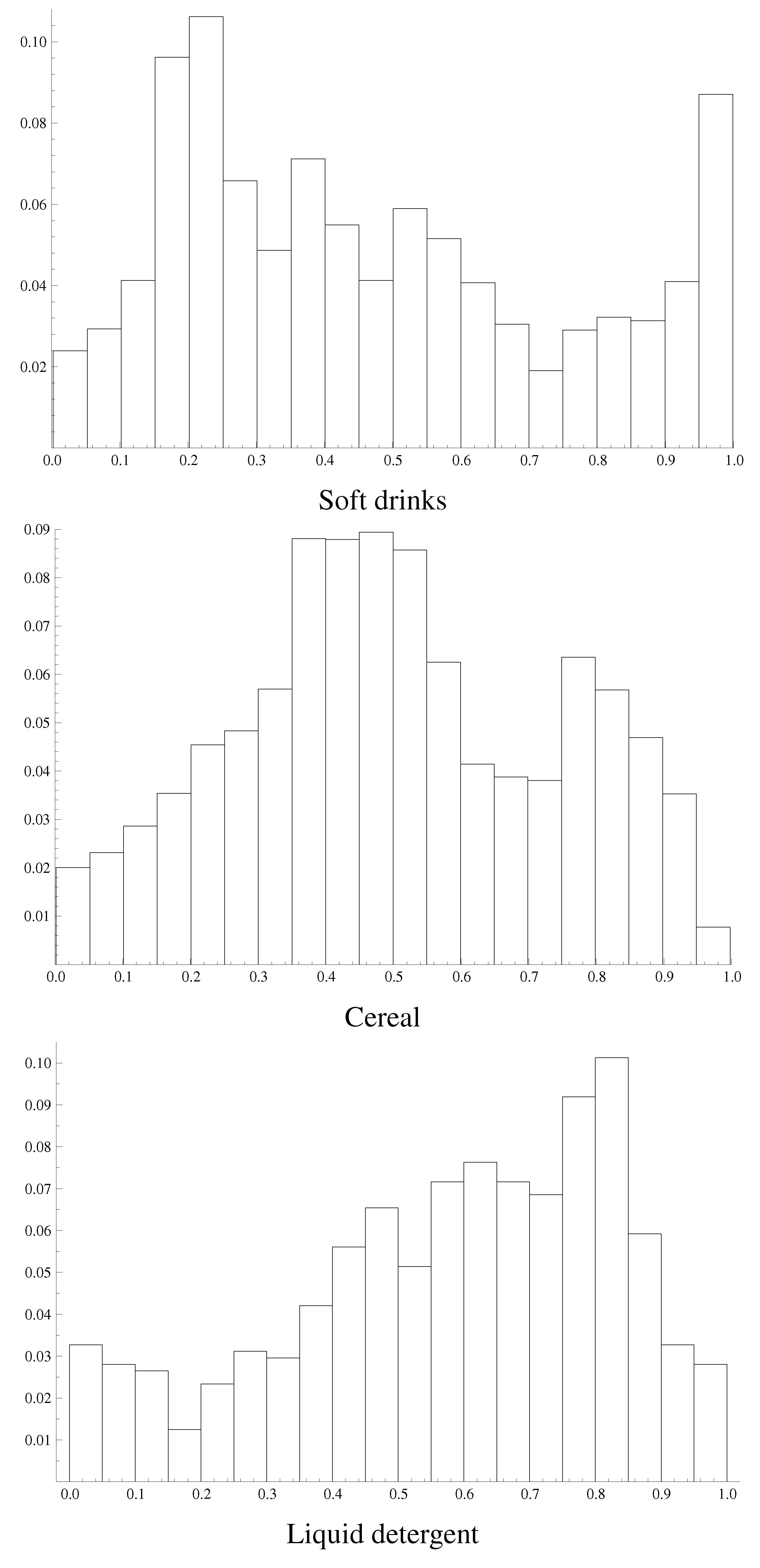
Figure 1 displays histograms of the posterior means of the responsiveness probabilities per purchase occasion (
11). Across the three categories, we see quite a bit of differences. For soft drinks, we find a relatively large proportion of purchase trips at which the household was responsive with a probability of almost one. We also find a cluster of observations with around a 0.2 probability of being responsive. For the cereal category, the probabilities are more centered around 0.5. For the liquid detergents, the distribution of the posterior probabilities is much more skewed to the right. Out of the three categories, the households act most responsive here.
Figure 1.
Histograms of the posterior means of the responsiveness probabilities.
Figure 1.
Histograms of the posterior means of the responsiveness probabilities.
The differences in these graphs may be explained from the characteristics of the shopping trips. The data show that the average inter-purchase times for liquid detergents are more than two times higher than for the other categories. A higher inter-purchase time may imply that households are relying less on routine to make the choice. Therefore, they may not be able to remember past prices and may be more actively involved with the purchase. As a result, households may be more likely to search for price information. The average inter-purchase time in the soft drinks categories is the smallest. Households are more likely to rely on memory, and they are less responsive. Additionally, we see that the average amount of dollars spent on the shopping trips involving soft drinks is smaller than for purchases in the other categories. This may imply that households have more time to compare prices when their shopping basket is smaller. The combination of both effects may explain the bimodality in the responsiveness distribution in the soft drinks category, as shown in the first panel of
Figure 1. The results for the cereal category are somewhere in between with respect to the average inter-purchase times and the average amount of dollars spent.
To see the difference in cross-sectional variation in responsiveness and temporal variation, we compute the ratio of the average of the variance of the responsiveness probabilities per household to the variance of the average responsiveness probability per household. This ratio is 0.34 for the soft drinks category. For the cereal and detergent category, the ratios equal 12.32 and 1.51, respectively. Hence, for the latter two categories, the within household spread in response probabilities is larger than the spread across households. The difference between the smallest and largest responsiveness probability per household shows that for 87% of the households, this difference is larger than 50%, indicating that there is within-household variation in the responsiveness state. For the soft drinks and liquid detergent category, these percentages are 60% and 40%, respectively.
The histograms in
Figure 1 do not provide direct information on which type of household is responsive at which type of shopping trip. Such information can, however, be obtained from the parameter estimates related to responsiveness Equation (
2).
Table 2 displays the posterior results for the complete responsiveness model. We carried out a limited model selection exercise to fine-tune the models. Based on overwhelming support of a Bayes factor, we have restricted the display variable to zero in the responsive choice part of the model for soft drinks and cereal.
The final line of
Table 2 again confirms that the average responsiveness probability is close to 50%. This again stresses the importance of the unresponsive segment, as in fact, about half of the purchases can be associated with this segment. Furthermore, it shows that for liquid detergents, the households tend to be most responsive.
The first panel of
Table 2 shows the parameters that influence the responsiveness state. The household size is positively related to the responsiveness to marketing efforts for soft drinks and liquid detergents. For cereals, this effect is also positive, but the effect is close to zero. For cereals, family income is a more important driver, where here, a higher family income implies less responsiveness. Note that the influence of lagged choice for cereal is small in the brand choice model for the unresponsive state. Hence, households with a higher income are more likely to go for their favorite brand without considering price. For soft drinks, we find that a longer inter-purchase time leads to a higher responsiveness probability. A longer inter-purchase time implies a higher need to actively compare the brands, as the last purchase cannot be remembered easily. This contradicts the idea that frequent buyers do more price checking [
15]. Time since the last purchase is also positive for the cereal and liquid detergent category, but the posterior means are about the same as the posterior standard deviation. The average inter-purchase time in these categories is in general higher than for the soft drinks category, and a longer or shorter than average inter-purchase time possibly does not influence the probability of being responsive anymore.
Table 2.
Posterior results for the responsiveness model .
Table 2.
Posterior results for the responsiveness model .
| | Soft drinks | Cereal | Liquid detergent |
|---|
| Variable | mean | SD | mean | SD | mean | SD |
|---|
| Probit equation being responsive (3) |
| intercept | 0.069 | 0.063 | 0.019 | 0.021 | 0.247 | 0.220 |
| household size | 0.916 *** | 0.384 | 0.062 | 0.086 | 0.625 *** | 0.215 |
| family income | 0.115 | 0.206 | -0.140* | 0.076 | -0.061 | 0.221 |
| dollars spent | 0.131 | 0.131 | 0.058 | 0.052 | -0.310 * | 0.182 |
| weeks since last purchase | 0.229 ** | 0.110 | 0.048 | 0.042 | 0.153 | 0.157 |
| Utility equation being responsive (5) |
| brand 1 | -0.211 | 0.201 | 3.110 *** | 0.249 | 1.227 * | 0.622 |
| brand 2 | -0.205 | 0.233 | 2.759 *** | 0.271 | -0.353 | 0.758 |
| brand 3 | 0.258 | 0.217 | 2.117 *** | 0.262 | 0.804 | 0.560 |
| brand 4 | -0.562 ** | 0.288 | 1.832 *** | 0.314 | -0.540 | 0.748 |
| brand 5 | 0.134 | 0.172 | 0.217 | 0.367 | 1.255 ** | 0.579 |
| brand 6 | -1.327 *** | 0.513 | | | 0.113 | 0.771 |
| lagged choice | 0.089 * | 0.053 | 0.256 ** | 0.092 | 1.875 *** | 0.383 |
| price | -0.342 *** | 0.098 | -0.159 *** | 0.063 | -0.523 | 0.312 |
| feature | 0.126 ** | 0.057 | 0.165 *** | 0.043 | 0.565 ** | 0.223 |
| display b | | | | | 0.541 ** | 0.220 |
| Utility equation being unresponsive (7) |
| brand 1 | -0.037 | 0.336 | 0.961 *** | 0.341 | -0.369 | 0.618 |
| brand 2 | 0.552 * | 0.326 | 2.121 *** | 0.162 | 0.057 | 0.464 |
| brand 3 | 0.980 *** | 0.379 | 0.824 *** | 0.237 | -1.579 ** | 0.808 |
| brand 4 | 0.593 | 0.364 | 0.714 *** | 0.225 | -1.444 | 1.025 |
| brand 5 | 0.300 | 0.309 | 0.393 ** | 0.168 | -0.174 | 0.907 |
| brand 6 | 0.071 | 0.453 | | | 1.181 *** | 0.449 |
| lagged choice | 0.510 *** | 0.070 | 0.036 | 0.090 | 0.514 ** | 0.252 |
| average responsiveness | 0.475 | 0.507 | 0.582 |
| probability |
In [
35], the authors find that larger basket sizes tend to be purchased at everyday, low-price stores, implying that households do respond to price. In this paper, however, we consider the influence of basket size on price responsiveness given store choice, which may have the opposite effect, as a large shopping basket may mean that less time can be devoted to each particular category, which, in turn, makes the household less responsive. In fact, for liquid detergents, we find that a larger basket size leads to a smaller probability of being responsive. For the other two categories, we find the opposite results, but the posterior means are about the same as the posterior standard deviation. In general, the amount of dollars spent on shopping trips containing cereal and soft drinks turn out to be smaller than for shopping trips containing purchases of liquid detergents, which may explain the difference.
The second and third panel of
Table 2 present the parameter estimates for the brand utilities. The results indicate that there can be substantial differences in the baseline preferences across the responsive and the unresponsive segment. For example, for soft drinks, brand 3 has an average baseline preference within the responsiveness segment, but a relatively large baseline preference within the unresponsive segment.
The influence of lagged choice also differs substantially across the two segments. For cereal and detergents, we find that lagged choice is not important for unresponsive households; for soft drinks, we however find the opposite. If we consider the posterior means of the brand intercepts, we see that the differences in values across the brands is large for the cereal and liquid detergents category. Households seem to have a more distinct preference for a brand in these two categories. On unresponsive purchase occasions, they are more likely to choose their favorite brand, and lagged choice plays a less important role. For the soft drinks category, the differences in posterior means in the brand intercepts is much smaller, and lagged choice seems to be more important if the actual price does not matter.
Finally, the posterior means of the marketing-mix variables have the expected sign for all three product categories. The effect of price is negative, and for feature and display, we find a positive effect.
Unreported estimates of the variance of the brand intercepts (
) and the variance of the marketing-mix variables (
) show that there is substantial variation in base preferences and marketing-mix parameters. Overall, the variation in the base preferences is largest. Comparing the different categories, we find that the heterogeneity is largest for detergents and that the degree of heterogeneity is about equal for cereal and soft drinks
2.
4.2. Standard MNP Model
The results in
Table 2 already indicated that models for responsive and non-responsive households can differ, and the consequences of this finding are further articulated by the estimation results for the MNP model in
Table 3. Most noticeable are the differences in coefficients for price. While the posterior mean of the price parameter for the responsive households are
,
and
across the three categories, the MNP model for all households would yield an underestimation of the price effect as
,
and
, respectively, which, on average, implies an underestimation of around
. Note that in this MNP model, we also allow for heterogeneity across households. The responsiveness model clearly allows us to additionally separate the responsive from the unresponsive purchase occasions. Of course, when we do not make this split, the average price elasticity will be severely affected.
Table 3.
Posterior results for the multinomial probit (MNP) model (
20)
.
Table 3.
Posterior results for the multinomial probit (MNP) model (20) .
| | Soft drinks | Cereal | Liquid detergent |
|---|
| Variable | mean | SD | mean | SD | mean | SD |
|---|
| brand 1 | -0.100 | 0.177 | 1.920 *** | 0.168 | 0.647 * | 0.389 |
| brand 2 | 0.068 | 0.189 | 2.211 *** | 0.169 | -0.116 | 0.493 |
| brand 3 | 0.470 *** | 0.162 | 1.249 *** | 0.171 | -0.270 | 0.462 |
| brand 4 | -0.078 | 0.181 | 0.996 *** | 0.173 | -0.750 | 0.496 |
| brand 5 | 0.151 | 0.148 | 0.403 ** | 0.190 | 1.067 ** | 0.449 |
| brand 6 | -0.463 | 0.307 | | | 1.065 *** | 0.413 |
| lagged choice | 0.298 *** | 0.028 | 0.109 *** | 0.019 | 0.615 *** | 0.127 |
| price | -0.140 ** | 0.068 | -0.072 ** | 0.037 | -0.306 * | 0.164 |
| feature | 0.077 | 0.047 | 0.045 * | 0.024 | 0.255 ** | 0.116 |
| display | | | | | 0.290 ** | 0.123 |
The parameter concerning lagged choice is also different across the models in
Table 2 and
Table 3. The parameter values in the MNP model are smaller than the values in the responsive part for the cereal and liquid detergent category and is larger for the soft drinks category.
4.3. MNP Model with Cross Effects
One of the main differences between our responsiveness model and the “standard MNP model with heterogeneity” is that household variables do not interact with the marketing instruments. Of course, one could extend the MNP model with these interaction effects.
Table 4 reports the posterior results for such an MNP model.
Clearly, the results indicate that only a very minor additional contribution can be observed from these cross effects, except for a weak effect of the weeks since last purchase and feature for liquid detergent. The fact that we allow for unobserved heterogeneity in the effects of the marketing-mix variables already seems to sufficiently describe the differences in response to marketing-mix variables.
Taking the outcomes in
Table 2,
Table 3 and
Table 4 together, we can conclude that the responsiveness model seems to add an important feature to the choice model. Ignoring this feature leads to substantively different results. For example, the MNP model with or without cross effects underestimates price effects relative to our model.
Next, we will focus on the fit of the different models to see whether the responsiveness model indeed fits the data better.
Table 4.
Posterior results for the MNP model with cross effects .
Table 4.
Posterior results for the MNP model with cross effects .
| | Soft drinks | Cereal | Liquid detergent |
|---|
| Variable | mean | SD | mean | SD | mean | SD |
|---|
| brand 1 | -0.072 | 0.178 | 1.848 *** | 0.145 | 0.806 | 0.460 |
| brand 2 | 0.106 | 0.181 | 2.130 *** | 0.145 | -0.252 | 0.544 |
| brand 3 | 0.493 *** | 0.158 | 1.203 *** | 0.144 | -0.178 | 0.562 |
| brand 4 | -0.084 | 0.187 | 0.962 *** | 0.149 | -0.655 | 0.535 |
| brand 5 | 0.183 | 0.146 | 0.357 ** | 0.156 | 1.004 ** | 0.501 |
| brand 6 | -0.553 * | 0.320 | | | 1.153 ** | 0.537 |
| lagged choice | 0.296 *** | 0.028 | 0.114 *** | 0.019 | 0.606 *** | 0.134 |
| price | -0.133 ** | 0.064 | -0.063 * | 0.037 | -0.278 | 0.184 |
| feature | 0.081 * | 0.046 | 0.063 ** | 0.025 | 0.272 ** | 0.133 |
| display | | | | | 0.320 ** | 0.135 |
| Cross effect with household size |
| price | 0.012 | 0.066 | -0.023 | 0.041 | 0.078 | 0.215 |
| feature | -0.018 | 0.043 | -0.026 | 0.026 | 0.101 | 0.159 |
| display | | | | | 0.048 | 0.141 |
| Cross effect with family income |
| price | 0.008 | 0.066 | 0.054 | 0.038 | 0.200 | 0.196 |
| feature | -0.008 | 0.047 | 0.039 | 0.026 | -0.094 | 0.126 |
| display | | | | | -0.072 | 0.128 |
| Cross effect with dollars spent |
| price | -0.053 | 0.037 | 0.018 | 0.026 | 0.178 | 0.145 |
| feature | -0.014 | 0.020 | -0.024 | 0.017 | 0.110 | 0.103 |
| display | | | | | 0.016 | 0.107 |
| Cross effect with weeks since last purchase |
| price | -0.017 | 0.027 | 0.009 | 0.016 | 0.029 | 0.143 |
| feature | 0.000 | 0.016 | 0.006 | 0.012 | 0.134 * | 0.080 |
| display | | | | | -0.036 | 0.092 |
4.4. Model Comparison
In
Table 5, we present three fit measures for our three models, that is, the log predictive likelihood (
22), the hit rate and the mean squared prediction error (MSPE). The predictive likelihood functions of the responsiveness model are clearly larger than for the MNP model and the MNP model with cross effects for all product categories. Predictive odds ratios are clearly larger than 50 in favor of the responsiveness model, except for the cereal category, where we find an odds ratio of about three in favor of the responsiveness model compared to the MNP specification. Note that because this comparison is based on observations not used during estimation, we do not need to penalize for the number of parameters. Recall that we take the final purchase occasion for each household to form the test sample. Furthermore, note that the “standard MNP model” outperforms the MNP model with cross effects. Based on the results in
Table 4, this was to be expected, as hardly any cross effects turned out to be relevant.
Table 5.
Model comparison.
Table 5.
Model comparison.
| Model | Soft drinks | Cereal | Liquid detergent |
|---|
| Log predictive likelihood (22) |
| responsiveness | | | |
| MNP (20) | | | |
| MNP + cross (21) | | | |
| Hit rate |
| responsiveness | | | |
| MNP (20) | | | |
| MNP + cross (21) | | | |
| Mean squared prediction error a |
| responsiveness | | | |
| MNP (20) | | | |
| MNP + cross (21) | | | |
Looking at the (out-of-sample) hit rate, we find that, except for the cereal category, the responsiveness model also gives the highest hit rate. A closer look at the higher hit rate of the MNP model with cross effects for the cereal category shows that the higher hit rate is accompanied by higher prediction probabilities in the case that the model produces a mishit. This explains why the log predictive likelihood of the responsiveness model of cereal is higher. However, the differences in the hit rate across all models are negligible.
As a final performance measure, we consider the MSPE. In general, the MSPE of the responsiveness model is smallest. Note that the MSPE also indicates that the MNP model with cross effects performs worst.
The illustrations in this section have indicated quite convincingly that allowing for a possibly large fraction of non-responsive households leads to a better fit and to a more appropriate interpretation of the effects of market efforts, like price.
5. Concluding Remarks
Households may not respond to marketing-mix instruments at each purchase occasion. To be able to respond to these efforts, one needs to invest time and effort in, for example, remembering price changes and reading newspapers and leaflets to notice advertisements. Households differ in the amount of effort they wish to invest in a particular purchase, and therefore, they will most likely also differ in their responsiveness to marketing efforts.
The choice model we developed in this paper incorporates the responsiveness of a household at a specific purchase occasion as a form of unobserved heterogeneity. Households differ in their purchasing process. In essence, we assume there are two processes. Households either take marketing efforts into account, or they base their choice on base preferences and their past experiences. The specific decision process used can differ across households and across purchase occasions. To explain and forecast the decision process, used by a specific household at a specific purchase occasion, household characteristics can be used together with information on buying behavior. To take into account this form of heterogeneity, we extended a standard brand choice model. Basically, we introduced two segments of households, one segment is unresponsive to marketing efforts, whereas the other segment does respond to these efforts. The segment membership is separately modeled using a binary probit model. Household are allowed to switch over time between being responsive or not.
The illustration of our new model to three distinct categories shows that quite some different results can be obtained across our model and related MNP models. Some of the differences can be related to the circumstances and characteristics of the shopping trips in these product categories, such as inter-purchase times and the size of the shopping basket. Even though there were only three cases, we can draw a generalizing conclusion, and that is that the effects of market efforts will be underestimated in MNP models, as in these models, both responsive and non-responsive households are jointly treated as a single sample. Allowing for this specific form of heterogeneity in our model thus leads to better insights into the effects of the marketing mix. One can also identify the characteristics that result in higher probabilities of being responsive for households, and this has immediate managerial consequences. One key result of our model is that it leads to better targeting of marketing instruments, which, at the same time, then also yield less irritation and waste. Further research should examine if the responsiveness fraction of around 0.5 in the three studied categories is a fraction that could commonly be found for fast-moving consumer goods or whether such a fraction could differ across different types of products.

