Bias-Correction in Vector Autoregressive Models: A Simulation Study

Abstract

We analyze the properties of various methods for bias-correcting parameter estimates in both stationary and non-stationary vector autoregressive models. First, we show that two analytical bias formulas from the existing literature are in fact identical. Next, based on a detailed simulation study, we show that when the model is stationary this simple bias formula compares very favorably to bootstrap bias-correction, both in terms of bias and mean squared error. In non-stationary models, the analytical bias formula performs noticeably worse than bootstrapping. Both methods yield a notable improvement over ordinary least squares. We pay special attention to the risk of pushing an otherwise stationary model into the non-stationary region of the parameter space when correcting for bias. Finally, we consider a recently proposed reduced-bias weighted least squares estimator, and we find that it compares very favorably in non-stationary models.

1. Introduction

It is well-known that standard ordinary least squares (OLS) estimates of autoregressive parameters are biased in finite samples. Such biases may have important implications for models in which estimated autoregressive parameters serve as input. For example, small sample bias may severely distort statistical inference (Mark [1], Bekaert et al. [2], Kilian [3], Stambaugh [4], Lewellen [5], Amihud and Hurvich [6]), forecasting accuracy (Kim [7,8,9]), estimation of impulse response functions (Kilian [10,11], Patterson [12]), estimation of optimal portfolio choices in dynamic asset allocation models (Engsted and Pedersen [13]), and estimation of dynamic term structure models (Bauer et al. [14]).

Simple analytical formulas for bias-correction in univariate autoregressive models are given in Marriott and Pope [15], Kendall [16], White [17], and Shaman and Stine [18]. In particular, the bias in the simple univariate AR(1) model has been analyzed in many papers over the years using both analytical expressions, numerical computations, and simulations, e.g., Orcutt and Winokur [19], Sawa [20], MacKinnon and Smith [21], Patterson [22], and Bao and Ullah [23]. In a multivariate context analytical expressions for the finite-sample bias in estimated vector autoregressive (VAR) models have been developed by Tjøstheim and Paulsen [26], Yamamoto and Kunitomo [27], Nicholls and Pope [28], Pope [29], and Bao and Ullah [23]. However, there are no detailed analyses of the properties of these multivariate analytical bias formulas. If bias-adjustment using the analytical formulas has better or equally good properties compared to more computer intensive bootstrap bias-adjustment methods, this gives a strong rationale for using the analytical formulas rather than bootstrapping.

This paper investigates the properties of various bias-adjustment methods for VAR models.1 First, we show that the analytical bias expressions developed (apparently independently) by Yamamoto and Kunitomo [27] one the one hand and Nicholls and Pope [28] and Pope [29] on the other hand, are identical. To our knowledge this equivalence has not been noticed in the existing literature.2

Second, through a simulation experiment we investigate the properties of the analytical bias formula and we compare these properties with the properties of both standard OLS, Monte Carlo/bootstrap generated bias-adjusted estimates, and the weighted least squares approximate restricted likelihood (WLS) estimator recently developed by Chen and Deo [30], which should have reduced bias compared to standard least squares. We investigate both bias and mean squared error of these estimators. Since in general the bias depends on the true unknown parameter values, correcting for bias is not necessarily desirable because it may increase the variance, thus leading to higher mean squared errors compared to uncorrected estimates, cf., e.g., MacKinnon and Smith [21]. We investigate both a simple one-step ‘plug-in’ approach where the initial least squares estimates are used in place of the true unknown values to obtain the bias-adjusted estimates, and a more elaborate multi-step iterative scheme where we repeatedly substitute bias-adjusted estimates into the bias formulas until convergence. We also consider inverting the analytical bias formula, i.e., conditional on the least squares estimates we solve for the true parameter values using the bias formula and subsequently use these ‘true’ parameters to estimate thebias.

In many empirical applications the variables involved are highly persistent which may lead to both the least squares and the bias-adjusted VAR parameter matrix containing unit or explosive roots. Kilian [10] proposes a very simple method for eliminating non-stationary roots when bias-adjusting VAR parameter estimates. We investigate how the use of Kilian’s approach affects the finite-sample properties of the bias-correction methods. To secure stationary roots in the first step an often used alternative to OLS is the Yule-Walker estimator, which is guaranteed to deliver stationary roots. We investigate the finite-sample properties of this estimator and we compare it to OLS both with and without bias correction. We also consider non-stationary systems. The analytical bias formula is derived under the assumption of stationarity, while WLS allows for unit roots, which suggests that WLS should be the preferred choice of estimator in this scenario.

Finally, we analyze the finite-sample properties of bias-correction methods (both bootstrap and analytical methods) in the presence of skewed and fat-tailed data, and we compare a parametric bootstrap procedure, based on a normal distribution, with a residual-based bootstrap procedure when in fact data are non-normal. Among other things, this analysis will shed light on the often used practice in empirical studies of imposing a normal distribution when generating bootstrap samples from parameter values estimated on non-normal data samples. Furthermore, in contrast to the analytical bias formula WLS is derived using a normality assumption. We include WLS in the comparison based on non-normal data to evaluate if violation of the normality assumption distorts the finite-sample properties of the estimator.3

The rest of the paper is organized as follows. In the next section we present the various bias-correction methods, based on either a bootstrap procedure or analytical bias formulas, and the reduced-bias WLS estimator. Section 3 reports the results of the simulation study where we analyze and compare the properties of the different bias-correction methods. Section 4 contains a summary of the results.

2. Bias-Correction in a VAR model

In this section we discuss ways to correct for the bias of least squares estimates of VAR parameters. For simplicity, we here only consider the VAR(1) model

$$Y_t=\theta +\mathrm{\Phi }{Y}_{t-1}+u_t,t=1,...,T$$

(1)

where $Y_t$ and $u_t$ are $k\times 1$ vectors consisting of the dependent variable and the innovations, respectively. θ is a $k\times 1$ vector of intercepts and Φ is a $k\times k$ matrix of slope coefficients. The covariance matrix of the innovations, which are independent and identically distributed, is given by the $k\times k$ matrix ${\mathrm{\Omega }}_u$. Alternatively, if the intercept is of no special interest the VAR(1) model can be formulated in a mean-corrected version as

$$X_t=\mathrm{\Phi }{X}_{t-1}+u_t,t=1,...,T$$

(2)

where $X_t=Y_t-\mu$ with $\mu ={\left(I_k-\mathrm{\Phi }\right)}^{-1}\theta$. Higher-order VAR models can be stated in first-order form by using the companion form, so the focus on VAR(1) models is without loss of generality. We consider both stationary VAR models and models with unit roots.

2.1. Bootstrap Bias-Correction

Usually, in applied econometrics bias-adjustment is done using Monte Carlo or bootstrap procedures. The general procedure in bias-adjusting the OLS estimate of Φ can be summarized as follows for the VAR(1) model in (2):4

• Estimate the VAR model (2) using OLS. Denote this estimate $\widehat{\mathrm{\Phi }}$.
• Conditional on $\widehat{\mathrm{\Phi }}$ simulate M bootstrap samples (each of size T). This step requires simulation of the innovations $u_t$, which can be done either by repeated sampling with replacement from the residuals from step 1 or by sampling from an assumed parametric distribution.
• For each bootstrap sample estimate (2) using OLS. Denote this estimate ${\widehat{\mathrm{\Phi }}}^{*}$. Calculate the average of ${\widehat{\mathrm{\Phi }}}^{*}$ across the M bootstrap samples. Denote the average by $\overline{\mathrm{\Phi }}$.
• Calculate the estimate of the bias as $B_T^B=\overline{\mathrm{\Phi }}-\widehat{\mathrm{\Phi }}$, or accordingly the bias-adjusted estimate of Φ as $2\widehat{\mathrm{\Phi }}-\overline{\mathrm{\Phi }}$.

2.2. Analytical Bias Formulas

As an alternative to bootstrapping there also exist analytical bias formulas, which provide an easy and simple approach to bias-adjustment in VAR models. Yamamoto and Kunitomo [27] derive analytical expressions for the bias of the least squares estimator in VAR models. Based on model (1), Yamamoto and Kunitomo derive the following expression for the asymptotic bias of the OLS estimator of the slope coefficient matrix Φ

$$B_T^{YK}=-\frac{b^{YK}}{T}+O\left(T^{-3/2}\right),$$

(3)

where

$$b^{YK}={\mathrm{\Omega }}_u\sum _{i=0}^{\infty }\left[{\left({\mathrm{\Phi }}^{\prime }\right)}^i+{\left({\mathrm{\Phi }}^{\prime }\right)}^{i}tr\left({\mathrm{\Phi }}^{i+1}\right)+{\left({\mathrm{\Phi }}^{\prime }\right)}^{2i+1}\right]{\left[\sum _{j=0}^{\infty }{\mathrm{\Phi }}^j{\mathrm{\Omega }}_u{\left({\mathrm{\Phi }}^{\prime }\right)}^j\right]}^{-1}.$$

(4)

Yamamoto and Kunitomo also show that the asymptotic bias of the OLS estimator of the intercept θ follows by post-multiplying $b^{YK}$ by $-{\left(I_k-\mathrm{\Phi }\right)}^{-1}\theta$.

The bias expression is derived under the assumption that the innovations are independent and identically distributed with covariance matrix ${\mathrm{\Omega }}_u$, and that the VAR system is stationary such that Φ does not contain unit or explosive roots. A few additional assumptions are required (see Yamamoto and Kunitomo [27] for details), and it can be noted that a sufficient but not necessary condition for these assumptions to be satisfied is Gaussian innovations. The finite-sample error in the bias formula vanishes at the rate $T^{-3/2},$ which is at least as fast as in standard Monte Carlo or bootstrap bias-adjustment.

Yamamoto and Kunitomo also derive the asymptotic bias of the slope coefficient matrix in the special case where $\theta =0$:

$$b_{\theta =0}^{YK}={\mathrm{\Omega }}_u\sum _{i=0}^{\infty }\left[{\left({\mathrm{\Phi }}^{\prime }\right)}^{i}tr\left({\mathrm{\Phi }}^{i+1}\right)+{\left({\mathrm{\Phi }}^{\prime }\right)}^{2i+1}\right]{\left[\sum _{j=0}^{\infty }{\mathrm{\Phi }}^j{\mathrm{\Omega }}_u{\left({\mathrm{\Phi }}^{\prime }\right)}^j\right]}^{-1}.$$

(5)

Compared to the case with intercept, the term ${\left({\mathrm{\Phi }}^{\prime }\right)}^i$ is no longer included in the first summation. This illustrates the general point that the bias of slope coefficients in autoregressive models is smaller in models without intercept than in models with intercept, see e.g. Shaman and Stine [18] for the univariate case. In a univariate autoregressive model the above bias expressions can by simplified. For example, in an AR(1) model, $y_t=\alpha +\rho y_{t-1}+{\epsilon }_t$, the bias of the OLS estimator of ρ is given by $-\left(1+3\rho \right)/T,$ which is consistent with the well-known expression by Kendall [16]. If $\alpha =0$ the bias of the OLS estimator of ρ is given by $-2\rho /T,$ which is consistent with the work by White [17].

Based on the VAR model (2) Pope [29] derives the following analytical bias formula for the OLS estimator of the slope coefficient matrix Φ

$$B_T^P=-\frac{b^P}{T}+O\left(T^{-3/2}\right),$$

(6)

where

$$b^P={\mathrm{\Omega }}_u\left[{\left(I_k-{\mathrm{\Phi }}^{\prime }\right)}^{-1}+{\mathrm{\Phi }}^{\prime }{\left(I_k-{\left({\mathrm{\Phi }}^{\prime }\right)}^2\right)}^{-1}+\sum _{i=1}^k{\lambda }_i{\left(I_k-{\lambda }_i{\mathrm{\Phi }}^{\prime }\right)}^{-1}\right]{\mathrm{\Omega }}_x^{-1}.$$

(7)

${\lambda }_i$ denotes the i’th eigenvalue of Φ and ${\mathrm{\Omega }}_x$ is the covariance matrix of $X_t$. Pope obtains this expression by using a higher-order Taylor expansion and, as seen, the approximation error in the bias formula vanishes at the rate $T^{-3/2}$, which is of the same magnitude as the finite-sample error in Yamamoto and Kunitomo’s asymptotic bias formula. The underlying assumptions are quite mild (see Pope [29] for details). Among the assumptions are that the VAR system is stationary, and that the VAR innovations $u_t$ constitute a martingale difference sequence with constant covariance matrix ${\mathrm{\Omega }}_u$. The expression does not, however, require Gaussian innovations.5

By comparing the two expressions (4) and (7) we see that they appear very similar and, in fact, they turn out to be identical as stated in Theorem 1:

Theorem. The analytical bias formulas by Yamamoto and Kunitomo [27] and Pope [29] are identical since $b^P=b^{YK}.$

Proof. We can rewrite the infinite sums in $b^{YK}$ as follows

$$\begin{array}{cc}\hfill \sum _{i=0}^{\infty }{\left({\mathrm{\Phi }}^{\prime }\right)}^i& ={\left(I_k-{\mathrm{\Phi }}^{\prime }\right)}^{-1}\hfill \\ \hfill \sum _{i=0}^{\infty }{\left({\mathrm{\Phi }}^{\prime }\right)}^{2i+1}& ={\mathrm{\Phi }}^{\prime }\sum _{i=0}^{\infty }{\left({\mathrm{\Phi }}^{\prime }\right)}^{2i}={\mathrm{\Phi }}^{\prime }{\left(I_k-{\left({\mathrm{\Phi }}^{\prime }\right)}^2\right)}^{-1}\hfill \\ \hfill \sum _{i=0}^{\infty }{\mathrm{\Phi }}^i{\mathrm{\Omega }}_u{\left({\mathrm{\Phi }}^{\prime }\right)}^i& =E\left[\left(Y_t-\mu \right){\left(Y_t-\mu \right)}^{\prime }\right]=E\left[X_t{X}_t{}^{\prime }\right]={\mathrm{\Omega }}_x\hfill \\ \hfill \sum _{i=0}^{\infty }{\left({\mathrm{\Phi }}^{\prime }\right)}^{i}tr\left({\mathrm{\Phi }}^{i+1}\right)& =\sum _{i=0}^{\infty }{\left({\mathrm{\Phi }}^{\prime }\right)}^i\left({\lambda }_1^{i+1}+...+{\lambda }_k^{i+1}\right)\hfill \\ & ={\lambda }_1\sum _{i=0}^{\infty }{\left({\mathrm{\Phi }}^{\prime }\right)}^i{\lambda }_1^i+...+{\lambda }_k\sum _{i=0}^{\infty }{\left({\mathrm{\Phi }}^{\prime }\right)}^i{\lambda }_k^i\hfill \\ & ={\lambda }_1{\left(I_k-{\lambda }_1{\mathrm{\Phi }}^{\prime }\right)}^{-1}+...+{\lambda }_k{\left(I_k-{\lambda }_k{\mathrm{\Phi }}^{\prime }\right)}^{-1}\hfill \\ & =\sum _{j=1}^k{\lambda }_j{\left(I_k-{\lambda }_j{\mathrm{\Phi }}^{\prime }\right)}^{-1},\hfill \end{array}$$

where $X_t=Y_t-\mu$ with $\mu ={\left(I_k-\mathrm{\Phi }\right)}^{-1}\theta$ and ${\lambda }_i$ denotes the i’th eigenvalue of Φ.    ☐

In applying (4), Yamamoto and Kunitomo [27] suggest to truncate the infinite sums by taking the summation from 0 to T, based on the argument that the remaining terms are of the order $o\left(T^{-1}\right)$. However, due to the equivalence of (4) and (7) there is no need to apply (4) with such a truncation. In practice the formula in (7) should be used.

In contrast to Yamamoto and Kunitomo [27], Pope [29] does not consider the bias in the estimated intercepts $\widehat{\theta }$ or in the special case where $\theta =0$ but from Theorem 1 we obtain the following results:

Corollary. The bias in the OLS estimate of θ is given by (6) with

$$b^P=-{\mathrm{\Omega }}_u\left[{\left(I_k-{\mathrm{\Phi }}^{\prime }\right)}^{-1}+{\mathrm{\Phi }}^{\prime }{\left(I_k-{\left({\mathrm{\Phi }}^{\prime }\right)}^2\right)}^{-1}+\sum _{i=1}^k{\lambda }_i{\left(I_k-{\lambda }_i{\mathrm{\Phi }}^{\prime }\right)}^{-1}\right]{\mathrm{\Omega }}_x^{-1}{\left(I_k-\mathrm{\Phi }\right)}^{-1}\theta ,$$

and the bias in the OLS estimate of Φ with $\theta =0$ is given by (6) with

$$b_{\theta =0}^P={\mathrm{\Omega }}_u\left[{\mathrm{\Phi }}^{\prime }{\left(I_k-{\left({\mathrm{\Phi }}^{\prime }\right)}^2\right)}^{-1}+\sum _{i=1}^k{\lambda }_i{\left(I_k-{\lambda }_i{\mathrm{\Phi }}^{\prime }\right)}^{-1}\right]{\mathrm{\Omega }}_x^{-1}.$$

2.3. Ensuring Stationarity

An important problem in adjusting for bias using bootstrap and the analytical bias formula is that the bias-adjusted estimate of Φ may fall into the non-stationary region of the parameter space. The analytical bias formula is derived under the assumption of stationarity and, hence, the presence of unit or explosive roots will be inconsistent with the underlying premise for the VAR system we are analyzing. Kilian [10] suggests an approach to ensure that we always get a bias-adjusted estimate that does not contain unit or explosive roots. This approach is used by, e.g., Engsted and Tanggaard [31] and Engsted and Pedersen [13] and is as follows: First, estimate the bias and obtain a bias-adjusted estimate of Φ by subtracting the bias from the OLS estimate. Second, check if the bias-adjusted estimate falls within the stationary region of the parameter space. If this is the case, use this bias-adjusted estimate. Third, if this is not the case correct the bias-adjusted estimate by multiplying the bias with a parameter $\kappa \in \left[0,0.01,0.02,...,0.99\right]$ before subtracting it from the OLS estimate. This will ensure that the bias-adjusted estimate is within the stationary region of the parameter space.

Related to the issue of ensuring stationarity, how should we tackle bias-correction if the use of OLS leads to a non-stationary system when we know or suspect (perhaps based on economic theory) that the true VAR system is stationary? A potential solution is to use the Yule-Walker (YW) estimator, which is guaranteed to ensure a stationary system. However, YW has a larger bias than OLS and, hence, the finite-sample properties might be considerably worse. Pope [29] derives the bias of the YW estimator of the slope coefficient matrix Φ in (2) as

$$B_T^{YW}=-\frac{b^{YW}}{T}+O\left(T^{-3/2}\right),$$

(8)

where

$$b^{YW}=\mathrm{\Phi }+{\mathrm{\Omega }}_u\left[{\left(I_k-{\mathrm{\Phi }}^{\prime }\right)}^{-1}+{\mathrm{\Phi }}^{\prime }{\left(I_k-{\left({\mathrm{\Phi }}^{\prime }\right)}^2\right)}^{-1}+\sum _{i=1}^k{\lambda }_i{\left(I_k-{\lambda }_i{\mathrm{\Phi }}^{\prime }\right)}^{-1}\right]{\mathrm{\Omega }}_x^{-1}.$$

(9)

The approach and assumptions are identical to those used by Pope to derive the bias of the OLS estimator.6 Comparing this result to (7) we see that $b^{YW}=\mathrm{\Phi }+b^P$. In an AR(1) model, $y_t=\alpha +\rho y_{t-1}+{\epsilon }_t$, the bias of the YW estimator of ρ can be simplified to $-\left(1+4\rho \right)/T$. Hence, applying YW instead of OLS ensures stationarity but increases the bias. However, since we have an analytical bias formula for the YW estimator we can correct for bias in the same way as we would do for OLS.

2.4. Reduced-Bias Estimators

As an alternative to estimating the VAR model using OLS and subsequently correct for bias using the procedures outlined above, it is also possible to use a different estimation method that has better bias properties than OLS. In recent work, Chen and Deo [30] propose a weighted least squares approximate restricted likelihood (WLS) estimator of the slope coefficient matrix in a VAR(p) model with intercept, which has a smaller bias than OLS. In fact, they show that this estimator has bias properties similar to that of the OLS estimator without intercept. The estimator for a VAR(1) model is given as

$$\begin{array}{cc}\hfill vec\left({\mathrm{\Phi }}_{WLS}\right)& ={\left[\sum _{t=2}^T{L}_t{L}_t^{\prime }\otimes {\mathrm{\Omega }}_u^{-1}+U{U}^{\prime }\otimes {\mathrm{\Omega }}_u^{-1/2}{\left(I_k+D^{\prime }{\mathrm{\Omega }}_{u}D\right)}^{-1}{\mathrm{\Omega }}_u^{-1/2}\right]}^{-1}\hfill \\ & \times vec\left[{\mathrm{\Omega }}_u^{-1}\sum _{t=2}^T\left(Y_t-{\overline{Y}}_{\left(1\right)}\right)L_t^{\prime }+{\mathrm{\Omega }}_u^{-1/2}{\left(I_k+D^{\prime }{\mathrm{\Omega }}_{u}D\right)}^{-1}{\mathrm{\Omega }}_u^{-1/2}R{U}^{\prime }\right],\hfill \end{array}$$

(10)

where $L_t^{\prime }={\left(Y_{t-1}-{\overline{Y}}_{\left(0\right)}\right)}^{\prime },$ $U^{\prime }={\left(T-1\right)}^{-1/2}{\sum }_{t=2}^T{\left(Y_{t-1}-Y_1\right)}^{\prime },$ $R={\left(T-1\right)}^{-1/2}{\sum }_{t=2}^T\left(Y_t-Y_1\right),$ $D^{\prime }={\left(T-1\right)}^{1/2}{\left(I_k-\mathrm{\Phi }\right)}^{\prime }{\mathrm{\Omega }}_u^{-1/2},$ ${\overline{Y}}_{\left(0\right)}={\left(T-1\right)}^{-1}{\sum }_{t=2}^T{Y}_{t-1},$ and ${\overline{Y}}_{\left(1\right)}={\left(T-1\right)}^{-1}{\sum }_{t=2}^T{Y}_t$.

The weighted least squares estimator is derived under the assumption that the innovations are independent and normally distributed with constant covariance matrix ${\mathrm{\Omega }}_u$. The estimator is based on the restricted likelihood, which is derived under the assumption that the initial value is fixed, which in turn implies that the estimator allows for unit roots.

2.5. Unknown Parameter Values

Both the analytical bias formulas and the WLS estimator require knowledge of ${\mathrm{\Omega }}_u$ and $\mathrm{\Phi },$ which are unknown. Chen and Deo [30] suggest to estimate these using any consistent estimator such as OLS, and then use these consistent estimates instead. The same approach is typically used when applying the analytical bias formulas, see, e.g., Engsted and Pedersen [13]. We will denote this approach the ‘plug-in’ approach. Alternatively, we can apply a more elaborate iterative scheme in which bias-adjusted estimates of Φ are recursively inserted in (7) or (10), see, e.g., Amihud and Hurvich [6] and Amihud et al. [32]. An iterative scheme is basically just an extension of the ‘plug-in’ approach and could for the analytical bias formulas go as follows. First, reestimate the covariance matrix of the innovations, ${\mathrm{\Omega }}_u$, after adjusting for bias using the ‘plug-in’ approach and then substitute this covariance matrix into the formulas together with the bias-adjusted slope coefficients obtained from the ‘plug-in’ approach. This yields another set of bias-adjusted estimates, which we can then use to reestimate the covariance matrix and the bias. We can continue this procedure until the slope coefficient estimates converge. A similar approach can be used for the WLS estimator.

Alternatively, conditional on the OLS estimates we can solve for Φ (and thereby also ${\mathrm{\Omega }}_u$) in the analytical bias formulas. In the simple AR(1) model, $y_t=\alpha +\rho y_{t-1}+{\epsilon }_t$, where the bias of the OLS estimator, $\widehat{\rho },$ of ρ is given by $\widehat{\rho }-\rho =-\left(1+3\rho \right)/T$ it is easy to see that $\rho =\left(T\widehat{\rho }+1\right)/\left(T-3\right)$, which we can then insert back into the bias formula to obtain an estimate of the bias in $\widehat{\rho }$. This approach is related to the median-unbiased estimator by Andrews [33], which entails inverting the bias function.7 In the VAR(1) model this approach entails solving k highly nonlinear equations for k unknown parameters, which can be done relatively easy using numerical optimization routines.

3. Simulation Study

The general simulation scheme goes as follows. We perform 10,000 simulations for a number of different stationary VAR(1) models and for a number of different sample sizes. In each simulation we draw the inital values of the series from a multivariate normal distribution with mean ${\left(I_k-\mathrm{\Phi }\right)}^{-1}\theta$ and covariance matrix $vec\left({\mathrm{\Omega }}_x\right)={(I_{k\times k}-\mathrm{\Phi }\otimes \mathrm{\Phi })}^{-1}vec\left({\mathrm{\Omega }}_u\right)$. Likewise, the innovations are drawn randomly from a multivariate normal distribution with mean 0 and covariance matrix ${\mathrm{\Omega }}_u$. Based on the initial values and innovations we simulate the series forward in time until we have a sample of size T. For each simulation we estimate a VAR(1) model using OLS and WLS. Furthermore, we correct the OLS estimate for bias using the analytical bias formula (6) (denoted ABF) and using a bootstrap procedure (denoted BOOT). Based on the 10,000 simulations we calculate the mean slope coefficients, bias, variance, and root mean squared error (RMSE) for each approach. The bootstrap procedure follows the outline presented in Section 2.1. The innovations are drawn randomly with replacement from the residuals, and we also randomly draw initial values from the simulated data. This procedure is repeated 1,000 times for each simulation.8 Regarding the analytical bias formula and WLS, we use the ‘plug-in’ approach, cf. Section 2.5. In the analytical bias formula we calculate the covariance matrix of $X_t$ as $vec({\widehat{\mathrm{\Omega }}}_x)={(I_{k\times k}-\widehat{\mathrm{\Phi }}\otimes \widehat{\mathrm{\Phi }})}^{-1}vec({\widehat{\mathrm{\Omega }}}_u)$. In both the analytical bias formula and bootstrapping we ensure stationarity by applying the approach by Kilian [10], cf. Section 2.3. In using this approach we choose the largest value of κ that ensures that the bias-adjusted estimate no longer contains unit or explosive roots.

We deviate from this general scheme in a number of different ways, all of which will be clearly stated in the text. In Section 3.1 we also allow for a fixed initial value, since the WLS estimator is based on the restricted likelihood, which is derived under the assumption that the initial value is fixed. In Section 3.2 we investigate the effect of iterating on WLS and ABF and inverting ABF. In Section 3.3 we analyze the consequences of not using Kilian’s [10] approach to ensure stationarity and the properties of the YW estimator. In Section 3.4 we allow for VAR(1) models with unit roots. In Section 3.5 we investigate the finite-sample properties when data are skewed and fat-tailed instead of normally distributed, and we analyze the consequences of using a parametric bootstrap approach to adjust for bias using a wrong distributional assumption.

3.1. Bias-Correction in Stationary Models

Table 1 reports the simulation results for the following VAR(1) model

$$\theta =\left[\begin{array}{c}0\\ 0\end{array}\right],\mathrm{ }\mathrm{\Phi }=\left[\begin{array}{cc}0.80& 0.10\\ 0.10& 0.85\end{array}\right],\mathrm{ }{\mathrm{\Omega }}_u=\left[\begin{array}{cc}2& 1\\ 1& 2\end{array}\right],\mathrm{ }$$

(11)

where the eigenvalues of Φ are 0.722 and 0.928. This VAR model is also used in simulation studies by Amihud and Hurvich [6] and Amihud et al. [32] in analyzing return predictability by persistent state variables. The table shows the mean slope coefficients and the average squared bias, variance, and RMSE $=\sqrt{{\text{bias}}^2\text{+variance}}$ across the four slope coefficients for $T=\left\{50,100,200,500\right\}$. For expositional purposes bias${}^2$ and variance are multiplied by 100. The final column shows the number of simulations in which the approach results in an estimate of Φ in the non-stationary region of the parameter space. For example, for $T=50$ using OLS to estimate the VAR(1) model implies that 25 out of 10,000 simulations result in a non-stationary model. The estimates from these 25 simulations are included in the reported numbers. When the OLS estimate is in the non-stationary region of the parameter space, we do not perform any bias-adjustment and set the bias-adjusted estimate equal to the (non-stationary) OLS estimate. This implies that in 25 simulations the (non-stationary) OLS estimate is included in the numbers for ABF and BOOT. For these bias-adjustment procedures the number in the final column shows the number of simulations where OLS yields a stationary model, but where the bias-adjustment procedure pushes the model into the non-stationary region of the parameter space, and we use the approach by Kilian [10] to ensure a stationary model.

Table 1. Bias-correction in a stationary but persistent VAR(1) model. The results in this table are based on 10,000 simulations from the VAR(1) model given in (11). Bias${}^2$, variance, and RMSE are reported as the average across the four slope coefficients. Average bias${}^2$ and variance are multiplied by 100. The final column (#NS) gives the number of simulations that result in a VAR(1) system in the non-stationary region. OLS are ordinary least squares estimates; WLS are estimates based on equation (8); ABF are bias-adjusted estimates based on the analytical bias formula, equation (7); BOOT are bias-adjusted estimates based on the bootstrap.

		Mean Slope Coefficients
		${\mathrm{\Phi }}_{11}$	${\mathrm{\Phi }}_{12}$	${\mathrm{\Phi }}_{21}$	${\mathrm{\Phi }}_{22}$	Bias${}^2$	Variance	RMSE	#NS
$T=50$	OLS	0.7082	0.0906	0.1036	0.7519	0.4538	1.9195	0.1534	25
	WLS	0.7441	0.0973	0.1040	0.7927	0.1606	1.9135	0.1438	198
	ABF	0.7743	0.0946	0.0995	0.8210	0.0382	1.7520	0.1336	1613
	BOOT	0.7779	0.0963	0.1016	0.8252	0.0281	1.8170	0.1357	2220
$T=100$	OLS	0.7548	0.0972	0.1035	0.8038	0.1049	0.7324	0.0913	2
	WLS	0.7776	0.1019	0.1034	0.8304	0.0225	0.7604	0.0883	18
	ABF	0.7931	0.0988	0.1003	0.8433	0.0024	0.6817	0.0826	304
	BOOT	0.7950	0.1001	0.1015	0.8458	0.0011	0.6965	0.0834	539
$T=200$	OLS	0.7783	0.0995	0.1017	0.8276	0.0245	0.3151	0.0581	0
	WLS	0.7924	0.1036	0.1021	0.8449	0.0025	0.3498	0.0592	0
	ABF	0.7985	0.1000	0.0999	0.8483	0.0001	0.3013	0.0548	0
	BOOT	0.7992	0.1005	0.1003	0.8492	0.0000	0.3041	0.0551	2
$T=500$	OLS	0.7917	0.0996	0.1014	0.8407	0.0039	0.1112	0.0339	0
	WLS	0.7991	0.1034	0.1025	0.8508	0.0005	0.1316	0.0363	0
	ABF	0.8000	0.0998	0.1005	0.8492	0.0000	0.1089	0.0329	0
	BOOT	0.8002	0.0999	0.1006	0.8494	0.0000	0.1091	0.0330	0

Table 1. Bias-correction in a stationary but persistent VAR(1) model. The results in this table are based on 10,000 simulations from the VAR(1) model given in (11). Bias${}^2$, variance, and RMSE are reported as the average across the four slope coefficients. Average bias${}^2$ and variance are multiplied by 100. The final column (#NS) gives the number of simulations that result in a VAR(1) system in the non-stationary region. OLS are ordinary least squares estimates; WLS are estimates based on equation (8); ABF are bias-adjusted estimates based on the analytical bias formula, equation (7); BOOT are bias-adjusted estimates based on the bootstrap.

		Mean Slope Coefficients
		${\mathrm{\Phi }}_{11}$	${\mathrm{\Phi }}_{12}$	${\mathrm{\Phi }}_{21}$	${\mathrm{\Phi }}_{22}$	Bias${}^2$	Variance	RMSE	#NS
$T=50$	OLS	0.7082	0.0906	0.1036	0.7519	0.4538	1.9195	0.1534	25
	WLS	0.7441	0.0973	0.1040	0.7927	0.1606	1.9135	0.1438	198
	ABF	0.7743	0.0946	0.0995	0.8210	0.0382	1.7520	0.1336	1613
	BOOT	0.7779	0.0963	0.1016	0.8252	0.0281	1.8170	0.1357	2220
$T=100$	OLS	0.7548	0.0972	0.1035	0.8038	0.1049	0.7324	0.0913	2
	WLS	0.7776	0.1019	0.1034	0.8304	0.0225	0.7604	0.0883	18
	ABF	0.7931	0.0988	0.1003	0.8433	0.0024	0.6817	0.0826	304
	BOOT	0.7950	0.1001	0.1015	0.8458	0.0011	0.6965	0.0834	539
$T=200$	OLS	0.7783	0.0995	0.1017	0.8276	0.0245	0.3151	0.0581	0
	WLS	0.7924	0.1036	0.1021	0.8449	0.0025	0.3498	0.0592	0
	ABF	0.7985	0.1000	0.0999	0.8483	0.0001	0.3013	0.0548	0
	BOOT	0.7992	0.1005	0.1003	0.8492	0.0000	0.3041	0.0551	2
$T=500$	OLS	0.7917	0.0996	0.1014	0.8407	0.0039	0.1112	0.0339	0
	WLS	0.7991	0.1034	0.1025	0.8508	0.0005	0.1316	0.0363	0
	ABF	0.8000	0.0998	0.1005	0.8492	0.0000	0.1089	0.0329	0
	BOOT	0.8002	0.0999	0.1006	0.8494	0.0000	0.1091	0.0330	0

From Table 1 it is clear that OLS yields severely biased estimates in small samples. Also, consistent with the univariate case we see that the autoregressive coefficients (${\mathrm{\Phi }}_{11}$ and ${\mathrm{\Phi }}_{22}$) are downward biased. For example, for $T=50$, the OLS estimate of ${\mathrm{\Phi }}_{22}$ is 0.7519 compared to the true value of 0.85. As expected both bias and variance decrease when the sample size increases. Chen and Deo [30] advocate the use of their weighted least squares estimator due to the smaller bias associated with this estimator compared to OLS, a small-sample property that is also clearly visible in Table 1. However, the variance of WLS is larger than that of OLS for $T\ge 100$, and for $T\ge 200$ this increase in variance more than offsets the decrease in bias resulting in a higher RMSE for WLS compared to OLS.

Turning to the bias correction methods we find that both ABF and BOOT yield a very large reduction in bias compared to both OLS and WLS. However, for very small samples even the use of these methods still implies fairly biased estimates. For example, for $T=50$ the bias corrected estimate of ${\mathrm{\Phi }}_{22}$ is roughly 0.82 for both methods compared to the true value of 0.85. It is also worth noting that the variance of ABF and BOOT is smaller than the variance of OLS. Hence, in this case the decrease in bias does not come at the cost of increased variance. Comparing ABF and BOOT we see that using a bootstrap procedure yields a smaller bias than the use of the analytical bias formula. The difference in bias is, however, very small across these two methods. For example, for $T=50$ the estimate of ${\mathrm{\Phi }}_{22}$ is 0.8252 for BOOT compared to 0.8210 for ABF. In contrast, the variance is lower for ABF than for BOOT, and this even to such a degree that ABF yields the lowest RMSE. These results suggest that the simple analytical bias formula has at least as good finite-sample properties as a more elaborate bootstrap procedure.9

To check the robustness of the results in Table 1, Table 2 shows the results based on the following VAR(1) model

$$\theta =\left[\begin{array}{c}0\\ 0\end{array}\right],\mathrm{ }\mathrm{\Phi }=\left[\begin{array}{cc}0.10& 0.10\\ 0.10& 0.85\end{array}\right],\mathrm{ }{\mathrm{\Omega }}_u=\left[\begin{array}{cc}2& -1.8\\ -1.8& 2\end{array}\right],\mathrm{ }$$

(12)

where the eigenvalues of Φ are 0.087 and 0.863. This system corresponds fairly well to an empirically relevant VAR(1) model in finance consisting of stock returns (not persistent) and the dividend-price ratio (persistent), and where the innovations of the two series are strongly negatively correlated, see, e.g., Stambaugh [4]. Overall, the results in Table 2 follow the same pattern as in Table 1, i.e. OLS yields highly biased estimates, WLS is able to reduce this bias but at the cost of increased variance, and both ABF and BOOT provide a large bias reduction compared to OLS and WLS.

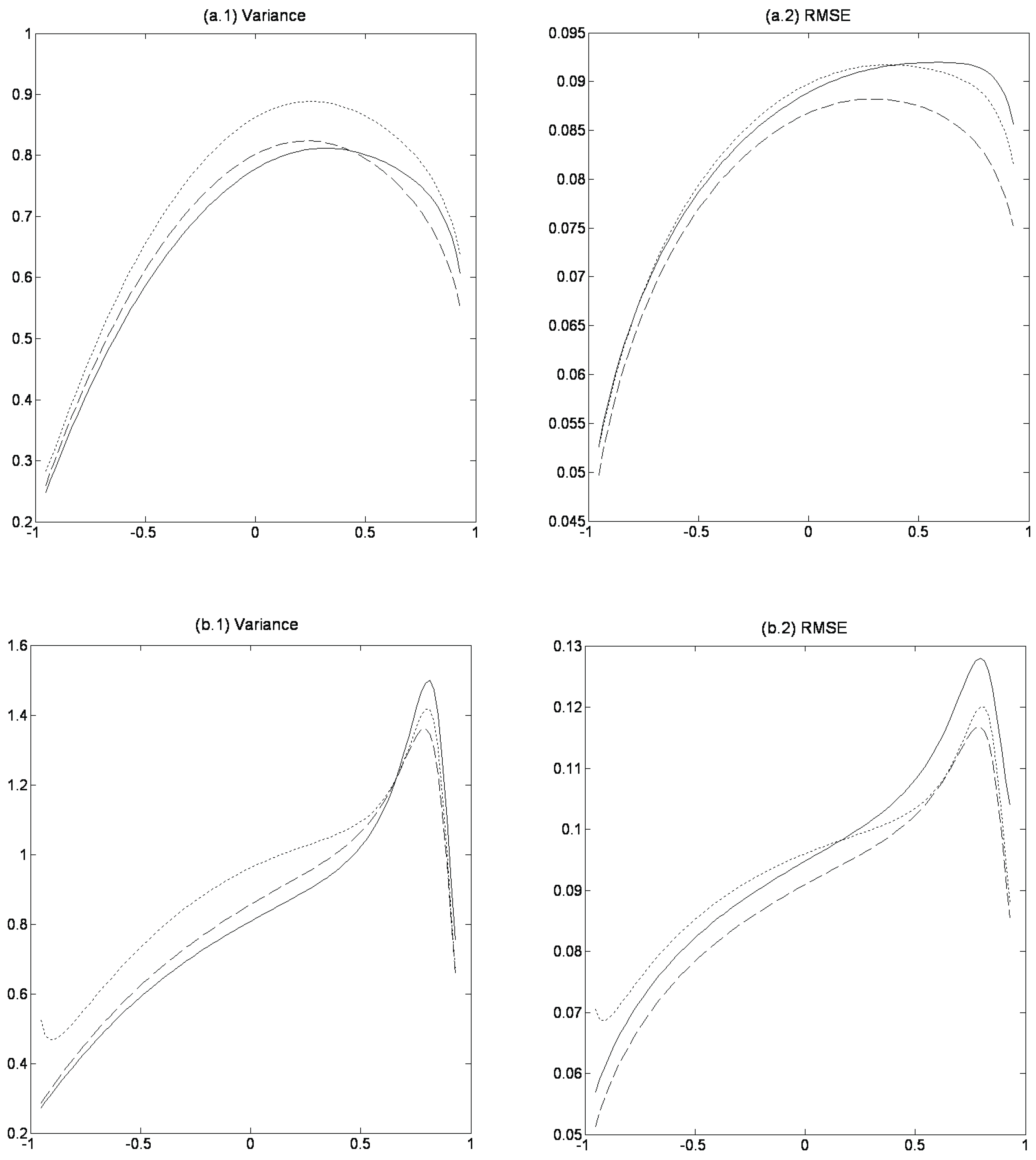
However, Table 2 also displays some interesting differences. The variances of the bias correction methods are now larger than that of OLS. This prompts the questions: What has caused this relative change in variances (Φ or ${\mathrm{\Omega }}_u$), and can the change imply a larger RMSE when correcting for bias than when not? To answer these questions, Figure 1 shows the variance of OLS, WLS, and ABF as a function of ${\mathrm{\Phi }}_{11}$ with the remaining data-generating parameters equal to those given in (11) and (12), respectively. The interval for ${\mathrm{\Phi }}_{11}$ is chosen to ensure stationarity. The variance is calculated as the average variance across the four slope coefficients based on 10,000 simulations with $T=100$.10 For the data-generating parameters given in (11), Panel (a.1) shows that for ${\mathrm{\Phi }}_{11}$ smaller (larger) than roughly $0.4$ the variance of OLS is smaller (larger) than the variance of ABF. Panel (b.1) shows the corresponding results for the data-generating parameters given in (12), i.e. the only differences between the two panels is ${\mathrm{\Omega }}_u$. We see a similar result as in Panel (a.1), but now ${\mathrm{\Phi }}_{11}$ has to be smaller (larger) than roughly 0.65 for the variance of OLS to be smaller (larger) than the variance of ABF.

Table 2. Bias-correction in a stationary but persistent VAR(1) model. The results in this table are based on 10,000 simulations from the VAR(1) model given in (12). See also the caption to Table 1.

		Mean Slope Coefficients
		${\mathrm{\Phi }}_{11}$	${\mathrm{\Phi }}_{12}$	${\mathrm{\Phi }}_{21}$	${\mathrm{\Phi }}_{22}$	Bias${}^2$	Variance	RMSE	#NS
$T=50$	OLS	0.1290	0.1841	0.0534	0.7509	0.4974	1.9419	0.1561	4
	WLS	0.0911	0.1222	0.1056	0.8260	0.0295	2.1234	0.1446	63
	ABF	0.1016	0.1162	0.0961	0.8312	0.0158	2.1547	0.1463	621
	BOOT	0.1015	0.1107	0.0970	0.8383	0.0065	2.1544	0.1460	669
$T=100$	OLS	0.1141	0.1400	0.0776	0.8030	0.1126	0.8412	0.0969	0
	WLS	0.0839	0.0979	0.1168	0.8536	0.0140	1.0066	0.0982	0
	ABF	0.0996	0.1038	0.1002	0.8457	0.0008	0.8978	0.0932	14
	BOOT	0.0993	0.1018	0.1006	0.8482	0.0002	0.9002	0.0933	7
$T=200$	OLS	0.1079	0.1195	0.0878	0.8270	0.0280	0.3925	0.0638	0
	WLS	0.0826	0.0877	0.1194	0.8650	0.0264	0.5321	0.0725	0
	ABF	0.1006	0.1012	0.0991	0.8486	0.0001	0.4049	0.0622	0
	BOOT	0.1005	0.1005	0.0994	0.8494	0.0000	0.4057	0.0622	0
$T=500$	OLS	0.1024	0.1070	0.0957	0.8414	0.0037	0.1506	0.0382	0
	WLS	0.0844	0.0860	0.1177	0.8664	0.0256	0.2372	0.0500	0
	ABF	0.0995	0.0996	0.1003	0.8501	0.0000	0.1524	0.0378	0
	BOOT	0.0995	0.0995	0.1003	0.8503	0.0000	0.1526	0.0378	0

Table 2. Bias-correction in a stationary but persistent VAR(1) model. The results in this table are based on 10,000 simulations from the VAR(1) model given in (12). See also the caption to Table 1.

		Mean Slope Coefficients
		${\mathrm{\Phi }}_{11}$	${\mathrm{\Phi }}_{12}$	${\mathrm{\Phi }}_{21}$	${\mathrm{\Phi }}_{22}$	Bias${}^2$	Variance	RMSE	#NS
$T=50$	OLS	0.1290	0.1841	0.0534	0.7509	0.4974	1.9419	0.1561	4
	WLS	0.0911	0.1222	0.1056	0.8260	0.0295	2.1234	0.1446	63
	ABF	0.1016	0.1162	0.0961	0.8312	0.0158	2.1547	0.1463	621
	BOOT	0.1015	0.1107	0.0970	0.8383	0.0065	2.1544	0.1460	669
$T=100$	OLS	0.1141	0.1400	0.0776	0.8030	0.1126	0.8412	0.0969	0
	WLS	0.0839	0.0979	0.1168	0.8536	0.0140	1.0066	0.0982	0
	ABF	0.0996	0.1038	0.1002	0.8457	0.0008	0.8978	0.0932	14
	BOOT	0.0993	0.1018	0.1006	0.8482	0.0002	0.9002	0.0933	7
$T=200$	OLS	0.1079	0.1195	0.0878	0.8270	0.0280	0.3925	0.0638	0
	WLS	0.0826	0.0877	0.1194	0.8650	0.0264	0.5321	0.0725	0
	ABF	0.1006	0.1012	0.0991	0.8486	0.0001	0.4049	0.0622	0
	BOOT	0.1005	0.1005	0.0994	0.8494	0.0000	0.4057	0.0622	0
$T=500$	OLS	0.1024	0.1070	0.0957	0.8414	0.0037	0.1506	0.0382	0
	WLS	0.0844	0.0860	0.1177	0.8664	0.0256	0.2372	0.0500	0
	ABF	0.0995	0.0996	0.1003	0.8501	0.0000	0.1524	0.0378	0
	BOOT	0.0995	0.0995	0.1003	0.8503	0.0000	0.1526	0.0378	0

Hence, the relative size of the variances for OLS and ABF depends on both Φ and ${\mathrm{\Omega }}_u,$ but in general, in highly persistent processes ABF has a lower variance than OLS. Panels (a.2) and (b.2) show that the RMSE for ABF remains below that of OLS for all values of ${\mathrm{\Phi }}_{11}$. Hence, despite a smaller variance for certain values of ${\mathrm{\Phi }}_{11}$, the larger bias using OLS results in a higher RMSE than in the case of ABF. This result does, however, not always hold. Table 3 reports the simulation results for the much less persistent VAR(1) model

$$\theta =\left[\begin{array}{c}0\\ 0\end{array}\right],\mathrm{ }\mathrm{\Phi }=\left[\begin{array}{cc}0.20& 0.10\\ 0.10& 0.25\end{array}\right],\mathrm{ }{\mathrm{\Omega }}_u=\left[\begin{array}{cc}2& 1\\ 1& 2\end{array}\right],\mathrm{ }$$

(13)

where the eigenvalues of Φ are 0.122 and 0.328. In contrast to the data-generating processes in (11) and (12) both variables now display little persistence. Although OLS in this case still yields somewhat biased estimates and WLS, ABF, and BOOT all reduce the bias, OLS has the lowest RMSE. This is due to a much lower variance for OLS than for the alternative estimator, WLS, and the two bias-correction methods, ABF and BOOT. The overall conclusion from Table 3 is that estimating even highly stationary VAR models using OLS provides biased estimates, which suggests the use of WLS, ABF, or BOOT if bias is of primary concern, while OLS is preferable if both bias and variance are important.

Table 3. Bias-correction in a stationary VAR(1) model. The results in this table are based on 10,000 simulations from the VAR(1) model given in (13). See also the caption to Table 1.

		Mean Slope Coefficients
		${\mathrm{\Phi }}_{11}$	${\mathrm{\Phi }}_{12}$	${\mathrm{\Phi }}_{21}$	${\mathrm{\Phi }}_{22}$	Bias${}^2$	Variance	RMSE	#NS
$T=50$	OLS	0.1627	0.0932	0.0964	0.2073	0.0819	2.8504	0.1712	0
	WLS	0.1850	0.0959	0.0980	0.2307	0.0155	2.9535	0.1723	0
	ABF	0.1949	0.0985	0.0988	0.2427	0.0021	2.9530	0.1719	0
	BOOT	0.1953	0.0986	0.0988	0.2432	0.0018	2.9550	0.1719	0
$T=100$	OLS	0.1803	0.0973	0.0983	0.2295	0.0204	1.3280	0.1161	0
	WLS	0.1919	0.0993	0.0992	0.2424	0.0031	1.3599	0.1167	0
	ABF	0.1974	0.1000	0.0995	0.2483	0.0002	1.3528	0.1163	0
	BOOT	0.1976	0.1000	0.0995	0.2484	0.0002	1.3546	0.1164	0
$T=200$	OLS	0.1912	0.0985	0.0992	0.2403	0.0044	0.6522	0.0810	0
	WLS	0.1971	0.0997	0.0997	0.2470	0.0004	0.6627	0.0814	0
	ABF	0.2000	0.0999	0.0998	0.2500	0.0000	0.6580	0.0811	0
	BOOT	0.2001	0.0999	0.0998	0.2500	0.0000	0.6587	0.0812	0
$T=500$	OLS	0.1962	0.0996	0.0998	0.2462	0.0007	0.2545	0.0505	0
	WLS	0.1986	0.1000	0.1000	0.2489	0.0001	0.2558	0.0506	0
	ABF	0.1998	0.1001	0.1000	0.2501	0.0000	0.2554	0.0505	0
	BOOT	0.1999	0.1001	0.1000	0.2502	0.0000	0.2555	0.0505	0

Table 3. Bias-correction in a stationary VAR(1) model. The results in this table are based on 10,000 simulations from the VAR(1) model given in (13). See also the caption to Table 1.

		Mean Slope Coefficients
		${\mathrm{\Phi }}_{11}$	${\mathrm{\Phi }}_{12}$	${\mathrm{\Phi }}_{21}$	${\mathrm{\Phi }}_{22}$	Bias${}^2$	Variance	RMSE	#NS
$T=50$	OLS	0.1627	0.0932	0.0964	0.2073	0.0819	2.8504	0.1712	0
	WLS	0.1850	0.0959	0.0980	0.2307	0.0155	2.9535	0.1723	0
	ABF	0.1949	0.0985	0.0988	0.2427	0.0021	2.9530	0.1719	0
	BOOT	0.1953	0.0986	0.0988	0.2432	0.0018	2.9550	0.1719	0
$T=100$	OLS	0.1803	0.0973	0.0983	0.2295	0.0204	1.3280	0.1161	0
	WLS	0.1919	0.0993	0.0992	0.2424	0.0031	1.3599	0.1167	0
	ABF	0.1974	0.1000	0.0995	0.2483	0.0002	1.3528	0.1163	0
	BOOT	0.1976	0.1000	0.0995	0.2484	0.0002	1.3546	0.1164	0
$T=200$	OLS	0.1912	0.0985	0.0992	0.2403	0.0044	0.6522	0.0810	0
	WLS	0.1971	0.0997	0.0997	0.2470	0.0004	0.6627	0.0814	0
	ABF	0.2000	0.0999	0.0998	0.2500	0.0000	0.6580	0.0811	0
	BOOT	0.2001	0.0999	0.0998	0.2500	0.0000	0.6587	0.0812	0
$T=500$	OLS	0.1962	0.0996	0.0998	0.2462	0.0007	0.2545	0.0505	0
	WLS	0.1986	0.1000	0.1000	0.2489	0.0001	0.2558	0.0506	0
	ABF	0.1998	0.1001	0.1000	0.2501	0.0000	0.2554	0.0505	0
	BOOT	0.1999	0.1001	0.1000	0.2502	0.0000	0.2555	0.0505	0

Figure 1(a.1) shows that for all values of ${\mathrm{\Phi }}_{11}$ WLS yields a larger variance than both OLS and ABF, and in Figure 1(b.1) this is the case for ${\mathrm{\Phi }}_{11}$ smaller than roughly 0.65. The bias-reduction from WLS compared to OLS only offsets this larger variance for ${\mathrm{\Phi }}_{11}$ larger than roughly $0.4$ and 0.2, respectively, cf. Figure 1(a.2) and (b.2). However, WLS is derived under the assumption of fixed initial values. 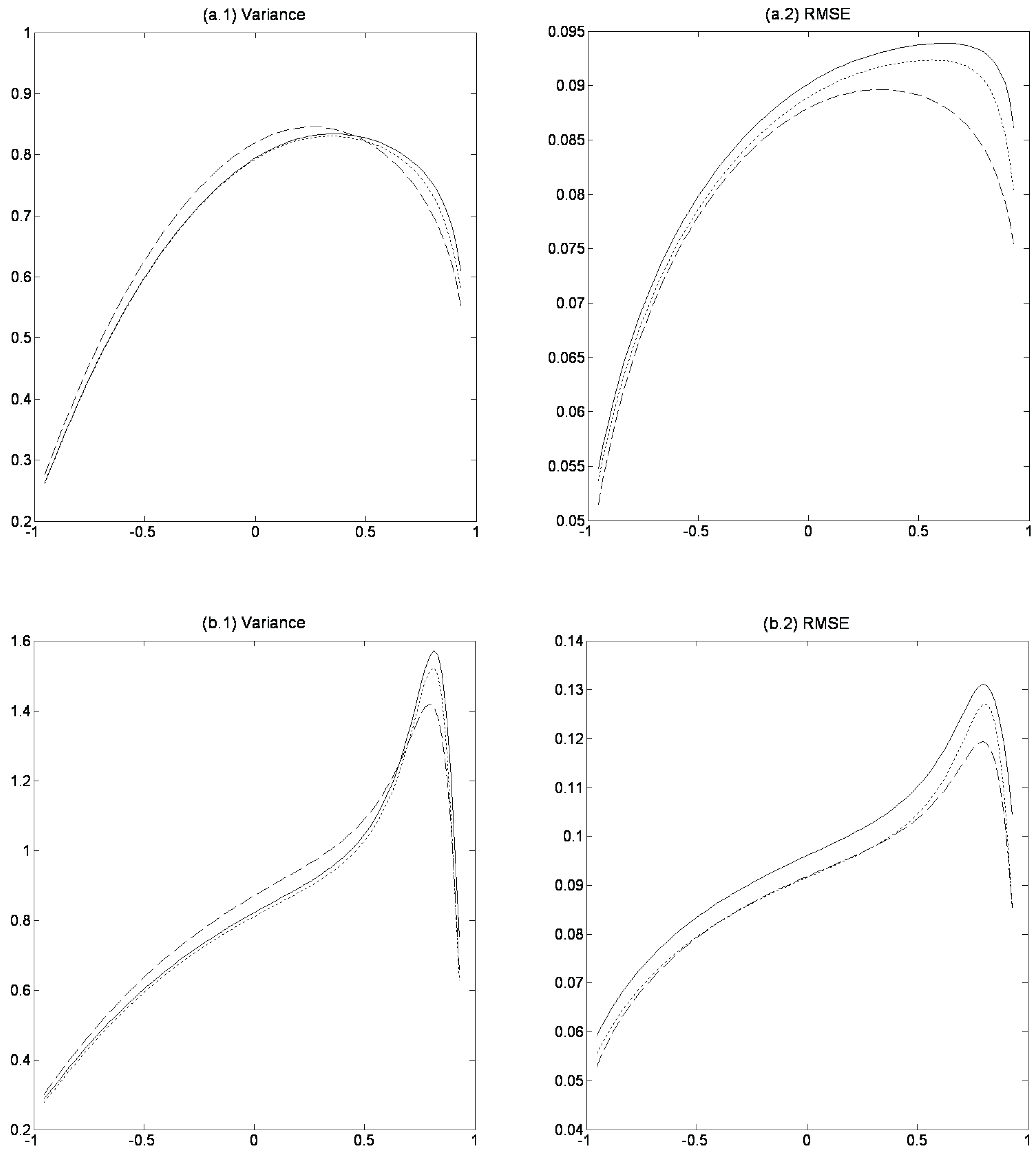Figure 2 shows results corresponding to those in Figure 1 but now with fixed initial values, which provides a more fair comparison of WLS to OLS and ABF. Comparing the two figures we see that fixed initial values clearly improve the finite-sample properties of WLS. The variance of WLS is now always smaller than or roughly equal to that of OLS, which together with a smaller bias implies that RMSE is lower for WLS than for OLS. However, despite better finite-sample properties under fixed initial values, WLS still does not yield a lower RMSE than ABF. Note, the relative findings on OLS and ABF are unaffected by the choice of random or fixed initial values.

Figure 1. Variance and RMSE with random initial value. The figure shows the variance and RMSE in the VAR(1) slope coefficients based on 10,000 simulations as a function of ${\mathrm{\Phi }}_{11}$ for OLS (solid line), WLS (dotted line), and ABF (dashed line). The remaining data-generating parameters are in Panel a given in (11) and in Panel b given in (12). The sample size is 100. The variance and RMSE are reported as the average across the four slope coefficients. The variance is multiplied by 100.

Figure 1. Variance and RMSE with random initial value. The figure shows the variance and RMSE in the VAR(1) slope coefficients based on 10,000 simulations as a function of ${\mathrm{\Phi }}_{11}$ for OLS (solid line), WLS (dotted line), and ABF (dashed line). The remaining data-generating parameters are in Panel a given in (11) and in Panel b given in (12). The sample size is 100. The variance and RMSE are reported as the average across the four slope coefficients. The variance is multiplied by 100.

Figure 2. Variance and RMSE with fixed initial value. See caption to Figure 1.

Figure 2. Variance and RMSE with fixed initial value. See caption to Figure 1.

3.2. Iterating and Inverting the Analytical Bias Formula

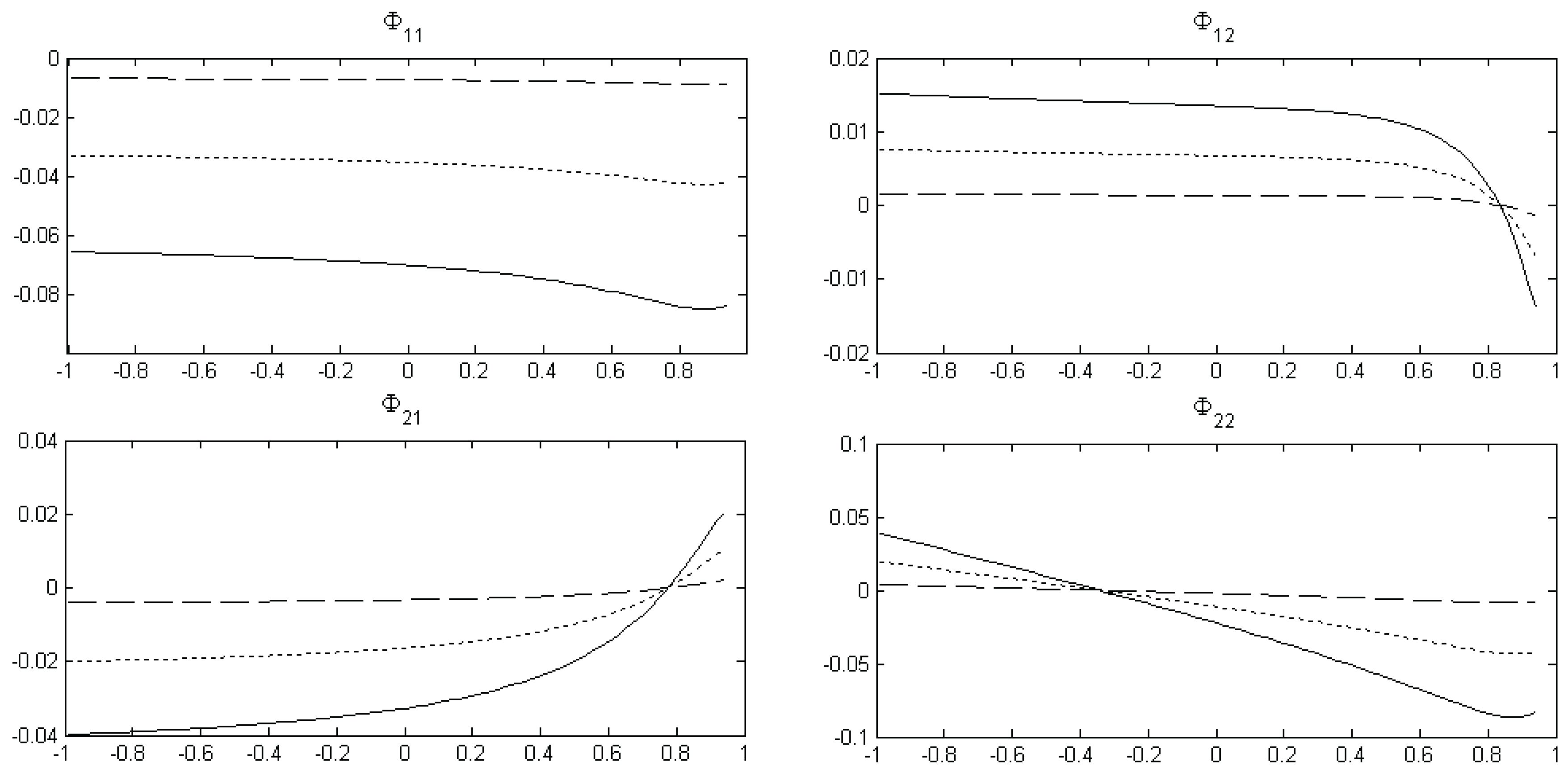
The use of an iterative scheme in the analytical bias formula is only relevant if the bias varies as a function of Φ.11 Figure 3 shows the bias as a function of ${\mathrm{\Phi }}_{22}$ in a bivariate VAR(1) system with the remaining data-generating parameters equal to those given in (11). As expected the bias function varies most for small sample sizes, but even for $T=50$ the bias function for ${\mathrm{\Phi }}_{11}$ is relatively flat. For ${\mathrm{\Phi }}_{12}$ and ${\mathrm{\Phi }}_{21}$ the bias function is relatively steep when the sample size is small and the second variable in the system is fairly persistent. For ${\mathrm{\Phi }}_{22}$ the bias function is mainly downward sloping. 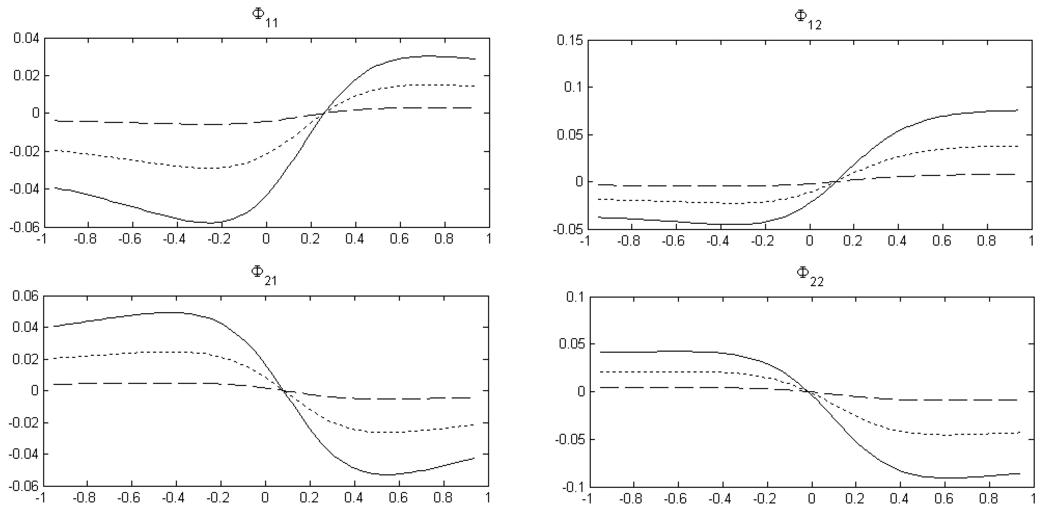Overall, Figure 3 suggests that the use of an iterative scheme could potentially be useful if the sample size is small, while for larger sample sizes the gain appears to be limited. Of course these plots depend on Φ and the correlation between the innovations. To illustrate the effect of changing Φ and ${\mathrm{\Omega }}_u$, Figure 4 shows the bias also as a function of ${\mathrm{\Phi }}_{22}$ but with the remaining data-generating parameters equal to those given in (12). Comparing Figure 4 with Figure 3 it is clear that the bias functions are quite different. For example, all the bias functions are now very flat when the second variable is highly persistent, which suggests a limited effect of using an iterative scheme when the data-generating process is given by (12).

Figure 3. Bias functions. The figure shows the least squares bias in the VAR(1) slope coefficients as a function of ${\mathrm{\Phi }}_{22}$ with the remaining data-generating parameters given in (11) for T = 50 (solid line), T = 100 (dotted line), and T = 500 (dashed line). The bias functions are calculated using the analytical bias formula (7).

Figure 3. Bias functions. The figure shows the least squares bias in the VAR(1) slope coefficients as a function of ${\mathrm{\Phi }}_{22}$ with the remaining data-generating parameters given in (11) for T = 50 (solid line), T = 100 (dotted line), and T = 500 (dashed line). The bias functions are calculated using the analytical bias formula (7).

Figure 4. Bias functions. The figure shows the least squares bias in the VAR(1) slope coefficients as a function of ${\mathrm{\Phi }}_{22}$ with the remaining data-generating parameters given in (12) for T = 50 (solid line), T = 100 (dotted line), and T = 500 (dashed line). The bias functions are calculated using the analytical bias formula (7).

Figure 4. Bias functions. The figure shows the least squares bias in the VAR(1) slope coefficients as a function of ${\mathrm{\Phi }}_{22}$ with the remaining data-generating parameters given in (12) for T = 50 (solid line), T = 100 (dotted line), and T = 500 (dashed line). The bias functions are calculated using the analytical bias formula (7).

Table 4 shows simulation results for the iterative scheme using the data-generating processes in (11) and (12), respectively. The convergence criteria used in the iterative scheme is that the maximum difference across the slope coefficients between two consecutive iterations must be smaller than 10${}^{-4}$.12 We calculate ${\widehat{\mathrm{\Omega }}}_x$ as $vec({\widehat{\mathrm{\Omega }}}_x)={(I_{k\times k}-\widehat{\mathrm{\Phi }}\otimes \widehat{\mathrm{\Phi }})}^{-1}vec({\widehat{\mathrm{\Omega }}}_u)$, which implies that we in applying the iterative scheme for the analytical bias formula also reestimate ${\mathrm{\Omega }}_x$ for each iteration based on the ’new’ estimates of Φ and ${\mathrm{\Omega }}_u$.13 For ease of comparison, Table 4 also contains the results based on the simple ‘plug-in’ approach as reported in Table 1 and Table 2.

Regarding WLS, Table 4 shows that with the data-generating process given in (11) iteration reduces the bias but increases the variance. Only for $T=50$ is the bias reduction of a sufficient magnitude to offset the increase in variance implying a decrease in RMSE. For $T\ge 100$ RMSE increases when iterating on the WLS estimator.14 For the data-generating process given in (12) the results for WLS are quite different. Using an iterative scheme, bias is now larger than for the ‘plug-in’ approach when $T\ge 100$. Also, bias increases as a function of the sample size up to $T=200$. However, due to a large decrease in variance, RMSE still decreases as the sample size increases.

Table 4. Bias-correction using an iterative scheme. The results in Panel A are based on 10,000 simulations from the VAR(1) model given in (11). The results in Panel B are based on the model given in (12). WLS${}^{*}$ and ABF${}^{*}$ give the results when using an iterative scheme for WLS and ABF, respectively. ABF${}^{**}$ gives the results when inverting the analytical bias formula to obtain an estimate of the bias. See also the caption to Table 1.

		Panel A				Panel B
		Bias${}^2$	Variance	RMSE	#NS	Bias${}^2$	Variance	RMSE	#NS
$T=50$	WLS	0.1606	1.9135	0.1438	198	0.0295	2.1234	0.1446	63
	WLS${}^{*}$	0.0511	1.9831	0.1423	612	0.0104	2.4418	0.1531	182
	ABF	0.0382	1.7520	0.1336	1613	0.0151	2.1350	0.1456	446
	ABF${}^{*}$	0.0284	1.7090	0.1317	1652	0.0082	2.1452	0.1456	535
	ABF${}^{**}$	0.0409	1.5396	0.1254	5912	0.1897	2.1390	0.1514	3054
$T=100$	WLS	0.0229	0.7549	0.0880	21	0.0109	1.0095	0.0984	2
	WLS${}^{*}$	0.0015	0.8646	0.0928	102	0.0284	1.1795	0.1062	6
	ABF	0.0025	0.6821	0.0826	307	0.0016	0.8992	0.0934	6
	ABF${}^{*}$	0.0018	0.6750	0.0821	312	0.0009	0.9011	0.0934	7
	ABF${}^{**}$	0.0444	0.6205	0.0813	2847	0.0796	0.9471	0.1003	337
$T=200$	WLS	0.0021	0.3471	0.0590	0	0.0264	0.5237	0.0720	0
	WLS${}^{*}$	0.0019	0.4428	0.0664	3	0.0581	0.6566	0.0818	0
	ABF	0.0001	0.3004	0.0547	1	0.0001	0.4059	0.0621	0
	ABF${}^{*}$	0.0001	0.2995	0.0546	1	0.0001	0.4062	0.0622	0
	ABF${}^{**}$	0.0198	0.2854	0.0551	164	0.0230	0.4184	0.0652	0
$T=500$	WLS	0.0004	0.1322	0.0363	0	0.0227	0.2367	0.0496	0
	WLS${}^{*}$	0.0030	0.1942	0.0442	0	0.0511	0.3338	0.0607	0
	ABF	0.0000	0.1091	0.0329	0	0.0000	0.1550	0.0381	0
	ABF${}^{*}$	0.0000	0.1090	0.0329	0	0.0000	0.1550	0.0381	0
	ABF${}^{**}$	0.0035	0.1067	0.0331	0	0.0036	0.1568	0.0389	0

Table 4. Bias-correction using an iterative scheme. The results in Panel A are based on 10,000 simulations from the VAR(1) model given in (11). The results in Panel B are based on the model given in (12). WLS${}^{*}$ and ABF${}^{*}$ give the results when using an iterative scheme for WLS and ABF, respectively. ABF${}^{**}$ gives the results when inverting the analytical bias formula to obtain an estimate of the bias. See also the caption to Table 1.

		Panel A				Panel B
		Bias${}^2$	Variance	RMSE	#NS	Bias${}^2$	Variance	RMSE	#NS
$T=50$	WLS	0.1606	1.9135	0.1438	198	0.0295	2.1234	0.1446	63
	WLS${}^{*}$	0.0511	1.9831	0.1423	612	0.0104	2.4418	0.1531	182
	ABF	0.0382	1.7520	0.1336	1613	0.0151	2.1350	0.1456	446
	ABF${}^{*}$	0.0284	1.7090	0.1317	1652	0.0082	2.1452	0.1456	535
	ABF${}^{**}$	0.0409	1.5396	0.1254	5912	0.1897	2.1390	0.1514	3054
$T=100$	WLS	0.0229	0.7549	0.0880	21	0.0109	1.0095	0.0984	2
	WLS${}^{*}$	0.0015	0.8646	0.0928	102	0.0284	1.1795	0.1062	6
	ABF	0.0025	0.6821	0.0826	307	0.0016	0.8992	0.0934	6
	ABF${}^{*}$	0.0018	0.6750	0.0821	312	0.0009	0.9011	0.0934	7
	ABF${}^{**}$	0.0444	0.6205	0.0813	2847	0.0796	0.9471	0.1003	337
$T=200$	WLS	0.0021	0.3471	0.0590	0	0.0264	0.5237	0.0720	0
	WLS${}^{*}$	0.0019	0.4428	0.0664	3	0.0581	0.6566	0.0818	0
	ABF	0.0001	0.3004	0.0547	1	0.0001	0.4059	0.0621	0
	ABF${}^{*}$	0.0001	0.2995	0.0546	1	0.0001	0.4062	0.0622	0
	ABF${}^{**}$	0.0198	0.2854	0.0551	164	0.0230	0.4184	0.0652	0
$T=500$	WLS	0.0004	0.1322	0.0363	0	0.0227	0.2367	0.0496	0
	WLS${}^{*}$	0.0030	0.1942	0.0442	0	0.0511	0.3338	0.0607	0
	ABF	0.0000	0.1091	0.0329	0	0.0000	0.1550	0.0381	0
	ABF${}^{*}$	0.0000	0.1090	0.0329	0	0.0000	0.1550	0.0381	0
	ABF${}^{**}$	0.0035	0.1067	0.0331	0	0.0036	0.1568	0.0389	0

For the analytical bias formula iteration generally yields a small reduction in bias compared to the ‘plug-in’ approach, while the effect on variance depends on the data-generating process. For the process given in (11) variance decreases slightly when iterating, while there is a small increase for the process given in (12). Comparing the effect on RMSE from using an iterative scheme relative to the ‘plug-in’ approach, we only see a noticeable decrease for (11) with $T=50$. This result is consistent with the bias functions shown in Figure 3 and Figure 4, and suggests that iteration often has a limited effect.

Instead of iterating on the analytical bias formula, we can (conditional on $\widehat{\mathrm{\Phi }}$) use it to back out the ’true’ Φ (and thereby ${\mathrm{\Omega }}_u$ and ${\mathrm{\Omega }}_x$), which can then be inserted into the bias formula to obtain an estimate of the bias. Table 4 shows that this approach generally has a noticeably larger bias than both the ‘plug-in’ approach and the iterative scheme.15 The effect on the variance depends on the data-generating process. For the process given in (11) variance is lowest when inverting the bias formula resulting in a slightly lower RMSE compared to the other two approaches, while for (12) the variance and RMSE are both higher when inverting.

3.3. Bias-Correction in Nearly Non-Stationary Models

Although the true VAR system is stationary, we often face the risk of finding unit or explosive roots when estimating a persistent system based on a finite sample. In Table 1 for $T=50$ we found that in 25 out of 10,000 simulations, OLS yields a non-stationary system. When correcting for bias using either the analytical bias formula or a bootstrap procedure this number increases considerably. In this section we compare the finite-sample properties of OLS (both with and without bias-correction) to the Yule-Walker (YW) estimator, which is guaranteed to ensure a stationary system. We also analyze how Kilian’s [10] approach to ensure stationarity affects the finite-sample properties of the bias-correction methods.

Table 5 reports simulation results for the following VAR(1) model

$$\theta =\left[\begin{array}{c}0\\ 0\end{array}\right],\mathrm{ }\mathrm{\Phi }=\left[\begin{array}{cc}0.80& 0.10\\ 0.10& 0.94\end{array}\right],\mathrm{ }{\mathrm{\Omega }}_u=\left[\begin{array}{cc}2& 1\\ 1& 2\end{array}\right],\mathrm{ }$$

(14)

where the eigenvalues of Φ are 0.748 and 0.992. This VAR(1) model is also used in a simulation study by Amihud et al. [32] and is more persistent than the ones used in Table 1, Table 2, Table 3 and Table 4, which increases the risk of estimating a non-stationary model using OLS and entering the non-stationary region of the parameter space when correcting for bias. Panel A shows the finite-sample properties of the OLS and YW estimators. Panel B reports the results when using Kilian’s approach to ensure stationarity when correcting for bias using the analytical bias formulas (6) and (8) and bootstrapping (only OLS), while Panel C shows the corresponding results without applying Kilian’s approach. The sample size is 100.16

From Panel A it is clear that YW has a much larger bias than OLS. This is also the case for the variance and, hence, the RMSE for YW is larger than for OLS. However, in contrast to OLS, YW always results in a stationary system, which implies that it is always possible to adjust for bias using the analytical bias formula. In Table 5, OLS yields a non-stationary model in 250 out of 10,000 simulations. The question now is if using the analytical bias formula for YW yields similar finite-sample properties as in the case of OLS? Panel B (where the procedure by Kilian [10] is applied) shows that this is not the case. YW still has a larger bias than OLS and the variance is more that three times as large. Comparing the results for YW with and without bias correction we see that the bias is clearly reduced by applying the analytical bias formula, but the variance also more than doubles. It is also worth noting that in 7,055 out of 10,000 simulations the system ends up in the non-stationary region when correcting YW for bias compared to only 3,567 for OLS.17

Table 5. Bias-correction in a nearly non-stationary VAR(1) model. The results in this table are based on 10,000 simulations from the VAR(1) model given in (14). The sample size is 100. Panel A shows the results from estimating the VAR(1) model using ordinary least squares (OLS) and Yule-Walker (YW). Panel B and C show the results when adjusting the ordinary least squares estimate for bias using the analytical bias formula (7) (ABF) and bootstrapping (BOOT), and when adjusting the Yule-Walker estimate for bias using the analytical bias formula (8). In Panel B (in contrast to Panel C) the correction by Kilian (1998a) to ensure a stationary VAR system is applied. See also the caption to Table 1.

	Mean Slope Coefficients
	${\mathrm{\Phi }}_{11}$	${\mathrm{\Phi }}_{12}$	${\mathrm{\Phi }}_{21}$	${\mathrm{\Phi }}_{22}$	Bias${}^2$	Variance	RMSE	#NS
Panel A
OLS	0.7508	0.0885	0.1032	0.8890	0.1290	0.6056	0.0844	250
YW	0.6567	-0.0649	0.1542	0.9582	1.2748	0.6578	0.1284	0
Panel B
ABF (OLS)	0.7813	0.0943	0.0968	0.9217	0.0182	0.5585	0.0745	3567
ABF (YW)	0.7829	0.0922	0.1105	0.9036	0.0448	1.7573	0.1297	7055
BOOT	0.7823	0.0951	0.0986	0.9234	0.0153	0.5709	0.0750	4266
Panel C
ABF (OLS)	0.7872	0.0951	0.0958	0.9276	0.0089	0.5599	0.0742	3567
ABF (YW)	0.8778	0.1465	0.1522	0.9398	0.2734	2$\times {10}^2$	1.4960	7055
BOOT	0.7904	0.0962	0.0980	0.9311	0.0047	0.5785	0.0750	4266

Table 5. Bias-correction in a nearly non-stationary VAR(1) model. The results in this table are based on 10,000 simulations from the VAR(1) model given in (14). The sample size is 100. Panel A shows the results from estimating the VAR(1) model using ordinary least squares (OLS) and Yule-Walker (YW). Panel B and C show the results when adjusting the ordinary least squares estimate for bias using the analytical bias formula (7) (ABF) and bootstrapping (BOOT), and when adjusting the Yule-Walker estimate for bias using the analytical bias formula (8). In Panel B (in contrast to Panel C) the correction by Kilian (1998a) to ensure a stationary VAR system is applied. See also the caption to Table 1.

	Mean Slope Coefficients
	${\mathrm{\Phi }}_{11}$	${\mathrm{\Phi }}_{12}$	${\mathrm{\Phi }}_{21}$	${\mathrm{\Phi }}_{22}$	Bias${}^2$	Variance	RMSE	#NS
Panel A
OLS	0.7508	0.0885	0.1032	0.8890	0.1290	0.6056	0.0844	250
YW	0.6567	-0.0649	0.1542	0.9582	1.2748	0.6578	0.1284	0
Panel B
ABF (OLS)	0.7813	0.0943	0.0968	0.9217	0.0182	0.5585	0.0745	3567
ABF (YW)	0.7829	0.0922	0.1105	0.9036	0.0448	1.7573	0.1297	7055
BOOT	0.7823	0.0951	0.0986	0.9234	0.0153	0.5709	0.0750	4266
Panel C
ABF (OLS)	0.7872	0.0951	0.0958	0.9276	0.0089	0.5599	0.0742	3567
ABF (YW)	0.8778	0.1465	0.1522	0.9398	0.2734	2$\times {10}^2$	1.4960	7055
BOOT	0.7904	0.0962	0.0980	0.9311	0.0047	0.5785	0.0750	4266

Until now we have used the approach by Kilian [10] to ensure a stationary VAR system after correcting for bias. Based on the same 10,000 simulations as in Panel B, Panel C shows the finite-sample properties without applying Kilian’s approach. For OLS (using both the analytical bias formula and a bootstrap procedure) bias decreases and variance increases slightly when we allow the system to be non-stationary after bias-correction. This result is not surprising. The VAR system is highly persistent and very small changes in Φ can result in a non-stationary system, e.g., if ${\mathrm{\Phi }}_{22}$ is 0.95 instead of 0.94 the system has a unit root. Hence, when applying Kilian’s approach, we often force the estimated coefficients to be smaller than the true values. In contrast, when we allow the system to be non-stationary after bias-correction some of the estimated coefficients will be smaller than the true values and some will be larger and, hence, positive and negative bias will offset each other across the 10,000 simulations. Likewise, this will also imply that the variance is larger when we do not apply Kilian’s approach. However, comparing the results for OLS in Panel B and Panel C it is clear that these differences are very small, which implies that Kilian’s approach does not severely distort the finite-sample properties of the bias-correction methods; and this even though we apply the approach in roughly 4,000 out of 10,000 simulations. In contrast, for YW it turns out to be essential to use Kilian’s approach as seen from Panel C. Note also that allowing the system to be non-stationary (i.e. not applying Kilian’s approach) is not consistent with the fact that the analytical bias formula is derived under the assumption of stationarity.

3.4. Bias-Correction in Non-Stationary Models

One of the major advantages of the weighted least squares estimator by Chen and Deo [30] compared to the analytical bias formula is that it allows for unit roots. In Section 3.3 we simulated from a stationary but highly persistent VAR(1) model and we assumed that the researcher has a priori knowledge that the system is stationary and thus considered the approach by Kilian [10] to ensure stationarity when correcting for bias. As a robustness check we now simulate from a bivariate VAR(1) model with unit roots and we assume that the researcher acknowledges that the system might be non-stationary and thus does not want to force the system to be stationary. The analytical bias formula is derived under the assumption of stationarity so the analysis in this section is in principle invalid for ABF. However, similar to the analysis of the properties of WLS under random initial values, it is also of interest to examine the finite-sample properties of ABF in the non-stationary case. To our knowledge the asymptotic theory of the properties of the bootstrap bias-corrected estimator for unit root models has not yet been developed.

Table 6. Bias-correction in a bivariate VAR(1) model with one unit root. The results in this table are based on 10,000 simulations from the VAR(1) model given in (15). See also the caption to Table 1.

		Mean Slope Coefficients
		${\mathrm{\Phi }}_{11}$	${\mathrm{\Phi }}_{12}$	${\mathrm{\Phi }}_{21}$	${\mathrm{\Phi }}_{22}$	Bias${}^2$	Variance	RMSE	#NS
$T=50$	OLS	0.9694	-0.0505	0.1887	0.7900	0.5172	1.1895	0.1293	1153
	WLS	1.0227	-0.0597	0.1933	0.8048	0.2682	1.0373	0.1138	3067
	ABF	1.0168	-0.0319	0.1556	0.8583	0.1084	1.0444	0.1072	5830
	BOOT	1.0364	-0.0479	0.1584	0.8615	0.0489	1.1038	0.1071	6772
$T=100$	OLS	1.0235	-0.0521	0.1658	0.8451	0.1028	0.3098	0.0636	956
	WLS	1.0521	-0.0580	0.1677	0.8497	0.0503	0.2624	0.0557	2972
	ABF	1.0426	-0.0423	0.1441	0.8762	0.0274	0.2856	0.0558	5156
	BOOT	1.0553	-0.0514	0.1460	0.8776	0.0083	0.2892	0.0544	6083
$T=200$	OLS	1.0483	-0.0544	0.1534	0.8656	0.0222	0.0952	0.0340	754
	WLS	1.0626	-0.0581	0.1541	0.8668	0.0108	0.0832	0.0306	3113
	ABF	1.0560	-0.0501	0.1415	0.8791	0.0074	0.0928	0.0316	4819
	BOOT	1.0626	-0.0545	0.1422	0.8797	0.0023	0.0919	0.0306	5777
$T=500$	OLS	1.0625	-0.0580	0.1449	0.8754	0.0027	0.0258	0.0168	550
	WLS	1.0677	-0.0595	0.1451	0.8755	0.0013	0.0240	0.0158	3150
	ABF	1.0650	-0.0566	0.1401	0.8799	0.0009	0.0258	0.0163	4711
	BOOT	1.0674	-0.0583	0.1402	0.8801	0.0002	0.0254	0.0160	5558

Table 6. Bias-correction in a bivariate VAR(1) model with one unit root. The results in this table are based on 10,000 simulations from the VAR(1) model given in (15). See also the caption to Table 1.

		Mean Slope Coefficients
		${\mathrm{\Phi }}_{11}$	${\mathrm{\Phi }}_{12}$	${\mathrm{\Phi }}_{21}$	${\mathrm{\Phi }}_{22}$	Bias${}^2$	Variance	RMSE	#NS
$T=50$	OLS	0.9694	-0.0505	0.1887	0.7900	0.5172	1.1895	0.1293	1153
	WLS	1.0227	-0.0597	0.1933	0.8048	0.2682	1.0373	0.1138	3067
	ABF	1.0168	-0.0319	0.1556	0.8583	0.1084	1.0444	0.1072	5830
	BOOT	1.0364	-0.0479	0.1584	0.8615	0.0489	1.1038	0.1071	6772
$T=100$	OLS	1.0235	-0.0521	0.1658	0.8451	0.1028	0.3098	0.0636	956
	WLS	1.0521	-0.0580	0.1677	0.8497	0.0503	0.2624	0.0557	2972
	ABF	1.0426	-0.0423	0.1441	0.8762	0.0274	0.2856	0.0558	5156
	BOOT	1.0553	-0.0514	0.1460	0.8776	0.0083	0.2892	0.0544	6083
$T=200$	OLS	1.0483	-0.0544	0.1534	0.8656	0.0222	0.0952	0.0340	754
	WLS	1.0626	-0.0581	0.1541	0.8668	0.0108	0.0832	0.0306	3113
	ABF	1.0560	-0.0501	0.1415	0.8791	0.0074	0.0928	0.0316	4819
	BOOT	1.0626	-0.0545	0.1422	0.8797	0.0023	0.0919	0.0306	5777
$T=500$	OLS	1.0625	-0.0580	0.1449	0.8754	0.0027	0.0258	0.0168	550
	WLS	1.0677	-0.0595	0.1451	0.8755	0.0013	0.0240	0.0158	3150
	ABF	1.0650	-0.0566	0.1401	0.8799	0.0009	0.0258	0.0163	4711
	BOOT	1.0674	-0.0583	0.1402	0.8801	0.0002	0.0254	0.0160	5558

We consider two bivariate VAR(1) models. Table 6 reports results for the following system

$$\theta =\left[\begin{array}{c}0\\ 0\end{array}\right],\mathrm{ }\mathrm{\Phi }=\left[\begin{array}{cc}1.07& -0.06\\ 0.14& 0.88\end{array}\right],\mathrm{ }{\mathrm{\Omega }}_u=\left[\begin{array}{cc}1& 0.5\\ 0.5& 1\end{array}\right],\mathrm{ }$$

(15)

where the eigenvalues of Φ are 1 and 0.95, while Table 7 reports results for the system

$$\theta =\left[\begin{array}{c}0\\ 0\end{array}\right],\mathrm{ }\mathrm{\Phi }=\left[\begin{array}{cc}1.08& -0.04\\ 0.16& 0.92\end{array}\right],\mathrm{ }{\mathrm{\Omega }}_u=\left[\begin{array}{cc}1& 0.5\\ 0.5& 1\end{array}\right],\mathrm{ }$$

(16)

where both eigenvalues of Φ are 1. These two VAR(1) models are both used by Chen and Deo [30] in a simulation study of the finite-sample properties of WLS. Due to an infinite variance of $X_t$ in the presence of unit roots, in the simulation study initial values of $X_t$ are fixed and equal to 0 rather than random.

Table 6 and Table 7 both show that OLS delivers biased estimates and that WLS, ABF, and BOOT all reduce both bias and RMSE. Hence, even though ABF is derived under the assumption of stationarity, it still has better finite-sample properties than OLS. Comparing WLS, ABF, and BOOT in terms of bias we see that BOOT consistently delivers the smallest bias, irrespective of one or two unit roots. In contrast to the stationary case ABF performs noticeably worse than BOOT. It does, however, yield a smaller bias than WLS in the presence of one unit root, while the opposite is the case with two unit roots. With respect to variance WLS consistently performs best, especially so when there are two unit roots. Altogether these results imply that BOOT has the smallest RMSE when there is one unit root (and for small samples when there are two unit roots) while this is the case for WLS when there are two unit roots (and the sample size is not too small).

Table 7. Bias-correction in a bivariate VAR(1) model with two unit roots. The results in this table are based on 10,000 simulations from the VAR(1) model given (16). See also the caption to Table 1.

		Mean Slope Coefficients
		${\mathrm{\Phi }}_{11}$	${\mathrm{\Phi }}_{12}$	${\mathrm{\Phi }}_{21}$	${\mathrm{\Phi }}_{22}$	Bias${}^2$	Variance	RMSE	#NS
$T=50$	OLS	0.9575	-0.0075	0.1914	0.8665	0.4975	0.9676	0.1169	3390
	WLS	1.0220	-0.0247	0.2038	0.8749	0.1886	0.7893	0.0973	5748
	ABF	1.0064	0.0076	0.1630	0.9199	0.1922	0.8770	0.1021	7736
	BOOT	1.0413	-0.0259	0.1731	0.9082	0.0501	0.9029	0.0958	8377
$T=100$	OLS	1.0146	-0.0153	0.1704	0.9076	0.1289	0.2164	0.0549	4113
	WLS	1.0534	-0.0292	0.1779	0.9072	0.0327	0.1576	0.0423	6533
	ABF	1.0352	-0.0103	0.1566	0.9247	0.0731	0.2165	0.0522	8125
	BOOT	1.0620	-0.0311	0.1638	0.9184	0.0105	0.2063	0.0449	8561
$T=200$	OLS	1.0455	-0.0245	0.1634	0.9173	0.0362	0.0505	0.0269	4578
	WLS	1.0673	-0.0339	0.1670	0.9160	0.0066	0.0347	0.0195	6942
	ABF	1.0547	-0.0244	0.1585	0.9217	0.0223	0.0537	0.0261	8355
	BOOT	1.0710	-0.0352	0.1615	0.9195	0.0027	0.0487	0.0216	8671
$T=500$	OLS	1.0659	-0.0332	0.1605	0.9197	0.0061	0.0078	0.0106	4659
	WLS	1.0748	-0.0374	0.1614	0.9193	0.0009	0.0052	0.0074	7059
	ABF	1.0696	-0.0343	0.1595	0.9203	0.0035	0.0081	0.0100	8351
	BOOT	1.0764	-0.0381	0.1601	0.9200	0.0004	0.0075	0.0084	8653

Table 7. Bias-correction in a bivariate VAR(1) model with two unit roots. The results in this table are based on 10,000 simulations from the VAR(1) model given (16). See also the caption to Table 1.

		Mean Slope Coefficients
		${\mathrm{\Phi }}_{11}$	${\mathrm{\Phi }}_{12}$	${\mathrm{\Phi }}_{21}$	${\mathrm{\Phi }}_{22}$	Bias${}^2$	Variance	RMSE	#NS
$T=50$	OLS	0.9575	-0.0075	0.1914	0.8665	0.4975	0.9676	0.1169	3390
	WLS	1.0220	-0.0247	0.2038	0.8749	0.1886	0.7893	0.0973	5748
	ABF	1.0064	0.0076	0.1630	0.9199	0.1922	0.8770	0.1021	7736
	BOOT	1.0413	-0.0259	0.1731	0.9082	0.0501	0.9029	0.0958	8377
$T=100$	OLS	1.0146	-0.0153	0.1704	0.9076	0.1289	0.2164	0.0549	4113
	WLS	1.0534	-0.0292	0.1779	0.9072	0.0327	0.1576	0.0423	6533
	ABF	1.0352	-0.0103	0.1566	0.9247	0.0731	0.2165	0.0522	8125
	BOOT	1.0620	-0.0311	0.1638	0.9184	0.0105	0.2063	0.0449	8561
$T=200$	OLS	1.0455	-0.0245	0.1634	0.9173	0.0362	0.0505	0.0269	4578
	WLS	1.0673	-0.0339	0.1670	0.9160	0.0066	0.0347	0.0195	6942
	ABF	1.0547	-0.0244	0.1585	0.9217	0.0223	0.0537	0.0261	8355
	BOOT	1.0710	-0.0352	0.1615	0.9195	0.0027	0.0487	0.0216	8671
$T=500$	OLS	1.0659	-0.0332	0.1605	0.9197	0.0061	0.0078	0.0106	4659
	WLS	1.0748	-0.0374	0.1614	0.9193	0.0009	0.0052	0.0074	7059
	ABF	1.0696	-0.0343	0.1595	0.9203	0.0035	0.0081	0.0100	8351
	BOOT	1.0764	-0.0381	0.1601	0.9200	0.0004	0.0075	0.0084	8653

3.5. Bias-Correction When Data Are Skewed and Fat-Tailed

Until now we have generated data from a multivariate normal distribution. However, in many empirically relevant models the normality assumption often fails. The analytical bias formula is not derived under a normality assumption, but it is unclear how the finite-sample properties of bias-correction using ABF compare to those of bootstrapping if the data are, for example, very skewed and fat-tailed. Furthermore, researchers often use a parametric bootstrap based on a normal distribution instead of the usual residual-based bootstrap procedure. The obvious question here is: do we commit errors when using this parametric bootstrap approach when data are very skewed and fat-tailed? Also, WLS is derived under the assumption of normality. How does this estimator perform under skewed and fat-tailed data? In this section, we address these issues.

To obtain data that are skewed and have fat tails we use the data-generating parameters in (11) but follow Kilian [24] and make random draws for the innovations from a Student’s t-distribution with four degrees of freedom and a ${\chi }^2$-distribution with three degrees of freedom, respectively.18 Table 8 shows the results. For the bias-correction methods we use the approach by Kilian [10] to ensure stationarity. The sample size is 100.19

Table 8. Bias-correction in a VAR(1) model, skewed and fat-tailed innovations. The results in this table are based on 10,000 simulations from the VAR(1) model given in (11) but with innovations randomly drawn from Student’s t-distribution with four degrees of freedom (Panel A) and ${\chi }^2$-distribution with three degrees of freedom (Panel B). The sample size is 100. PARBOOT are bias-adjusted estimates from the bootstrap based on normally distributed innovations. See also the caption to Table 1.

	Mean Slope Coefficients
	${\mathrm{\Phi }}_{11}$	${\mathrm{\Phi }}_{12}$	${\mathrm{\Phi }}_{21}$	${\mathrm{\Phi }}_{22}$	Bias${}^2$	Variance	RMSE	#NS
Panel A
OLS	0.7541	0.0968	0.1008	0.8038	0.1063	0.7525	0.0925	2
WLS	0.7694	0.1035	0.1025	0.8244	0.0402	0.7554	0.0890	8
ABF	0.7921	0.0994	0.0983	0.8438	0.0026	0.7053	0.0840	489
BOOT	0.7933	0.1003	0.0993	0.8454	0.0017	0.7160	0.0846	525
PARBOOT	0.7938	0.1002	0.0993	0.8458	0.0014	0.7150	0.0845	542
Panel B
OLS	0.7590	0.1000	0.1029	0.8102	0.0817	0.6642	0.0861	2
WLS	0.8135	0.0885	0.0900	0.8578	0.0119	0.8981	0.0952	132
ABF	0.7941	0.0998	0.0991	0.8453	0.0015	0.6242	0.0790	307
BOOT	0.7989	0.1029	0.1010	0.8520	0.0004	0.6315	0.0794	450
PARBOOT	0.7994	0.1028	0.1009	0.8524	0.0004	0.6314	0.0794	451

Table 8. Bias-correction in a VAR(1) model, skewed and fat-tailed innovations. The results in this table are based on 10,000 simulations from the VAR(1) model given in (11) but with innovations randomly drawn from Student’s t-distribution with four degrees of freedom (Panel A) and ${\chi }^2$-distribution with three degrees of freedom (Panel B). The sample size is 100. PARBOOT are bias-adjusted estimates from the bootstrap based on normally distributed innovations. See also the caption to Table 1.

	Mean Slope Coefficients
	${\mathrm{\Phi }}_{11}$	${\mathrm{\Phi }}_{12}$	${\mathrm{\Phi }}_{21}$	${\mathrm{\Phi }}_{22}$	Bias${}^2$	Variance	RMSE	#NS
Panel A
OLS	0.7541	0.0968	0.1008	0.8038	0.1063	0.7525	0.0925	2
WLS	0.7694	0.1035	0.1025	0.8244	0.0402	0.7554	0.0890	8
ABF	0.7921	0.0994	0.0983	0.8438	0.0026	0.7053	0.0840	489
BOOT	0.7933	0.1003	0.0993	0.8454	0.0017	0.7160	0.0846	525
PARBOOT	0.7938	0.1002	0.0993	0.8458	0.0014	0.7150	0.0845	542
Panel B
OLS	0.7590	0.1000	0.1029	0.8102	0.0817	0.6642	0.0861	2
WLS	0.8135	0.0885	0.0900	0.8578	0.0119	0.8981	0.0952	132
ABF	0.7941	0.0998	0.0991	0.8453	0.0015	0.6242	0.0790	307
BOOT	0.7989	0.1029	0.1010	0.8520	0.0004	0.6315	0.0794	450
PARBOOT	0.7994	0.1028	0.1009	0.8524	0.0004	0.6314	0.0794	451

Overall, the results in Table 8 are in line with our previous findings for stationary models with random initial values, namely that OLS yields highly biased estimates, WLS is able to reduce this bias but at the cost of increased variance and the bias correction methods provide a large bias reduction compared to both OLS and WLS. Comparing ABF and BOOT, we see that similar to the results in Table 1, Table 2, Table 3 and Table 5, BOOT yields a slightly smaller bias than ABF and has a slightly higher variance.

In addition to the residual-based bootstrap approach, Table 8 also shows the results when applying a parametric bootstrap procedure based on an assumption of normally distributed data (PARBOOT). Given that the innovations are skewed and fat-tailed we could expect this approach to have inferior properties compared to both the residual-based bootstrap that directly takes into account the non-normality of the data, and the analytical bias formula that is derived without the assumption of normality. The results in Table 8 show that this is not the case. PARBOOT has both smaller bias and lower variance than BOOT. However, the differences are very small, and for all practical purposes the results in Table 8 suggest that the use of BOOT and PARBOOT will give similar results.

These results contrast those of Kilian [24] who examines the coverage accuracy of various methods for constructing confidence intervals for impulse responses when data are non-normally distributed. Two of the methods he considers are based on the analytical bias formula combined with a residual-based and a parametric (assuming Gaussianity) bootstrap procedure, respectively. Kilian finds that in terms of constructing confidence intervals for impulse responses the residual-based bootstrap procedure strictly dominates the parametric approach when data have fat tails and are skewed. In the present paper we consider parameter estimates and not confidence intervals, which inevitably depend on the entire distribution of innovations. Our results show that with respect to point estimates using an incorrect parametric bootstrap has no negative consequences, which lend support to the use of a parametric bootstrap procedure when data do not match the assumed distribution.

4. Summary of Results

The main results of our simulation study for VAR(1) models can be summarized as follows:

-

The analytical bias formula and the bootstrap approach both yield a very large reduction in bias compared to OLS, also when the model is highly stationary. For persistent but stationary models the variance of OLS is also higher than the variance of the bias-adjusted estimates. The less persistent the system is the better OLS performs in terms of variance, and for highly stationary models this results in OLS yielding the lowest mean squared error.

-

The properties in terms of both bias and variance of the analytical bias formula and the bootstrap approach are very similar in stationary models. In non-stationary models the analytical bias formula performs noticeably worse than bootstrapping.

-

The variance and thereby the mean squared error of WLS is highly sensitive to the initial value. The estimator has a lower mean squared error than OLS when the initial value is fixed while for random initial values it depends on the persistence of the system. In stationary models WLS has a larger bias than the analytical bias formula and bootstrapping, and irrespective of initial values also a higher mean squared error. In non-stationary models the lower variance can, however, in some cases lead to a lower mean squared error for WLS than for bootstrapping.

-

The iterative scheme, where bias-adjusted estimates repeatedly are inserted into the analytical bias formula, can for certain data-generating processes and very small sample sizes yield a minor improvement over the simple one-step ‘plug-in’ approach where biased least squares estimates are used in place of the true unknown parameters. For larger sample sizes there is no gain by iterating.

-

Even after correcting for bias the Yule-Walker estimator has very poor finite-sample properties compared to OLS.

-

Kilian’s [10] approach to ensure stationarity does not distort the finite-sample properties of the bias-adjusted estimates. The approach leads to a very small increase in bias but also a decrease in variance implying a basically unaffected mean squared error compared to the case where we allow the model to be non-stationary.

-

Despite skewed and fat-tailed data, with respect to point estimates parametric bootstrap bias-correction based on the normal distribution performs no worse than bootstrap bias-correction based on the non-normal residuals.