
Pair-Copula Constructions for Financial Applications: A Review

Department of Statistical Analysis, Image Analysis and Machine Learning, Norwegian Computing Center, N-0314 Oslo, Norway
Econometrics 2016, 4(4), 43; https://doi.org/10.3390/econometrics4040043
Submission received: 1 September 2016
/
Revised: 4 October 2016
/
Accepted: 18 October 2016
/
Published: 29 October 2016
(This article belongs to the Special Issue Recent Developments in Copula Models)
Abstract
:This survey reviews the large and growing literature on the use of pair-copula constructions (PCCs) in financial applications. Using a PCC, multivariate data that exhibit complex patterns of dependence can be modeled using bivariate copulae as simple building blocks. Hence, this model represents a very flexible way of constructing higher-dimensional copulae. In this paper, we survey inference methods and goodness-of-fit tests for such models, as well as empirical applications of the PCCs in finance and economics.
JEL Classification:
C13; C15; C51; C52; C53; C581. Introduction
Understanding and quantifying dependence is the core of all modeling efforts in financial econometrics. For modeling high dimensional data that exhibit non-linear dependence, a copula approach is often taken [1,2]. The concept of copulae was introduced already in 1959 by Sklar [3], but it was the seminal work of Embrechts et al. [4], introducing copulae to the field of financial risk management, that really lead to the incredible growth in papers published on this subject the last 15 years. From a practical point of view, the advantage of the copula-based approach is that the appropriate marginal distributions for the components of a multivariate system can be selected freely and then linked through a suitable copula. Hence, the dependence structure may be modeled independently of the marginal distributions.
For bivariate models, there exists a long and varied list of copula families; see, e.g., [1]. However, in higher dimensions, the selection of parametric copulae is still rather limited [5]. This has led to the development of hierarchical copula-based structures, of which the most promising is the pair-copula construction (PCC). This structure was originally proposed by Joe [6] and further explored and discussed by Bedford and Cooke [7,8] and Kurowicka and Cooke [9]. However, it was the work of Aas et al. [10], putting the PCC in an inferential context, that really spurred a surge in empirical applications of these constructions. During the last eight years, the pair-copula constructions have been applied within a number of different fields, including finance and insurance, genetics, marketing, health and hydrology. The focus of this survey is however on the financial applications.
In the sections that follow, we first give an overview of the pair-copula construction and its subclass, the regular vine. We then consider inference methods and goodness-of-fit tests for these models, and finally, we present a survey of some of the numerous applications of PCCs that have appeared in the economics and finance literature.
2. The Pair-Copula Construction and the Regular Vine
A PCC is a multivariate copula that is constructed from a set of bivariate ones, so-called pair-copulae. More specifically, the copula density is decomposed into a product of pair-copula densities. All of these bivariate copulae may be selected completely freely as the resulting structure is guaranteed to be a valid copula. Hence, PCCs are highly flexible and able to characterize a wide range of complex dependencies. Inference on PCCs is in general demanding, but the subclass of regular vines has many appealing computational properties and, hence, constitutes an exception in the inferential context.
The notion of regular vines (R-vines) was introduced by Bedford and Cooke [8], and described in more detail in [9]. It involves the specification of a sequence of trees, each edge of which corresponds to a pair-copula. These pair-copulae constitute the building blocks of the joint R-vine distribution. According to Definition 4.4 of [9], an R-vine on d variables consists of the trees (also denoted levels) . Let and be the sets of nodes and edges, respectively, in tree . Then, the following conditions are satisfied:
- Tree has nodes and edges .
- For , the nodes in tree are the edges in tree , i.e., .
- Proximity condition: if two edges in tree are to be joined as nodes in tree by an edge, they must share a common node in .
To build an R-vine with node set and edge set , one associates each edge e in with a bivariate copula . The nodes and are called the conditioned nodes, while is denoted the conditioning set and the union the constraint set. The copulae in tree have an empty conditioning set; in tree , these sets consist of one node, in tree of two nodes, and so on. Take, for instance, the edge joining and in the fourth tree of Figure 1, displaying a seven-dimensional R-vine tree specification. The conditioned nodes are 5 and 4; the conditioning set is ; and the constraint set is .
Let the random vector follow an R-vine distribution. Further, let denote the subvector of X determined by the indices constituting . Then, Theorem 4.2 in [9] states that the joint density of can be written as:
The right factor of the right-hand side of (1) is a product of bivariate copula densities and is called an R-vine copula. Note that the arguments of the pair-copulae are conditional distributions in all trees, but the first, where they are the univariate margins.
The key to the construction in (1) is that all copulae involved in the decomposition are bivariate and can belong to different families. There are no restrictions regarding the copula types that can be combined; the resulting structure is guaranteed to be valid anyhow. A further advantage with the R-vine copula is that the conditional distributions constituting the pair-copula arguments can be evaluated using a recursive formula derived in [6]:
Here, is a bivariate copula; is an arbitrary component of ; and denotes the vector excluding . By construction, R-vines have the important characteristic that the copulae in question always are present in the preceding trees of the structure, so that they are available without extra computations.
In order to find an expression for a general R-vine density, one needs an efficient way of storing the indices involved in the pair-copulae. One such approach was proposed by Morales-Napoles [11] and explored in more detail in [12]. It involves the specification of a lower triangular matrix whose diagonal entries are the nodes of the first tree. Further, each row of M from the bottom up represents a tree. The conditioned sets of a node are determined by a diagonal entry and the corresponding column entry of the row under consideration, while the conditioning set is given by the column entries below this row. The R-vine matrix corresponding to the R-vine in Figure 1 is:
To determine the edges in , we combine the numbers in the bottom row with the diagonal elements in the corresponding columns, i.e., the edges are (6,5), (7,5), (5,1), and so on. The edges of are given by the numbers in the second row from the bottom, associated with the diagonal elements, conditioning on the elements in the bottom row, namely (6,1|5), (7,1|5), etc. Proceeding like this, the only edge in is found by coupling the two upper elements in the leftmost column with the remaining five entries of the column as a conditioning set, i.e., (6,4|72,315).
Based on M, the R-vine density may be written as in [12]:
where the pair-copulae have arguments and . Corresponding copula types and parameters can conveniently be stored in matrices similar to M.
2.1. Simplifying Assumption
In their general form, PCCs can represent most continuous multivariate distributions. However, to keep them tractable for inference, the assumption that the pair-copulae are independent of the conditioning variables , except through the conditional distributions, is usually made, leading to the so-called simplified PCC.
Even though not all multivariate distributions can be represented by a simplified PCC, it may always be used as an approximation. The work in [13] shows that the approximation in fact may be a good one, even when the simplifying assumption is far from being fulfilled. This subject has also been investigated by Stöber et al. [14], Killiches et al. [15] and Spanhel and Kurz [16].
2.2. Canonical Vines and D-Vines
In financial applications, two special cases of regular vines have mainly been used. These are denoted canonical vines and D-vines, respectively [19]. Each model gives a specific way of decomposing the density. Figure 2 shows the specification corresponding to a five-dimensional D-vine. It consists of four trees . Tree has nodes and edges. Each edge corresponds to a pair-copula density, and the edge label corresponds to the subscript of the pair-copula density, e.g., edge corresponds to the copula density . The whole decomposition is defined by the edges and the marginal densities of each variable. The nodes in tree are only necessary for determining the labels of the edges in tree . As can be seen from Figure 2, two edges in , which become nodes in , are joined by an edge in only if these edges in share a common node.
The density corresponding to a D-vine may be written as:
where index j identifies the trees, while i runs over the edges in each tree. The D-vine in Figure 2 has density:
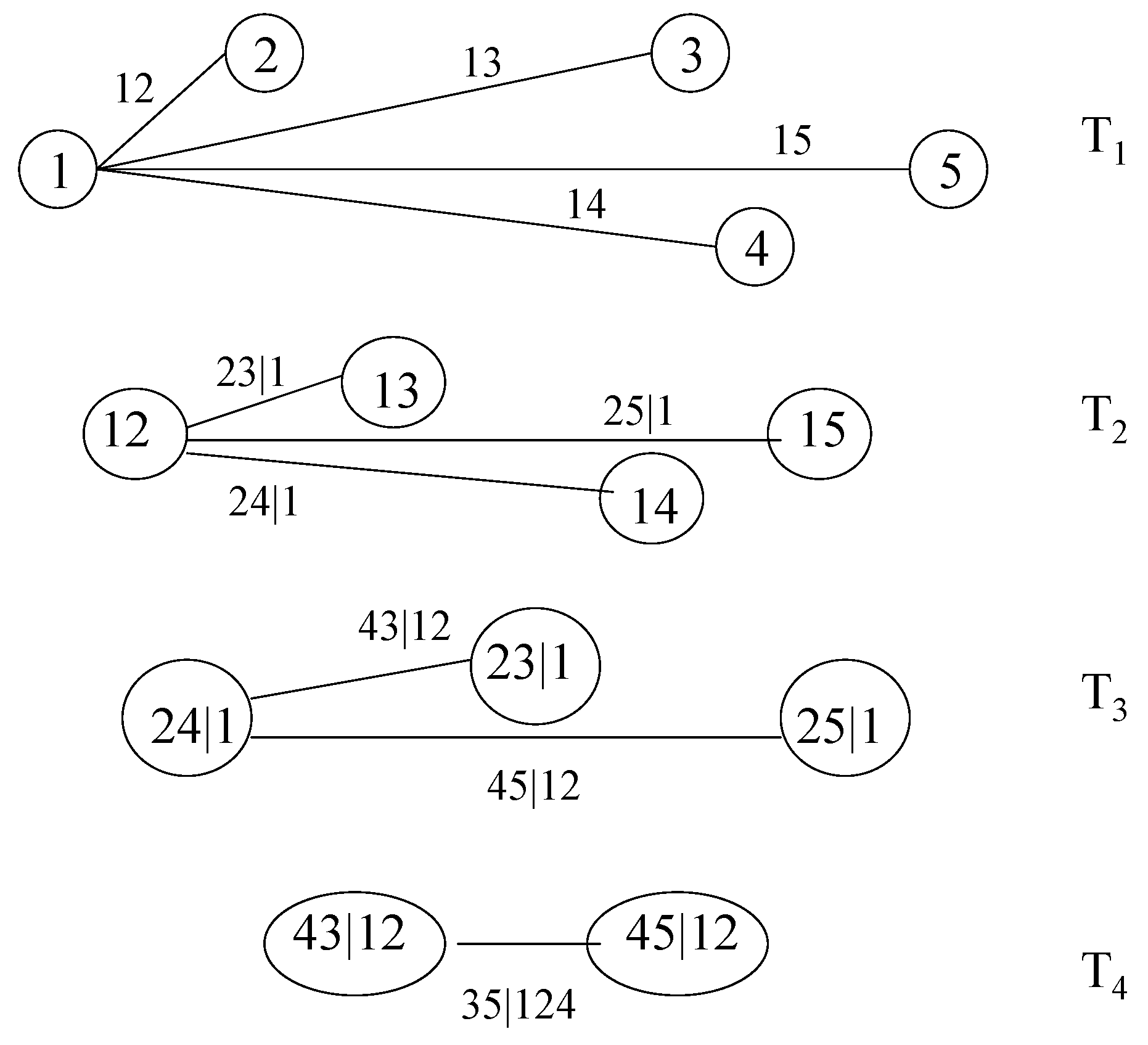
In a D-vine, no node in any tree is connected to more than two edges. In a canonical vine, each tree has a unique node that is connected to edges. Figure 3 shows a canonical vine with five variables. The n-dimensional density corresponding to a canonical vine is given by:
The canonical vine in Figure 3 has density:
Fitting a canonical vine might be advantageous when a particular variable is known to be a key variable that governs interactions in the dataset. In such a situation, one may decide to locate this variable at the root of the canonical vine, as we have done with Variable 1 in Figure 3.
2.3. Serial Dependence
To date, pair-copula constructions have been employed largely to account for cross-sectional dependence. Applications to serial dependence in time series and longitudinal data are rare. There are however some exceptions. The work in [20], studying intraday electricity load data, was the first to demonstrate the usefulness of serial PCCs. Later, Vaz de Melo Mendes and Accioly [21] have used canonical vines for modeling nonlinear temporal dependences of Brazilian series of realized volatilities, while in [22], the focus is on serial dependence in equity time series. Finally, Brechmann and Czado [23] recently introduced the so-called copula autoregressive model, COPAR, which allows for non-linear and non-symmetric modeling of both serial and between-series dependence.
3. Inference
Inference on R-vines consists of three tasks: (i) selecting the structure with all its trees; (ii) choosing a copula family for each of the pair-copulae; and (iii) estimating the parameters of each pair-copula. Ideally, Steps (i)–(ii) should be performed simultaneously. In practice, however, this is usually done stepwise. In what follows, we give a short review of the main approaches that have been used for each step. See [24,25] for more comprehensive surveys of the various model selection and estimation methods that have been used for regular vine copulae.
3.1. Structure Selection
The number of possible R-vines on d variables is [11]. Finding the globally-optimal R-vine structure for a given high-dimensional dataset is therefore unfeasible, but several useful strategies have been proposed. Since the first trees can be estimated with more precision, a natural strategy is to build the structure starting from the bottom, trying to maximize the dependence in the first trees. This strategy was originally proposed in [10] for canonical vines and D-vines and later extended to regular vines by Dißmann et al. [12]. The latter algorithm starts by finding the maximum spanning tree over the d nodes corresponding to the d variables using the well-known algorithm of [26]. This is a tree on all nodes that maximizes the sum of the weights of the edges, using measures of pairwise dependence as weights. The subsequent trees are built in a similar manner, under the additional restriction that the proximity condition must be fulfilled. This procedure, which as far as we are concerned is the far most used in practical applications, requires the simultaneous selection of pair-copula types, as well as the estimation of the parameters. There are alternatives to this bottom-up strategy; [27] starts, e.g., with selecting the weakest conditional dependencies for the highest trees. See [25] for a comparison of these two selection procedures.
Recently, Bayesian approaches for estimating the posterior distribution of the tree structure of a regular vine have been developed [28]. They are not treated further here, since their use in financial applications has been limited.
3.2. Choosing Copula Families
There are many possible pair-copula families, e.g., Gaussian, t, Gumbel and Clayton. See [1,2] for a more comprehensive list. The copula types are typically chosen one by one, using either a model selection criterion, such as the Akaike information criterion (AIC), the Bayesian information criterion (BIC) or the copula information criterion (CIC) [29], or a copula goodness-of-fit test. In [30] four different strategies are compared, among them AIC and the goodness-of-fit test based on the Cramér–von Mises statistic. In this study, the AIC turned out to be the most reliable selection criterion.
It should be noted that the selection of a family for a copula in a specific level of the vine depends on the choices made at the preceding level. This is due to the fact that in the sequential estimation procedure, the observations at one level are given as partial derivatives of the copulae at the preceding level. As discussed in [24,31], this selection strategy clearly accumulates uncertainty in the selection, and hence, the final model has to be carefully evaluated.
3.3. Parameter Estimation for a Given Structure and Copula Families
The pair-copula construction is by definition a multivariate copula. Hence, the parameters of a given PCC may be estimated using any multivariate copula estimator, such as the inference function for margins (IFM) method [1,32] or the maximum pseudo likelihood (MPL) estimator [33,34]. However, the number of parameters of a PCC grows quickly with the dimension, meaning that in medium to high dimensions, these standard methods may be too demanding computationally. Therefore, Aas et al. proposed a sequential method in [10], for which the idea is to estimate the parameters level by level, conditioning on the parameters from the preceding levels of the structure. For more details, see [10], as well as [31], where the asymptotic properties of this approach are investigated. Further, [35] performs a comparison of the sequential approach and the standard copula estimators.
It should be noted that using the above methods, it is assumed that observations of each variable are independent over time. Hence, in the presence of temporal dependence, pair-copula constructions are usually fitted on standardized residuals obtained by filtering the original time series with ARIMA-GARCH models; see, e.g., [10] for an example.
Alternatives to the standard maximum likelihood estimators have been proposed. In [24,36,37], Bayesian techniques to select the pair-copula families for D-vines are covered, while [18,38,39,40] discuss vines with non-parametric pair-copulae. In practical applications, however, the use of the Bayesian and non-parametric approaches has been very limited.
Time-Varying Models
An observation often reported by market professionals is that during major market events, correlations change dramatically. The possible existence of changes in the correlation or, more precisely, of changes in the dependency structure between assets has obvious implications in risk assessment and portfolio management. For instance, if all stocks tend to fall together as the market falls, the value of diversification may be overstated by those not taking the increase in downside correlations into account. Due to the challenge of high dimensionality in many applications, the parameters of the pair-copula constructions are usually assumed to be constant over time. There are however some exceptions. One direction of research uses parametric dependence models. The work in [41] builds time-varying models by combining the pair-copula constructions with stochastic autoregressive copula (SCAR) models to capture dependence that changes over time. More specifically, they utilize the fact that for all of the most well-known copula families, there exists a one-to-one relationship between the copula parameter and Kendall’s τ, and let Kendall’s τ for each bivariate copula be driven by a latent Gaussian AR(1)-process. A very similar approach is taken in [42], while So and Yeung [43] propose a model for the time-varying dependence (where the dependence measure may be either linear correlation, rank correlation or Kendall’s τ), which is inspired by the Dynamic Conditional Correlation (DCC)-GARCH model of [44].
Another popular direction combines pair-copula constructions with regime-switching models. In essence, such models assume that a hidden underlying process, which may be understood as the state of the economy in financial applications, influences the development of a time series. The work in [45] estimates a regime-switching model for the dependence of the stock indices of the G5 and of four Latin American countries. They allow for two regimes, which are modeled by a canonical vine and a Gaussian copula, respectively, and assume that the unobserved latent state variable follows a Markov chain. Later, Stöber and Czado [46] have extended this approach to a model with K regimes, where each regime is described by a different R-vine.
3.4. Pruning and Truncation
The flexibility of R-vines comes at the price of the number of parameters exponentially increasing with the dimension. In high-dimensional applications, it is therefore necessary to reduce the number of parameters. One strategy is to identify as many pair-copulae as possible being equal to the independence copula, which amounts to specifying a series of conditional independencies. This may be done either by testing individual copulae for independence, so-called pruning, or by checking the contribution of all trees above a certain level, which is denoted truncation.
3.4.1. Pruning
Pruning a particular copula in the R-vine structure is the same as stating that and are conditionally independent given . Pruning may be performed using a copula goodness-of-fit test, e.g., the bivariate asymptotic test based on Kendall’s tau [47]. However, such a test is, strictly speaking, not an independence test unless the copulae are Gaussian, since implies independence only for those copulae. Another option is therefore to use the Cramér–von Mises test proposed by Hobæk Haff and Segers [38].
3.4.2. Truncation
A truncated R-vine at level K is an R-vine where all pair-copulae with conditioning set equal to or larger than K are replaced by independence copulae. If , the truncated R-vine becomes a Markov tree distribution that only models unconditional relationships. The density of an R-vine copula truncated at level K is given by:
where .
The use of truncated R-vines may be justified as follows. As stated in Section 3.1, the selection algorithm of [12] builds the structure from the bottom up, trying to maximize the dependence in the first trees. Hence, if this procedure is successful, the most important and strongest (conditional) dependencies among the variables are captured by the pair-copulae in the first trees. At high levels of the structure, the parameters quantify conditional dependence with a very large number of conditioning variables. The uncertainty of the estimated copula parameters is large because of the repeated transformations of the original data using estimated conditional distribution functions [35]. Moreover, the parameter estimates for the upper levels do not seem to affect the lower order dependencies particularly. This indicates that it might be appropriate to truncate large structures after a certain level.
Several methods have been proposed for determining the optimal truncation level; see, e.g., [27,48,49]. In the approach by Brechmann et al. [48], one starts with and fits the corresponding truncated R-vine (for , a pre-test of joint independence can be performed). K is thereafter increased by one. If the gain from fitting the extra tree is negligible, one stops and uses the resulting specification. If not, one proceeds until one reaches a truncation level , for which the contribution from an extra level is not significant. To assess whether the gain from fitting the extra tree is negligible, the likelihood ratio-based test proposed by Vuong [50] is used; see [48] for more details.
4. Model Validation
To evaluate whether a copula or copula construction appropriately fits the data at hand, goodness-of-fit (GOF) testing is called upon. In [10], a goodness-of-fit test based on the probability integral transform (PIT) of [51] and a transformation introduced by Breymann et al. [52] was suggested for vine copulae, but not further studied nor tested. The work in [53] applied two approaches based on the empirical copula and Kendall’s process, which originally were proposed for standard multivariate copulae [54,55]. After these early attempts, goodness-of-fit testing for vines was not treated before two new tests arising from the information matrix equality and the specification test of [56] were introduced by Schepsmeier [57,58]. The first test is an extension of the bivariate GOF test of [59], while the second is inspired of the work of [60]. An extensive simulation study in a high dimensional setting shows that the two new tests have excellent performance with respect to size and power.
5. Financial Applications
In this section, we briefly review some of the financial applications of pair-copula constructions, divided into broad groups according to the nature of the application.
5.1. Market Risk
The main application area of pair copula constructions in finance has been the assessment of market risk. Market risk is usually measured by value-at-risk (VaR) or conditional value-at-risk (cVaR). Both of these measures are designed to estimate the probability of large losses, leading to a demand for flexible dependency models like the pair-copula constructions. In the seminal paper [10], the PCC was used to model the dependency structure of a portfolio consisting of two stock and two bond return indices. Since then, these constructions have been used for equities [48,53,61,62,63], interest rates [48,64,65], exchange rates [61,66,67,68,69], electricity prices and other commodities [61,70,71,72,73,74] and housing prices [75]. In most of these studies, the PCC shows excellent performance compared to alternative dependency models.
5.2. Capital Asset Pricing
Traditionally, assets have been valuated using the famous classical capital asset pricing model (CAPM) [76,77]. This model assumes that assets are multivariate normal distributed. Today, it is a well-known fact that returns in financial markets do not follow a normal distribution. Moreover, their dependency structure exhibits features, such as tail dependence and asymmetry. Addressing both of these issues, Heinen and Valdesogo [78] developed an extension of the CAPM, which can capture the non-linear and non-Gaussian behavior of the cross-section of asset returns, as well as model their dependencies to the market and the respective sector. Their model is based on two major building blocks: marginal GARCH models and a canonical vine structure. It is therefore denoted the canonical vine autoregressive (CAVA) model.
Later, Brechmann [79] extended the CAVA model to the more general structure of R-vines resulting in the regular vine market sector (RVMS) model. In an extensive application to European stock market returns, the authors demonstrate the superior performance of this model, in comparison to relevant benchmark models, among them the classical CAPM model and the CAVA model.
5.3. Credit Risk
From a methodological viewpoint, a misconception of credit risk was a core reason for the financial crisis of 2008 [80]. Modeling the correlation structure of a credit portfolio has traditionally been based on the Gaussian copula, and this has received much criticism, even in a non-academic context [81]. The works in [82,83,84] show how vine copulae can be used to derive a more accurate and reliable estimate of the economic capital of a loan portfolio.
In [85], the pair-copula construction is used for a different credit risk application. The focus of this paper is to determine the probability of default (PD) for firms. They consider a contingent claim model based on balance sheet data, where the dynamics of the equity is modeled via the D-vine.
5.4. Operational Risk
Operational risk data, when available, are usually scarce, heavy-tailed and possibly dependent. In [86,87], the aims are to model operational loss severities and frequencies, respectively, using pair-copula constructions. Empirical results on real-world data show that such flexible explicit dependence modeling might have a significant impact on the risk capital, leading to a clear diversification benefit compared to the standard Basel comonotonicity assumption.
5.5. Liquidity Risk
Liquidity risk is of major concern to both investors and portfolio managers. Studies on the commonality in liquidity have revealed clear empirical evidence for strong comovements in the bid-ask spreads of individual stocks; see, e.g., [88]. To account for non-linear dependence between bid-ask spreads across firms, Weiß and Supper [62] proposed a model based on a D-vine to forecast liquidity-adjusted risk measures for a multivariate stock portfolio. The model is estimated from intraday bid-ask spreads and stock returns from NASDAQ, and the authors show that neglecting the non-linearities in the dependence between returns and bid-ask spreads in the forecasting of portfolio-VaR may lead to a severe underestimation of losses on the portfolio.
5.6. Systemic Risk
The Financial Stability Board defines systemic risk as “the risk of disruption to financial services that is (i) caused by an impairment of all or parts of the financial system; and (ii) has the potential to have serious negative consequences for the real economy” [89].The systemic relevance of an institution may be defined as the potential impact of its failure to other institutions. Hence, when measuring systemic risk, it is crucial to take the interdependence between institutions and markets into account. There might be considerably different relationships among institutions depending on industry sector and geographical region. Moreover, it is often observed that in times of crisis, the dependence of joint negative events increases. Such heterogeneous dependencies cannot be appropriately captured by standard copulae, but they may be accounted for using a pair-copula construction. Hence, PCCs have been used in several studies treating systemic risk. The work in [90] analyzes the interdependence among 38 major financial institutions from all over the world using credit default swaps (CDS). The interdependence among financial institutions is also the subject of [91]. The work in [92] studies the dependency between different Eurozone financial markets, while Abbara and Zevallos [93] investigate linkages and contagion among important stock markets in Latin America. In [94], the effects of the increased interdependence between international stock markets on the probability of global crashes is examined, and Reboredo and Ugolini [95] investigate the systemic sovereign debt distress affecting European financial systems. Finally, the dependency between sovereign spreads of the European countries against Germany is studied in [96].
5.7. Portfolio Optimization
Portfolio optimization has come a long way from the seminal work of [97]. After it was demonstrated by Rockafellar [98] that linear programming techniques can be used for cVaR optimization, this approach has become quite popular. The cVaR optimization usually takes scenarios as input. Hence, the returns of the instruments constituting the portfolio may in principle have any multivariate distribution. In [99], individual asset returns are assumed to be distributed according to the skewed Student t-distribution of [100], while a canonical vine copula is used to model their dependency structure. This model is found to produce the highest-ranked outcomes across a range of statistical and economic metrics when compared to other models incorporating elliptical or symmetric dependence structures. Other papers that shows the usefulness of pair-copula constructions for portfolio optimization are [101,102,103].
5.8. Option Pricing
Multivariate options are widely used when there is a need to hedge against a number of risks simultaneously. An example of such a derivative is a basket option. For such a derivative, the payoff depends on the value of a basket of assets instead of a single stock. The principal reason for using basket options is that they usually are cheaper to use for portfolio insurance than a corresponding portfolio of plain vanilla options. This is due to the correlation structure between the assets.
The pricing of basket options is a non-trivial task, as there is no analytic expression of the distribution of the weighted sum of the underlying assets in the basket. The most straightforward extension of the univariate Black and Scholes model is the Gaussian copula model, also called the multivariate Black and Scholes model. Several authors have however shown that calibrating the Gaussian copula model to market data may lead to non-meaningful parameter values, especially in distressed periods. Hence, the joint dynamics of a number of stocks should be modeled in a more realistic way. In [104], the dependence among the assets in a basket option is modeled using pair-copula constructions. The authors show that the choice of dependency structure has a significant effect on the option price and that using Gaussian or t-copulae may underprice the basket option.
6. Conclusions
In this survey, we have reviewed the literature on the use of pair-copula construction-based models in financial applications. We have discussed different inference methods and model validation approaches for PCCs, and a brief survey of the many applications of pair-copula constructions in the economics and finance literature is provided.
Conflicts of Interest
The author declares no conflict of interest.
References
- H. Joe. Multivariate Models and Dependence Concepts. London, UK: Chapman & Hall, 1997. [Google Scholar]
- R. Nelsen. An Introduction to Copulas. New York, NY, USA: Springer, 1999. [Google Scholar]
- A. Sklar. “Fonctions de répartition à n dimensions et leurs marges.” Publ. Inst. Stat. Univ. Paris 8 (1959): 229–231. [Google Scholar]
- P. Embrechts, A.J. McNeil, and D. Straumann. “Correlation: Pitfalls and alternatives.” Risk 12 (1999): 69–71. [Google Scholar]
- C. Genest, H.U. Gerber, M.J. Goovaerts, and R.J. Laeven. “Editorial to the special issue on modeling and measurement of multivariate risk in insurance and finance.” Insur. Math. Econ. 44 (2009): 143–145. [Google Scholar] [CrossRef]
- H. Joe. “Families of m-variate distributions with given margins and m(m–1)/2 bivariate dependence parameters.” In Distributions with Fixed Marginals and Related Topics. Edited by L. Rüschendorf, B. Schweizer and M.D. Taylor. Hayward, CA, USA: Institute of Mathematical Statistics, 1996, Volume 28, pp. 120–141. [Google Scholar]
- T. Bedford, and R.M. Cooke. “Probability density decomposition for conditionally dependent random variables modeled by vines.” Ann. Math. Artif. Intell. 32 (2001): 245–268. [Google Scholar] [CrossRef]
- T. Bedford, and R.M. Cooke. “Vines—A new graphical model for dependent random variables.” Ann. Stat. 30 (2002): 1031–1068. [Google Scholar] [CrossRef]
- D. Kurowicka, and R. Cooke. Uncertainty Analysis with High Dimensional Dependence Modeling. Chichester, UK: Wiley, 2006. [Google Scholar]
- K. Aas, C. Czado, A. Frigessi, and H. Bakken. “Pair-copula constructions of multiple dependence.” Insur. Math. Econ. 44 (2009): 182–198. [Google Scholar] [CrossRef] [Green Version]
- O. Morales-Napoles. “Counting vines.” In Dependence Modeling: Vine Copula Handbook. Edited by D. Kurowicka and H. Joe. Hackensack, NJ, USA: London, UK: Singapore: Beijing, China: Shanghai, China: Hong Kong: Taipei, Taiwan: Chennai, India: World Scientific Publishing Co., 2011, pp. 189–218. [Google Scholar]
- J. Dißmann, E.C. Brechmann, C. Czado, and D. Kurowicka. “Selecting and estimating regular vine copulae and application to financial returns.” Comput. Stat. Data Anal. 59 (2013): 52–69. [Google Scholar] [CrossRef]
- I. Hobæk Haff, K. Aas, and A. Frigessi. “On the simplified pair-copula construction—Simply useful or too simplistic? ” J. Multivar. Anal. 101 (2010): 1296–1310. [Google Scholar] [CrossRef]
- J. Stöber, H. Joe, and C. Czado. “Simplified pair copula constructions—Limitations and extensions.” J. Multivar. Anal. 119 (2013): 101–118. [Google Scholar] [CrossRef]
- M. Killiches, D. Kraus, and C. Czado. “Examination and visualization of the simplifying assumption for vine copulas in three dimension.” arXiv, 2016. [Google Scholar]
- F. Spanhel, and M.S. Kurz. “Simplified vine copula models: Approximations based on the simplifying assumption.” arXiv, 2015. [Google Scholar]
- E.F. Acar, C. Genest, and J. Neslehova. “Beyond simplified pair-copula constructions.” J. Multivar. Anal. 110 (2012): 74–90. [Google Scholar] [CrossRef]
- C. Schellhase, and F. Spanhel. “Estimating non-simplified vine copulas using penalized splines.” arXiv, 2016. [Google Scholar]
- D. Kurowicka, and R.M. Cooke. “Distribution—Free Continuous Bayesian Belief Nets.” In Proceedings of the Fourth International Conference on Mathematical Methods in Reliability Methodology and Practice, Santa Fe, NM, USA, 21–25 June 2004.
- M. Smith, A. Min, C. Czado, and C. Almeida. “Modeling longitudinal data using a pair-copula decomposition of serial dependence.” J. Am. Stat. Assoc. 105 (2010): 1467–1479. [Google Scholar] [CrossRef]
- B. Vaz de Melo Mendes, and V.B. Accioly. “Robust pair-copula based forecasts of realized volatility.” Appl. Stoch. Models Bus. Ind. 30 (2014): 183–199. [Google Scholar] [CrossRef]
- M.B. Righi, and P.S. Ceretta. “Forecasting Value at Risk and Expected Shortfall based on serial pair-copula constructions.” Expert Syst. Appl. 42 (2015): 6380–6390. [Google Scholar] [CrossRef]
- E.C. Brechmann, and C. Czado. “COPAR—Multivariate time series modeling using the copula autoregressive model.” Appl. Stoch. Models Bus. Ind. 31 (2015): 495–514. [Google Scholar] [CrossRef]
- C. Czado, E.C. Brechmann, and L. Gruber. “Selection of vine copulas.” In Copulae in Mathematical and Quantitative Finance, Proceedings of the Workshop Held in Cracow, Cracow, Poland, 10–11 July 2012. Edited by P. Jaworski, F. Durante and K.W. Härdle. Berlin/Heidelberg, Germany: Springer, 2013, pp. 17–37. [Google Scholar]
- C. Czado, S. Jeske, and M. Hofmann. “Selection strategies for regular vine copulae.” J. Soc. Franç. Stat. 154 (2013): 174–191. [Google Scholar]
- R.C. Prim. “Shortest connection networks and some generalizations.” Bell Syst. Tech. J. 36 (1957): 1389–1401. [Google Scholar] [CrossRef]
- D. Kurowicka. “Optimal truncation of vines.” In Dependence Modeling: Vine Copula Handbook. Edited by D. Kurowicka and H. Joe. Hackensack, NJ, USA: London, UK: Singapore: Beijing, China: Shanghai, China: Hong Kong: Taipei, Taiwan: Chennai, India: World Scientific Publishing Co., 2011. [Google Scholar]
- L. Gruber, and C. Czado. “Sequential Bayesian model selection of regular vine copulas.” Bayesian Anal. 10 (2015): 937–963. [Google Scholar] [CrossRef]
- S. Grønneberg, and N.L. Hjort. “The copula information criteria.” Scand. J. Stat. 41 (2014): 436–459. [Google Scholar] [CrossRef] [Green Version]
- H. Manner. “Estimation and Model Selection of Copulas with an Application to Exchange Rates.” METEOR, research memorandum 07/056. Maastricht University. Available online: http://digitalarchive.maastrichtuniversity.nl/fedora/objects/guid:2a9aead2-9b11-48c3-a2fa-4ef9eb39e167/datastreams/ASSET1/content (accessed on 10 August 2016).
- I. Hobæk Haff. “Estimating the parameters of a pair-copula construction.” Bernoulli 19 (2013): 462–491. [Google Scholar] [CrossRef]
- H. Joe. “Asymptotic effiency of the two stage estimation method for copula-based models.” J. Multivar. Anal. 94 (2005): 401–419. [Google Scholar] [CrossRef]
- C. Genest, K. Ghoudi, and L.P. Rivest. “A semi-parametric estimation procedure of dependence parameters in multivariate families of distributions.” Biometrika 82 (1995): 543–552. [Google Scholar] [CrossRef]
- J. Shih, and T. Louis. “Inferences on the association parameter in copula models for survival data.” Biometrics 51 (1995): 1384–1399. [Google Scholar] [CrossRef] [PubMed]
- I. Hobæk Haff. “Comparison of estimators for pair-copula constructions.” J. Multivar. Anal. 110 (2012): 91–105. [Google Scholar] [CrossRef]
- A. Min, and C. Czado. “Bayesian inference for multivariate copulas using pair-copula constructions.” J. Financial Econom. 8 (2010): 511–546. [Google Scholar] [CrossRef]
- A. Min, and C. Czado. “Bayesian model selection for D-vine pair-copula constructions.” Can. J. Stat. 39 (2011): 239–258. [Google Scholar] [CrossRef]
- I. Hobæk Haff, and J. Segers. “Nonparametric estimation of pair-copula constructions with the empirical pair-copula.” Comput. Stat. Data Anal. 84 (2015): 1–13. [Google Scholar] [CrossRef]
- M. Scheffer, and G. Weiß. “Smooth nonparametric Bernstein vine copulas.” Quant. Finance, 2016. accepted. [Google Scholar] [CrossRef]
- T. Nagler, and C. Czado. “Evading the curse of dimensionality in nonparametric density estimation with simplified vine copulas.” arXiv, 2016. [Google Scholar]
- C. Almeida, C. Czado, and H. Manner. “Modeling high-dimensional time-varying dependence using dynamic D-vine models.” Appl. Stoch. Models Bus. Ind., 2016. [Google Scholar] [CrossRef]
- A. Vesper. “A time dynamic pair copula construction: With financial applications.” Appl. Financial Econ. 22 (2012): 1697–1711. [Google Scholar] [CrossRef]
- M.K. So, and C.Y. Yeung. “Vine-copula GARCH model with dynamic conditional dependence.” Comput. Stat. Data Anal. 76 (2014): 655–671. [Google Scholar] [CrossRef]
- R.F. Engle. “Dynamic conditional correlation: A simple class of multivariate generalized autoregressive conditional heteroskedasticity models.” J. Bus. Econ. Stat. 17 (2002): 339–350. [Google Scholar] [CrossRef]
- L. Chollete, A. Heinen, and A. Valdesogo. “Modeling international financial returns with a multivariate regime switching copula.” J. Financial Econom. 7 (2009): 437–480. [Google Scholar] [CrossRef]
- J. Stöber, and C. Czado. “Regime switches in the dependence structure of multidimensional financial data.” Comput. Stat. Data Anal. 76 (2014): 672–686. [Google Scholar] [CrossRef]
- C. Genest, and A.C. Favre. “Everything you always wanted to know about copula modeling but were afraid to ask.” J. Hydrol. Eng. 12 (2007): 347–368. [Google Scholar] [CrossRef]
- E. Brechmann, C. Czado, and K. Aas. “Truncated regular vines in high dimensions with application to financial data.” Can. J. Stat. 40 (2012): 68–85. [Google Scholar] [CrossRef]
- E.C. Brechmann, and H. Joe. “Truncation of vine copulas using fit indices.” J. Multivar. Anal. 138 (2015): 19–33. [Google Scholar] [CrossRef]
- Q.H. Vuong. “Likelihood ratio tests for model selection and non-nested hypotheses.” Econometrica 57 (1989): 307–333. [Google Scholar] [CrossRef]
- M. Rosenblatt. “Remarks on a multivariate transformation.” Ann. Math. Stat. 23 (1952): 470–472. [Google Scholar] [CrossRef]
- W. Breymann, A. Dias, and P. Embrechts. “Dependence structures for multivariate high-frequency data in finance.” Quant. Finance 1 (2003): 1–14. [Google Scholar] [CrossRef]
- D. Berg, and K. Aas. “Models for construction of multivariate dependence.” Eur. J. Finance 15 (2009): 639–659. [Google Scholar]
- J.D. Fermanian. “Goodness-of-fit tests for copulas.” J. Multivar. Anal. 95 (2005): 119–152. [Google Scholar] [CrossRef]
- C. Genest, J.F. Quessy, and B. Rémillard. “Goodness-of-fit procedures for copula models based on the probability integral transform.” Scand. J. Stat. 33 (2006): 337–366. [Google Scholar] [CrossRef]
- H. White. “Maximum likelihood estimation of misspecified models.” Econometrica 50 (1982): 1–26. [Google Scholar] [CrossRef]
- U. Schepsmeier. “Efficient information based goodness-of-fit tests for vine copula models with fixed margins: A comprehensive review.” J. Multivar. Anal. 138 (2015): 34–52. [Google Scholar] [CrossRef]
- U. Schepsmeier. “A goodness-of-fit test for regular vine copula models.” Econom. Rev., 2016. accepted. [Google Scholar] [CrossRef]
- W. Huang, and A. Prokhorov. “A goodness-of-fit test for copulas.” Econom. Rev. 33 (2014): 751–771. [Google Scholar] [CrossRef] [Green Version]
- Q.M. Zhou, P.X.K. Song, and M.E. Thompson. “Information ratio test for model misspecification in quasi-likelihood inference.” J. Am. Stat. Assoc. 107 (2012): 205–213. [Google Scholar] [CrossRef]
- M. Fischer, C. Köck, S. Schlüter, and F. Weigert. “An empirical analysis of multivariate copula models.” Quant. Finance 9 (2009): 839–854. [Google Scholar] [CrossRef]
- G.N.F. Weiß, and H. Supper. “Forecasting liquidity-adjusted intraday Value-at-Risk with vine copulas.” J. Bank. Finance 37 (2013): 3334–3350. [Google Scholar] [CrossRef]
- B. Zhang, Y. Wei, J. Yu, X. Lai, and Z. Peng. “Forecasting VaR and ES of stock index portfolio: A Vine copula method.” Phys. A 416 (2014): 112–124. [Google Scholar] [CrossRef]
- A. Min, and C. Czado. “Bayesian model selection for multivariate copulas using pair-copula constructions.” Can. J. Stat. 39 (2011): 239–258. [Google Scholar] [CrossRef]
- M.B. Righi, S.G. Schlender, and P.S. Ceretta. “Pair copula constructions to determine the dependence structure of Treasury bond yields.” IIMB Manag. Rev. 27 (2015): 216–227. [Google Scholar] [CrossRef]
- C. Czado, U. Schepsmeier, and A. Min. “Maximum likelihood estimation of mixed C-vines with application to exchange rates.” Stat. Model. 12 (2012): 229–255. [Google Scholar] [CrossRef]
- A. Min, and C. Czado. “SCOMDY models based on pair-copula constructions with application to exchange rates.” Comput. Stat. Data Anal. 76 (2014): 523–535. [Google Scholar] [CrossRef]
- R.A. Loaiza Maya, J.E. Gomez-Gonzalez, and L.F. Melo Velandia. “Latin American exchange rate dependencies: A regular vine copula approach.” Contemp. Econ. Policy 33 (2015): 535–549. [Google Scholar] [CrossRef]
- Z. Zhang, L. Ding, F. Zhang, and Z. Zhang. “Optimal currency composition for China’s foreign reserves: A copula approach.” World Econ. 38 (2015): 1947–1965. [Google Scholar] [CrossRef] [Green Version]
- B. Goodwin, and A. Hungerford. “Copula based models of systemic risk in U.S. agriculture: Implications for crop insurance and reinsurance contracts.” Am. J. Agric. Econ. 97 (2014): 879–896. [Google Scholar] [CrossRef]
- Z. Shen, M. Odening, and O. Okhrin. “Can expert knowledge compensate for data scarcity in crop insurance pricing? ” Eur. Rev. Agric. Econ., 2015. [Google Scholar] [CrossRef]
- J.C. Reboredo, and A. Ugolini. “Downside/upside price spillovers between precious metals: A vine copula approach.” N. Am. J. Econ. Finance 34 (2015): 84–102. [Google Scholar] [CrossRef]
- W. Mensi, S. Hammoudeh, J.C. Reboredo, and D.K. Nguyen. “Are Sharia stocks, gold and U.S. Treasury hedges and/or safe havens for the oil-based GCC markets? ” Emerg. Mark. Rev. 24 (2015): 101–121. [Google Scholar] [CrossRef]
- M.S. Smith. “Copula modeling of dependence in multivariate time series.” Int. J. Forecast. 31 (2015): 815–833. [Google Scholar] [CrossRef]
- D.M. Zimmer. “Analyzing comovements in housing prices using vine copulas.” Econ. Inq. 53 (2015): 1156–1169. [Google Scholar] [CrossRef]
- W. Sharpe. “Capital asset prices: A theory of market equilibrium under conditions of risk.” J. Finance 19 (1964): 425–442. [Google Scholar] [CrossRef]
- J. Lintner. “The valuation of risk assets and the selection of risky investments in stock portfolios and capital budgets.” Rev. Econ. Stat. 47 (1965): 13–37. [Google Scholar] [CrossRef]
- A. Heinen, and A. Valdesogo. “Asymmetric CAPM Dependence for Large Dimensions: The Canonical Vine Autoregressive Model.” CORE discussion papers 2009069. Université catholique de Louvain, Center for Operations Research and Econometrics (CORE), 2009. Available online: http://www.uclouvain.be/cps/ucl/doc/core/documents/coredp2009_69web.pdf (accessed on 18 August 2016).
- E.C. Brechmann. “Risk management with high-dimensional vine copulas: An analysis of the Euro Stoxx 50.” Stat. Risk Model. 30 (2013): 307–342. [Google Scholar] [CrossRef]
- M. Crouhy, R.A. Jarrow, and S.M. Turnbull. “The subprime Credit Crisis of 07.” J. Deriv. 16 (2008). [Google Scholar] [CrossRef]
- F. Salmon. “Receipe for Disaster: The formula that killed Wall Street.” Wired Magazine. 2009. Available online: https://www.wired.com/2009/02/wp-quant/ (accessed on 10 August 2016).
- M. Fischer, and K. Jakob. “Copula-Specific Credit Portfolio Modeling. How the Sector Copula Affects the Tail of the Portfolio Loss Distribution.” In Innovations in Quantitative Risk Management: TU München, September 2013. Edited by K. Glau, M. Scherer and R. Zagst. Volume 99 of the series Springer Proceedings in Mathematics and Statistics; Cham, Switzerland: Springer International Publishing, 2015, pp. 129–145. [Google Scholar]
- M. Geidosch, and M. Fischer. “Application of vine copulas to credit portfolio risk modeling.” J. Risk Financial Manag. 9 (2016): 4. [Google Scholar] [CrossRef]
- L. Changqing, L. Yanlin, and L. Mengzhen. “Credit portfolio risk evaluation based on the pair copula VaR models.” J. Finance Econ. 3 (2015): 15–39. [Google Scholar]
- L. Dalla Valle, M.E. De Giuli, C. Tarantola, and C. Manelli. “Default probability estimation via pair copula constructions.” Eur. J. Oper. Res. 249 (2016): 298–311. [Google Scholar] [CrossRef]
- E. Brechmann, C. Czado, and S. Paterlini. “Modeling dependence of operational loss frequencies.” J. Oper. Risk 8 (2013): 105–126. [Google Scholar] [CrossRef]
- E. Brechmann, C. Czado, and S. Paterlini. “Flexible dependence modeling of operational risk losses and its impact on total capital requirements.” J. Bank. Finance 40 (2014): 271–285. [Google Scholar] [CrossRef]
- G.A. Karolyi, K.H. Lee, and M.A. van Dijk. “Understanding commonality in liquidity around the world.” J. Financial Econ. 105 (2012): 82–112. [Google Scholar] [CrossRef]
- International Monetary Fund, the Bank for International Settlements and the Financial Stability Board. “Report to the G-20 Finance Ministers and Central Bank Govenors: Guidance to Assess the Systemic Importance of Financial Institutions, Markets and Instruments: Initial Considerations.” 2009, p. 2. Available online: https://www.imf.org/external/np/g20/pdf/100109.pdf (accessed on 10 August 2016).
- E.C. Brechmann, K. Hendrich, and C. Czado. “Conditional copula simulation for systemic risk stress testing.” Insur. Math. Econ. 53 (2013): 722–732. [Google Scholar] [CrossRef]
- A. Pourkhanali, J. Kim, L. Tafakori, and F.A. Fard. “Measuring systemic risk using vine-copula.” Econ. Model. 53 (2016): 63–74. [Google Scholar] [CrossRef]
- M.B. Righi, and P.S. Ceretta. “Risk prediction management and weak form market efficiency in Eurozone financial crisis.” Int. Rev. Financial Anal. 30 (2013): 384–393. [Google Scholar] [CrossRef]
- O. Abbara, and M. Zevallos. “Assessing stock market dependence and contagion.” Quant. Finance 14 (2014): 1627–1641. [Google Scholar] [CrossRef]
- T. Markwat. “The rise of global stock market crash probabilities.” Quant. Finance 14 (2014): 557–571. [Google Scholar] [CrossRef]
- J.C. Reboredo, and A. Ugolini. “A vine-copula conditional value-at-risk approach to systemic sovereign debt risk for the financial sector.” N. Am. J. Econ. Finance 32 (2015): 98–123. [Google Scholar] [CrossRef]
- D. Zhang. “Vine copulas and applications to the European Union sovereign debt analysis.” Int. Rev. Financial Anal. 36 (2014): 46–56. [Google Scholar] [CrossRef]
- H. Markowitz. “Portfolio selection.” J. Finance 7 (1952): 77–91. [Google Scholar] [CrossRef]
- R.T. Rockafellar, and S. Uryasev. “Optimization of conditional value-at-risk.” J. Risk 2 (2000): 21–41. [Google Scholar] [CrossRef]
- R.K.Y. Low, J. Alcock, R. Faff, and T. Brailsford. “Canonical vine copulas in the context of modern portfolio management: Are they worth it? ” J. Bank. Finance 37 (2013): 3085–3099. [Google Scholar] [CrossRef]
- B. Hansen. “Autoregressive conditional density estimation.” Int. Econ. Rev. 35 (1994): 705–730. [Google Scholar] [CrossRef]
- B.V.M. Mendes, and D.S. Marques. “Choosing an optimal investment strategy: The role of robust pair-copulas based portfolios.” Emerg. Mark. Rev. 13 (2012): 449–464. [Google Scholar] [CrossRef]
- J.A. Hernandez. “Are oil and gas stocks from the Australian market riskier than coal and uranium stocks? Dependence risk analysis and portfolio optimization.” Energy Econ. 45 (2014): 528–536. [Google Scholar] [CrossRef]
- S. Bekiros, J.A. Hernandez, S. Hammoudeh, and D.K. Nguyen. “Multivariate dependence risk and portfolio optimization: An application to mining stock portfolios.” Resour. Policy 46 (2015): 1–11. [Google Scholar] [CrossRef]
- C. Bernard, and C. Czado. “Multivariate option pricing using copulae.” Appl. Stoch. Models Bus. Ind. 29 (2013): 509–526. [Google Scholar] [CrossRef]
Figure 1.
A regular vine (R-vine) with 7 variables, 6 trees and 21 edges. Each edge may be may be associated with a pair-copula.
Figure 1.
A regular vine (R-vine) with 7 variables, 6 trees and 21 edges. Each edge may be may be associated with a pair-copula.
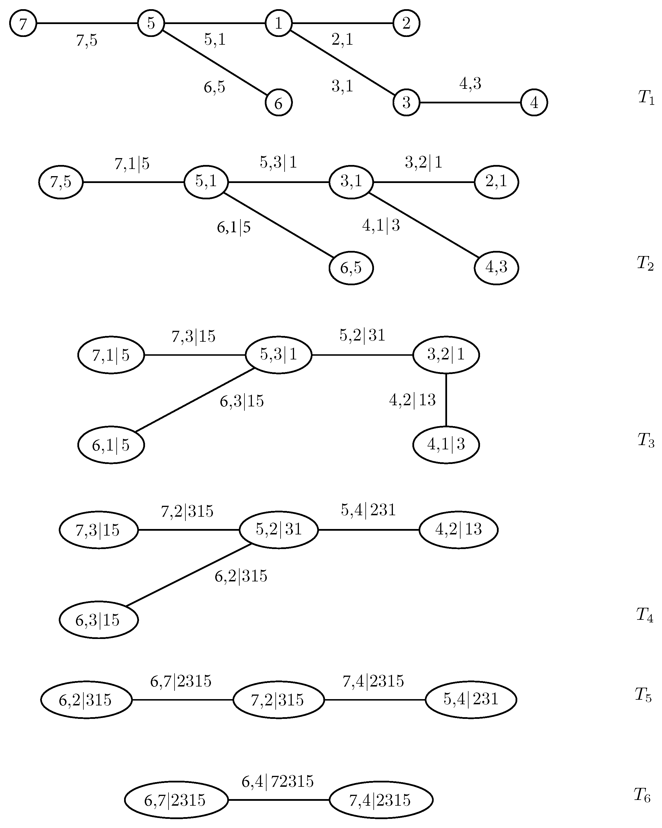
Figure 2.
A D-vine with 5 variables, 4 trees and 10 edges. Each edge may be may be associated with a pair-copula.
Figure 2.
A D-vine with 5 variables, 4 trees and 10 edges. Each edge may be may be associated with a pair-copula.
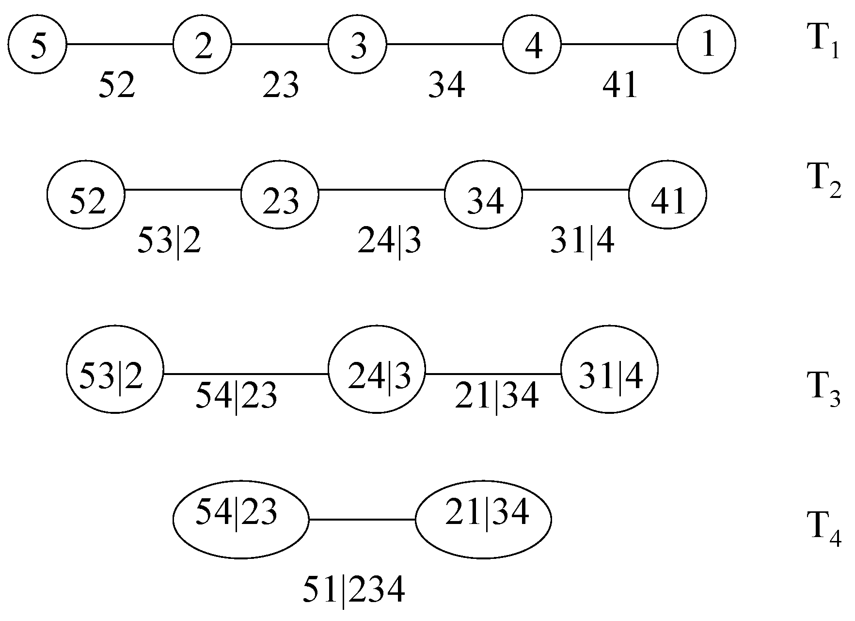
Figure 3.
A canonical vine with 5 variables, 4 trees and 10 edges. Each edge may be may be associated with a pair-copula.
Figure 3.
A canonical vine with 5 variables, 4 trees and 10 edges. Each edge may be may be associated with a pair-copula.
© 2016 by the author; licensee MDPI, Basel, Switzerland. This article is an open access article distributed under the terms and conditions of the Creative Commons Attribution (CC-BY) license ( http://creativecommons.org/licenses/by/4.0/).
Share and Cite
MDPI and ACS Style
Aas, K. Pair-Copula Constructions for Financial Applications: A Review. Econometrics 2016, 4, 43. https://doi.org/10.3390/econometrics4040043
AMA Style
Aas K. Pair-Copula Constructions for Financial Applications: A Review. Econometrics. 2016; 4(4):43. https://doi.org/10.3390/econometrics4040043
Chicago/Turabian StyleAas, Kjersti. 2016. "Pair-Copula Constructions for Financial Applications: A Review" Econometrics 4, no. 4: 43. https://doi.org/10.3390/econometrics4040043
Note that from the first issue of 2016, this journal uses article numbers instead of page numbers. See further details here.