Article

Generalized Information Matrix Tests for Detecting Model Misspecification

by
Richard M. Golden
1,*,
Steven S. Henley
2,3,6,
Halbert White
4,† and
T. Michael Kashner
3,5,6,7
1
School of Behavioral and Brain Sciences, GR4.1, 800 W. Campbell Rd., University of Texas at Dallas, Richardson, TX 75080, USA
2
Martingale Research Corporation, 101 E. Park Blvd., Suite 600, Plano, TX 75074, USA
3
Department of Medicine, Loma Linda University School of Medicine, Loma Linda, CA 92357, USA
4
Department of Economics, University of California San Diego, La Jolla, CA 92093, USA
5
Office of Academic Affiliations (10A2D), Department of Veterans Affairs, 810 Vermont Ave. NW (10A2D), Washington, DC 20420, USA
6
Center for Advanced Statistics in Education, VA Loma Linda Healthcare System, Loma Linda, CA 92357, USA
7
Department of Psychiatry, University of Texas Southwestern Medical Center at Dallas, Dallas, TX 75390, USA
*
Author to whom correspondence should be addressed.
Halbert White sadly passed away before this article was published.
Econometrics 2016, 4(4), 46; https://doi.org/10.3390/econometrics4040046
Submission received: 29 December 2015 / Revised: 13 September 2016 / Accepted: 26 October 2016 / Published: 15 November 2016
(This article belongs to the Special Issue Recent Developments of Specification Testing)

Abstract

:
Generalized Information Matrix Tests (GIMTs) have recently been used for detecting the presence of misspecification in regression models in both randomized controlled trials and observational studies. In this paper, a unified GIMT framework is developed for the purpose of identifying, classifying, and deriving novel model misspecification tests for finite-dimensional smooth probability models. These GIMTs include previously published as well as newly developed information matrix tests. To illustrate the application of the GIMT framework, we derived and assessed the performance of new GIMTs for binary logistic regression. Although all GIMTs exhibited good level and power performance for the larger sample sizes, GIMT statistics with fewer degrees of freedom and derived using log-likelihood third derivatives exhibited improved level and power performance.

1. Introduction

If a researcher’s probability model of the observed data is not correctly specified, then the interpretation of its parameter estimates may not be valid, leading to incomplete or incorrect conclusions. Thus, whether a model is correctly specified must be considered when analyzing and interpreting data (e.g., [1,2]). This issue is critically important in econometrics as well as more general scientific inquiry. For example, in health economics, estimates of the impact of clinical treatments [3,4], care systems [5], and health policy interventions on health outcomes [6] are dependent on the underlying assumption that the model to be tested is correctly specified. Further, model misspecification testing is essential for statistical analysis of randomized control trials [7,8] and observational studies [9,10]. For these reasons, this paper introduces a unified framework for identifying, classifying, and developing a wide range of specification tests.

1.1. Information Matrix Test Methods for Detection of Model Misspecification

Assume that the data x 1 , ... , x n observed in an experiment is a realization of a sequence of independent and identically distributed d-dimensional random vectors X 1 , ... , X n with a common data generating process density p x . Let M { f ( x ; θ ) : θ Θ } denote a proposed probability model that is a collection of probability densities indexed by a k-dimensional parameter vector θ . If p x M , so that p x ( x ) = f ( x ; θ ) a . e . for some θ Θ , then M is correctly specified with respect to p x .
When M is correctly specified with respect to p x , the inverse of the asymptotic covariance matrix of the maximum likelihood estimator θ ^ n arg max i = 1 n f ( X i ; θ ) is equal to both the inverse Hessian covariance matrix A 2 E { log f ( X i ; θ ) } and the inverse Outer Product Gradient (OPG) covariance matrix B E { log f ( X i ; θ ) ( log f ( X i ; θ * ) ) T } . This classic result is called the Information Matrix Equality (see [1,2], and Theorem 4 of this paper for relevant reviews).
Let u : R k R . The notation u refers to a k-dimensional column vector of functions called the gradient whose ith element is u x i , i = 1 , ... , k . The notation 2 u refers to a k-dimensional matrix-valued function which is called the Hessian of u. The element in the ith row and jth column of 2 u is 2 u x i x j , i , j = 1 , ... , k .
As described by White [1,2], the information matrix equality may be used as the basis for a test of model misspecification. White [1] proposed the Information Matrix Test (IMT) for testing the null hypothesis that the elements of the k-dimensional Hessian and k-dimensional Outer Product Gradient (OPG) inverse asymptotic covariance matrices (denoted by A and B respectively) are equal. That is, White [1] considered the null hypothesis: H o : v e c h ( A B ) = 0 k ( k + 1 ) / 2 where 0 k ( k + 1 ) / 2 denotes a k(k + 1)/2-dimensional column vector of zeros. Rejection of this null hypothesis thus implies a violation of the information matrix equality and thus the presence of model misspecification. Moreover, as noted by White [1], it may be helpful to also consider situations where the null hypothesis is “directional.” If a directional null hypothesis is rejected, this implies H o : v e c h ( A B ) = 0 k ( k + 1 ) / 2 is rejected (but the converse of this latter statement does not hold). White [1], in particular, discussed directional IMTs that have the form: H o : S v e c h ( A B ) = 0 r where the selection matrix S R r × ( k ( k + 1 ) / 2 ) consists of r rows of a k(k + 1)/2-dimensional identity matrix. In some cases directional IMTs may have more statistical power because they are designed to identify specific types of model misspecification.
For many years, the IMT approach has not been widely used outside of linear regression modeling because various instabilities (possibly associated with large degrees of freedom) of the test were observed. Chesher [11] and Lancaster [12] demonstrated how the calculation of the third derivatives of the log-likelihood function could be avoided for the full IMT, but the effectiveness of their approach was shown in some cases to exhibit unacceptable performance in logistic regression and linear regression [13,14,15,16,17,18].

1.2. Recent Developments in Information Matrix Test Theory

An advance in the theory of information matrix testing was provided by Presnell and Boos [19] (also see, [20,21,22]), who introduced an IOS (in and out of sample) directional IMT and showed that it was effective in a variety of important situations through both theoretical analyses and simulation studies. More recently, Golden et al. [23] introduced a general unified theory for model specification testing based upon a nonlinear extension of White’s [1] approach to specification testing. The new IMTs developed within the framework of Golden et al. [23] are called Generalized Information Matrix Tests (GIMT).
In particular, Golden et al. [23] discussed the problem of testing the null hypothesis that a smooth nonlinear GIMT hypothesis function s : R k × k × R k × k R r of the Hessian and OPG inverse asymptotic covariance matrices is equal to an r-dimensional vector of zeros. That is, a GIMT tests the null hypothesis H o : s ( A , B ) = 0 r . Golden et al. [23] emphasized that different choices of GIMT hypothesis function yield different types of directional and non-directional GIMT hypotheses. Although Golden et al. [23] did not provide explicit regularity conditions and a detailed analysis of their proposed general class of GIMTs, Golden et al. [23] introduced key formal definitions, provided an informal discussion of relevant theoretical results, and reported the results of a comprehensive simulation study of a realistic epidemiological analysis problem using logistic regression for six new GIMTs that exhibited appealing level and power performance. This approach for the detection of model misspecification has now been used in observational and randomized controlled trial studies [7,8,9,10].
Since the publication of Golden et al. [23], Cho and White [24] described an important class of non-directional GIMTs and showed that each of their three test statistics for model misspecification was asymptotically distributed as a squared Gaussian random variable under the null hypothesis. In addition, Cho and White [24] provided analyses of the power of their test statistics under local and global alternatives. Zhou et al. [25] proposed a non-directional GIMT statistic for the large important class of regression models where the distribution of the response variable conditioned upon the covariates is a member of the linear exponential family. Like Cho and White [24], they showed their misspecification test statistic has only a single degree of freedom and is asymptotically distributed as a squared Gaussian random variable under the null hypothesis. Huang and Prokhorov [26] also showed how the information matrix testing framework is useful for investigating goodness-of-fit using non-directional GIMT statistics for semi-parametric probability models that are specified by copulas. All of this previous work on GIMTs can be interpreted as special cases or variants of special cases of the general framework of Golden et al. [23] for finite-dimensional smooth probability models.
This paper provides a unified framework for addressing the detection of model misspecification using a variety of GIMT statistics for a large class of finite-dimensional smooth probability models. By presenting the details of the GIMT framework and explicitly presenting the relevant regularity assumptions, it establishes the foundation for supporting research into the further development of a large class of GIMTs as well as assisting in understanding the similarities and differences between different GIMTs in the existing published statistical literature.
Our paper is organized in the following manner. In Section 2, we provide the assumptions of the GIMT framework. In Section 3, we characterize the asymptotic distribution of a large family of GIMTs for a large class of finite-dimensional smooth probability models under the assumptions and definitions in Section 2. In Section 4, we investigate the performance of new GIMTs using simulation studies developed with respect to a particular logistic regression model intended to be representative of a commonly encountered problem of model misspecification detection. Conclusions are provided in Section 5.

2. GIMT Theoretical Framework: Definitions and Assumptions

In this section, we introduce the definitions and assumptions of our formal mathematical theory of Generalized Information Matrix Tests. In most practical applications, these assumptions are often satisfied for thrice continuously differentiable probability models with a fixed number of free parameters that have locally unique solutions. Throughout, it is assumed that observations are independent and identically distributed.

2.1. Data Generating Process

Let B ( R d ) be the Borel σ-field generated by the open subsets of R d .
Assumption 1.
Data Generating Process (DGP). Let X i ,   i = 1 , 2 , ... be a sequence of independent and identically distributed (i.i.d) random vectors where X i has a common probability measure P on the measurable space ( R d , B ( R d ) ) with completion ( R d , F 0 , P 0 ) .
Let the triplet ( Ω , F o , P o ) be the probability space for the Data Generating Process (DGP).
In regression modeling applications, the first element of the d-dimensional real vector xi (a realization of Xi) may be a particular value of the outcome (dependent) variable for a regression model associated with the ith data record, the second element of xi may be the number 1 for the purpose of introducing an intercept parameter, and the remaining elements of xi may be particular values for the predictor variables associated with the ith data record, i = 1, , n.
Although Assumption 1 assumes that the observed data Xi, i = 1, 2, … are i.i.d., the theory presented here is also applicable to panel data analyses. For example, consider a situation where data are collected in a longitudinal study on a group of individuals over a period of time. Assume the observations across participants are assumed to be i.i.d., but the observations for a particular participant are neither necessarily identically distributed nor independent. Let Xit denote the observation associated with the measurement of the ith participant in the study at time index t for t = 1, ,T (where T is a fixed finite number) and i = 1, , n. The theory described in this article is applicable to evaluating the degree to which a probability model can account for the observed data X i [ X i , 1 X i , T ] , i = 1, …, n.
The following assumption of absolute continuity is now introduced to permit alternative representations of P 0 in order to represent, construct, and manipulate probability densities for data generating processes involving data samples containing combinations of discrete and continuous random variables.
Assumption 2.
Absolute Continuity. Let ν j ( x j ) be a σ-finite measure on the measurable space ( R , B ( R ) ) , j = 1, , d. Let ν j = 1 d ν j ( x j ) be a σ-finite product measure on the measurable space ( R d , B ( R d ) ) . Assume P 0 is absolutely continuous with respect to ν .
By the Radon-Nikodým Theorem, Assumption 2 guarantees the joint distribution of Xi, P0, may be represented using a Radon-Nikodým density function. The Radon-Nikodým density p x d P 0 / d ν is common to the i.i.d. random variables X i , i = 1, , n on the measurable space ( R d , B ( R d ) ) .
Assumption 2 allows the theoretical results developed here to be applicable to random vectors that contain both discrete and absolutely continuous components. If a random vector is a discrete random vector or an absolutely continuous random vector, then the Radon-Nikodým density becomes a probability mass function or an absolutely continuous probability density function and the associated measure theory notation may be avoided.

2.2. Probability Model

Let s u p p   X denote the support of X.
Assumption 3.
Parametric Densities. (i) Let Θ be a compact and non-empty subset of R k , k ; (ii) Let f : R d × Θ [ 0 , ) . For each θ in Θ , f ( ; θ ) is a density with respect to v and f ( x ; ) is continuous on Θ for each x s u p p   X ; (iii) log f ( x ; ) is continuously differentiable on Θ for each x s u p p   X ; (iv) log f ( x ; ) is twice continuously differentiable on Θ for each x s u p p   X ; (v) log f ( x ; ) is thrice continuously differentiable on Θ for each x s u p p   X .
Definition. 
Probability Model. Let f be defined as in Assumption 3(i) and Assumption 3(ii). Let F : R d × Θ [ 0 , 1 ] be defined such that for each θ in Θ , F ( ; θ ) : R d [ 0 , 1 ] is the probability distribution for X specified by density f ( ; θ ) . The set M { F ( ; θ ) : R d [ 0 , 1 ] | θ Θ } is the probability model on Θ specified by f .
Definition. 
Misspecified Model. The probability model M is misspecified when P 0 M , otherwise M is correctly specified.

2.3. Hypothesis Function

Definition. 
GIMT Hypothesis Function. Let ϒ be a compact and non-empty subset of R k × k , k . A Generalized Information Matrix Test (GIMT) Hypothesis function s : ϒ × ϒ R r has the property that if A = B , then s ( A , B ) = 0 r for every symmetric positive definite matrix A ϒ and for every symmetric positive definite matrix B ϒ .
Definition. 
Nondirectional and directional GIMT Hypothesis Functions. Let ϒ be a compact and non-empty subset of R k × k , k . A nondirectional GIMT hypothesis function s : ϒ × ϒ R r has the property A = B if and only if s ( A , B ) = 0 r for all ( A , B ) ϒ × ϒ . A directional GIMT hypothesis function is a GIMT hypothesis function that is not nondirectional.
When A : R m × n R q × r , let d A d B d v e c ( A T ) d v e c ( B T ) when it exists (e.g., [27]; also see [28,29]). Let s : ϒ × ϒ R r × 2 k 2 be defined such that for all A , B ϒ : s ( A , B ) [ s ( , B ) v e c ( A ) s ( A , ) v e c ( B ) ] when it exists.
Assumption 4.
Hypothesis Function Regularity Conditions. (i) Let ϒ be a compact and non-empty subset of R k × k , k . Let s : ϒ × ϒ R r be continuous on ϒ × ϒ ; (ii) A and B are in the interior of ϒ R k × k ; (iii) s exists and is continuous on ϒ × ϒ ; (iv) s has full row rank r on ϒ × ϒ .
In practice, Assumption 4 provides a procedure for checking if the theory described here can be applied to a proposed GIMT hypothesis function.
Definition. 
Antisymmetric GIMT Hypothesis Function. Let s : ϒ × ϒ R r be a GIMT hypothesis function satisfying Assumption 4(i), Assumption 4(ii), and Assumption 4(iii). If, in addition, s ( A , B ) = s ( B , A ) for all ( A , B ) ϒ × ϒ , then s : ϒ × ϒ R r is called an antisymmetric GIMT hypothesis function.

2.4. Notation

Let g ( x ; θ ) log f ( x ; θ ) . Let g ¯ n ( θ ) ( 1 / n ) i = 1 n g ( X i ; θ ) . Let g ^ n g ¯ n ( θ ^ n ) .
Let A ¯ n ( θ ) ( 1 / n ) i = 1 n 2 log f ( X i ; θ ) . Let A ( θ ) 2 l ( θ ) .
Let B ¯ n ( θ ) ( 1 / n ) i = 1 n g ( X i ; θ ) ( g ( X i ; θ ) ) T .
Let B ( θ ) g ( x ; θ ) ( g ( x ; θ ) ) T p x ( x ) d ν x ( x ) . Let A ^ n A ¯ n ( θ ^ n ) . Let B ^ n B ¯ n ( θ ^ n ) .
Let A = A ( θ ) . Let B = B ( θ ) . Let d x , θ ( x ; θ ) [ v e c h ( 2 log f ( x ; θ ) ) v e c h ( g ( x ; θ ) ( g ( x ; θ ) ) T ) ] .
Let d ¯ n ( θ ) = ( 1 / n ) i = 1 n d x , θ ( X i ; θ ) . Let d ^ n d ¯ n ( θ ^ n ) . Let d ¯ n d ¯ n ( θ ) .
Let d ( θ ) [ v e c h ( A ( θ ) ) v e c h ( B ( θ ) ) ] . Let d d ( θ ) .
Let the notation I k denote a k-dimensional identity matrix.
Let the duplication matrix D k : R k ( k + 1 ) / 2 R k 2 be defined such that: D k v e c h ( A ) = v e c ( A ) and the inverse duplication matrix D k : R k 2 R k ( k + 1 ) / 2 be defined such that: D k v e c ( A ) = v e c h ( A ) .
Let D k I 2 D k and let D k I 2 D k .
Let d : Θ R k ( k + 1 ) where d [ d v e c h ( A ) d θ d v e c h ( B ) d θ ] = D k [ d A d θ d B d θ ] .
Let d ¯ n ( θ ) ( 1 / n ) i = 1 n d x , θ ( X i ; θ ) . Let d ^ n d ¯ n ( θ ^ n ) . Let d d ( θ ) .

2.5. Regularity Conditions

The following Assumption 5 uses a matrix version of the standard definition of dominated by an integrable function (see Appendix A).
Assumption 5.
Domination Conditions
(i)(a) log f ( x ; θ ) is dominated on Θ with respect to p x ;
(i)(b) d log f ( x ; θ ) d θ is dominated on Θ with respect to p x ;
(i)(c) g ( x ; θ ) ( g ( x ; θ ) ) T is dominated on Θ with respect to p x ;
(i)(d) d 2 log f ( x ; θ ) d θ 2 is dominated on Θ with respect to p x ;
(ii)(a) d ( d x , θ ( x ; θ ) ) d θ is dominated on Θ with respect to p x ;
(ii)(b) d x , θ ( x ; θ ) ( d x , θ ( x ; θ ) ) T is dominated on Θ with respect to p x ;
(ii)(c) g ( x ; θ ) ( d x , θ ( x ; θ ) ) T is dominated on Θ with respect to p x ;
(iii) There exists a finite positive number K such that for all x s u p p   X and for all θ Θ : | f ( x ; θ ) p x ( x ) | K .
Assumption 5 identifies specific regularity conditions that are used here to ensure that relevant expectations exist, that integral and differentiation operators can be interchanged, and that relevant laws of large numbers are applicable.
Assumption 5(i) is used to ensure that the conclusions of Theorems 2, 3, 4, 5, 6, and 7 hold. These theorems characterize the asymptotic distribution of the quasi-maximum likelihood estimator. Assumption 5(ii) is also required to ensure that the conclusions of Theorems 6 and 7 hold which characterize the asymptotic distribution of s ( A ^ n , B ^ n ) .
A sufficient but not necessary condition for both Assumption 5(i) and Assumption 5(ii) to hold is that log f is thrice continuously differentiable on the compact set Θ, measurable in its first argument (e.g., piecewise continuous), and the support of X is bounded. The assumption that the support of X is bounded is satisfied, for example, by observational data consisting of discrete random variables. Assumptions 5(i) and Assumption 5(ii) more generally are satisfied for many commonly used finite-dimensional parametric smooth probability models for observational data modeled as combinations of both discrete and absolutely continuous random variables.
Assumption 5(iii) in conjunction with Assumptions 5(i) and Assumption 5(ii) is used in Theorem 4 to ensure that: (1) when A B this corresponds to the case of model misspecification; and (2) the correctly specified probability model implies that A = B . Thus, Assumption 5(iii) is important for ensuring the proper semantic interpretation of a GIMT result (see Proposition 1 and Theorem 4). In addition, Assumption 5(iii) in conjunction with Assumption 5(i) and Assumption 5(ii) is also used to ensure that the Lancaster-Chesher approximation holds (see Theorem 8), which provides a method for constructing GIMTs without computing the third derivative of the negative log-likelihood function.
Assumption 5(iii) can be interpreted as stating that the density f ( x ; θ ) in the probability model and the data generating process density p x ( x ) cannot be too dissimilar. A sufficient but not necessary condition for satisfying Assumption 5(iii) would be that there exists two finite positive numbers K 1 and K 2 such that for all θ Θ and for all x supp   X : f ( x ; θ ) < K 1 and p x ( x ) > K 2 . Although Assumption 5(iii) could be formulated in a slightly more general manner, we use this more specialized version for expository reasons.
The negative average log-likelihood is defined as:
l ¯ n ( θ ) n 1 i = 1 n log f ( X i ; θ ) .
When it exists, the unique global minimizer of l ¯ n ( θ ) is called the quasi-maximum likelihood estimate θ ^ n rather than a maximum likelihood estimate to allow for the possibility that f may be misspecified [1].
The negative expected log-likelihood is defined as:
l ( θ ) p x ( x ) log f ( x ; θ ) d ν ( x ) .
A global minimizer of l ( θ ) is called the pseudo-true parameter value θ because of the possibility that f may be misspecified. If there exists a θ o such that f ( ; θ 0 ) = p x ν ( x ) almost everywhere, then θ o is called a true parameter value.
Assumption 6.
Uniqueness. (i) For some θ Θ , l has a unique minimum at θ ; (ii) θ is interior to Θ.
Let H 0 : s ( A , B ) = 0 r be a particular GIMT null hypothesis specified by a given GIMT hypothesis function s. Our ultimate goal is to construct a statistical test for testing the GIMT null hypothesis H 0 : s ( A , B ) = 0 r by characterizing the asymptotic behavior of the test statistic s ^ n s ( A ^ n , B ^ n ) . Note that the GIMT hypothesis function test statistic s ^ n s ( A ^ n , B ^ n ) is an estimator of s s ( A , B ) (see Theorem 6).
Let s s ( A , B ) . Let s ^ n s ( A ^ n , B ^ n ) .
Let δ ( X i ) s D k ( d x , θ ( X i ; θ ) d ( A ) 1 g ( X i ; θ ) d ) .
Given appropriate regularity conditions, it will be shown (see Theorems 6 and 7) that the asymptotic covariance matrix of n 1 / 2 ( s ^ n s ) is the GIMT asymptotic covariance matrix
Σ s δ ( x i ) ( δ ( x i ) ) T p x ( x i ) d ν ( x i ) ,
which may be estimated by
Σ ^ s n ( 1 / n ) i = 1 n δ ^ n ( X i ) ( δ ^ n ( X i ) ) T ,
where δ ^ n ( X i ) s ^ n D k ( d x , θ ( X i ; θ ^ n ) d ^ n ( A ^ n ) 1 g ( X i ; θ ^ n ) d ^ n ) .
Assumption 7.
Positive Definiteness. (i) A is positive definite; (ii) B is positive definite; and (iii) s is positive definite.
Assumption 7(i) is a sufficient but not necessary condition for the quasi-maximum likelihood estimate to be a strict local minimizer. Assumption 7(ii) is used in order to apply the Multivariate Central Limit Theorem to characterize the asymptotic distribution of the quasi-maximum likelihood estimates. Assumption 7(iii) is used in order to apply the Multivariate Central Limit Theorem to obtain the asymptotic distribution of the GIMT statistic s ^ n . Violation of Assumption 7 is analogous to the presence of multicollinearity in classical linear regression modeling.
Assumptions 6, 7(i), and 7(ii) are often checked in practice by checking if the infinity norm of g ^ n is sufficiently small and that the condition numbers of A ^ n and B ^ n are not excessively large. In addition, it is necessary to check that the condition number of an estimator of s denoted by ^ s n (see Equation (2)) is not excessively large. Note that Assumption 4(iv) is a necessary condition for s to be positive definite. If the magnitude of the asymptotic covariance matrix of the selection test statistic s ^ n s ( A ^ n , B ^ n ) , s , is not finite or s is singular, then Assumption 7(iii) fails.

3. GIMT Theoretical Framework: Theorems and Formulas

In this section, a brief review of relevant results from classical asymptotic theory is provided (Theorems 1, 2, 3, 4, 5, 8) in conjunction with our new results in Theorems 6 and 7. Proofs of all theorems and propositions are provided in the Appendix A.

3.1. Classical Results

Theorem 1.
Estimator Measurability ([30], Lemma 2). Assume that Assumptions 1, 2, 3(i), and 3(ii) hold. Let P 0 n be the joint distribution of X 1 , ... , X n . Then for each n = 1, 2, … , there exists a measurable function θ ^ n : R d n Θ and an element, Bn, of ( B ( R d ) ) n with P 0 n ( B n ) = 1 such that for all { x 1 , , x n } B n :
l ¯ n ( θ ^ n ( { x 1 , , x n } ) ) = min θ Θ l ¯ n ( θ ) .
Theorem 2.
Estimator Consistency ([31], Theorem 2.1). Assume Assumptions 1, 2, 3(i), 3(ii), 5(i)a, and 6 hold. Then as n , θ ^ n θ with probability one.
Theorem 3.
Estimator Asymptotic Distribution ([1], Theorem 3.2; also see [32]). Assume Assumptions 1, 2, 3(i), 3(ii), 3(iii), 3(iv), 5(i), 6, 7(i), and 7(ii) hold. As n → ∞, n ( θ ^ n θ ) converges in distribution to a zero-mean Gaussian random vector with non-singular covariance matrix C ( A ) 1 B ( A ) 1 .
Theorem 4.
Contrapositive Information Matrix Equality ([1], Theorem 3.3). Assume Assumptions 1, 2, 3(i), 3(ii), 3(iii), 3(iv), 5, and 6 hold. If A B , then the probability model M { F ( ; θ ) : R d [ 0 , 1 ] | θ Θ } is misspecified.
Theorem 4 is the contrapositive statement of the familiar information matrix equality that states that if a smooth regular probability model is correctly specified, then A = B . The contrapositive statement implies that a difference between A and B indicates the presence of model misspecification.
Moreover, if the information matrix equality is violated (i.e., A B ), then the asymptotic distribution of the quasi-maximum likelihood estimator is still Gaussian centered at θ but its asymptotic covariance matrix is C ( A ) 1 B ( A ) 1 . In this case, the standard formulas for estimating the asymptotic covariance matrix of the maximum likelihood estimators based upon estimating either ( A ) 1 or ( B ) 1 are not appropriate. Thus, detecting that A B is not only useful for detecting model misspecification but also detects situations where the sandwich covariance matrix estimator C ^ n ( A ^ n ) 1 B ^ n ( A ^ n ) 1 should be used to ensure an asymptotically unbiased estimate of C ( A ) 1 B ( A ) 1 is obtained. This is important in applications when one encounters predictive, yet misspecified, models. For example, a linear regression model may have small residual errors yet the residual error term is not Gaussian.
Let C ¯ n ( θ ) ( A ¯ n ) 1 B ¯ n ( θ ) ( A ¯ n ( θ ) ) 1 . Let C ^ n C ¯ n ( θ ^ n ) .
Theorem 5.
Consistent QMLE Covariance Matrix Estimators (e.g., [1]). Assume Assumptions 1, 2, 3(i), 3(ii), 3(iii), 3(iv), 5(i), 6, 7(i) and 7(ii) hold. Then, with probability one as n : B ^ n B , ( B ^ n ) 1 ( B ) 1 , A ^ n A , ( A ^ n ) 1 ( A ) 1 , C ^ n C , and ( C ^ n ) 1 ( C ) 1 .

3.2. GIMT Statistic Asymptotic Behavior

Theorem 6.
GIMT Statistic Consistency. Assume Assumptions 1, 2, 3, 4(i), 4(ii), 4(iii), 5(i), and 6 hold. Then as n , s ^ n s with probability one. If, in addition, Assumptions 5(ii) and 7(iii) hold, then with probability one ^ s n s and ( ^ s n ) 1 ( s ) 1 as n .
The asymptotic distribution of s ^ n s ( A ^ n , B ^ n ) is described in the next theorem. Strategies for estimating s are discussed at the end of this section.
Theorem 7.
Generalized Information Matrix Wald Test. Assume Assumptions 1, 2, 3, 4, 5(i), 5(ii), 6, 7 hold with respect to a GIMT hypothesis function s : ϒ × ϒ R r and probability model M . Let W ^ n n ( s ^ n ) T ( ^ s n ) 1 ( s ^ n ) . If H 0 : s = 0 r , then W ^ n d χ r 2 as n . If H 0 : s = 0 r is false, then W ^ n as n w.p.1.
Using a Wald test approach, Theorem 7 establishes that the GIMT p-value will be consistently estimated under the null hypothesis H 0 : s = 0 r thus allowing us to bound Type 1 errors by chosen significance levels. Under the alternative hypothesis H a : s 0 r , Theorem 7 ensures that the Type 2 error goes to zero as the sample size increases with probability one.
From Theorem 4 and the definition of a GIMT Hypothesis Function s : ϒ × ϒ R r , it follows that s ( A , B ) 0 r implies the presence of model misspecification. This statement follows immediately from the definition of a GIMT hypothesis function and the conclusion of Theorem 4. It is formally presented because of its semantic importance.
Proposition 1.
Interpretation of GIMT Null and Alternative Hypotheses. Suppose the Assumptions of Theorem 4 hold. Let s be a GIMT hypothesis function. (i) If M is correctly specified, then H 0 : s = 0 r ; (ii) If H 0 : s = 0 r is false, then M is misspecified.
Proposition 1 states that for either a directional or nondirectional GIMT, evidence supporting the rejection of the null hypothesis H 0 : s = 0 r is also evidence supporting the presence of model misspecification. Note, however, the assertion that H 0 : s = 0 r is true does not necessarily imply correct model specification.

3.3. GIMT Covariance Matrix Estimators

A non-directional GIMT covariance matrix estimator Σ ¨ s n is defined as an estimator with the following two properties: (i) Σ ¨ s n Σ s as n with probability one when A = B ; and (ii) Σ ¨ s n converges to a positive definite matrix as n with probability one regardless of whether the probability model is correctly specified. Property (ii) is analogous to Assumption 7(iii) and can be empirically checked by examining the condition number of the GIMT covariance matrix estimator Σ ¨ s n .
Let the Lancaster-Chesher 3rd Derivative Formula ¨ d : Θ R k ( k + 1 ) × k be defined such that:
¨ d n ( θ ) = D k [ d B ¯ n ( θ ) d θ + n 1 i = 1 n v e c ( A ( X i ; θ ) B ( X i ; θ ) ) ( g ( X i ; θ ) ) T d B ¯ n ( θ ) d θ ] ,
where
d B ¯ n ( θ ) d θ = n 1 i = 1 n [ ( A ( X i ; θ ) g ( X i ; θ ) ) + ( g ( X i ; θ ) A ( X i ; θ ) ) ] .
The formulas for the GIMT covariance matrix estimator require computation of both the second and third derivatives of the negative log-likelihood function, which are represented in Equations (1) and (2) by the formula d . Theorem 8 shows that the formula ¨ d ^ n ¨ d n ( θ ^ n ) , which uses only first and second derivatives of the negative average log-likelihood, may be used to asymptotically approximate d for the purpose of avoiding calculation of negative average log-likelihood third derivatives.
Theorem 8.
Lancaster-Chesher Estimator (see [12]). Assume Assumptions 1, 2, 3, 5(i)a, 5(i)c, 5(i)d, 5(ii)a, 5(ii)c, 5(iii), and 6 hold with respect to a GIMT hypothesis function s : ϒ × ϒ R r and probability model M . If M is correctly specified, then with probability one ¨ d n ( θ ^ n ) d as n .
Theorem 8 provides an additional mechanism for constructing alternative and possibly computationally convenient covariance matrix estimators for estimating Σ s when the null hypothesis that the model is correctly specified holds. In particular, the formula ¨ d n ( θ ^ n ) is substituted for d ^ n in Equation (2) to obtain a real symmetric matrix with non-negative eigenvalues called the Lancaster-Chesher covariance matrix estimator. If the null hypothesis that the model is correctly specified is false, then the Lancaster-Chesher covariance matrix estimator simply needs to converge to any finite positive definite matrix. This latter assumption can be empirically checked by examining the condition number of the Lancaster-Chesher covariance matrix estimator.
We now provide formulas for a variety of different types of non-directional GIMT covariance matrix estimators. First note that when the probability model is correctly specified, the contrapositive of Theorem 4 in conjunction with Theorem 5 implies that A ^ 1 = B ^ 1 = C ^ . Thus, one can use either the OPG inverse Hessian estimator B ^ 1 or the sandwich inverse Hessian estimator C ^ n as alternative estimators for the inverse Hessian estimator A ^ 1 in (2). Second, if the GIMT selection function s is anti-symmetric and A = B , then it follows that the term ( s ) D k d = 0 r so that the centering term d in (1) can be set equal to 0 r . Thus, an alternative estimator of d that can be used instead of the centering term estimator d ^ n in (2) is simply a vector of zeros. These two methods yield six different non-directional GIMT covariance matrix estimators.
Six additional GIMT covariance matrix estimators can be obtained by using the Lancaster-Chesher estimator ¨ d ^ n (defined above) as an alternative estimator for the third derivative negative average log-likelihood estimator d ^ n . The Lancaster-Chesher estimator ¨ d ^ n has the computational advantage relative to d ^ n that only the first and second derivatives of the negative log-likelihood are used. However, previous empirical studies have suggested that the use of the Lancaster-Chesher estimator ¨ d ^ n instead of the third-derivative negative average log-likelihood estimator d ^ n may degrade performance in some cases (e.g., [13,15,16,17,18]).

3.4. Adjusted GIMT Hypothesis Functions

Assumption 7(iii) requires that Σ s is a positive definite matrix. The GIMT selection function s may have the property that the r-dimensional matrix Σ s is singular with rank g where g < r so that Assumption 7(iii) fails. However, it is often possible to replace the original GIMT hypothesis function s : ϒ × ϒ R r with an alternative “adjusted” GIMT hypothesis function s : ϒ × ϒ R g that tests a similar null hypothesis yet has the properties that: (i) the resulting asymptotic covariance matrix of n 1 / 2 s n is nonsingular; and (ii) rejection of H 0 : s ( A , B ) = 0 r implies rejection of H 0 : s ( A , B ) = 0 r .
Proposition 2.
Adjusted GIMT Hypothesis Function Properties. Let Σ s be an r-dimensional GIMT asymptotic covariance matrix for GIMT hypothesis function s : ϒ × ϒ R r such that Assumption 7(iii) holds. Let the g rows of the rank g matrix T R g × r be r-dimensional orthonormal eigenvectors of Σ s ( r > g 1 ) for GIMT hypothesis function s. Define an alternative GIMT hypothesis function s T s whose respective g-dimensional GIMT asymptotic covariance matrix is Σ T = T Σ s T T . (i) If H 0 : s ( A , B ) = 0 g is false, then H 0 : s ( A , B ) = 0 r is false; (ii) The g-dimensional GIMT asymptotic covariance matrix, Σ T , for s is finite and positive definite.
The matrix T in Proposition 1 is called the adjusted GIMT hypothesis projection matrix. The proof of Proposition 2(i) follows from the observation that if | s | 2 = 0 r , then | s | 2 = 0 g . Proposition 2(ii) follows from the observation that Σ T = T Σ s T T is non-singular by the construction of T and Assumption 7(iii).

4. Simulation Studies

As discussed, some previously published information matrix tests for model misspecification have demonstrated good level and power performance (e.g., [19,23,24]). These tests may be viewed with respect to the GIMT framework presented here. The theoretical framework presented in Section 2 and Section 3 provides an important perspective in understanding the similarities and differences among existing misspecification tests within a unified framework. Further, these prior published empirical studies support the value of the GIMT framework by showing that GIMTs with good level and power performance can be constructed.
However, the GIMT framework in Section 2 and Section 3 is also valuable for developing entirely new GIMTs for a large class of probability models in a straightforward manner through the use of Theorems 6 and 7. To illustrate our approach to the construction and evaluation of such GIMTs, we show how Theorems 6 and 7 can be used to derive five new GIMTs. Although an important goal of these derivations was an interest in developing useful tests for model misspecification, a major reason for deriving five additional GIMTs was to demonstrate the flexibility and generality of the unified GIMT theory developed in Section 2 and Section 3 .
Next, simulation studies of the level and power performance of the new GIMTs are provided to examine the performance of the GIMTs for some specific empirical examples. This particular logistic regression modeling problem is intended to be representative of a commonly encountered situation where a relevant predictor in a regression model is not properly recoded and an irrelevant predictor is included. The simulation studies were not intended to be comprehensive but rather were designed to empirically demonstrate how the general GIMT theory (Section 2 and Section 3) can be used to develop a wide range of misspecification tests. For comparison purposes, the Adjusted Classical GIMT originally proposed by Golden et al. [23] was included as a sixth GIMT in the simulation studies.

4.1. Generalized Information Matrix Tests

4.1.1. Adjusted Classical GIMT (Directional) [23]

Suppose one desires to test the classical full Information Matrix Test hypothesis H 0 : A = B . Let Σ s be the r-dimensional GIMT asymptotic covariance matrix associated with this GIMT. Note that r = k ( k + 1 ) / 2 may be relatively large. Assume, however, that Σ s only has rank g where g < r. Because Σ s is not of full rank, the asymptotic theory developed here cannot be directly applied since Assumption 7(iii) is violated. However, following the discussion in Proposition 1, let T R g × r be a matrix with full row rank defined such that the g rows of T are r-dimensional orthonormal eigenvectors of Σ s ( r > g 1 ). Then, instead of testing the null hypothesis H 0 : A = B associated with the classical full non-directional Information Matrix Test [1], the null hypothesis H 0 : T v e c h ( A ) = T v e c h ( B ) is tested using the GIMT hypothesis function s defined such that: s ( A , B ) = T v e c h ( A B ) . The GIMT associated with this hypothesis function is called the Adjusted Classical GIMT (Directional). Golden et al. [23] provided further discussion of this GIMT and showed that it had good level and power properties using simulation studies of a realistic epidemiological data analysis problem.

4.1.2. Fisher Spectra GIMT (Directional)

The Fisher Spectra GIMT (Directional) is a new k-degree of freedom test specified by the GIMT hypothesis function s defined such that:
s ( A , B ) = d i a g ( ( A ) 1 B ) 1 k ,
which tests the null hypothesis H o : s ( A , B ) = 0 k . The notation 1 k denotes a k-dimensional column vector of ones. The d i a g : R k × k R k is defined such that d i a g ( ( A ) 1 B ) is a column vector of the on-diagonal elements of ( A ) 1 B . The degrees of freedom of this test are equal to the number of free parameters in the model. When the Information Matrix Equality holds, then ( A ) 1 B v will be the identity matrix and this GIMT tests the null hypothesis that the k on-diagonal elements of ( A ) 1 B are all equal to one. Note that the Fisher Spectra GIMT tests that the eigenvalues of the two matrices are the same but does not test the null hypothesis that the two matrices have the same eigenvectors. The Fisher Spectra GIMT presented here is similar to the Copula Eigenvalue Test [33]; however, the test statistic is different because the Fisher Spectra GIMT was not developed within a copula framework.

4.1.3. Robust Log GAIC GIMT (Directional)

The Robust Log GAIC GIMT (Directional) is a new 1-degree of freedom test specified by the GIMT hypothesis function s defined such that:
s ( A , B ) = log ( ( 1 k ) t r a c e ( ( A ) 1 B ) ) ,
which tests the null hypothesis H o : s ( A , B ) = 0. If the null hypothesis of this test is rejected, then not only does it indicate the presence of model misspecification, it mandates that one uses misspecification-robust estimation methods such as the sandwich estimator [1,32] and misspecification-robust model selection criteria such as the Generalized Akaike Information Criterion (GAIC) [34,35,36]. The GAIC that is defined by the formula: G A I C = 2 n l ^ n + 2 t r a c e ( ( A ) 1 B ) is an unbiased estimator of the expected value of the log-likelihood measure 2 n l ^ n (e.g., see Appendix of [35]). Note that the Log GAIC GIMT tests the same null hypothesis as the IOS IMT described by Presnell and Boos [19] (also see [20,21,22]); however, the test statistic is the logarithm of the IOS IMT statistic.

4.1.4. Robust Log GAIC Ratio GIMT (Directional)

The 1-degree of freedom Composite Log GAIC Ratio GIMT is specified by the GIMT hypothesis function s is defined such that:
s ( A , B ) = log ( t r a c e ( ( A ) 1 B ) t r a c e ( ( B ) 1 A ) ) ,
which tests the null hypothesis H o : s ( A , B ) = 0. The Robust Log GAIC Ratio GIMT (Directional) tests a null hypothesis similar to the null hypotheses associated with the group of non-directional 1 degree of freedom GIMTs discussed by Cho and Phillips [37] that compares the arithmetic mean and harmonic mean of the eigenvalues of the matrix ( A ) 1 B . It is also closely related to the IOS IMT discussed by Presnell and Boos [19] (also see [20,21,22]).

4.1.5. Composite Log GAIC GIMT (Nondirectional)

Lemma 1 of [37] shows that A = B if and only if t r a c e ( ( A ) 1 B ) = k   and   t r a c e ( ( B ) 1 A ) = k . This result provides a justification for a new type of GIMT called the 2-degree of freedom Composite Log GAIC GIMT (Non-Directional). The Composite Log GAIC GIMT specified by the GIMT hypothesis function s is defined such that:
s ( A , B ) = [ log ( ( 1 k ) t r a c e ( ( A ) 1 B ) ) log ( ( 1 k ) t r a c e ( ( B ) 1 A ) ) ] ,
which tests the null hypothesis H o : s ( A , B * ) = 0 2 . The Composite Log GAIC GIMT (Non-Directional) tests a null hypothesis similar to the null hypotheses associated with the group of non-directional 1 degree of freedom GIMTs discussed by Cho and Phillips [37] that compare the arithmetic mean and harmonic mean of the eigenvalues of the matrix ( A ) 1 B .

4.1.6. Composite GAIC GIMT (Non-Directional)

The Composite GAIC GIMT (Non-Directional) tests exactly the same null hypothesis as the Composite Log GAIC GIMT but does not include the log transformation. The Composite GAIC GIMT specified by the GIMT hypothesis function s is defined such that:
s ( A , B ) = [ ( 1 k ) t r a c e ( ( A ) 1 B ) 1 ( 1 k ) t r a c e ( ( B ) 1 A ) 1 ] ,
which tests the null hypothesis H o : s ( A , B ) = 0 2 . Cho and Phillips [37] have proposed the magnitude of the Composite Log GAIC GIMT as a 1-degree of freedom non-directional GIMT. Note that this GIMT is also closely related to the IOS test of [19].

4.2. Methods

4.2.1. Simulated Data Generating Processes

The level and power performance of the six GIMTs are tested using simulation methods described in [23]. First, five data samples, consisting of 1000, 2000, 4000, 8000, and 16,000 exemplars respectively, were created by random sampling a value x 1 from a uniform density on the interval [−1, 1] and sampling a value of x 2 from a binomial density. A response variable for each exemplar was randomly generated from the predictor x 1 using the “true” data generating process specified by the logistic regression model:
log ( p ( y = 1 ) p ( y = 0 ) ) = β 0 + β 1 x 1 + β 2 x 1 2 + β 3 x 1 3 ,
defined by the true coefficient values: β 0 = 1.98 ,   β 1 = 4.03 ,   β 2 = 1.73 ,   β 3 = 1.15 .
The response variable y is assigned to a value of one if the computed probability is greater than 0.5, and zero otherwise. Note that the four-parameter regression model in (5) is thus called the correctly specified model, and is used to re-estimate the true coefficient values using the “true” data generating process that is generated using (5).
We also modeled the same binary response variable in the simulated datasets using an “incorrectly” specified model specified by Equation (6):
log ( p ( y = 1 ) p ( y = 0 ) ) = β 0 + β 1 x 1 3 + β 2 | x 1 | + β 3 x 2 .
Notice that the parametric forms for the correctly (Equation (5)) and incorrectly (Equation (6)) specified models are the same, except that the incorrectly specified model (Equation (6)) omits x 1 and x 1 2 , and includes an “irrelevant predictor”, x 2 , and an incorrect transformation, | x 1 | .
Assume a large dataset is constructed by sampling from the data generating process specified by the model in (5). In the correctly specified case when the parameters of the model in (5) are estimated using the dataset generated by the model in (5), the resulting estimators for A ^ n and B ^ n are very similar in magnitude, indicating a lack of evidence of misspecification. On the other hand, in the misspecified case when the parameters of the model in (6) are estimated using the dataset generated by the model in (5), the resulting estimators for A ^ n and B ^ n are quite different, evidencing misspecification (see Theorem 4 of this paper).
In practice, researchers often choose the model that best fits the observed data using in-sample (training data) and out-of-sample (test data) log-likelihood based measures. Two models, however, can have equivalent fits to the observed data using either in-sample ( 2 n l ^ n ) or out-of-sample (GAIC) model fit measures, yet one of the models can be correctly specified while the other model is not. The data generating process and models used in the simulation studies described here are designed to illustrate this important situation.
The model in (5) when fitted to the dataset generated by (5) had approximately the same in-sample fit ( 2 n l ^ n = 9295.69 ) as the in-sample fit ( 2 n l ^ n = 9295.94 ) obtained when model (6) was fitted to the dataset generated by (5). Further, the Discrepancy Risk Model Selection Test [38,39,40,41,42,43] did not show a significant difference in the model fits for the models in (5) and (6) (Z = 0.003, p = 0.997).
In addition, using the GAIC [35,36,44] which estimates the out-sample (test data) model fit, the model in (5) when fitted to the dataset generated by (5) had approximately the same out-of-sample fit (GAIC = 9303.6) as the out-sample fit (GAIC = 9305.6) of model (6) to the data set generated by (5). The Discrepancy Risk Model Selection Test [38,39,40,41,42,43] showed no significant difference in GAIC model fits (Z = 0.028, p = 0.98). Thus, despite the presence of model misspecification, both the misspecified model and the correctly specified model provide observationally equivalent fits to the observed data, underscoring the importance of checking for model misspecification.

4.2.2. Estimation of Type 1 and Type 2 Error Rates

To evaluate the level and power performance of the six GIMTs, we estimate the percentage of times that each GIMT incorrectly rejected the null hypothesis in the correctly specified case (or GIMT level), and correctly rejected the null hypothesis in the misspecified case (GIMT power). Since the data were simulated from a known data generating process, the computation of these statistics is straightforward.
Throughout these simulation studies, a MLE was defined as a set of parameter values such that the sup norm of the gradient of the negative average log-likelihood evaluated at the MLE was less than 1 × 10⁻⁸. Further, we avoided fitting models to degenerate simulated data by omitting samples with condition numbers greater than 4.5 × 10¹⁴ to insure numerical stability. The condition number is defined as the maximum eigenvalue divided by the minimum eigenvalue of the inverse of the Hessian covariance matrix estimator. Each simulation was run until m = 10,000 simulated data samples of size n was reached. The sample sizes n for the simulated data represented 6.25%, 12.5%, 25%, 50%, and 100% of the original 16,000-member sample.

4.3. Results and Discussion

4.3.1. Type 1 Error Performance

Table 1 and Table 2 provide estimated Type 1 errors (i.e., estimated p-values using Theorem 7 and Equation (2)) computed using 10,000 simulated data samples for a sample size of n = 16,000. Empirical level (observed Type 1 error rates) are for pre-specified (nominal) significance levels: 0.01, 0.025, 0.05, and 0.10. The average number of times the null hypothesis was incorrectly rejected by a GIMT in a simulation run was used to estimate the Type 1 error rate. The standard error of the number of times the null hypothesis was incorrectly rejected was defined as the bootstrap sampling error. The average number of times the null hypothesis was incorrectly accepted by a GIMT in a simulation run was used to estimate the Type 2 error rate.
The p-values estimated in Table 1 are based upon the exact formula for the GIMT test statistic provided in Equation (2), which uses the third derivative of the log-likelihood function. Table 2 provides estimates of the Type 1 error rate using formulas that do not require the use of third derivatives of the log-likelihood function by using the Lancaster-Chesher third derivative approximation (see Theorem 8) for the Hessian covariance matrix estimator obtained by substituting the formula ¨ d ^ n as defined in Equations (3) and (4) for d ^ n in Equation (2).
Level performance in Table 1 and Table 2 was evaluated using the Mean Absolute Deviation (MAD), which is defined as the average absolute deviation between an estimated p-value and its theoretical expected asymptotic value. Directional GIMTs showed better performance (MAD = 0.013) than non-directional GIMTs (MAD = 0.44). In addition, the Lancaster-Chesher third derivative approximation method (Table 2) showed better performance (MAD = 0.034) than the analytic third derivative method (Table 1) (MAD = 0.055) for non-directional GIMTs. Level performance for directional GIMTs derived using the Lancaster-Chesher third derivative approximation method (MAD = 0.017) were comparable to directional GIMTs derived using the analytic third derivative method (MAD = 0.0084).
The improved Type 1 error estimation performance of the directional GIMTs may be due to the fact that the directional GIMT statistics had fewer degrees of freedom and thus reduced variance. One possible explanation for the good level performance of the Lancaster-Chesher third derivative approximation method is that this method uses assumptions that hold under the null hypothesis to derive an alternative GIMT covariance matrix estimator without calculating third derivatives. In simulation studies where the null hypothesis of correct model specification holds, key large sample assumptions of the Lancaster-Chesher third derivative approximation method are satisfied by construction. This suggests that, in some cases, for the purpose of estimating Type 1 errors, the Lancaster-Chesher method may be appropriate for large sample sizes. On the other hand, Taylor [18] has provided examples where the size properties of the Lancaster-Chesher method are poor.

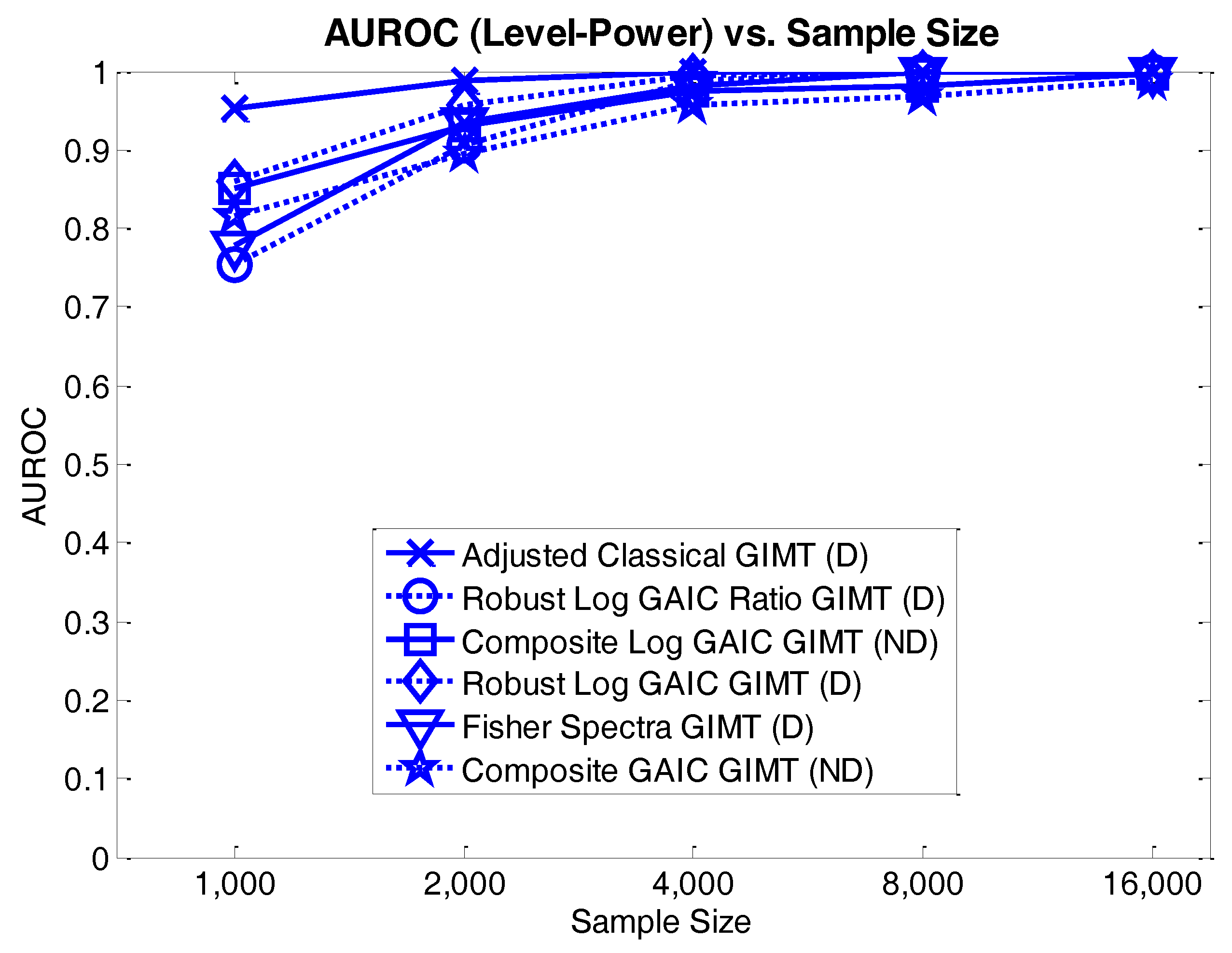
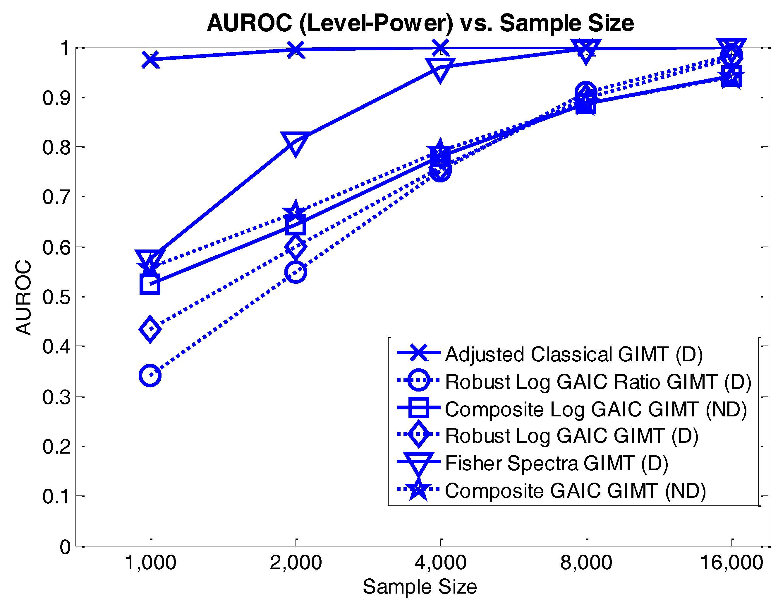
4.3.2. Level-Power Analyses

The level-power performance of the new GIMTs were investigated by examining how the estimated Type 1 and Type 2 errors varied as a function of test significance level. In particular, for a range of possible significance levels, the estimated power (i.e., percent correct rejections) and estimated Type 1 error (i.e., percent incorrect rejections) can be calculated to obtain a Receiver Operating Characteristic (ROC) curve [14,45,46,47]. The Area under the ROC (AUROC) is measure of discrimination performance. An AUROC = 1.0 indicates perfect discrimination performance and an AUROC = 0.5 indicates chance discrimination performance [45,46,47]. Although discrimination performance can vary dramatically as a function of test problem difficulty, this paradigm is useful for comparing discrimination performance of different GIMT statistics with respect to a particular test problem.
Figure 1 shows the Level-power for GIMTs using the analytic 3rd derivative for the inverse Hessian matrix estimator by sample size. With respect to the chosen test problem described in the text, these GIMTs obtain nearly perfect performance in correct rejection of the null hypothesis and correct acceptance of the null hypothesis when the sample size in this simulation study exceeds 4000 exemplars.
Figure 2 shows the Level-power for GIMTs using the Lancaster-Chesher 3rd derivative approximation. With respect to the chosen test problem these GIMTs obtain excellent performance in correct rejection of the null hypothesis and correct acceptance of the null hypothesis when the sample size in this simulation study is near 16,000 exemplars. However, while the Adjusted Classical GIMT evidences excellent performance across sample sizes in all cases, the other GIMTs show poor Level-Power performance below 15,000 exemplars with the Lancaster-Chesher 3rd derivative approximation. In addition, with the exception of the Adjusted Classical GIMT, there is not a clear difference in performance between the directional and non-directional tests. These results are consistent with the observations of previous investigators regarding the power performance of the Lancaster-Chesher method (e.g., [14,15,17,18]).

5. Conclusions

This paper formally introduces a unified framework for specification testing that is applicable to a wide range of smooth probability models including, for example, the class of generalized linear models (e.g., [48,49,50]), linear and nonlinear regression (e.g., [51,52]), structural equation models with or without latent variables (e.g., [53,54]), and hierarchical linear models (e.g., [55]). The essential idea is based upon the Contrapositive of the Information Matrix Equality (Theorem 4), which asserts that observed differences between the inverse Hessian covariance matrix estimator A ^ n and the inverse OPG covariance matrix estimator B ^ n are indicators of the presence of model misspecification.
Theorem 6 provided explicit conditions for ensuring that s ^ n converges with probability one to s ( A , B ) as n . Theorem 7 provided explicit conditions for showing that if the null hypothesis H 0 : s ( A , B ) = 0 r holds, then a Wald test statistic can be constructed that has an asymptotic chi-squared distribution with r degrees of freedom. If, however, the null hypothesis H 0 : s ( A , B ) = 0 r is false, then that same Wald test statistic asymptotically converges to infinity with probability one. Proposition 1 asserts that: (1) if the probability model is correctly specified then H 0 : s ( A , B ) = 0 r , and (2) if H 0 : s ( A , B ) = 0 r is false then the probability model is misspecified.
In the simulation studies, each of the new directional and non-directional GIMTs exhibited excellent level-power performance using the third derivative formulas for the GIMT covariance matrix estimator. However, performance in estimating the Type 1 error rate varied for different GIMTs, indicating the importance of simulation studies for characterizing the performance of new GIMTs derived within the GIMT framework. In fact, the performance of the directional GIMTs was better than the non-directional GIMTs. The simulation studies also showed that the level-power performance of the GIMTs declined with smaller sample sizes for the Lancaster-Chesher third derivative approximation formula. In addition, the appealing level-power performance of the Adjusted Classical GIMT for both the true third derivative and Lancaster-Chesher third derivative approximation suggests that additional research into the development of GIMTs with adjusted covariance matrices as described in Proposition 2 is merited. It is also important to emphasize that the alternative model used in the above power analyses was chosen such that its fit to the observed data was comparable to the fit of the “true” model that generated the data.
In summary, the simulation studies illustrate a general methodology for using the GIMT framework to derive and evaluate new model misspecification tests. We showed that it is possible for an incorrectly specified model to appear to fit the data well, while testing positive for model misspecification (i.e., reject the null hypothesis that the model is correctly specified). To reach proper statistical inferences when interpreting estimates of the parameters to a fitted model, it is critical to consider both model fit and model specification.
In conclusion, a unified GIMT framework has been presented for identifying, classifying, and developing information matrix type statistical tests for the detection of model misspecification for smooth finite-dimensional probability models. This GIMT framework provides a practical and powerful methodology for the development of both directional and non-directional GIMTs for a wide range of smooth probability models. Furthermore, unlike some existing methods for specification testing in logistic regression modeling, the degrees of freedom of the GIMT test statistic do not increase as a function of the number of distinct patterns of predictor variable values, suggesting that GIMTs will have good level and power performance [51,56,57,58]. In the real world, it is inevitable that model misspecification will manifest itself in different ways for different probability models and in different situations. Accordingly, it is desirable to have a variety of tests for assessing model misspecification as some tests may be more appropriate than others in detecting the presence of model misspecification in different situations.

Acknowledgments

This research was made possible by grants from the National Institute of General Medical Sciences (NIGMS) (R43GM114899, PI: S.S. Henley; R43GM106465, PI: S.S. Henley), the National Institute of Mental Health (NIMH) (R43MH105073, PI: S.S. Henley), the National Cancer Institute (NCI) (R44CA139607, PI: S.S. Henley), and the National Institute on Alcohol Abuse and Alcoholism (NIAAA) (R43/R44AA013768, PI: S.S. Henley; R43/R44AA013351, PI: S.S. Henley) under the Small Business Innovation Research (SBIR) program. The authors wish to gratefully acknowledge this support. This paper reflects the authors’ views and not necessarily the opinions or views of the NIGMS, NIMH, NCI, or the NIAAA.

Author Contributions

The GIMT mathematical framework was developed by Richard M. Golden and Halbert White in collaboration with Steven S. Henley and T. Michael Kashner. Richard M. Golden and Steven S. Henley developed the GIMT algorithms. The simulation studies were designed and implemented by Steven S. Henley, Richard M. Golden, and T. Michael Kashner. Halbert White did not have the opportunity to review the final version of this manuscript due to his untimely passing. Hal was a great friend and colleague who is very much missed.

Conflicts of Interest

The authors declare no conflict of interest.

Appendix A. Proofs of Theorems and Propositions

The following matrix definition of dominated by an integrable function is used in the statement and proofs of the theorems in this paper. It is provided for completeness.
Definition. 
Dominated by an Integrable Function. Let X be a random d-dimensional real vector defined on a complete probability space ( Ω , , P ) , where P has Radon-Nikodým density p with respect to a σ-finite measure ν x . Let Θ R r be a compact set, r . Let Q : R d × Θ R m × n be a function defined such that each element of Q ( x , ) is continuous on Θ for all x s u p p   X , and each element of Q ( , θ ) is measurable for all θ Θ . Suppose there exists a function K : R d R + such that each element, q i j of Q: | q i j ( x , θ ) | K ( x ) for all θ Θ and for all x s u p p   X . Also assume that the expected value of K ( X ) with respect to p is finite. Then Q is dominated by an integrable function K on Θ with respect to p .
In some cases, we will abbreviate the statement “dominated by an integrable function K on Θ with respect to p” to the statement “dominated on Θ with respect to p”.
In addition, the Dominated Convergence Theorem (e.g., [30], Theorem 2; [2], Theorem A.2.1), Slutsky’s Theorem (e.g., [59], p. 19), Mean Value Theorem (e.g., [60], p. 80), Uniform Law of Large Numbers (e.g., [2], Theorem A.2.2), and Multivariate Central Limit Theorem (e.g., [59], Theorem B, p. 28) are used throughout the following discussion.
Proof of Theorem 1.
See Lemma 2 of [30]. Q.E.D.
Proof of Theorem 2.
See Theorem 2.1 of [61]. Q.E.D.
Proof of Theorem 3.
See Theorem 3.2. of [1]. Q.E.D.
Proof of Theorem 4.
See Theorem 3.3. of [1]. Q.E.D.
Proof of Theorem 5.
See proof of Theorem 3.3 of [31]. Q.E.D.
Proof of Theorem 6.
The proof follows the approach to the proof of Theorem 4.1 in [1]. Let s ¯ n = ( A ¯ n ( θ ) , B ¯ n ( θ ) ) .
Using Assumptions 3, 4(i), 4(ii), 4(iii), and the Mean Value Theorem:
s ¯ n = s + s ¨ n D k ( d ¯ n ( θ ) d ) ,
where s ¨ n is a matrix defined such that the mth row of s is evaluated at: ( A ¨ n , B ¨ n ) ( m ) λ m ( A ¯ n ( θ ) , B ¯ n ( θ ) ) + ( 1 λ m ) ( A , B ) for some λ m ( 0 , 1 ) , m = 1, , r.
Using Assumptions 3, 4(i), 4(ii), and 4(iii), and the Mean Value Theorem:
s ^ n = s ¯ n + s n D k d n ( θ ^ n θ ) ,
where s n D k d n is a matrix constructed by evaluating the mth row of the matrix-valued function s n D k d ¯ n [ s ( A ¯ n ( θ ) , B ¯ n ( θ ) ) ] T D k d ¯ n ( θ ) at θ n γ m θ ^ n + ( 1 γ m ) θ for some γ m ( 0 , 1 ) , m = 1, , r.
Substituting (A1) into (A2) gives:
s ^ n s = s ¨ n D k ( d ¯ n ( θ ) d ) + s n D k d n ( θ ^ n θ ) .
In addition, s n = s + o p ( 1 ) because s is continuous by Assumptions 4(i), 4(ii), 4(iii) and A ˜ n A w.p.1 and B ˜ n B w.p.1 using Theorem 5. By Assumptions 3, 4, 5, and the Uniform Law of Large Numbers, s n D k d n = s D k d + o p ( 1 ) . Thus, (A3) can be rewritten as:
s ^ n s = s D k ( d ¯ n ( θ ) d ) + s D k d ( θ ^ n θ ) + o p ( 1 ) ( d ¯ n ( θ ) d ) + o p ( 1 ) ( θ ^ n θ ) .
Assumptions 1, 2, 3(i), 3(ii), 5(i)a, and 6 with Theorem 2 imply that θ ^ n θ and Assumptions 1, 2, 3(i), 3(ii), 3(iii), 3(iv), and 5(i) with the Law of Large Numbers imply that d ¯ n ( θ ) d as n with probability one. Thus, the right-hand side of (A4) approaches zero as n with probability one. The last part of Theorem 6 asserts that ^ s n s and ( ^ s n ) 1 ( s ) 1 with probability one, which follows from Assumptions 1, 2, 3, 4, 5(i), 5(ii), 6, 7 and the Uniform Law of Large Numbers. Q.E.D.
Proof of Theorem 7.
The proof follows the approach to the proof of Theorem 4.1 in [1]. Using Assumptions 3(i), 3(ii), 3(iii), 3(iv) and expand: n 1 i = 1 n g ( X i ; θ ) about θ and evaluate at θ ^ n using the Mean Value Theorem to obtain:
g ^ n = n 1 i = 1 n g ( X i ; θ * ) + A ¯ n ( θ ¨ n ) [ θ ^ n θ ]
where θ ¨ n lies on the chord connecting θ ^ n and θ . By Assumptions 1, 2, 3(i), 3(ii), 5(i)(a), and 6, and Theorem 2: θ ^ n θ with probability one as n which implies with the Uniform Law of Large Numbers: g ^ n 0 q with probability one using Assumption 5(i)(b) and A ¯ n ( θ n ) A using with probability one where A is positive definite by Assumption 7(i). By Slutsky’s Theorem, (A5), rearranging terms, and multiplying by n1/2 we then have:
n 1 / 2 ( θ ^ n θ ) = n 1 / 2 ( A ) 1 ( n 1 i = 1 n g ( X i ; θ ) ) + o p ( 1 ) .
Multiplying (13) by n 1 / 2 and substituting (A6) into Equation (A4) gives:
n 1 / 2 ( s ^ n s ) = s D k ( n 1 / 2 ( d ¯ n ( θ ) d ) d n 1 / 2 ( A ) 1 ( n 1 i = 1 n g ( X i ; θ ) ) ) s D k d o p ( 1 ) + o p ( 1 ) n 1 / 2 ( d ¯ n ( θ ) d ) + o p ( 1 ) n 1 / 2 ( θ ^ n θ ) .
Assumptions 1, 2, 3(i), 3(ii), 3(iii), 3(iv), 5(i), 6, 7(i), and 7(ii) with Theorem 3 imply that n 1 / 2 ( θ ^ n θ ) = O p ( 1 ) . Assumptions 1, 2, 3(i), 3(ii), 3(iii), 3(iv), 5(i)c, 5(i)d, and 5(ii)b in conjunction with the Dominated Convergence Theorem imply that the variance of | d x , θ ( X i , θ ) d | , V A R { | d x , θ ( X i , θ ) d | } , is finite. Thus, by the Markov Inequality, | n 1 / 2 ( d ¯ n ( θ ) d ) | = O p ( 1 ) . Thus, the last three terms on the right-hand side of (A7) converge to zero with probability one.
Pre-multiplying (A7) by the positive definite matrix ( Σ s ) 1 / 2 gives:
n 1 / 2 ( Σ s ) 1 / 2 ( s ^ n s ) = n 1 / 2 ( Σ s ) 1 / 2 s D k n 1 i = 1 n ( d x , θ ( X i ; θ ) d ( A ) 1 g ( X i ; θ ) d ) + o p ( 1 ) .
From the definition of Σ s and the assumption that Σ s is positive definite (see Assumption 7(iii)), the assumption that s has full row rank (see Assumption 4), and the Multivariate Central Limit Theorem, it follows that the first term on the right-hand side of (A8) converges in distribution to a zero mean r-dimensional multivariate Gaussian random vector Z r with an identity covariance matrix. By Slutsky’s theorem, the right-hand side of (A8) also converges to Z r in distribution and is thus bounded in probability.
If s = 0 r , then by (A8) W ^ n n ( s ^ n ) T ( s ) 1 ( s ^ n ) converges in distribution to the sum of the squares of r asymptotically normally distributed random variables (e.g., [59], p. 4) and thus has an asymptotic chi-square distribution with r degrees of freedom. If s 0 r , then W ^ n n ( s ) T ( s ) 1 ( s ) with probability one and thus W ^ n with probability one.
Finally, note that since from (A8) n 1 / 2 ( s ^ n s ) converges in distribution and thus is bounded in probability, and since from Theorem 6 s ^ s n = o p ( 1 ) we have
W ^ n = W ^ n + n ( s ^ n s ) T o p ( 1 ) ( s ^ n s ) = W ^ n + o p ( 1 ) | n 1 / 2 ( s ^ n s ) | 2 = W ^ n + o p ( 1 ) O p ( 1 ) ,
it follows from Slutsky’s Theorem that W ^ n and W ^ n have the same asymptotic distribution. Q.E.D.
Proof of Theorem 8.
The proof follows the approach of [12].
d d θ [ A ( x ; θ ) f ( x ; θ ) d ν ( x ) ] = [ d A ( x ; θ ) d θ f ( x ; θ ) + v e c ( A ( x ; θ ) ) ( d log f ( x ; θ ) d θ ) f ( x ; θ ) ]   d ν ( x )
d d θ [ B ( x ; θ ) f ( x ; θ ) d ν ( x ) ] = [ d B ( x ; θ ) d θ f ( x ; θ ) + v e c ( B ( x ; θ ) ) ( d log f ( x ; θ ) d θ ) f ( x ; θ ) ]   d ν ( x )
Differentiation under the integral operator is permitted by Assumptions 3 and 5, and the Dominated Convergence Theorem. Differentiate both sides of f ( x ; θ ) d ν ( x ) = 1 three times and use (A9) and (A10) to obtain:
d A ( x ; θ ) d θ f ( x ; θ ) d ν ( x ) = d B ( x ; θ ) d θ f ( x ; θ ) d ν ( x ) v e c ( A ( x ; θ ) B ( x ; θ ) ) ( d log f ( x ; θ ) d θ ) f ( x ; θ ) d ν ( x )
where
d B ( x ; θ ) d θ = d d θ g ( x ; θ ) g ( x ; θ ) T = ( A ( x ; θ ) g ( x ; θ ) ) + ( g ( x ; θ ) A ( x ; θ ) ) .
If the probability model is correctly specified there exists a θ such that for all x supp   X : f ( x ; θ ) = p x ( x ) ν ( x ) -almost everywhere. Let ¨ d ( θ ) [ d v e c h ( A ( x ; θ ) ) d θ f ( x ; θ ) d ν ( x ) d v e c h ( B ( x ; θ ) ) d θ f ( x ; θ ) d ν ( x ) ] .
Substituting θ into (A11) and (A12) gives the result that d = ¨ d ( θ ) when the probability model is correctly specified. The result ¨ d n ¨ d as n with probability one then follows from using the Uniform Law of Large Numbers. The result ¨ d n ( θ ^ n ) ¨ d ( θ ) follows from d n ¨ d and the result of Theorem 2, which is θ ^ n θ with probability one. Q.E.D.

References

  1. H. White. “Maximum Likelihood Estimation of Misspecified Models.” Econometrica 50 (1982): 1–25. [Google Scholar] [CrossRef]
  2. H. White. Estimation, Inference, and Specification Analysis. New York, NY, USA: Cambridge University Press, 1994. [Google Scholar]
  3. T.M. Kashner, S.S. Henley, R.M. Golden, A.J. Rush, and R.B. Jarrett. “Assessing the preventive effects of cognitive therapy following relief of depression: A methodological innovation.” J. Affect. Disord. 104 (2007): 251–261. [Google Scholar] [CrossRef] [PubMed]
  4. T.M. Kashner, R. Rosenheck, A.B. Campinell, A. Suris, R. Crandall, N.J. Garfield, P. Lapuc, K. Pyrcz, T. Soyka, and A. Wicker. “Impact of work therapy on health status among homeless, substance-dependent veterans: A randomized controlled trial.” Arch. Gen. Psychiatry 59 (2002): 938–944. [Google Scholar] [CrossRef] [PubMed]
  5. T.M. Kashner, T.J. Carmody, T. Suppes, A.J. Rush, M.L. Crismon, A.L. Miller, M. Toprac, and T. Madhukar. “Catching up on health outcomes: The Texas Medication Algorithm Project.” Health Serv. Res. 38 (2003): 311–331. [Google Scholar] [CrossRef] [PubMed]
  6. T.M. Kashner, S.S. Henley, R.M. Golden, J.M. Byrne, S.A. Keitz, G.W. Cannon, B.K. Chang, G.J. Holland, D.C. Aron, E.A. Muchmore, and et al. “Studying the Effects of ACGME Duty Hours Limits on Resident Satisfaction: Results From VA Learners’ Perceptions Survey.” Acad. Med. 85 (2010): 1130–1139. [Google Scholar] [CrossRef] [PubMed]
  7. S.S. Henley, T.M. Kashner, R.M. Golden, and A.N. Westover. “Response to letter regarding “A systematic approach to subgroup analyses in a smoking cessation trial”.” Am. J. Drug Alcohol Abuse 42 (2016): 112–113. [Google Scholar] [CrossRef] [PubMed]
  8. A.N. Westover, T.M. Kashner, T.M. Winhusen, R.M. Golden, and S.S. Henley. “A Systematic Approach to Subgroup Analyses in a Smoking Cessation Trial.” Am. J. Drug Alcohol Abuse 41 (2015): 498–507. [Google Scholar] [CrossRef] [PubMed]
  9. S.C. Brakenridge, S.S. Henley, T.M. Kashner, R.M. Golden, D. Paik, H.A. Phelan, M. Cohen, J.L. Sperry, E.E. Moore, J.P. Minei, and et al. “Comparing Clinical Predictors of Deep Venous Thrombosis vs. Pulmonary Embolus After Severe Blunt Injury: A New Paradigm for Post-Traumatic Venous Thromboembolism? ” J. Trauma Acute Care Surg. 74 (2013): 1231–1238. [Google Scholar] [CrossRef] [PubMed]
  10. S.C. Brakenridge, H.A. Phelan, S.S. Henley, R.M. Golden, T.M. Kashner, A.E. Eastman, J.L. Sperry, B.G. Harbrecht, E.E. Moore, J. Cuschieri, and et al. “Early blood product and crystalloid volume resuscitation: Risk association with multiple organ dysfunction after severe blunt traumatic injury.” J. Trauma 71 (2011): 299–305. [Google Scholar] [CrossRef] [PubMed]
  11. A. Chesher. “The information matrix test: Simplified calculation via a score test interpretation.” Econ. Lett. 13 (1983): 45–48. [Google Scholar] [CrossRef]
  12. T. Lancaster. “The Covariance Matrix of the Information Matrix Test.” Econometrica 52 (1984): 1051–1054. [Google Scholar] [CrossRef]
  13. T. Aparicio, and I. Villanua. “The asymptotically efficient version of the information matrix test in binary choice models. A study of size and power.” J. Appl. Stat. 28 (2001): 167–182. [Google Scholar] [CrossRef]
  14. R. Davidson, and J.G. MacKinnon. “Graphical Methods for Investigating the Size and Power of Hypothesis Tests.” Manch. Sch. 66 (1998): 1–26. [Google Scholar] [CrossRef]
  15. R. Davidson, and J.G. MacKinnon. “A New Form of the Information Matrix Test.” Econometrica 60 (1992): 145–157. [Google Scholar] [CrossRef]
  16. G. Dhaene, and D. Hoorelbeke. “The information matrix test with bootstrap-based covariance matrix estimation.” Econ. Lett. 82 (2004): 341–347. [Google Scholar] [CrossRef]
  17. C. Stomberg, and H. White. Bootstrapping the Information Matrix Test. Discussion Paper; San Diego, CA, USA: Department of Economics, University of California, 2000. [Google Scholar]
  18. L.W. Taylor. “The Size Bias of White’s Information Matrix Test.” Econ. Lett. 24 (1987): 63–67. [Google Scholar] [CrossRef]
  19. B. Presnell, and D.D. Boos. “The IOS Test for Model Misspecification.” J. Am. Stat. Assoc. 99 (2004): 216–227. [Google Scholar] [CrossRef]
  20. M. Capanu, and B. Presnell. “Misspecification tests for binomial and beta-binomial models.” Stat. Med. 27 (2008): 2536–2554. [Google Scholar] [CrossRef] [PubMed]
  21. M. Capanu. “Tests of Misspecification for Parametric Models.” University of Florida, 2005. Available online: http://etd.fcla.edu/UF/UFE0010943/capanu_m.pdf (accessed on 1 June 2016).
  22. S. Zhang, P.X.K. Song, D. Shi, and Q.M. Zhou. “Information ratio test for model misspecification on parametric structures in stochastic diffusion models.” Comput. Stat. Data Anal. 56 (2012): 3975–3987. [Google Scholar] [CrossRef]
  23. R.M. Golden, S.S. Henley, H. White, and T.M. Kashner. “New Directions in Information Matrix Testing: Eigenspectrum Tests.” In Causality, Prediction, and Specification Analysis: Recent Advances and Future Directions: Essays in Honor of Halbert L. White, Jr. (Festschrift Hal White Conference). Edited by X. Chen and N.R. Swanson. New York, NY, USA: Springer, 2013, pp. 145–178. [Google Scholar]
  24. J.S. Cho, and H. White. “Testing the Equality of Two Positive-Definite Matrices with Application to Information Matrix Testing.” In Essays in Honor of Peter C. B. Phillips. Edited by Y. Chang, T.B. Fomby and J.Y. Park. Bingley, UK: Emerald Group Publishing Limited, 2014, pp. 491–556. [Google Scholar]
  25. Q.M. Zhou, P.X.K. Song, and M.E. Thompson. “Information Ratio Test for Model Misspecification in Quasi-Likelihood Inference.” J. Am. Stat. Assoc. 107 (2012): 205–213. [Google Scholar] [CrossRef]
  26. W. Huang, and A. Prokhorov. “A Goodness-of-Fit Test for Copulas.” Econom. Rev. 33 (2014): 751–771. [Google Scholar] [CrossRef] [Green Version]
  27. W.H. Marlow. Mathematics for Operations Research. Mineola, NY, USA: Dover Publications, 2012. [Google Scholar]
  28. J.R. Magnus. “On the concept of matrix derivative.” J. Multivar. Anal. 101 (2010): 2200–2206. [Google Scholar] [CrossRef]
  29. J.R. Magnus, and H. Neudecker. Matrix Differential Calculus with Applications in Statistics and Econometrics. New York, NY, USA: John Wiley & Sons, 1999. [Google Scholar]
  30. R.I. Jennrich. “Asymptotic Properties of Non-linear Least Squares Estimators.” Ann. Math. Stat. 40 (1969): 633–643. [Google Scholar] [CrossRef]
  31. H. White. “Consequences and detection of misspecified nonlinear regression models.” J. Am. Stat. Assoc. 76 (1981): 419–433. [Google Scholar] [CrossRef]
  32. P. Huber. “The Behavior of Maximum Likelihood Estimates under Non-Standard Conditions.” In Proceedings Fifth Berkeley Symposium on Mathematical Statistics and Probability, Vol. 1. Berkeley, CA, USA: University of California Press, 1967, pp. 221–233. [Google Scholar]
  33. A. Prokhorov, U. Schepsmeier, and Y. Zhu. Generalized Information Matrix Tests for Copulas, Working Paper. Sydney, Australia: University of Sydney Business School, Discipline of Business Analytics, 2015. [Google Scholar]
  34. H. Bozdogan. “Model selection and Akaike’s information criterion (AIC): The general theory and its analytical extensions.” Psychometrika 52 (1987): 345–370. [Google Scholar] [CrossRef]
  35. H. Linhart, and W. Zucchini. Model Selection. New York, NY, USA: Wiley, 1986. [Google Scholar]
  36. K. Takeuchi. “Distribution of information statistics and a criterion of model fitting for adequacy of models.” Math. Sci. 153 (1976): 12–18. [Google Scholar]
  37. J. Cho, and P. Phillips. “Testing Equality of Covariance Matrices via Pythagorean Means.” 2014. Available online: http://ssrn.com/abstract=2533002 (accessed on 1 June 2016).
  38. R.M. Golden. “Statistical tests for comparing possibly misspecified and nonnested models.” J. Math. Psychol. 44 (2000): 153–170. [Google Scholar] [CrossRef] [PubMed]
  39. R.M. Golden. “Discrepancy risk model selection test theory for comparing possibly misspecified or nonnested models.” Psychometrika 68 (2003): 229–249. [Google Scholar] [CrossRef]
  40. S.S. Henley, R.M. Golden, T.M. Kashner, and H. White. Exploiting Hidden Structures in Epidemiological Data: Phase II Project. Plano, TX, USA: NIH/NIAAA, 2000. [Google Scholar]
  41. S.S. Henley, R.M. Golden, T.M. Kashner, H. White, and D. Paik. Robust Classification Methods for Categorical Regression: Phase II Project. Plano, TX, USA: National Cancer Institute, 2008. [Google Scholar]
  42. S.S. Henley, R.M. Golden, T.M. Kashner, H. White, and R.D. Katz. Model Selection Methods for Categorical Regression: Phase I Project. Plano, TX, USA: NIH/NIAAA, 2003. [Google Scholar]
  43. Q.H. Vuong. “Likelihood ratio tests for model selection and non-nested hypotheses.” Econometrica 57 (1989): 307–333. [Google Scholar] [CrossRef]
  44. H. Bozdogan. “Akaike’s Information Criterion and Recent Developments in Information Complexity.” J. Math. Psychol. 44 (2000): 62–91. [Google Scholar] [CrossRef] [PubMed]
  45. T. Fawcett. “An introduction to ROC analysis.” Pattern Recogn. Lett. 27 (2006): 861–874. [Google Scholar] [CrossRef]
  46. M.S. Pepe. The Statistical Evaluation of Medical Tests for Classification and Prediction. Oxford, UK: Oxford University Press, 2004. [Google Scholar]
  47. T.D. Wickens. Elementary Signal Detection Theory. New York, NY, USA: Oxford University Press, 2002. [Google Scholar]
  48. T. Hastie, and R. Tibshirani. Generalized Additive Models. New York, NY, USA: Chapman and Hall, 1990. [Google Scholar]
  49. P. McCullagh, and J.A. Nelder. Generalized Linear Models. London, UK: New York, NY, USA: Chapman and Hall, 1989. [Google Scholar]
  50. B. Wei. Exponential Family Nonlinear Models. New York, NY, USA: Springer, 1998. [Google Scholar]
  51. D.W. Hosmer, and S. Lemeshow. Applied Logistic Regression. New York, NY, USA: Wiley, 1989. [Google Scholar]
  52. F.E. Harrell. Regression Modeling Strategies: With Applications to Linear Models, Logistic Regression, and Survival Analysis. New York, NY, USA: Springer, 2001. [Google Scholar]
  53. G. Arminger, and M.E. Sobel. “Pseudo-maximum likelihood estimation of mean and covariance structures with missing data.” J. Am. Stat. Assoc. 85 (1990): 195–203. [Google Scholar] [CrossRef]
  54. J. Gallini. “Misspecifications that can result in path analysis structures.” Appl. Psychol. Meas. 7 (1983): 125–137. [Google Scholar] [CrossRef]
  55. S.W. Raudenbush, and A.S. Bryk. Hierarchical Linear Models: Applications and Data Analysis Methods. Thousand Oaks, CA, USA: Sage Publications, Inc., 2002. [Google Scholar]
  56. D.W. Hosmer, and S. Lemeshow. “A goodness-of-fit test for the multiple logistic regression model.” Commun. Stat. A10 (1980): 1043–1069. [Google Scholar] [CrossRef]
  57. D.W. Hosmer, S. Lemeshow, and J. Klar. “Goodness-of-Fit Testing for Multiple Logistic Regression Analysis when the Estimated Probabilities are Small.” Biom. J. 30 (1988): 1–14. [Google Scholar] [CrossRef]
  58. D.W. Hosmer, S. Taber, and S. Lemeshow. “The importance of assessing the fit of logistic regression models: A case study.” Am. J. Public Health 81 (1991): 1630–1635. [Google Scholar] [CrossRef] [PubMed]
  59. R.J. Serfling. Approximation Theorems of Mathematical Statistics. New York, NY, USA: Wiley-Interscience, 1980. [Google Scholar]
  60. H. White. Asymptotic Theory for Econometricians, Revised Edition. New York, NY, USA: Academic Press, 2001. [Google Scholar]
  61. H. White. “Using least squares to approximate unknown regression functions.” Int. Econ. Rev. 21 (1980): 149–170. [Google Scholar] [CrossRef]
Figure 1. Level-power for GIMTs using the analytic 3rd derivative formula is characterized by Area Under the Receiver Operating Characteristic curve (AUROC) as a function of sample size. With respect to the chosen test problem, these GIMTs obtain nearly perfect performance in correct rejection of the null hypothesis and correct acceptance of the null hypothesis when the sample size in this simulation study exceeds 4000 exemplars. Each data point in the above graph was generated from 10,000 bootstrap data samples.
Econometrics 04 00046 g001
Figure 2. Level-power for GIMTs using the Lancaster-Chesher 3rd derivative approximation is characterized by Area Under the Receiver Operating Characteristic curve (AUROC) as a function of sample size. With respect to the chosen test problem these GIMTs obtain excellent performance in correct rejection of the null hypothesis and correct acceptance of the null hypothesis when the sample size in this simulation study is near 16,000 exemplars. While the Adjusted Classical GIMT evidences excellent performance across sample sizes, the other GIMTs show poor Level-Power performance below 15,000 exemplars. Each data point in the above graph was generated from 10,000 bootstrap data samples.
Econometrics 04 00046 g002
Table 1. Type 1 error performance of GIMTs using the analytic third derivative formula for pre-specified (nominal) significance levels: 0.01, 0.025, 0.05, and 0.10. Level performance for the directional GIMTs was better than level performance for the non-directional GIMTs. Bootstrap simulation standard errors are shown in parentheses. Computed values are for 10,000 simulated data samples for sample size n = 16,000. df = degrees of freedom.
Generalized Information
Matrix Test (GIMT)
Test Typep = 0.01p = 0.025p = 0.05p = 0.10
Adjusted Classical (≤10 df)Directional0.01360.03080.05500.1059
(0.0012)(0.0017)(0.0023)(0.0031)
Composite GAIC (2 df)Non-Directional0.08300.10140.12250.1546
(0.0027)(0.0030)(0.0032)(0.0036)
Composite Log GAIC (2 df)Non-Directional0.05640.07420.09300.1219
(0.0023)(0.0026)(0.0029)(0.0032)
Fisher Spectra (4 df)Directional0.02050.03370.05840.1035
(0.0014)(0.0018)(0.0023)(0.0030)
Robust Log GAIC (1 df)Directional0.01850.03600.06180.1144
(0.0013)(0.0018)(0.0024)(0.0031)
Robust Log GAIC Ratio (1 df)Directional0.01580.03350.05900.1135
(0.0012)(0.0018)(0.0023)(0.0031)
Table 2. Type 1 error performance of GIMTs using the Lancaster-Chesher third derivative approximation for pre-specified (nominal) significance levels: 0.01, 0.025, 0.05, and 0.10. Like the third derivative method in Table 1, level performance for the directional GIMTs was better than level performance for the non-directional GIMTs. Further, for non-directional GIMTs, level performance of the Lancaster-Chesher third derivative approximation for the non-directional GIMTs was better than using third derivative GIMTs. Bootstrap simulation standard errors are shown in parentheses. Computed values are for 10,000 simulated data samples for sample size n = 16,000. df = degrees of freedom.
Generalized Information
Matrix Test (GIMT)
Test Typep = 0.01p = 0.025p = 0.05p = 0.10
Adjusted Classical (≤10 df)Directional0.00850.01950.04090.0916
(0.0009)(0.0014)(0.0020)(0.0029)
Composite GAIC (2 df)Non-Directional0.06620.08210.10060.1259
(0.0024)(0.0026)(0.0029)(0.0032)
Composite Log GAIC (2 df)Non-Directional0.04030.04980.06460.0884
(0.0019)(0.0021)(0.0023)(0.0027)
Fisher Spectra (4 df)Directional0.00710.01610.02640.0535
(0.0008)(0.0012)(0.0015)(0.0021)
Robust Log GAIC (1 df)Directional0.00450.01380.02360.0622
(0.0006)(0.0011)(0.0014)(0.0023)
Robust Log GAIC Ratio (1 df)Directional0.00320.00970.02850.0588
(0.0005)(0.0009)(0.0016)(0.0022)

