
The Univariate Collapsing Method for Portfolio Optimization

1
Department of Banking and Finance, University of Zurich, Zurich 8032, Switzerland
2
Swiss Finance Institute, Zurich 8006, Switzerland
Econometrics 2017, 5(2), 18; https://doi.org/10.3390/econometrics5020018
Submission received: 9 October 2016
/
Revised: 4 February 2017
/
Accepted: 17 February 2017
/
Published: 5 May 2017
Abstract
:The univariate collapsing method (UCM) for portfolio optimization is based on obtaining the predictive mean and a risk measure such as variance or expected shortfall of the univariate pseudo-return series generated from a given set of portfolio weights and multivariate set of assets under interest and, via simulation or optimization, repeating this process until the desired portfolio weight vector is obtained. The UCM is well-known conceptually, straightforward to implement, and possesses several advantages over use of multivariate models, but, among other things, has been criticized for being too slow. As such, it does not play prominently in asset allocation and receives little attention in the academic literature. This paper proposes use of fast model estimation methods combined with new heuristics for sampling, based on easily-determined characteristics of the data, to accelerate and optimize the simulation search. An extensive empirical analysis confirms the viability of the method.
1. Introduction
Determining optimal weights for a portfolio of financial assets usually first involves obtaining the multivariate predictive distribution of the returns at the future date of interest. In the classic Markowitz framework assuming independent, identically distributed (iid) Gaussian returns, “only” an estimate of the mean vector and covariance matrix are required. While this classic framework is still commonly used in industry and as a benchmark (see, e.g., Allen et al. (2016), and the references therein), it is well-known that the usual plug-in estimators of these first- and second-order moments are subject to large sampling error, and various methods of shrinkage have been successful in improving the out-of-sample performance of the asset allocation; see, e.g., Jorion (1986); Ledoit and Wolf (2004); Kan and Zhou (2007); Ledoit and Wolf (2012) for model parameter shrinkage, and DeMiguel et al. (2009a); DeMiguel et al. (2009b); Brown et al. (2013), and the references therein for portfolio weight shrinkage.
The latter two papers are concerned with the equally weighted (“”) portfolio, which can be seen as an extreme form of shrinkage such that the choice of portfolio weights does not depend on the data itself, but only the number of assets. Studies of the high performance of the equally-weighted portfolio relative to classic Markowitz allocation goes back at least to Bloomfield, et al. (1977). More recently, Fugazza et al. (2015) confirm that the “startling” performance by such a naive strategy indeed holds at the monthly level, but fails to extend to longer-term horizons, when asset return predictability is taken into account. This finding is thus very relevant for mutual- and pension-fund managers, and motivates the search for techniques to improve upon the strategy, particularly for short-term horizons such as monthly, weekly or daily.
From a theoretical perspective, DeMiguel et al. (2009b) argue that imposition of a short-sale constraint (so that all the weights are required to be non-negative, as in the portfolio) is equivalent to shrinking the expected return across assets towards their mean, while Jagannathan and Ma (2003) show that imposing a short-sale constraint on the minimum-variance portfolio is equivalent to shrinking the extreme elements of the covariance matrix, and serves as a method for decreasing estimation error in mean-variance portfolio allocation. Throughout this paper, we restrict attention to the long-only case, for these reasons, and also because most small, and many large institutional investors, notably pension funds, typically do not engage in short-selling.
Another approach maintains the iid assumption, but allows for a non-Gaussian distribution for the returns: see, e.g., McNeil et al. (2005); Adcock (2010); Adcock (2014); Adcock et al. (2015); Paolella (2015a); Gambacciani and Paolella (2017) for use of the multivariate generalized hyperbolic (MGHyp), skew-Student t, skew-normal, and discrete mixture of normals (MixN), respectively. An advantage of these models is their simplicity, with the MGHyp and MixN allowing for very fast estimation via an expectation-maximization (EM) algorithm. In fact, via use of weighted likelihood, shrinkage estimation, and short data windows, the effects of volatility clustering without requiring a GARCH-type structure can be achieved: As seen in the cases of the iid MixN of Paolella (2015a) and the iid multivariate asymmetric Laplace (as a special case of the MGHyp) of Paolella and Polak (2015c); Paolella and Polak (2015d), these can outperform use of the Engle (2002) DCC-GARCH model.
The next level of sophistication entails relaxing the iid assumption and using a multivariate GARCH-type structure (MGARCH) to capture the time-varying volatilities and, possibly, the correlations. Arguably the most popular of such constructions are the CCC-GARCH model of Bollerslev (1990); the DCC-GARCH model of Engle (2002) and Engle (2009), and various extensions, such as Billio et al. (2006) and Cappiello et al. (2006); as well as the BEKK model of Engle and Kroner (1995), see also (Caporin and McAleer 2008; Caporin and McAleer 2012); and the GARCC random coefficient model of McAleer et al. (2008), which nests BEKK. The survey articles of Bauwens et al. (2006) and Silvennoinen and Teräsvirta (2009) discuss further model constructions. Most of these models assume Gaussianity. This distributional assumption was relaxed in Aas et al. (2005) using the multivariate normal inverse Gaussian (NIG); Jondeau et al. (2007, Sec. 6.2) and Wu et al. (2015), using the multivariate skew-Student density; Santos et al. (2013) using a multivariate Student’s t; Virbickaite et al. (2016) using a Dirichlet location-scale mixture of multivariate normals; and Paolella and Polak (2015b); Paolella and Polak (2015c); Paolella and Polak (2015d) using the MGHyp, the latter in a full maximum-likelihood framework.
Many other approaches exist for the non-Gaussian, non-iid (GARCH-type) case; see e.g., Bauwens et al. (2007) and Haas et al. (2009) for a multivariate mixed normal approach; Broda and Paolella (2009), Broda et al. (2013) and the references therein for use of independent components analysis; and Paolella and Polak (2015a) and the references therein for a copula-based approach. An arguable disadvantage of some of these aforementioned models is that they effectively have the same tail thickness parameter across assets (but, when applicable, differing asymmetries, and thus are still non-elliptic), which is not in accordance with evidence from real data, such as provided in Paolella and Polak (2015a). As detailed in Paolella (2014), the univariate collapsing method (hereafter, UCM) approach indirectly allows for this feature, provided that the univariate model used for forecasting the mean, the left-tail quantiles (value at risk, or VaR), and the expected shortfall (ES) of the constructed portfolio return series, is adequately specified.
We now return to our opening remark about how portfolio optimization usually first involves obtaining the multivariate predictive distribution of the returns at the future date of interest, and then, in a second step, based on that predictive distribution, determine the optimal portfolio weight vector. The UCM method does not make use of this two-step approach, but rather uses only univariate information of (potentially thousands) of candidate portfolio distributions to determine the optimal portfolio. The idea of avoiding the usual two-step approach is not new. For example, Brandt et al. (2009) propose a straightforward and successful method that directly models the portfolio weight of each asset as a function of the asset’s characteristics, such as market capitalization, book-to-market ratio, and lagged return (momentum), as in (Fama and French 1993; Fama and French 1996). In doing so, and as emphasized by those authors, they avoid the large dimensionality issue of having to model first- and, notably, second-order moments (let alone third-order moments to capture higher-order effects and asymmetries, in which case, the dimensionality explodes). We will have more to say about this important aspect below in Section 2.1. Based on their suggestion of factors, the method of Brandt et al. (2009) is particularly well-suited to monthly (as they used) or lower-frequency re-balancing. Our goal is higher frequency re-balancing, such as daily, in which case, GARCH-type effects become highly relevant, and the aforementioned three Fama/French factors are not available at this level of granularity. Recently, Fletcher (2017) has confirmed the efficacy of the Brandt et al. (2009) approach, using the largest 350 stocks in the United Kingdom. However, he finds that (i) the performance benefits are concentrated in the earlier part of the sample period and have disappeared in recent years, and (ii) there are no performance benefits in using the method based on random subsets of those 350 largest stocks.
All time series models, including the aforementioned ones and UCM, share the problem that historical prices for the current assets of interest may not be available in the past, such as bonds with particular maturities, private equity, new public companies, merger companies, etc.; see Andersen et al. (2007, p. 515) for discussion and some resolutions to this issue. As our concern herein is a methodological development, we skirt this issue by considering only equities from major indexes (in our case, the DJIA), and also ignore any associated survivorship bias issues.
A second problem, inherent to the UCM approach is, as noted by Bauwens et al. (2006, p. 143) and Christoffersen (2009, Sec. 3), the time required for obtaining the desired portfolio weight vector, as potentially thousands of candidate vectors need to be explored and, for each, the univariate GARCH-type process needs to be estimated. As such, for risk measurement, the UCM is, given its univariate nature and the availability of highly successful methods for determining the VaR and ES in such a case (see, e.g., Kuester et al. (2006)), among the most preferable of choices, whereas for risk management, which requires portfolio optimization, multivariate models should be preferred Andersen et al. (2007, p. 541). The idea is that, once the, say, MGARCH model is estimated (this itself being potentially problematic for several types of MGARCH models, for even modest numbers of assets; see below in Section 2.1 for discussion) and the predictive distribution is available, then portfolio optimization is straightforward.
We address and resolve the second issue by building on the initial UCM framework of Paolella (2014): That paper (i) provides a detailed discussion of the benefits of UCM compared to competing methods; (ii) provides a first step towards operationalizing it by employing a method for very fast estimation of the univariate GARCH-type model not requiring evaluation of the likelihood or iterative optimization methods; and (iii) introduces the concept of the ES-span. This paper augments that work to bring the methodology closer to genuine implementation. In particular, we first study the efficacy of various sampling methods and numbers of replications, in order to better determine how small the number of required samples can be taken without impacting performance. To this end, data-driven heuristics are developed to better explore the sample space. Next, several augmentations of the method are explored to enhance performance, not entailing any appreciable increase in estimation time, and with avoidance of backtest-overfitting issues in mind.
These ideas are explored in the context of an extensive study using 15 years of daily data based on the components of the DJIA. A comparison of its performance to that of common multivariate asset allocation models demonstrates that the UCM strongly outperforms them. Thus, a univariate-based approach for risk management can be superior to multivariate models—traditionally deemed necessary because they explicitly model the (possibly time-varying) covariance structure and potentially other features such as non-Gaussianity and (asymmetric) tail dependence (see, e.g., Paolella and Polak (2015b); Härdle et al. (2015); Jondeau (2016), and the references therein).
We stress here that our goal is to develop the theory to operationalize the UCM method so as to capitalize on its features, while overcoming its primary drawbacks. As such, we do not consider herein various realistic aspects of trading, such as transaction costs, the aforementioned issues of broader asset classes, survivorship bias, and various market frictions. Also, throughout, as performance measures, we inspect cumulative returns and report Sharpe ratios, though regarding the latter, it is well-known that, as a measurement of portfolio performance, it is not optimal; see, e.g., Lo (2002), Biglova et al. (2010); and Tunaru (2015). Numerous alternatives to the Sharpe ratio exist, see, e.g., Cogneau and Hübner (2009a), Cogneau and Hübner (2009b). Of those, the ones that use downside risk measures, as opposed to the variance, might be more suited in our context, as we conduct portfolio selection with respect to ES. Future work that is more attuned to actual usage and realistic performance of the UCM framework can and should account for these and related issues in real-world trading.
The remainder of this paper is as follows. Section 2 reviews the UCM method and its advantages, and discusses fast estimation of the univariate GARCH-type model used for the pseudo-return series. Section 3 is the heart of the paper, addressing the new sampling schemes and methods for portfolio optimization, using the daily percentage returns on the components of the DJIA over a 15 year period for illustration. Section 4 shows how to enhance the allocation strategy using a feature of UCM that we deem the PROFITS measure, not shared by multivariate methods. Section 5 provides a brief comparison of model performance between the UCM and other competitors. Section 6 concludes and provides ideas for future research. An appendix collects ideas with potential for improving both the mean and volatility prediction of the pseudo-return series.
2. The Univariate Collapsing Method
2.1. Motivation
The UCM involves building a pseudo-historical time series of asset returns based on a particular set of portfolio weights (precisely defined below), fitting a flexible univariate GARCH-type process to these returns, and delivering estimates of the forecasted mean and desired risk measure, such as VaR and ES. This process is repeated numerous times to explore the portfolio-weight vector space, and that vector which most closely satisfies the desired characteristics is chosen. By using an asymmetric, heavy-tailed distribution as the innovation sequence of a flexible GARCH-type model that allows for asymmetric responses to the sign of the returns, the UCM for asset allocation, as used herein, respects all the major univariate stylized facts of asset returns, as well as a multivariate aspect that many models do not address, namely non-ellipticity, as induced, for example, by differing tail thicknesses and asymmetries across assets.
This latter feature is accomplished in an indirect way, by assuming that the conditional portfolio distribution can be adequately approximated by a noncentral Student’s t distribution (NCT). If the underlying assets were to actually follow a location-scale multivariate noncentral t distribution, then their weighted convolution is also noncentral t. This motivation is highly tempered, first by the fact that the scale terms are not constant across time, but rather exhibit strong GARCH-like behavior, and it is known that GARCH processes are not closed under summation; see, e.g., Nijman and Sentana (1996). Second, the multivariate NCT necessitates that each asset has the same tail thickness (degrees of freedom), this being precisely an assumption we wish to avoid, in light of evidence against it. Third, in addition to the fact that the underlying process generating the returns is surely not precisely a multivariate noncentral t-GARCH process, even if this were a reasonable approximation locally, it is highly debatable if the process is stationary, particularly over several years.
As such, and as also remarked by Manganelli (2004), we (i) rely on the fact that the pseudo-historical time series corresponding to a particular portfolio weight vector can be very well approximated by (in our case), an NCT-APARCH process; and (ii) use shorter windows of estimation (in our case, 250 observations, or about one year of daily trading data), to account for the non-stationarity of the underlying process.
The primary benefit of the UCM is that it avoids the ever-increasing complexity, implementation, and numerical issues associated with multivariate models, particularly those that support differing tail thicknesses of the assets and embody a multivariate GARCH-type structure. With the UCM, there is no need for constrained optimization methods and all their associated problems, such as initial values, local maxima, convergence issues, specification of tolerance parameters, and necessity that the objective function be differentiable in the portfolio weights. Moreover, while a multivariate model explicitly captures features such as the covariance matrix, this necessitates estimation of many parameters, and the curse of model mis-specification can be magnified, as well as the curse of dimensionality, in the sense that, the more parameters there are to estimate, the larger is the magnitude of estimation error. Matters can be severely exacerbated in the case of multivariate GARCH constructions for time-varying volatilities and correlations. Of course, for highly parameterized models (with time-varying volatilities or not), shrinkage estimation is a notably useful method for error reduction. However, not only is the ideal method of shrinkage not known, but even if it were, the combined effect of the two curses can be detrimental to the multivariate density forecast.
2.2. Model
Consider a set of d assets for which returns are observed over a specified period of time and frequency (e.g., daily, ignoring the weekend effect for stocks). For a particular set of non-negative portfolio weights that sum to one, i.e.,
(as determined via simulation, discussed below in Section 3), the constructed portfolio return series is computed from the d time series of past observed asset returns, , as , where , , and is the return on asset i at time t. Christoffersen (2009) refers to the generated portfolio return sequence as the pseudo-historical portfolio returns, and we will use these terms interchangeably. This method was used by Manganelli (2004), who shows how to also recover information about the multivariate structure based on sensitivity analysis of the univariate model to changes in asset weights.
A time series model is then fit to , and an h-step ahead density prediction is formed, from which any measurable quantity of interest, such as the mean, variance, VaR and ES can be computed. While the variance is the classic risk measure used for portfolio optimization, more recent developments advocate use of the ES, given that real returns data are non-elliptic, in which case, mean-variance and mean-ES portfolios will differ; see Embrechts et al. (2002) and Campbell and Kräussl (2007). Assuming the density of random variable X is continuous, the -level ES of X, which we will denote as , can be expressed as the tail conditional expectation
where the -quantile of X is denoted and is such that is the -level VaR corresponding to one unit of investment. In the non-elliptic setting, the value of can influence the allocation, though we conjecture that the effect of its choice will not be decisive in cases of real interest, with a relatively large number of assets. Throughout our development herein, we use .
Observe that use of ES requires accurate VaR prediction; see, e.g., Kuester et al. (2006) and the references therein for an overview of successful methods for VaR calculation; Broda and Paolella (2011) for details on computing ES for various distributions popular in finance; Nadarajah et al. (2013) for an overview of ES and a strong literature review on estimation methods; and Embrechts and Hofert (2014) and Davis (2016) and the references therein for an outstanding account of, and some resolutions to, measurement and elicitability of VaR and ES for internal risk measurement.
To determine the portfolio weight vector that satisfies a lower bound on the expected return and, conditional on that, minimizes the ES (which we refer to as the optimal mean-ES portfolio), various candidates are generated by some optimization or simulation algorithm and, for each, we compute (i) the constructed portfolio return series; (ii) the parameter estimates of the NCT-APARCH model (this model, the reasons for its choice, and the method of its estimation, being discussed below); (iii) the h-step ahead predictive density; and (iv) its corresponding mean and ES; in particular, the parametric ES associated with the NCT distribution forecast. Vectors that satisfy the mean constraint are kept, and the vector among them that corresponds to the smallest ES is delivered.
Observe that the ES (and all other aforementioned quantities of the predicted distribution) are model-dependent, i.e., one cannot speak of the min-ES or mean-ES portfolio, but rather the min-ES or mean-ES portfolio as implied by the particular choice of model and various parameters used, such as , the sample size, etc.. The integral in the ES formula (2) can be written as with , for . So, defining and , the weak law of large numbers confirms that
Thus, a consistent (and trivially evaluated) nonparametric estimator for the (unconditional) portfolio ES is , where is calculated based on , , and q is the empirical -quantile of . While this could be used in place of the parametric choice, we opt for the latter, given our assumption that the data generating process is not constant through time, and thus a smaller window size is desirable—rendering the nonparametric estimator relatively less accurate. This idea however, could be beneficial when is not too extreme, and when the parametric assumption is such that the parametric evaluation of the ES is numerically costly.
For predicting the distribution of the h-step return of the constructed portfolio time series, we use the asymmetric power ARCH (APARCH) model, proposed in Ding et al. (1993). This is a very flexible variant of GARCH whose properties have been well-studied; see, e.g., He and Teräsvirta (1999); Ling and McAleer (2002); Karanasos and Kim (2006); Francq and Zakoïan (2010, Ch. 10). Its benefit is that it nests, with only two additional parameters over the usual Bollerslev (1986) GARCH, at least five previously proposed GARCH extensions at that time (Ding et al. 1993, p. 98), notably the popular GJR-GARCH model of Glosten et al. (1993). However, we will restrict one of these additional parameters (the power) to be two, as shown below, because the likelihood tends to be rather flat in this parameter and its choice of a fixed value between one and two makes little difference in forecasting ability. As demonstrated in Paolella and Polak (2015c) (in the context of the GJR-GARCH model but equally applicable to the APARCH construction), use of the asymmetry parameter, determined by joint estimation with the other GARCH and non-Gaussian distributional shape parameters, does lead to improved density forecasts, though only when the actual asymmetry exceeds a nonzero threshold; and otherwise should just be taken to be zero, this being a form of shrinkage estimation.
To allow for asymmetric, heavy-tailed shocks, we couple this structure with the (singly-) noncentral Student’s t distribution (hereafter, NCT) for the innovation process, as motivated and discussed in Paolella (2014). We hereafter denote the model as NCT-APARCH. In particular, let denote an NCT random variable, with location , scale , degrees of freedom , and noncentrality coefficient , which dictates the asymmetry. (See (Paolella 2007, Sec. 10.4), for a detailed presentation of derivations and computational methods for the singly- and doubly-noncentral t.) With , the scale-one, location-shifted NCT such that its mean, if it exists, is zero, is denoted
The assumed model of the constructed portfolio return series for a T-length observed data set is then given by
for , so that the mean exists, and . The evolution of the scale parameter is dictated by the APARCH(1,1) process with fixed exponent two, i.e.,
with , , and . From (3) and (4), . If , then
where is given above. In our empirical applications, only the constraint is imposed during estimation, and in all cases, was always greater than two, and rarely less than three, justifying the choice of exponent in (5).
The predictive distribution of conditional on the fitted parameters is then a location-scale , represented as the random variable , where and the predicted volatilities are generated as the usual deterministic update of (5) based on the filtered values of , , with and . The choice of the latter values is not influential unless the process is close to the stationarity border of the APARCH process; see (Mittnik and Paolella 2000, p. 316) for calculation of the border in the APARCH case for various distributions, and (Sun and Zhou 2014, p. 290) regarding the influence of .
2.3. Model Estimation and ES Computation
Estimation of the parameters in model (4) and (5) with maximum likelihood (ML) is rather slow, owing to the density of the NCT at each point being expressed as an infinite sum or indefinite integral. Maximizing the likelihood thus involves thousands of such evaluations, and as UCM requires estimating potentially thousands of such models, this will be impractical, even on modern machines or clusters. This was addressed in Krause and Paolella (2014), in which a table lookup procedure is developed, comparing (weighted sums of the difference between) sample quantiles and pre-computed theoretical quantiles of the location-zero, unit-scale distribution (that of in (4)). In addition to this procedure being essentially instantaneous, simulations confirm that the resulting estimator actually outperforms (slightly) the MLE in terms of mean squared error (MSE) for observations, while for , the MLE and table lookup procedure result in nearly equivalent MSE-values (with the MLE slightly better, in line with standard asymptotic theory).
For estimation of location term in (4), Krause and Paolella (2014) propose a simple, convergent, iterative scheme based on trimmed means, using an optimal trimming amount based on the (conditional) degrees of freedom parameter associated with the estimated NCT-APARCH model. Simulation evidence therein shows that the method results in MSE performance on par with the MLE, but without requiring likelihood evaluation or iterative optimization procedures, and is superior to use of the sample mean (which is clearly not optimal in a heavy-tailed, non-Gaussian framework), and the sample median (which is the resulting trimmed mean for , i.e., Cauchy).
With this estimator, the APARCH parameters could be estimated by ML, such that the distribution parameters and are replaced on each iteration with their estimates from the aforementioned procedure. In particular, we can estimate the model as
where KP refers to the method of Krause and Paolella (2014) for parameters , and , L is the likelihood
and contains the APARCH parameters from (5).
For a particular (as chosen by the optimization algorithm), the KP method delivers estimates of , and . However, the likelihood of the model still needs to be computed, and this requires the evaluation of the density. This can be accomplished via the saddlepoint approximation; see (Paolella 2007, Sec. 10.4; Broda and Paolella 2007). Use of this density approximation with (6) is fast, but Krause and Paolella (2014) argue via comparisons of MLE parameter estimates based on actual and simulated data that fixing the APARCH parameters to typical values for daily financial stock return data is not only adequate, but actually outperforms their estimated counterparts in terms of VaR forecasting (and justified theoretically via shrinkage estimation). These values are given as follows.
Taken all together, the resulting estimation procedure for the NCT-APARCH model is conducted in about of a second (for both and ) on a typical modern desktop computer, and depends also slightly on the granularity of the table employed for obtaining the shape parameters. Finally, the VaR and ES of the h-step ahead location-scale predictive density are determined (essentially instantaneously, given the estimated two shape parameters) via table lookup, thus avoiding root searching the cumulative distribution function (for the VaR) and evaluation of an improper integral of a heavy tailed function (for the ES). Recall that VaR and ES preserve location-scale transformations, e.g., for any probability , with as defined in (4), it is trivial to show that, for ,
Thus, for a given time series, to estimate the model parameters and calculate the VaR and ES, no general optimization method is required, but rather about three passes of the APARCH filter, computation of sample quantiles, and then two table lookup operations; this taking about th of a second in total. Thus, for every candidate portfolio weight vector entertained by the algorithm to obtain the min-ES or mean-ES portfolio, the mean and ES are delivered extraordinarily fast. This is crucial for operationalizing use of the UCM. Now we consider how to optimize the sampling.
3. Sampling Portfolio Weights
3.1. Uniform, Corner, and Near-Equally-Weighted
The primary starting point for sampling portfolio weight vectors is to obtain values that are uniform on the simplex (1). This is achieved by taking to be
as discussed in Paolella (2014) and the references therein. However, use of
is valuable for exploring other parts of the parameter space. In particular, the non-uniformity corresponding to is such that there is a disproportionate number of values close to the equally weighted portfolio. As , (10) collapses to equal weights. This is useful, recalling the discussion in the introduction regarding the ability of the equally-weighted portfolio to outperform other allocation methods. As in (10), will approach a vector of all zeroes, except for a one at the position corresponding to the largest . Thus, large values of q can be used for exploring corner solutions. Figure 1 illustrates these sampling methods via scatterplots of versus for , using points.
The effect of using of different values of q on the ES-span for two markedly different time segments of data is illustrated in Paolella (2014). In particular, during times when the assets exhibit relatively heavy tails, it is wise to explore corner solutions, because diversification becomes less effective, whereas if assets are closer to Gaussian, then the central limit theorem suggests that their sum will be even more Gaussian, and thus exhibit a very low ES, so that exploring portfolios around the equally weighted case is beneficial. Our goals are to (i) investigate the use of different sampling schemes on the out-of-sample performance of portfolio allocation; (ii) design a heuristic to optimize the sampling, such that the least number of simulations are required to obtain the desired portfolio; and (iii) further improve upon the sampling method by considering various augmentations that result in higher performance.
3.2. Objective, and First Illustration
In general, our objective is to deliver the nonnegative portfolio vector, say , that yields the lowest (in magnitude) expected shortfall of the predictive portfolio distribution of the percentage return at time given information up to time t, conditional on its expected value being greater than some positive threshold . That is,
where is given in (1), is a pre-specified probability associated with the ES (for which we take 0.05) and
for the desired annual percentage return, here calculated assuming 250 business days per year.
Observe that, by the nature of simulated-based estimation, (11) will not be exactly obtained, but only approximated. We argue that this is not a drawback: All models, including ours, are wrong w.p.1; are anyway subject to estimation error; and the portfolio delivered will depend on the chosen data set, in particular, how much past data to use and which assets to include; and, in the case of non-ellipticity, also depends on the choice of . As such, the method should be judged not on how well (11) can be evaluated per se, but rather on the out-of-sample portfolio performance, conditional on all tuning parameters and the heuristics used to calculate (11).
As a first illustration, we use the daily (percentage log) returns on 29 stocks from the DJIA-30, from 1 June 1999 to 31 December 2014. (The DJIA-30 index consists of 30 stocks, but for the dates we use, the Visa company is excluded due to its late IPO in 2008.) For this exercise, we take ; use portfolio vector samples; based on moving windows of length ; perform daily updating throughout the entire time frame of the windows; and, as throughout, ignore transaction costs. If via sampling, a portfolio cannot be found that satisfies the mean constraint, then no trading takes place.
The left panel of Figure 2 plots the cumulative returns resulting from a one dollar initial investment using the equally weighted portfolio (“exact ”); only sampling around the equally-weighted portfolio (“near- sampling”) via use of ; and using only uniform sampling. The right panel of Figure 2 is similar, but showing the result of using corner sampling, via (10), with different values of q. Both uniform and near- sampling result in performance very similar to that of the exact portfolio, though in the years 2000 to 2003, the near- sampling lost substantially relative to the others, but after that, the cumulative returns run approximately parallel.
It is interesting to observe around 2002 to 2003, the portfolio wealth decreased, while uniform and near- sampling resulted in no trading, yet the former “caught up” with uniform sampling soon after. The annualized (pseudo-)Sharpe ratios (for which we set the risk-free rate or, in related risk measures, the minimal desired return, to zero, as in Allen et al. (2016)), computed as
for each of the three sequences of returns, yields 0.38 for the exact ; 0.53 for near- sampling; and 0.61 for uniform sampling. Thus, while the total cumulative return of the exact portfolio is about the same as that of uniform sampling and use of (11) in conjunction with the NCT-APARCH model (4), (5) and (7), the latter’s Sharpe ratio is much higher, improving from 0.38 to 0.61. This is clearly due to the lack of trading during severe market downturns, such that the sampling algorithm was not able to locate a portfolio vector that satisfied the lower bound on the desired daily return.
Use of corner solutions in the right panel show that, for mild q (4, 8, and 16), the performance is roughly similar, though for , there is significantly less diversification, and it deviates substantially from the other graphs, with a terminal wealth of about . The Sharpe ratios for the corner methods decrease monotonically in q: For and 32, thety are 0.48, 0.40, 0.34, and , respectively.
3.3. Sample Size Calibration via Markowitz
A natural suggestion to determine the optimal sample size is to conduct a backtesting exercise, similar to the one described above, with ever-increasing sample sizes s, but replacing the ES in (11) with the variance, and computing the mean and variance of the constructed portfolio return series from the usual plug-in estimators of mean and variance, under an iid assumption. The optimal sample size s is then chosen as the smallest value such that the results of the sampling method are “adequately close” to those obtained from computing the portfolio solution of the usual Markowitz setting, with no short-selling, this being a convex, easily solved, optimization problem. An obvious measure is the average (over the moving windows) Euclidean distance between the analytical-optimized and sample-based optimal portfolio.
With , observe that, for some time periods (for which we use moving windows of length ), there will be no solution to the portfolio problem, and the portfolio vector consisting of all zeros is returned; i.e., trading, is not conducted on that day. The left panel of Figure 3 shows the resulting cumulative returns (including those for the equally weighted portfolio), from which we see that, even for , the UCM with uniform sampling is not able to fully reproduce the optimized portfolio vector results. They differ substantially only during periods for which the UCM method is not able to find a portfolio that satisfies the mean constraint. The average portfolio vector discrepancies, as a function of s, are plotted in the right panel. The trajectory indicates that is not yet adequate, and that the primary issue arises during periods for which relatively few random portfolios will obtain the desired mean constraint. Based on this analysis, it is clear that brute-force sampling will not be appropriate, and more clever sampling strategies are required.
3.4. Data-Driven Sampling
Based on the previous results, our first goal is to develop a simple heuristic to help optimize how the sampling is conducted; in particular, to reduce the number of required simulated portfolio vectors for adequately approximating (11). Recall that, via the KP-method discussed above for estimating the parameters of the NCT-APARCH model, obtaining point estimates for the (conditional) degrees of freedom parameters , , is very fast, and serve as proxies for the tail indices of the innovations processes associated with the individual assets. We will use two functions of these values to help steer the choice of sampling method.
Estimated values of the are constrained such that , the upper limit of 30 being imposed because beyond it, the Student’s t distribution is adequately approximated by the Gaussian. For a particular window of data, indexed by subscript t, let
where measures the central tendency of the individual tail indices; notation means that m is truncated to lie in ; is the interquartile range and measures their dispersion; denotes the ratio for corner solutions, and denotes the ratio of uniform solutions.
The idea behind (14a) is that, if is small, i.e., the data are very heavy tailed, then is closer to one, implying that relatively more corner solutions will be entertained, whereas for large, will be small, and more solutions around the equally-weighted portfolio will be drawn. To understand (14b), observe that, if all the are close together (small IQR) and low (very heavy tails), then diversification tends to be less useful, so more corner solutions should be searched. If the are close together and very high (thin tails), then the distributions of the returns are close to Gaussian and the equally weighted portfolio will be close to the minimal ES portfolio. If the are spread out (high IQR), then there is little information to help guide the search, and more emphasis should be placed on uniform sampling.
The left panel of Figure 4 plots the individual associated with the aforementioned data set of 29 stock returns, using 30 moving windows of length 250 and incremented by 125 days, along with their median and IQR values. We see that their median values move reasonably smoothly over time, ranging from about five to eleven, while their IQR can vary and change quite substantially, though it tends to be very low most of the time. Observe that, in the beginning of the data, from 2000 to 2003, both the median and IQR are very low, so that, according to our idea, relatively more corner solutions should be searched; and from Figure 2, this is precisely where there is a noticeable increase in performance when using corner solutions, with .
Based on the above heuristic idea, we suggest taking the fractions of the total number of allowed sample portfolio weights as
where the q for searching around is taken to be , and that for corner solutions is taken to be . The right panel of Figure 4 plots the resulting , and proportions (out of ) corresponding to the DJIA data. Comparing the left and right panels, we see that, when both the median and IQR are relatively low, more corner solutions are invoked. Section 3.5.1 below will investigate the performance of the data-driven sampling scheme (14) and (15).
3.5. Methodological Assessment
The exercise displayed in Figure 2 yields a rough idea of the relative performance, but is not fully indicative for several reasons. We explore these reasons now, and, in doing so, further develop the UCM methodology.
3.5.1. Performance Variation: Use of Hair Plots
The first reason that the previous analysis is incomplete is that different runs, based on , will give different results. Plotting numerous such runs for a given sampling scheme results in what we will term a “hair plot”, indicating the uncertainty resulting from the randomly chosen portfolios. Observe that, in theory, for any , as , all the sampling schemes would result in the same performance, as they would all cover the entire space and recover (11) (albeit at different rates). However, this is precisely the point of the exercise—we wish to minimize the value of s required to adequately approximate (11).
To assess the uncertainty resulting from using , Figure 5 illustrates such hair plots for different methods of sampling, using only the last five years of data, each overlaid with the exact allocation result. As expected, in all plots, the variability increases over time, but the variation is much greater for corner sampling, while that of the data-driven sampling scheme (14) and (15), hereafter DDS, in the bottom right panel, is relatively small.
The upper left plot corresponds to uniform sampling: Noteworthy is that the majority of the sequences exceed the performance of the portfolio in terms of total cumulative wealth, thus serving as our first indication that the UCM method, in conjunction with the NCT-APARCH model, has value in this regard. Moreover, the average Sharpe ratio of the eight runs with uniform sampling is 1.10, while that for the exact portfolio is 0.94. The use of corner sampling results in lower total wealth performance, particularly for . The average Sharpe ratio for corner sampling with () is 1.09 (1.02).
For the data-driven sampling (DDS) method, the average total cumulative return, over the eight runs, is virtually the same as that of the exact portfolio; but the average Sharpe ratio is 1.05. Summarizing, for these five years of data, the attained Sharpe ratio of our proposed UCM method, based on uniform sampling and DDS, are 1.10 and 1.05, respectively; these being higher than that of the exact portfolio (0.94). While it would seem that uniform sampling is thus (slightly) superior to the data-driven method, we see that the variation over the eight runs is substantially lower for the data-driven scheme compared to uniform sampling (and certainly compared to corner sampling), indicating that more than samples are required for latter sampling methods to obtain reliable results. In particular, the data-driven method has, for a given s, a higher probability of finding the portfolio weight vector that satisfies (11), whereas, with uniform sampling, it is more “hit or miss”.
Judging if the slightly higher Sharpe ratio obtained from uniform sampling is genuine, and not from sampling error, requires formally testing if the two Sharpe values are statistically different. This is far from trivial, because assessment of the distribution of the null hypothesis of equality is not well-defined: It requires assumptions on the underlying process, and it is far from obvious what this should be. Attempts at approximations exist; see, for example, Ledoit and Wolf (2008).
3.5.2. Varying the Values of and s
The second reason that the illustration in Figure 2 is not fully informative is that it is based on the use of the arbitrarily chosen value of , whereas the use of the equally-weighted portfolio is not a data-driven model at all, and does not specify any lower bound on the expected return. While has an obvious interpretation in theory, in practice, due to model mis-specification and inability of all models to garner perfect foresight, it is perhaps best to view as a tuning parameter whose choice influences performance (and the choice of diagnostic to measure performance, here the Sharpe ratio, is itself a tuning parameter and arguably somewhat subjective). The choice of number of samples, s, is also a tuning parameter, and its effect is not trivial. To assess these effects, Figure 6 shows hair plots for five values of and three values of s, now over the entire 15-year range of the data. The Sharpe ratio of the exact portfolio is, as before, 0.38, while the average Sharpe ratios over the eight runs are indicated in the titles of the plots.
As expected, the Sharpe ratios increase with , though level off between and . However, one might have also expected that, for each given , (i) the variation in the eight runs decreases as s increases; and (ii) that, as s increases, so would the Sharpe ratio, though this is not the case. The reason for this disappointing behavior stems from what happens during the severe market downturns, and is such that these two phenomena are linked: As s increases, so does the probability of finding a portfolio that satisfies the mean constraint. While this is good in general, it occurs also during the crisis periods. If no such portfolio vector can be found, then trading ceases—as occasionally happens, according to the plots. Observe that, as expected, the effect is stronger for small , as the “hurdle” is lower. For example, with , the average Sharpe ratio (over the eight runs) drops from 0.42 to 0.31, or 26%, when moving from to , while only from 0.62 to 0.55, or 11%, for . Indeed, the variation among the eight runs is often greatest in these crisis periods, whereas during market upturns, the eight lines run nearly parallel, i.e., have little variation.
Another reason for this behavior is more insidious, and will be common to all models postulated for something as complicated as predicting financial returns: In general, if the predictive model of the portfolio distribution at time were correct, then, as s increases, so would the probability of locating portfolio vectors that satisfy (11). However, the model is wrong w.p.1, and the cost of its error is exacerbated during periods of extremely high volatility and severe market downturns.
3.6. The DDS-DONT Sampling Method
The above analysis suggests a possible augmentation of the methodology, and precisely uses a feature of UCM not explicitly inherent in models that invoke optimization methods to find the optimal mean-ES portfolio. In particular, via sampling (DDS, or uniform), we have information about the relative number of portfolios that satisfy the mean constraint. It stands to reason that, if the vast majority of randomly chosen portfolios do not satisfy it, then it might be wise to forego investing. This also makes sense from the point of view that, even if the model were “reasonably specified”, and a portfolio was found that satisfies the mean constraint, the lack of perfect foresight implies that the optimal portfolio weights are subject to sampling variation, and perturbing the optimal one slightly could result in a loss, in light of the vast majority of randomly chosen ones not satisfying the mean constraint.
To operationalize this insight, let (with C for “cutoff”) indicate the upper bound such that, if the number of samples satisfying the mean constraint is less than this value, then trading is not conducted. When used with DDS, as we do, we refer to this method as UCM():DDS+DONT() or just DDS+DONT, where DONT refers to “do not trade”. Figure 7 shows the associated hair plots (left) and the smoothed Sharpe ratios as a function of (right), for the three choices of replication number, , , and . We immediately see that, for no choice of s is the variation across the runs eliminated, but the performance is clearly better. Overlaid on the graphs for and are the results of using the aggregated samples over the eight runs, e.g., for (), they are based on all 800 (2400) samples. The graphs in left panels (labeled “Aggregate”) indicate their performance with respect to cumulative returns, based on use of ().
For , the performance is virtually the same as that shown in the comparable graphic in Figure 6, along with the Sharpe ratio being the same (to two digits); and this is corroborated by the top right panel of Figure 7, showing that the optimal value for , for all (in this case, 10) runs, occurs very close to zero (value was used for the left plot). It is noteworthy that all the runs exhibit a second, though usually lower, peak, around . Now turning to , appears nearly optimal from the graphs, and is what was used to generate the hair plot (as indicated in the title and legend). In this case, the performance exceeds that of the DDS-only method, and also exceeds that of DDS+DONT with , so that we finally obtain the desired situation: as s increases, so does performance. Indeed, for , the obtained Sharpe ratio is (slightly) higher than that for , and also, unlike for the and cases, all eight of the runs result in a terminal cumulative return exceeding that of the portfolio. In this case, the optimal value of is taken to be eight. Also observe in the Sharpe ratio plots as a function of that, for all three choices of replication number, there is a local maximum around .
For any chosen tuning parameter, such as , in order to avoid the trap of backtest-overfitting (see, e.g., Zhu et al. (2017)), it is necessary (but not sufficient) that (i) the performance is approximately quadratic in around the maximum, i.e., it is approximately monotone increasing up to an area near the maximum, and then subsequently monotone decreasing, and (ii) that it is roughly constant over a range of values around the maximum. If the latter two conditions were not true, then the selection of the optimal -value would be non-robust and unreliable. Still, it must be emphasized that, in general, the choice of the optimal tuning parameter could be dependent on (i) the value of s, the number of samples, as is necessarily the case with , and (ii) d, the number of assets. (It might also depend on the data itself, and the choice of window size w, though we conjecture—and hope—that, for daily returns on liquid stock markets, this effect will be minimal.) This dependency implies that, for values of d and s other than used here, a similar exercise would need to be conducted to find a reasonable value of . Future work could attempt to determine a (simple, polynomial) relationship yielding an optimal value of s for a given d, and also then the optimal value of , for typical stock market data (and possibly other asset classes).
To further visualize the use of this cutoff strategy, the top left panel of Figure 8 shows the number of samples out of that satisfy the mean constraint. (It is based on the first of the eight runs, but they all look essentially the same.) It varies smoothly over time, but is close to or equal to zero about 15% of the time, and these periods corresponding precisely to periods of heavy market turbulence and downturns. Remarkably, the number of samples satisfying the mean constraint is close to or equal to s about of the time, suggesting a very optimistic trading environment; we will explore this feature below in Section 4.2. Below this plot are graphs of the predicted ES for the portfolio and the optimal portfolio based on DDS. As hoped, the ES of the DDS-obtained portfolio is lower than that of the portfolio almost all the time. Observe that the former are occasionally zero because no sample was found for that time segment that satisfies the mean constraint (and are not plotted, for visibility reasons).
As the UCM method results in numerous sampled portfolios throughout the portfolio space, Figure 8 also shows the expected mean, sorted over the sampled portfolios, and a scatterplot of the predictive expected return versus the predictive ES for the sampled portfolios, for time point t corresponding to the last observation in the data set (and based on the first of the eight runs). The latter gives a sense of the efficient frontier for any particular time point, though observe that, unlike in the Markowitz and other analytic frameworks, the actual frontier cannot be computed. Instead, extensive sampling would be required to find the portfolio with the highest return for a specified interval of expected shortfall risk.
4. Enhancing Performance with PROFITS
Being reasonably satisfied with the DDS+DONT sampling method, we now wish to further make use of the UCM paradigm to enhance the quality of the allocation. In particular, observe that, while the performance of DDS+DONT was shown to be superior to DDS only, it was driven primarily by the ability to avoid trading during crisis periods (itself a worthy and useful achievement), but otherwise, the cumulative return graphs run nearly parallel to the portfolio. One might argue that this is a positive finding, illustrating that, also from a mean-ES point of view, is often the best choice during non-crisis periods, complimenting numerous other arguments in favor of , as discussed in the introduction. Nevertheless, that would also imply that the UCM, and possibly many other models that were purportedly designed to capture the variety of stylized facts of asset returns, are unnecessary for asset allocation, rendering them econometric monstrosities of little value in this context. We show that, for the UCM, this is not the case.
4.1. PROFITS-Weighted Approach
The development of heuristic (14)–(15) was based on an assessment of the tail nature of the universe of assets under consideration taken as a whole. This can be further refined by a comparison between assets, attempting to place relatively more portfolio weight on certain assets whose univariate characteristics are deemed advantageous. To this end, we propose assigning the weights proportional to a ratio of return to risk. In particular, let
, where is a tuning parameter, subsequently discussed, and med refers to the median. Fraction is an obvious analog to many ratios, such as Sharpe, with expected return divided by a risk measure, but computed not for a portfolio, but rather across different assets, for a particular single point in time. We deem this object the performance ratio of individual time forecasts, or, amusingly, the PROFITS measure. Let . Then, for a generated portfolio vector , we weight it with and normalize, taking
where ⊙ denotes the element-wise product. Thus, places more weight on “appealing” assets.
Model-based approximations to values and in (16) are quickly obtained by using the fast table lookup method for estimating the NCT-APARCH model and calculating its ES using (8), as discussed above in Section 2.3. Observe that can be negative, so that, with the no-short-selling constraint, it itself cannot be used as a vehicle for weighting a candidate portfolio weight vector, and thus the cutoff at zero in in (16). Furthermore, without short-selling, interest in the mean-ES case will be concentrated on stocks with positive (and large) -values, so that those stocks with will not enter the portfolio. (In the min-ES case, but also possibly in the mean-ES case with relatively small values of , this may not be desirable, as some of these stocks might be valuable for their ability to reduce risk via relatively lower correlation with other stocks.)
We allow in (16) to invoke shrinkage, appealing to the James-Stein framework of improving mean estimation in a multivariate framework; see, e.g., Lehmann and Casella (1998) and the references therein. The amount of shrinkage towards the target (here, the vector of values) is . Observe that, for , reduces to a fixed set of constants, so that in (17), and thus does not affect the allocation, except when , in which case, the normalized ratio in (17) cannot be computed, and we (obviously) use , i.e., trading is not conducted. Furthermore, we conjecture that this technique will be “profitable” only in reasonably favorable market periods, such that a certain number of sampled portfolios satisfy the mean constraint, whereas, if the latter exceeds the threshold indicated by (so that trading takes place) but are still rather small in number relative to s, then their resulting forecasts could be overly optimistic and too risky. To this end, let denote the fraction such that the PROFITS shrinkage is applied only if at least of the samples s satisfy the mean constraint.
We term this method UCM():DDS+DONT()+PROFIT(), or, when the other parameters are clear from the context, just PROFIT(). Arguments and are tuning parameters, whose optimal values for any particular s and d (and possibly set of data) can be obtained only by investigating their effect on portfolio performance.
The right panels of Figure 9 show the resulting smoothed Sharpe ratios as a function of both and , based on , each averaged over their respective eight runs. (A larger set of and values was initially used, and confirms that the Sharpe ratios are all substantially lower outside the illustrated range.) Observe that there is a range of values around the maximum such that near-optimal performance is achieved, so that the result is not highly sensitive to the choice and, beyond that range, the function is roughly monotone decreasing. Even more encouragingly, the obtained optimal values are the same for all s shown, namely and , and, as s increases, the quadratic shape of the mesh also increases.
The left panels of Figure 9 show the associated hair plots resulting from their use, based on the same data that generated those for in Figure 7. The terminal wealth values are all higher, and the Sharpe ratio increases from (an average over the eight runs of) 0.65 to 0.78 for ; 0.69 to 0.84 for ; and 0.71 to 0.87 for , with the highest obtained result for the largest used sampling size, 900. The optimal choices of and will possibly depend on d, though so far seem to be invariant to s, and only extensive empirical analysis could determine a mapping between them, assuming the relationship holds across data sets of stock returns. Nevertheless, we have come a long way from the comparable results in Figure 6, exhibiting far poorer Sharpe ratios and terminal wealth values, and are such that their performance decreases as s increases, against our hopes and expectations.
4.2. Increasing Amid Favorable Conditions
In light of the results indicated in the top left panel of Figure 8, one is behooved to entertain portfolios with higher return during periods when most of the random portfolios satisfy the mean constraint. Various ideas suggest themselves, such as following the DDS-DONT method but increasing until the number of such exceedances reaches a certain threshold, and then choosing among those portfolios the one with the lowest ES. While that idea was found to work, we entertain a better way.
Building on benefit conveyed by the PROFITS method (16) and (17), we proceed as follows: Let be that portfolio such that in (16) is maximized. If
- the number of random portfolios satisfying the mean constraint exceeds , and
- the ES corresponding to is less than a particular cutoff value, say ,
then choose ; otherwise choose that portfolio given by PROFIT(. We term this, omitting the DDS+DONT+PROFIT preface, the method. The justification for not choosing when its ES exceeds is that, for a portfolio with high expected return and associated high relative risk (but such that its PROFITS measure is the highest), some scepticism might be justified. Figure 10 confirms this prudence, with the right panels showing the Sharpe ratio of as a function of . They exhibits a clear peak, and, conveniently, and similar to the PROFITS parameters and , the optimal value of is 2.0, for all three values of s considered. The left panel of Figure 10 demonstrates the associated hair plots based on . For all three values of s, all the hair plots exceed the cumulative returns at virtually all points in time, and yield improved Sharpe ratios, with that for () being 0.95 (1.01).
To analyze this method in more detail, Figure 11 corresponds to one of the eight runs for , showing the results of using the method. The first three graphs show the expected return, the predicted ES, and the PROFITS measure. The latter tend to be large when—unsurprisingly—the expected mean is large, but also relatively high ES. This observation motivates the use of the cutoff which, as is clear from the right panels of Figure 10, is driving the success of the method. The bottom right panel of Figure 11 shows the realized returns of DDS+DONT+ minus those of DDS+DONT. The ratio of the number of (strictly) positive returns to (strictly) negative returns is 1.11. To gain a sense of the statistical significance of this, the 95% confidence interval of that ratio, determined by applying the nonparametric bootstrap to the nonzero differences with replications, is . The results were very similar across the eight runs.
Presumably, yet higher performance could be achieved by further increasing s, asymptotically approaching the theoretically optimal performance inherent to the method. One run (as opposed to eight, and averaging) using with (as seen from the aggregate result in the right panel, second row, of Figure 7) yielded a Sharpe ratio (SR) of 1.00. A faster approximation is obtained by concatenating the stored portfolio data sets from the runs used to generate the previous analysis based on to form a data set with an effective size of : This resulted in an SR of 0.98. A similar exercise was then conducted on the data sets, choosing three of them, for an effective s of 2700. Doing so for all cases yielded an average SR of 1.00. Based on this, it appears that is apparently a realistic sampling size for .
We do not pursue this further, as the academic point has been adequately illustrated, though for actual applications, it would be advantageous to study this behavior in detail, despite the computational burden associated with the extensive backtesting exercise and the use of eight (or more) runs. Observe however, that, once the desired s (and the other tuning parameters, as they most likely depend on d, the number of assets) are obtained, computation of future optimal portfolios is fast: For, example, with , less than two minutes are required, so that larger-scale applications to higher frequency (such as 5-minutely) data are possible.
5. Performance Comparisons across Models
The goal of this short section is to provide a final comparison, or horse-race, among some competing methods for asset allocation, augmenting the lower left panel of Figure 10. Figure 12 shows the same eight UCM runs as from that panel, along with, again, the equally weighted portfolio, as well as the i.i.d. long only Markowitz allocation and the long only Markowitz allocation based on the predictive mean and covariance matrix from the Engle (2002) Gaussian DCC-GARCH model. In addition, we add the results from a new method, namely the iid mixed normal model based on minimum covariance determinant (MCD) estimation methodology, from Gambacciani and Paolella (2017).
We see that the overall best performer is the MCD method in terms of cumulative returns, and it is noteworthy that this model does not use any type of GARCH filter, but rather an iid framework, based on short windows of estimation (to account for the time-varying scale) and use of shrinkage estimation. The UCM method, however, is unique among the methods shown in its ability to avoid trading during, and the subsequent losses associated with, crisis periods. As such, it recommends itself to consider the MCD method used in conjunction with the trade/no trade rule based on the UCM.
Finally, it is imperative to note that transaction costs were not accounted for in this comparison. Besides necessarily lowering all the returns as plotted in Figure 12 (except the equally weighted, which is not affected by use of proportional transaction cost approximations), it could change their relative ranking. For example, while the two Markowitz cases of iid and DCC-GARCH result in relatively similar performance, inspection of the actual portfolio weights over time reveals that they are much more volatile for the latter, as is typical when GARCH-type filters are used, and presumably would thus induce greater transaction costs, making the DCC approach yet less competitive.
6. Conclusions
The univariate collapsing method, UCM, has several theoretical and numerical advantages compared to many multivariate models. This paper shows that it also capable of functioning admirably in an asset allocation framework, strongly outperforming the equally-weighted portfolio, as well as avoiding trading during severe market downturns. While numerous multivariate GARCH-type models exist for predicting the joint density of future returns, parameter estimation for many of them is problematic even for a modest number of assets, and prohibitive for the case considered here, with . It is thus not clear at all how such methods actually perform in terms of portfolio performance. The UCM is fully applicable and straightforward to implement for d in the hundreds.
This goal was achieved, first by establishing a method for eliciting the predictive mean and expected shortfall for a univariate series of (in our case, pseudo-) historical return series quickly and accurately. In particular, the parameter estimation and delivery of the mean, VaR and ES of the NCT-APARCH model takes about 1/40 of a second on a typical desktop computer (using one core) and, as demonstrated in Krause and Paolella (2014), the VaR performance is outstanding, superior to all considered genuine competitors such as those discussed and developed in Kuester et al. (2006).
Second, to further operationalize the UCM, we develop a data-driven sampling (DDS) method in conjunction with a simple rule for when to not trade (DONT) and, more crucially, use of the so-called PROFITS measure to enhance the selection of the portfolio vector. Naively applying uniform (or even DDS) sampling resulted in the perverse result of worse performance as s, the number of samples, increases; whereas application of the designed algorithm herein results in the expected scenario of improved performance as s increases, along with strong performance results in terms of Sharpe ratios and cumulative returns.
An obvious extension of the model is to allow for short-selling. This could improve performance during crisis times, whereas currently, our method is at least able to avoid such periods. However, it is no longer obvious how to sample the weights, though a simple idea is to randomly assign a sign to the generated weights (and then renormalize), such that the probability of a positive (negative) sign increases with the magnitude of the expected return when it is positive (negative).
Another idea one might wish to consider is to apply heuristic optimization methods (not requiring continuity, let alone differentiability, of the objective function, such as the CMAES algorithm of Hansen and Ostermeier (2001), as used in Appendix B below) in place of DDS sampling to determine the optimal portfolio. Starting values could be quickly and easily obtained based on DDS sampling for a relatively small value of s. However, such a methodology is hampered by the fact that such algorithms do not easily embody constraints, such as the sum of the portfolio weights and the ES constraint via parameter , and so penalized optimization would be required. Observe that, in genuine applications, there can be many constraints (industry- and country-specific, etc.) associated with strategic asset allocation. Thus, a first step in this direction would entail modifying the desired heuristic algorithm to embody (at least linear) constraints. Furthermore, as d increases, such algorithms (and traditional, Hessian-based ones) tend to be notoriously slow, as the usual problems of high convergence times and/or convergence to local inferior maxima arise. Of course, also for the UCM, as d increases, s will necessarily need to be larger and thus take longer, but the aforementioned problems do not arise, including the issue with constraints, as these can be trivially handled by rejecting invalid samples.
Finally, it would be useful to understand some aspects of the asymptotic behavior of the method as the sample size, T increases, and possibly in conjunction with d, the number of assets, presumably in such as way that . This would require making some assumptions on the true data generating process (DGP) including strict stationarity and ergodicity, and at least moment conditions, the validity of all of which are, as usual, difficult to verify with actual data. Such an analysis is beyond the scope of this paper (and probably that of the author). Another—less satisfying, but easier—approach is to assume a very general, flexible DGP that can be easily simulated from, with parameters loosely calibrated to real data, and assess via simulation the efficacy of the UCM methodology proposed herein, possibly being able to determine more precisely the optimal tuning parameters as a function of some aspect of the assumed DGP. Such a candidate could be a flexible, possibly time-varying copula construction with margins exhibiting heterogeneous tail behavior; see, e.g., Paolella and Polak (2015a); Härdle et al. (2015), and the references therein.
Acknowledgments
Financial Support by the Swiss National Science Foundation (SNSF) through project #150277 is gratefully acknowledged. The author thanks two anonymous referees for excellent comments and ideas that have led to an improved final manuscript; and Jochen Krause for assisting with some of the calculations in Appendix B.
Conflicts of Interest
The author declares no conflict of interest.
Appendix A. Mean Signal Improvement
We attempt to improve upon the forecasted mean, in light of its importance for asset allocation; see Chopra and Ziemba (1993). An idea without noticeable computational overhead is to use the iterative trimmed mean augmented with a weighting structure such that more recent observations in time receive relatively more weight. The idea is that the model, with its fixed location term, is misspecified, and the use of weighted estimation is a simple, fast way of approximating the (otherwise unknown) time-varying nature of the location of the asset returns. See Mittnik and Paolella (2000); Paolella and Steude (2008), and the references therein for further details and applications of this concept in the context of financial asset return density and risk prediction. By design, this procedure can also capitalize on momentum, though based on only one year (250 trading days) of data, it is not a-priori clear if it will result in higher risk adjusted returns.
The weighted trimmed mean methodology we entertain is as follows. Let
where tuning parameter , , can be determined based on the quality of out-of-sample portfolio performance, computed over a grid of values of . We apply trimming to as in Krause and Paolella (2014), and let be the resulting number of remaining observations, . Let , of length , be the index vector such that denotes the remaining pseudo returns after trimming. Finally, let
where denotes the arithmetic mean of vector . Observe that corresponds to the unweighted case, as in Krause and Paolella (2014).
To assess the change in predictive performance with respect to , we use the same DJIA index data as above, from 1999 to 2014, based on moving windows of length (and incremented by one day). The predictor of is, recalling (4), taken to be for a given value of . This is computed for all 3,673 windows, a grid of -values, and for each of the 29 return series. We compare the forecasts to the actual return at time , and compute , .
For all stocks, the resulting MSE as a function of is smooth, and either monotone or quadratic shaped, but unfortunately in only three cases is it such that the MSE assumes its lowest value for a value of . In all cases, the changes in MSE across were insignificant compared to the magnitude of the MSE. Thus, this procedure is not tenable.
Appendix B. Model Diagnostics and Alternative APARCH Specifications
Recall that the APARCH parameters of the NCT-APARCH model used to model and forecast the pseudo-historial time series are fixed at values given in (7). These are compromise values such that, besides the ensuing savings in estimation time, the resulting VaR performance in aggregate, computed over numerous moving windows, actually outperforms the use of the MLE for jointly estimating the distribution and GARCH parameters of the NCT-APARCH model; see Krause and Paolella (2014). The two alternative methods of (i) literally fixing the APARCH parameters, versus (ii) unrestricted (except for stationarity and positive scale constraints) ML-estimation can be seen as the two extremes of various continuums of estimation, such as shrinkage. It is highly likely that the best performing method lies between these two extremes, though instead of shrinkage estimation, we consider a variant such that one of two fixed sets of APARCH parameters is chosen, based on a data-driven diagnostic. The reason for this is, as with the single fixed set of parameters, speed: Besides the mechanism to decide between the two sets of values, no likelihood computations, GARCH filters, or iterative estimation methods need to be invoked.
We detail the method of obtaining an alternative set of APARCH coefficients, and the mechanism for deciding among the original, and the alternative. The latter boils down to a decision based on p-values of two tests of normality, and induces a tuning parameter, , such that performance of the method can be visualized as a function of it.
While asset returns (real or constructed) obviously do not precisely follow an NCT-APARCH(1,1) process, the favorable performance of the UCM model using it provides strong evidence that it serves as an accurate approximation to the true data generating process. Indeed, it is, within the GARCH class of models, rather flexible, allowing for heavy tails of the innovation term, and asymmetry in both the innovation term and the volatility. Conditional upon it, it is of interest to determine the adequacy of the NCT and/or APARCH estimated parameters.
Consider the following approach for the former: Starting with iid NCT realizations, compute its cumulative distribution function (cdf), this being the usual univariate Rosenblatt transformation; see (Diebold et al. 1998), and the references therein) but with a different set of parameters. Then one could test for uniformity using, say, standard chi-square tests. Instead of the latter, we compute the inverse cdf transform of the standard normal from these (purported iid uniform) values, and apply composite (unknown mean and variance) tests of normality. For this, we use the so-called modified stabilized probability, or MSP, test, from Paolella (2015b), and the JB test of Jarque and Bera (1980) (see also (D’Agostino and Pearson 1973; Bowman and Shenton 1975)). Both of these tests are very fast to compute and also deliver quickly-computed approximate p-values. The former has, compared to other tests, relatively high power against skew-normal alternatives, while the JB test has, compared to other tests, high power against heavier-tailed symmetric alternatives. The most time-consuming part of this procedure is the computation of the cdf of the NCT; a vectorized function is provided my Matlab, while a much faster, vectorized saddlepoint approximation could also be used, see Broda and Paolella (2007).
Figure A1 shows the result of this exercise based on a sample size of . We see that this method is able to detect departures from the true iid NCT specification: For changes in the degrees of freedom parameter , the JB (MSP) test is preferred when the assumed is higher (lower) than the correct one, with the JB test being biased when the assumed is lower than the actual. For changes in the asymmetry parameter , the JB test has higher power in this setting. (Simulations confirm that the power plot is symmetric in .)
This exercise thus implies that, particularly for small sample sizes such as , the inherent large sampling variability associated point estimates of and computed for iid NCT data will induce such applied tests to reject the null more frequently than the size of the test. This was also confirmed via simulation.
Now consider examining the NCT-APARCH filtered innovation sequences based on estimated parameters from the KP-method, such that the NCT parameters are optimized via table lookup, while the APARCH parameters are fixed to (7). If the latter are “excessively misspecified”, then the resulting innovations sequences will not be iid, and the tests could be expected to signal this. To examine this, moving windows of length are used, incremented by one day, based on the daily data for the longer period 4 January 1993, to 31 December 2012, of the constituents (as of April 2013) of the Dow Jones Industrial Average index from Wharton/CRSP.
Figure A1.
Power plots of two normality tests, based on actual NCT(6,0) data, having applied the cdf/inverse-cdf transforma, assuming different values of (Left) and (Right), and using sample size .
Figure A1.
Power plots of two normality tests, based on actual NCT(6,0) data, having applied the cdf/inverse-cdf transforma, assuming different values of (Left) and (Right), and using sample size .

Figure A2 shows the p-values of the two tests, condensed to three quantiles over the 30 assets, for each estimated window. Under the null hypothesis that the model is correctly specified, and also devoid of significant sampling error of the estimated NCT parameters, the p-values for both tests should be uniform on . This clearly cannot be the case in general, and indeed, the obtained p-values reflect this. However, there is an increase in the number of violations from both tests around the time of the liquidity crisis. This can be used as a rough heuristic (as opposed to a formal testing paradigm) that the assumed NCT-APARCH model is misspecified during this time.
Figure A2.
Left: Quantiles of p-values computed on the 30 constituent series of the DJIA, based on the MSP (top) and JB (bottom) normality tests applied to cdf/inverse-cdf transformed NCT-APARCH filtered innovations based on the KP-method with fixed APARCH parameters (7), applied to 4787 rolling windows of size over 20 years of returns data. Right: Number of violations, out of the 30 assets, at the 5% level, with expected number of violations under the null being 30/20 = 1.5.

To investigate this possibility, Figure A3 is similar to Figure A2, but such that the model parameters are estimated according to (6), i.e., the APARCH parameters are not fixed but rather estimated via maximum likelihood. There are less extreme violations and, thus, the specification of the APARCH parameters does play a role, and so an idea is to use a different set of APARCH parameters during times of extreme relative market volatility. Of course, one could always just use the MLE of the APARCH parameters, but doing so would dramatically slow the calculations, against our stated goal. Instead, we seek a method that can switch between two fixed APARCH-parameter formulations.
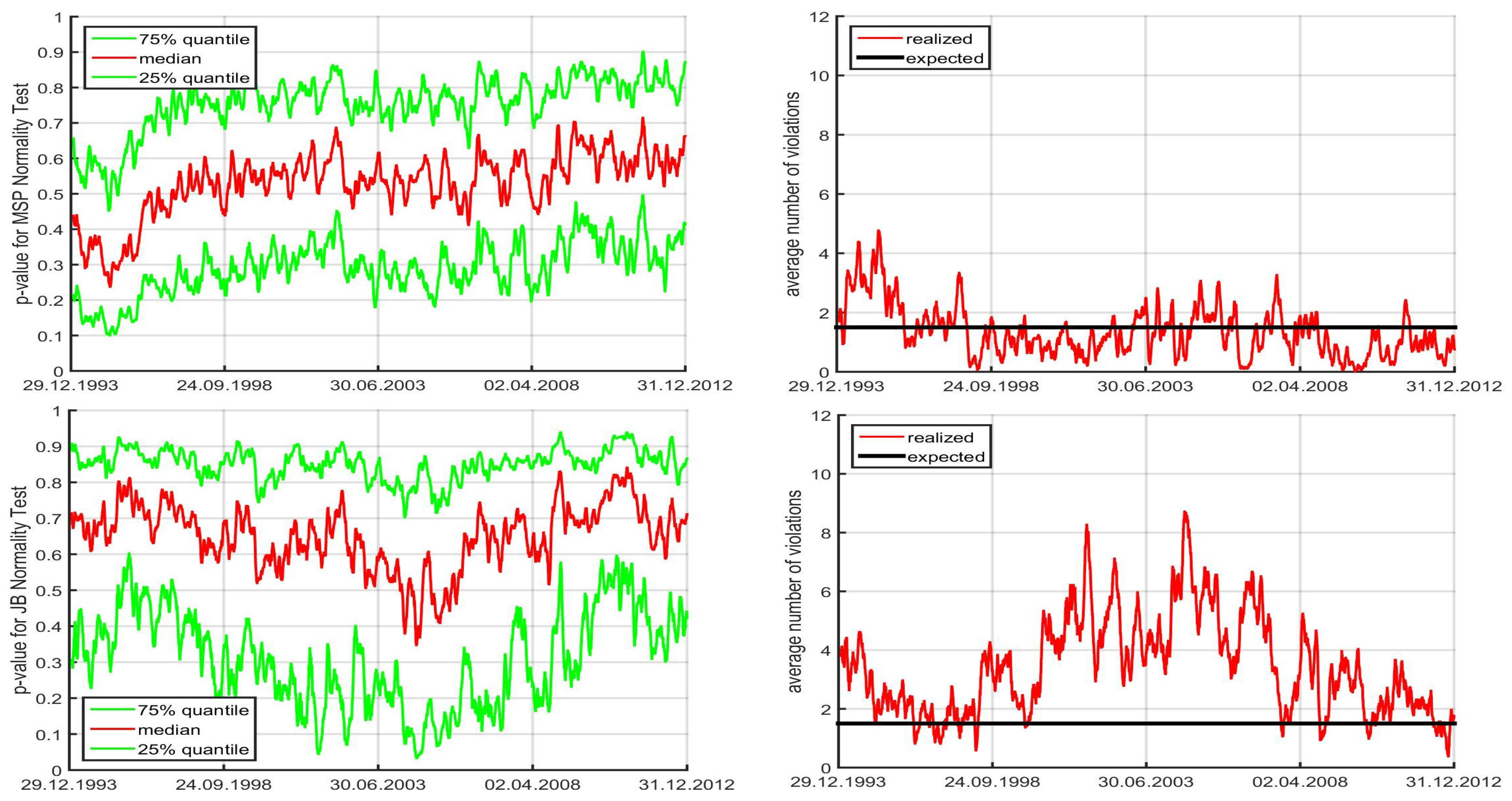
To help determine a possible set of alternative APARCH parameter values, Figure A4 shows the corresponding ML-estimated APARCH parameters , , and , through the same moving windows (with fixed value ). We see a significant change in the parameter estimates, notably , for the data segment corresponding to the “spiky” period shown in the top right panel of Figure A2. The right side of Figure A4 is just a magnified view of the problem region, and simple eye-balling gives rise to the following set of fixed model parameters:
Instead of casual inspection of the resulting estimated APARCH coefficients to specify the coefficients, it might be possible instead to optimize this. In particular, the coefficients could be chosen using particular windows of data that satisfy some criterion, in particular, we (somewhat arbitrarily) choose those for which the 75% quantile of the MSP test p-values, based on the initial KP-estimation results, falls below the threshold . There are 72 such windows. Label the resulting return sequences as , and let , , denote the p-value of the MSP test applied to the transformed filtered innovations of the fitted NCT-APARCH model with parameters , , and . We then estimate the APARCH parameters by minimizing MSP rejection probabilities,
using a specified tail probability , and is the indicator function. Observe that the objective function is not smooth, but rather integer-valued, and so, for optimization, we use the CMAES algorithm of Hansen and Ostermeier (2001).
Figure A4.
Quantiles, computed over 30 series, for the APARCH parameter estimates , , , over time, according to (6), based on rolling windows of size 250, with fixed value .
Figure A4.
Quantiles, computed over 30 series, for the APARCH parameter estimates , , , over time, according to (6), based on rolling windows of size 250, with fixed value .
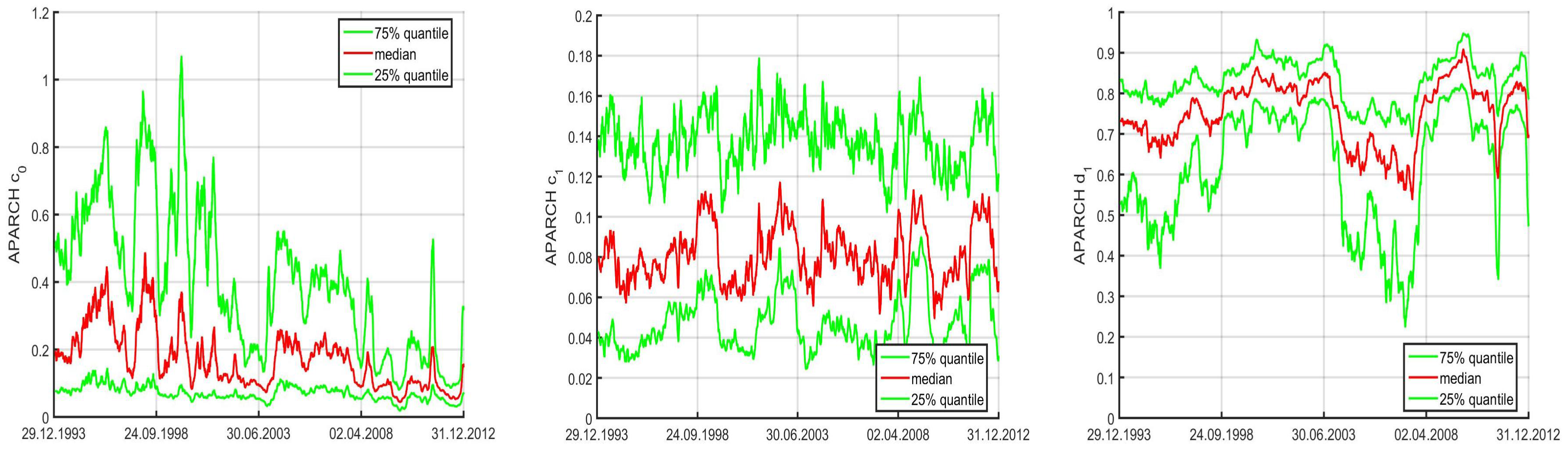
With , we obtain (to two significant digits, this being enough for practical application given the uncertainty of the parameters) , and , while using yields , and . Another objective function is maximizing MSP p-values towards , the expectation of the p-value under the null of the distribution,
yielding , and . Observe that all three optimization methods yield very similar point estimates for and , and those of are also rather close, but and differ substantially from those in (A2).
Based on this assessment, we consider the two APARCH formulations, (A2) and
and entertain the following APARCH-switching strategy for each univariate time series of returns: Use the baseline values (7) unless, based on them, either the MSP or Jarque-Bera p-value of the transformed-to-normality NCT-APARCH residuals are less than , where is now a tuning parameter that can be chosen based on out of sample portfolio performance.
Thus, there are two choices for the alternative APARCH specification, (A2) and (A5). The left and right panels of Figure A5 illustrate the performance of these, respectively, in terms of Sharpe ratio and total cumulative wealth, as a function of , having averaged the results over the eight stored runs used throughout the paper based on . The disappointing result emerges that this idea does not assist in delivering better-performing portfolios.
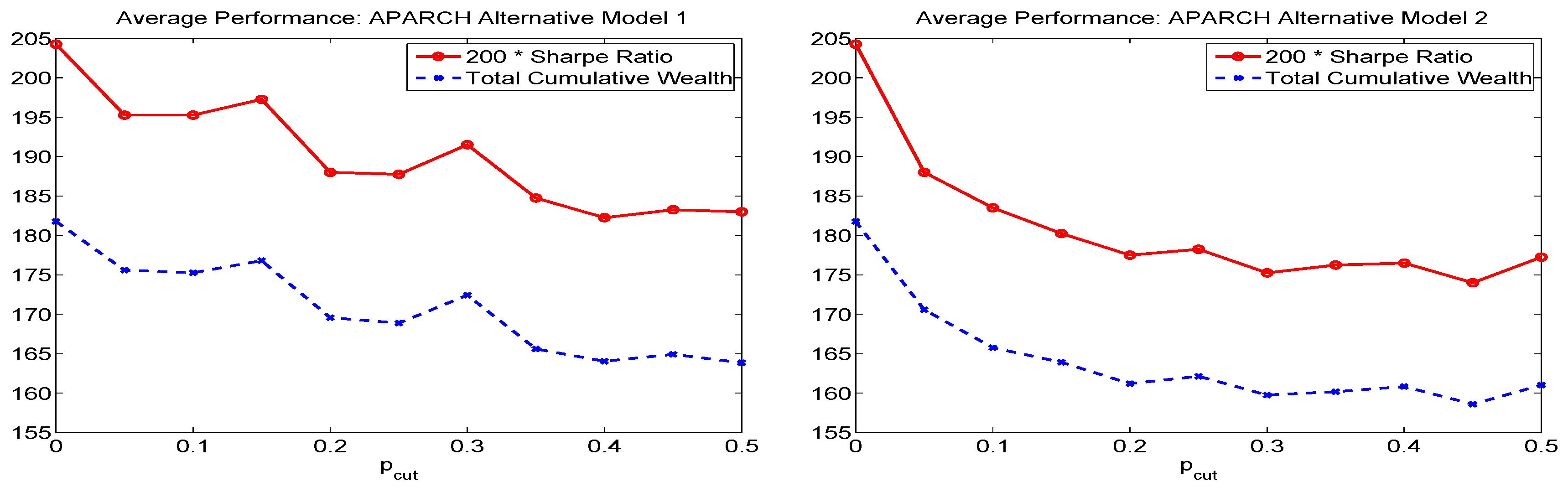
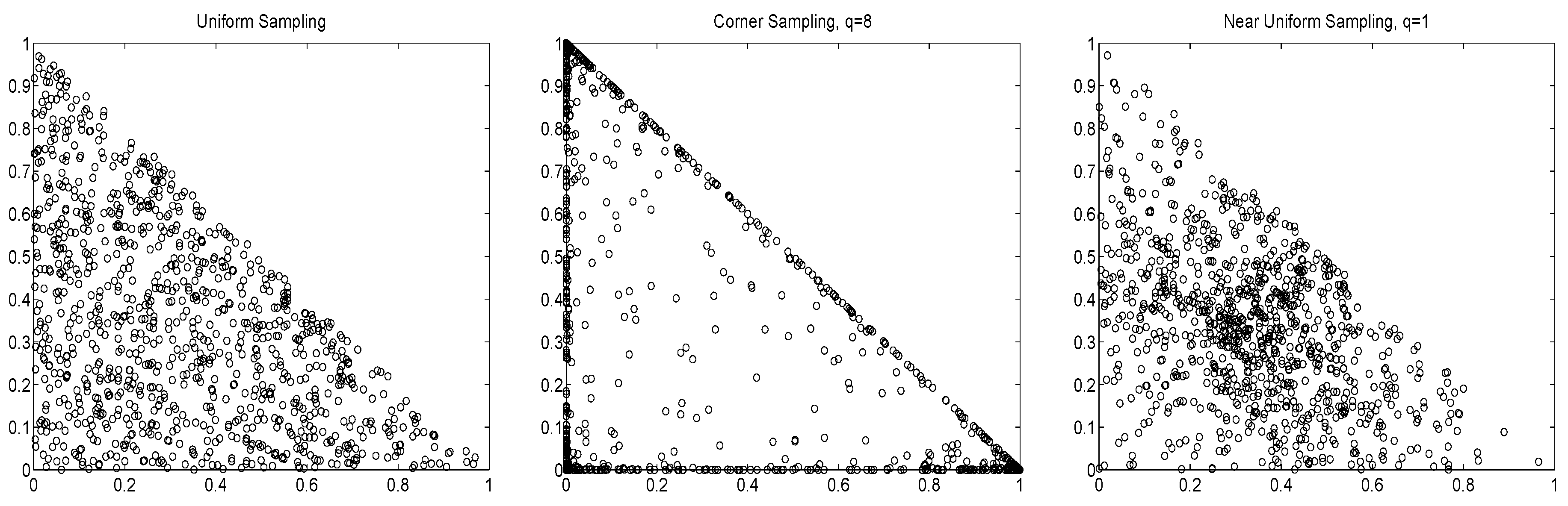
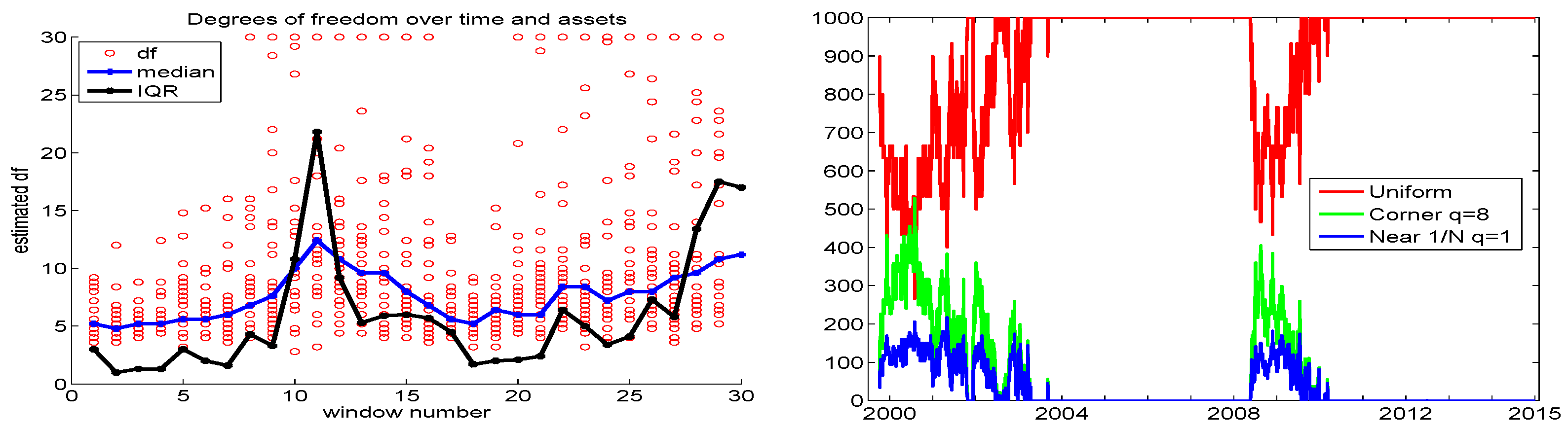
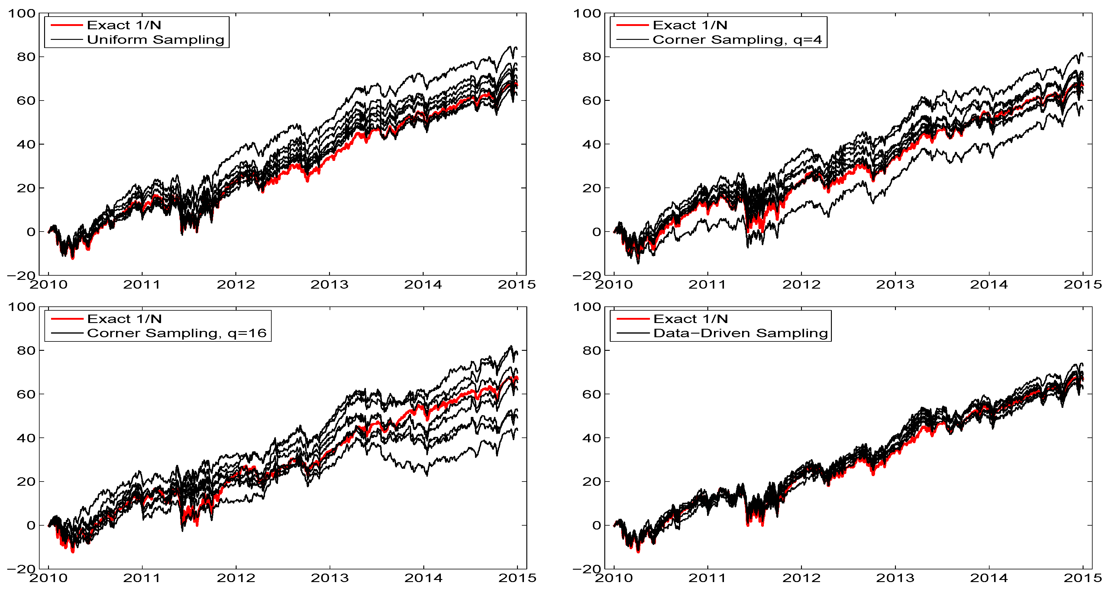
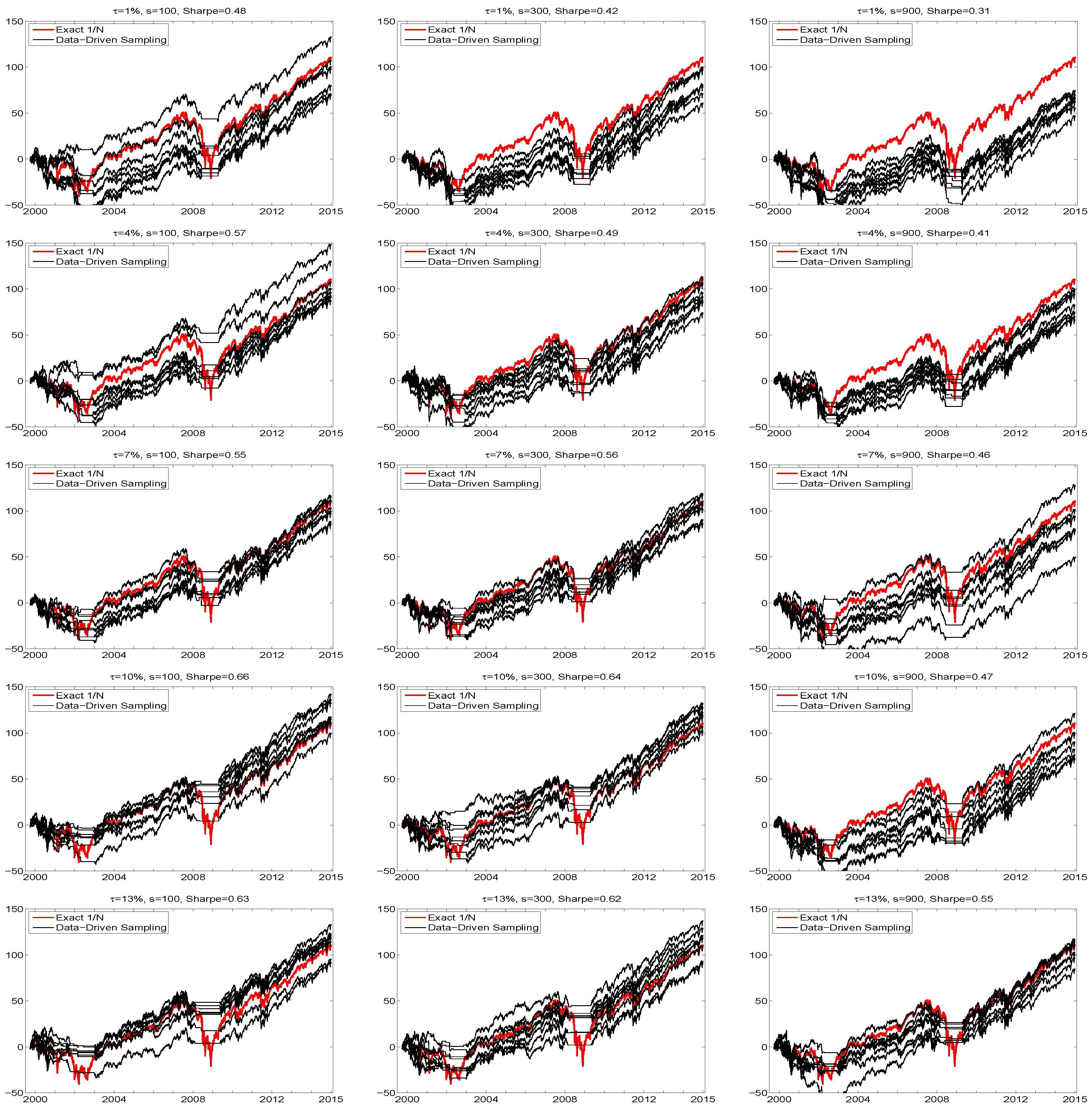
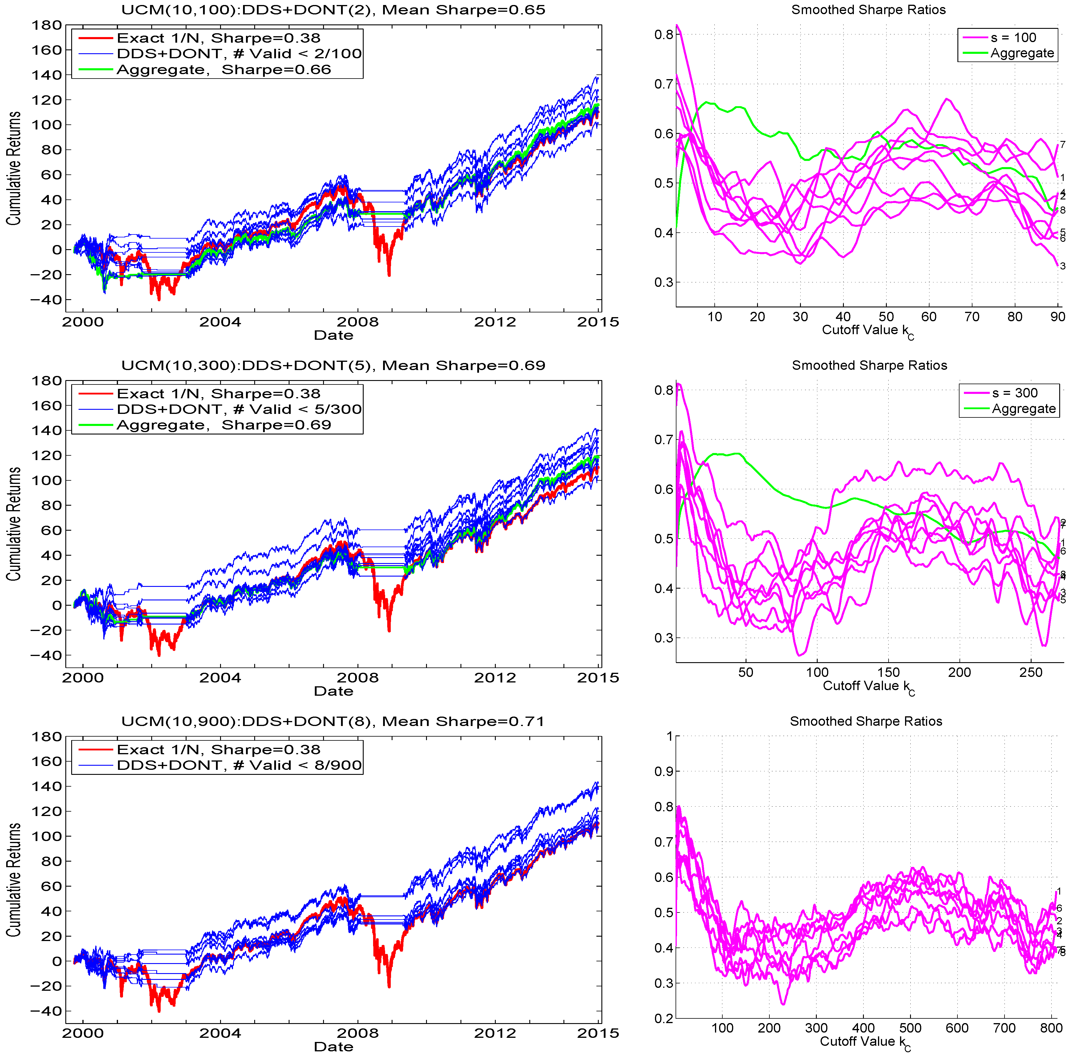
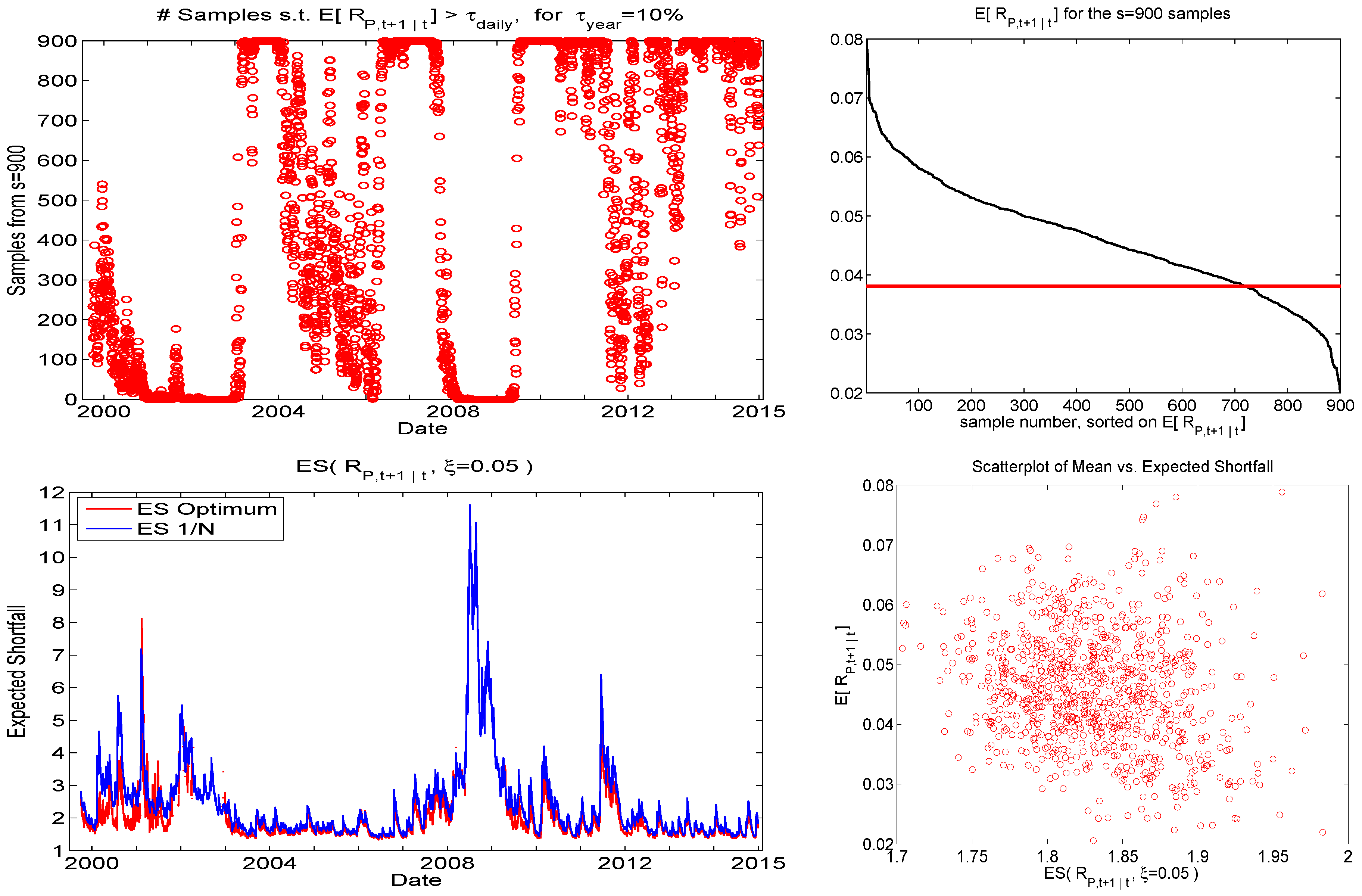
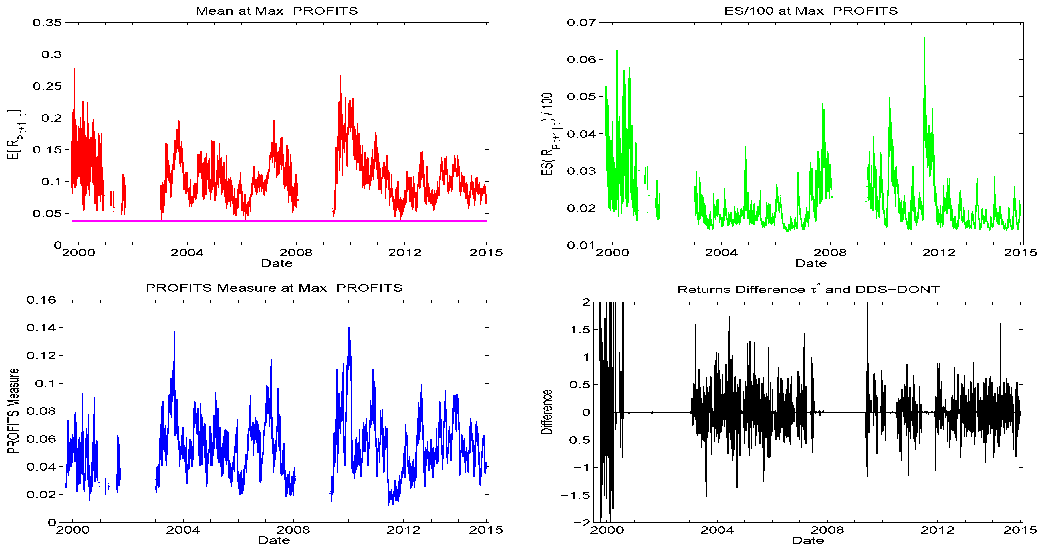
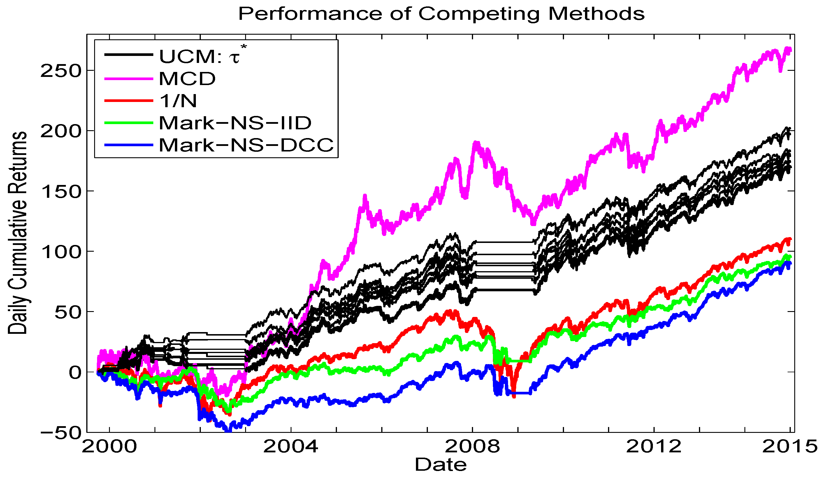
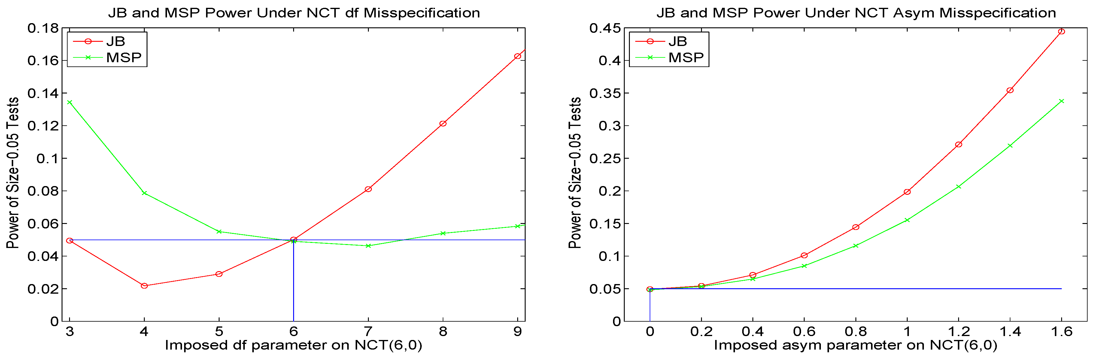
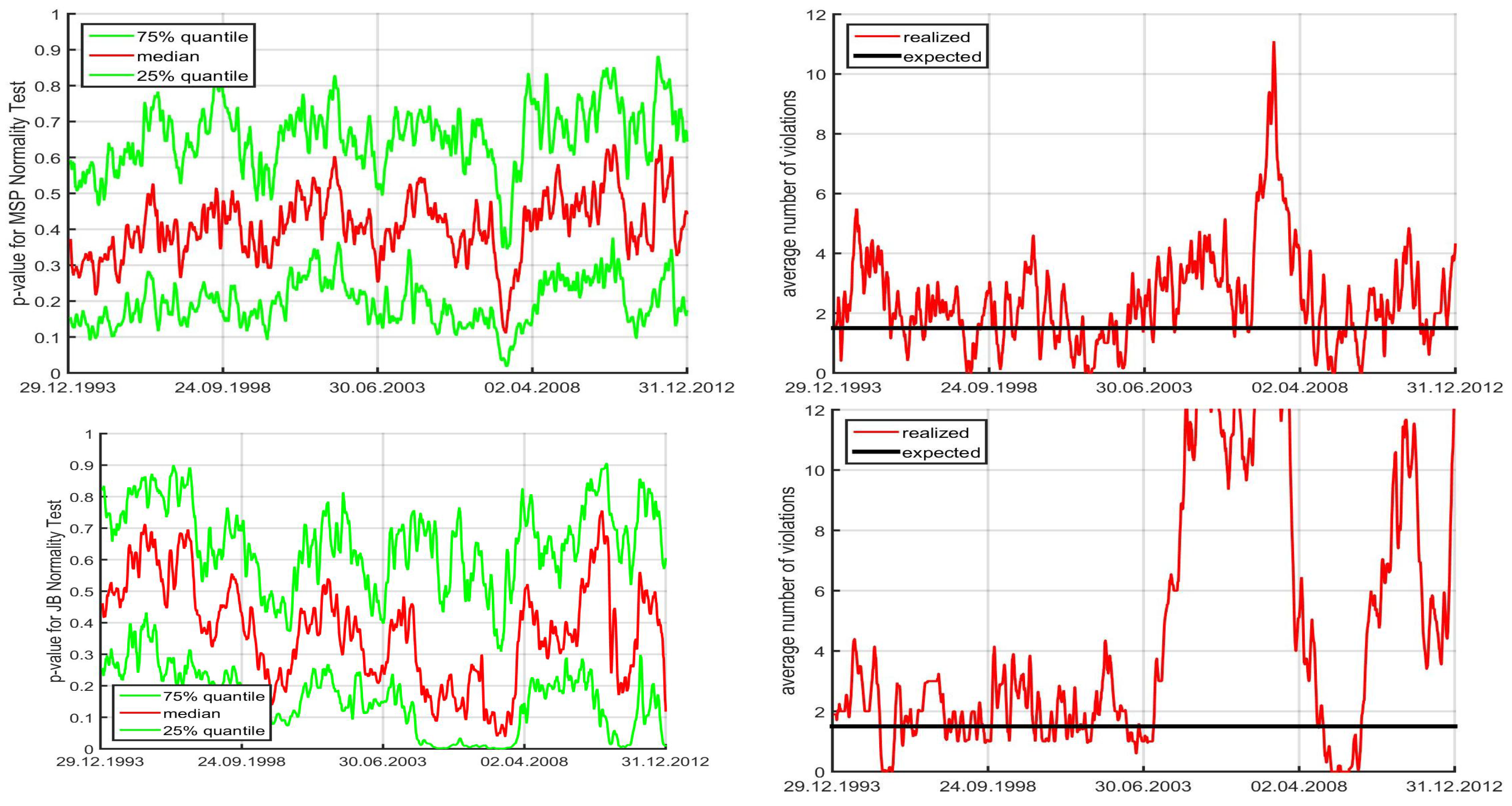
References
- Aas, Kjersti, Ingrid Hobæk Haff, and Xeni K. Dimakos. 2005. Risk Estimation using the Multivariate Normal Inverse Gaussian Distribution. Journal of Risk 8: 39–60. [Google Scholar] [CrossRef]
- Adcock, Christopher J. 2010. Asset Pricing and Portfolio Selection Based on the Multivariate Extended Skew-Student-t Distribution. Annals of Operations Research 176: 221–34. [Google Scholar] [CrossRef]
- Adcock, Christopher J. 2014. Mean—Variance—Skewness Efficient Surfaces, Stein’s Lemma and the Multivariate Extended Skew-Student Distribution. European Journal of Operational Research 234: 392–401. [Google Scholar] [CrossRef]
- Adcock, Christopher J., Martin Eling, and Nicola Loperfido. 2015. Skewed Distributions in Finance and Actuarial Science: A Preview. European Journal of Finance 21: 1253–81. [Google Scholar] [CrossRef]
- Allen, David E., Michael McAleer, Robert J. Powell, and Abhay K. Singh. 2016. Down-side Risk Metrics as Portfolio Diversification Strategies across the GFC. Journal of Risk and Financial Management 9: 6. [Google Scholar] [CrossRef]
- Andersen, Torben G., Tim Bollerslev, Peter F. Christoffersen, and Francis X. Diebold. 2007. Practical Volatility and Correlation Modeling for Financial Market Risk Management. In The Risks of Financial Institutions. Edited by Mark Carey and Rene M. Stulz. Chicago: The University of Chicago Press, chp. 11. pp. 513–44. [Google Scholar]
- Bauwens, Luc, Christian M. Hafner, and Jeroen V. K. Rombouts. 2007. Multivariate Mixed Normal Conditional Heteroskedasticity. Computational Statistics & Data Analysis 51: 3551–66. [Google Scholar] [CrossRef]
- Bauwens, Luc, Sébastien Laurent, and Jeroen V.K. Rombouts. 2006. Multivariate GARCH Models: A Survey. Journal of Applied Econometrics 21: 79–109. [Google Scholar] [CrossRef]
- Biglova, Almira, Sergio Ortobelli, Svetlozar Rachev, and Frank J. Fabozzi. 2010. Modeling, Estimation, and Optimization of Equity Portfolios with Heavy-Tailed Distributions. In Optimizing Optimization: The Next Generation of Optimization Applications and Theory. Edited by Stephen Satchell. Cambridge: Academic Press, pp. 117–42. [Google Scholar]
- Billio, Monica, Massimiliano Caporin, and Michele Gobbo. 2006. Flexible Dynamic Conditional Correlation Multivariate GARCH Models for Asset Allocation. Applied Financial Economics Letters 2: 123–30. [Google Scholar] [CrossRef]
- Bloomfield, Ted, Richard Leftwich, and John B. Long Jr. 1977. Portfolio Strategies and Performance. Journal of Financial Economics 5: 201–18. [Google Scholar] [CrossRef]
- Bollerslev, Tim. 1986. Generalized Autoregressive Conditional Heteroskedasticity. Journal of Econometrics 31: 307–27. [Google Scholar] [CrossRef]
- Bollerslev, Tim. 1990. Modeling the Coherence in Short-Run Nominal Exchange Rates: A Multivariate Generalized ARCH Approach. Review of Economics and Statistics 72: 498–505. [Google Scholar] [CrossRef]
- Bowman, K. O., and L. R. Shenton. 1975. Omnibus Test Contours for Departures from Normality Based on and b2. Biometrika 62: 243–50. [Google Scholar] [CrossRef]
- Brandt, Michael W., Pedro Santa-Clara, and Rossen Valkanov. 2009. Parametric Portfolio Policies: Exploiting Characteristics in the Cross-Section of Equity Returns. Review of Financial Studies 22: 3411–47. [Google Scholar] [CrossRef]
- Broda, Simon, and Marc S. Paolella. 2007. Saddlepoint Approximations for the Doubly Noncentral t Distribution. Computational Statistics & Data Analysis 51: 2907–18. [Google Scholar] [CrossRef]
- Broda, Simon A., Markus Haas, Jochen Krause, Marc S. Paolella, and Sven C. Steude. 2013. Stable Mixture GARCH Models. Journal of Econometrics 172: 292–306. [Google Scholar] [CrossRef]
- Broda, Simon A., and Marc S. Paolella. 2009. CHICAGO: A Fast and Accurate Method for Portfolio Risk Calculation. Journal of Financial Econometrics 7: 412–36. [Google Scholar] [CrossRef]
- Broda, Simon A., and Marc S. Paolella. 2011. Expected Shortfall for Distributions in Finance. In Statistical Tools for Finance and Insurance. Edited by Pavel Čížek, Wolfgang Härdle and Rafał Weron. Berlin: Springer Verlag, pp. 57–99. [Google Scholar]
- Brown, Stephen J., Inchang Hwang, and Francis In. 2013. Why Optimal Diversification Cannot Outperform Naive Diversification: Evidence from Tail Risk Exposure. Available online: https://www.researchgate.net/publication/273084879_Why_Optimal_Diversification_Cannot_Outperform_Naive_Diversification_Evidence_from_Tail_Risk_Exposure (accessed on 9 October 2016).
- Campbell, Rachel A., and Roman Kräussl. 2007. Revisiting the Home Bias Puzzle: Downside Equity Risk. Journal of International Money and Finance 26: 1239–60. [Google Scholar] [CrossRef]
- Caporin, Massimiliano, and Michael McAleer. 2008. Scalar BEKK and Indirect DCC. Journal of Forecasting 27: 537–49. [Google Scholar] [CrossRef]
- Caporin, Massimiliano, and Michael McAleer. 2012. Do We Really Need Both BEKK and DCC? A Tale of Two Multivariate GARCH Models. Journal of Economic Surveys 26: 736–51. [Google Scholar] [CrossRef]
- Cappiello, Lorenzo, Robert F. Engle, and Kevin Sheppard. 2006. Asymmetric Dynamics in the Correlations of Global Equity and Bond Returns. Journal of Financial Econometrics 4: 537–72. [Google Scholar] [CrossRef]
- Chopra, Vijay Kumar, and William T. Ziemba. 1993. The Effect of Errors in Means, Variances, and Covariances on Optimal Portfolio Choice. Journal of Portfolio Management 19: 6–11. [Google Scholar] [CrossRef]
- Christoffersen, Peter. 2009. Value-at-Risk Models. In Handbook of Financial Time Series. Edited by Thomas Mikosch, Jens-Peter Kreiss, Richard A. Davis and Torben Gustav Andersen. Berlin: Springer-Verlag, pp. 753–66. [Google Scholar]
- Cogneau, Philippe, and Georges Hübner. 2009a. The (more than) 100 Ways to Measure Portfolio Performance—Part 1: Standardized Risk-Adjusted Measures. Journal of Performance Measurement 13: 56–71. [Google Scholar]
- Cogneau, Philippe, and Georges Hübner. 2009b. The (more than) 100 Ways to Measure Portfolio Performance—Part 2: Special Measures and Comparison. Journal of Performance Measurement 14: 56–69. [Google Scholar]
- D’Agostino, Ralph, and E. S. Pearson. 1973. Testing for Departures from Normality. Empirical Results for Distribution of b2 and . Biometrika 60: 613–22. [Google Scholar]
- Davis, Mark H. A. 2016. Verification of Internal Risk Measure Estimates. Statistics and Risk Modeling, 33. [Google Scholar] [CrossRef]
- DeMiguel, Victor, Lorenzo Garlappi, Francisco J. Nogales, and Raman Uppal. 2009a. A Generalized Approach to Portfolio Optimization: Improving Performance by Constraining Portfolio Norms. Management Science 55: 798–812. [Google Scholar] [CrossRef]
- DeMiguel, Victor, Lorenzo Garlappi, and Raman Uppal. 2009b. Optimal Versus Naive Diversification: How Inefficient is the 1/N Portfolio Strategy? Review of Financial Studies 22: 1915–53. [Google Scholar] [CrossRef]
- Diebold, Francis X., Todd A. Gunther, and Anthony S. Tay. 1998. Evaluating Density Forecasts with Applications to Financial Risk Management. International Economic Review 39: 863–83. [Google Scholar] [CrossRef]
- Ding, Zhuanxin, Clive W. J. Granger, and Robert F. Engle. 1993. A Long Memory Property of Stock Market Returns and a New Model. Journal of Empirical Finance 1: 83–106. [Google Scholar] [CrossRef]
- Embrechts, Paul, and Marius Hofert. 2014. Statistics and Quantitative Risk Management for Banking and Insurance. Annual Review of Statistics and Its Application 1: 493–514. [Google Scholar] [CrossRef]
- Embrechts, Paul, Alexander McNeil, and Daniel Straumann. 2002. Correlation and Dependency in Risk Management: Properties and Pitfalls. In Risk Management: Value at Risk and Beyond. Edited by M. A. H. Dempster. Cambridge: Cambridge University Press, pp. 176–223. [Google Scholar]
- Engle, Robert F. 2002. Dynamic Conditional Correlation: A Simple Class of Multivariate Generalized Autoregressive Conditional Heteroskedasticity Models. Journal of Business and Economic Statistics 20: 339–50. [Google Scholar]
- Engle, Robert F. 2009. Anticipating Correlations: A New Paradigm for Risk Management. Princeton: Princeton University Press. [Google Scholar]
- Engle, Robert F., and Kenneth F. Kroner. 1995. Multivariate Simultaneous Generalized ARCH. Econometric Theory 11: 122–50. [Google Scholar] [CrossRef]
- Fama, Eugene F., and Kenneth R. French. 1993. Common Risk Factors in the Returns of Stocks and Bonds. Journal of Financial Economics 33: 3–56. [Google Scholar] [CrossRef]
- Fama, Eugene F., and Kenneth R. French. 1996. Multifactor Explanations of Asset Pricing Anomalies. Journal of Finance 51: 55–84. [Google Scholar]
- Fletcher, Jonathan. 2017. Exploring the Benefits of Using Stock Characteristics in Optimal Portfolio Strategies. The European Journal of Finance 23: 192–210. [Google Scholar] [CrossRef]
- Francq, Christian, and Jean-Michel Zakoïan. 2010. GARCH Models: Structure, Statistical Inference and Financial Applications. Hoboken: John Wiley & Sons Ltd. [Google Scholar]
- Fugazza, Carolina, Massimo Guidolin, and Giovanna Nicodano. 2015. Equally Weighted vs. Long-Run Optimal Portfolios. European Financial Management 21: 742–89. [Google Scholar] [CrossRef]
- Gambacciani, Marco, and Marc S. Paolella. 2017. Robust Normal Mixtures for Financial Portfolio Allocation. Econometrics and Statistics. [Google Scholar] [CrossRef]
- Glosten, Lawrence R., Ravi Jagannathan, and David E. Runkle. 1993. On the Relation between the Expected Value and Volatility of Nominal Excess Return on Stocks. Journal of Finance 48: 1779–801. [Google Scholar] [CrossRef]
- Haas, Markus, Stefan Mittnik, and Marc S. Paolella. 2009. Asymmetric Multivariate Normal Mixture GARCH. Computational Statistics & Data Analysis 53: 2129–54. [Google Scholar] [CrossRef]
- Hansen, Nikolaus, and Andreas Ostermeier. 2001. Completely Derandomized Self-Adaptation in Evolution Strategies. Evolutionary Computation 9: 159–95. [Google Scholar] [CrossRef] [PubMed]
- Härdle, Wolfgang Karl, Ostap Okhrin, and Weining Wang. 2015. Hidden Markov Structures for Dynamic Copulae. Econometric Theory 31: 981–1015. [Google Scholar] [CrossRef]
- He, Changli, and Timo Teräsvirta. 1999. Statistical Properties of the Asymmetric Power ARCH Model. In Cointegration, Causality, and Forecasting. Festschrift in Honour of Clive W. J. Granger. Edited by Robert F. Engle and Halbert White. Oxford: Oxford University Press, pp. 462–474. [Google Scholar]
- Jagannathan, Ravi, and Tongshu Ma. 2003. Risk Reduction in Large Portfolios: Why Imposing the Wrong Constraints Helps. Journal of Finance 58: 1651–84. [Google Scholar] [CrossRef]
- Jarque, Carlos M., and Anil K. Bera. 1980. Efficient Tests for Normality, Homoskedasticity and Serial Independence of Regression Residuals. Economics Letters 6: 255–59. [Google Scholar] [CrossRef]
- Jondeau, Eric. 2016. Asymmetry in Tail Dependence of Equity Portfolios. Computational Statistics & Data Analysis 100: 351–68. [Google Scholar] [CrossRef]
- Jondeau, Eric, Ser-Huang Poon, and Michael Rockinger. 2007. Financial Modeling Under Non-Gaussian Distributions. London: Springer. [Google Scholar]
- Jorion, Philippe. 1986. Bayes-Stein Estimation for Portfolio Analysis. Journal of Financial and Quantitative Analysis 21: 279–92. [Google Scholar] [CrossRef]
- Kan, Raymond, and Guofu Zhou. 2007. Optimal Portfolio Choice with Parameter Uncertainty. Journal of Financial and Quantitative Analysis 42: 621–56. [Google Scholar] [CrossRef]
- Karanasos, Menelaos, and Jinki Kim. 2006. A Re-Examination of the Asymmetric Power ARCH Model. Journal of Empirical Finance 13: 113–28. [Google Scholar] [CrossRef]
- Krause, Jochen, and Marc S. Paolella. 2014. A Fast, Accurate Method for Value at Risk and Expected Shortfall. Econometrics 2: 98–122. [Google Scholar] [CrossRef]
- Kuester, Keith, Stefan Mittnik, and Marc S. Paolella. 2006. Value–at–Risk Prediction: A Comparison of Alternative Strategies. Journal of Financial Econometrics 4: 53–89. [Google Scholar] [CrossRef]
- Ledoit, Olivier, and Michael Wolf. 2004. Honey, I Shrunk the Sample Covariance Matrix. Journal of Portfolio Management 30: 110–19. [Google Scholar] [CrossRef]
- Ledoit, Oliver, and Michael Wolf. 2008. Robust Performance Hypothesis Testing with the Sharpe Ratio. Journal of Empirical Finance 15: 850–59. [Google Scholar] [CrossRef]
- Ledoit, Olivier, and Michael Wolf. 2012. Nonlinear Shrinkage Estimation of Large-Dimensional Covariance Matrices. Annals of Statistics 40: 1024–60. [Google Scholar] [CrossRef]
- Lehmann, E. L., and George Casella. 1998. Theory of Point Estimation, 2nd ed. New York: Springer Verlag. [Google Scholar]
- Ling, Shiqing, and Michael McAleer. 2002. Necessary and Sufficient Moment Conditions for the GARCH(r, s) and Asymmetric Power GARCH(r, s) Models. Econometric Theory 18: 722–29. [Google Scholar] [CrossRef]
- Lo, Andrew W. 2002. The Statistics of Sharpe Ratios. Financial Analysts Journal 58: 36–52. [Google Scholar] [CrossRef]
- Manganelli, Simone. 2004. Asset Allocation by Variance Sensitivity. Journal of Financial Econometrics 2: 370–89. [Google Scholar] [CrossRef]
- McAleer, Michael, Felix Chan, Suhejla Hoti, and Offer Lieberman. 2008. Generalized Autoregressive Conditional Correlation. Econometric Theory 24: 1554–83. [Google Scholar] [CrossRef]
- McNeil, Alexander J., Rüdiger Frey, and Paul Embrechts. 2005. Quantitative Risk Management: Concepts, Techniques, and Tools. Princeton: Princeton University Press. [Google Scholar]
- Mittnik, Stefan, and Marc S. Paolella. 2000. Conditional Density and Value–at–Risk Prediction of Asian Currency Exchange Rates. Journal of Forecasting 19: 313–33. [Google Scholar] [CrossRef]
- Nadarajah, Saralees, Bo Zhang, and Stephen Chan. 2013. Estimation Methods for Expected Shortfall. Quantitative Finance 14: 271–91. [Google Scholar]
- Nijman, Theo, and Enrique Sentana. 1996. Marginalization and Contemporaneous Aggregation in Multivariate GARCH Processes. Journal of Econometrics 71: 71–87. [Google Scholar] [CrossRef]
- Paolella, Marc S. 2007. Intermediate Probability: A Computational Approach. Chichester: John Wiley & Sons. [Google Scholar]
- Paolella, Marc S. 2014. Fast Methods For Large-Scale Non-Elliptical Portfolio Optimization. Annals of Financial Economics 9, 02: 1440001. [Google Scholar] [CrossRef]
- Paolella, Marc S. 2015a. Multivariate Asset Return Prediction with Mixture Models. European Journal of Finance 21: 1214–52. [Google Scholar] [CrossRef]
- Paolella, Marc S. 2015b. New Graphical Methods and Test Statistics for Testing Composite Normality. Econometrics 3: 532–60. [Google Scholar] [CrossRef]
- Paolella, Marc S., and Paweł Polak. 2015a. ALRIGHT: Asymmetric LaRge-Scale (I)GARCH with Hetero-Tails. International Review of Economics and Finance 40: 282–97. [Google Scholar] [CrossRef]
- Paolella, Marc S., and Paweł Polak. 2015b. COMFORT: A Common Market Factor Non-Gaussian Returns Model. Journal of Econometrics 187: 593–605. [Google Scholar] [CrossRef]
- Paolella, Marc S., and Paweł Polak. 2015c. Density and Risk Prediction with Non-Gaussian COMFORT Models. Submitted for publication. [Google Scholar]
- Paolella, Marc S., and Paweł Polak. 2015d. Portfolio Selection with Active Risk Monitoring. Research paper. Zurich, Switzerland: Swiss Finance Institute. [Google Scholar]
- Paolella, Marc S., and Sven -C. Steude. 2008. Risk Prediction: A DWARF-like Approach. Journal of Risk Model Validation 2: 25–43. [Google Scholar]
- Santos, André A. P., Francisco J. Nogales, and Esther Ruiz. 2013. Comparing Univariate and Multivariate Models to Forecast Portfolio Value–at–Risk. Journal of Financial Econometrics 11, 2: 400–41. [Google Scholar] [CrossRef]
- Silvennoinen, Annastiina, and Timo Teräsvirta. 2009. Multivariate GARCH Models. In Handbook of Financial Time Series. Edited by Torben Gustav Andersen, Richard A. Davis, Jens-Peter Kreiss and Thomas Mikosch. Berlin: Springer Verlag, pp. 201–29. [Google Scholar]
- Sun, Pengfei, and Chen Zhou. 2014. Diagnosing the Distribution of GARCH Innovations. Journal of Empirical Finance 29: 287–303. [Google Scholar]
- Tunaru, Radu. 2015. Model Risk in Financial Markets: From Financial Engineering to Risk Management. Singapore: World Scientific. [Google Scholar]
- Virbickaite, Audrone, M. Concepción Ausín, and Pedro Galeano. 2016. A Bayesian Non-Parametric Approach to Asymmetric Dynamic Conditional Correlation Model with Application to Portfolio Selection. Computational Statistics & Data Analysis 100: 814–29. [Google Scholar] [CrossRef]
- Wu, Lei, Qingbin Meng, and Julio C. Velazquez. 2015. The Role of Multivariate Skew-Student Density in the Estimation of Stock Market Crashes. European Journal of Finance 21: 1144–60. [Google Scholar] [CrossRef]
- Zhu, Qiji Jim, David H. Bailey, Marcos Lopez de Prado, and Jonathan M. Borwein. 2017. The Probability of Backtest Overfitting. Journal of Computational Finance 20: 39–69. [Google Scholar]
Figure 1.
Scatterplot of the first two out of three portfolio weights, for different sampling schemes.
Figure 1.
Scatterplot of the first two out of three portfolio weights, for different sampling schemes.

Figure 2.
Left: Cumulative returns over the entire DJIA data, from 1 June 1999 to 31 December 2014, using the portfolio, and the indicated sampling methods, based on and window length of , so that the first trade occurs around June 2000. Right: Same, but with corner sampling, using the indicated values of exponent q.
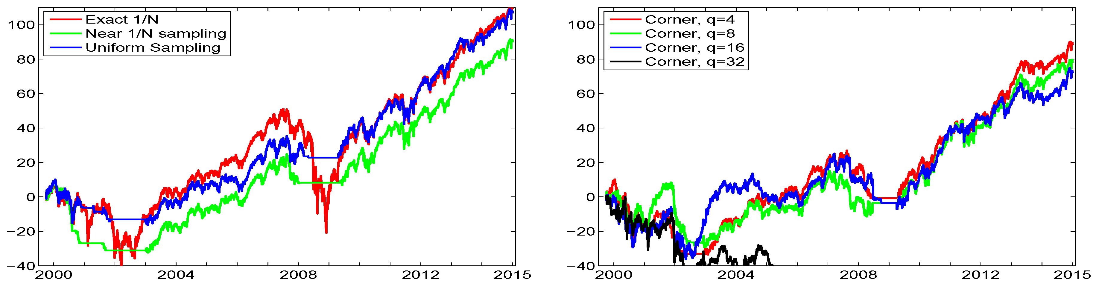
Figure 3.
Left: Cumulative return sequences of the DJIA data from 2009 to 2015 using the Markowitz iid long-only framework (denoted Mark-NS), based on moving windows of returns. The green line corresponds to the numerically optimized portfolio, while blue corresponds to use of the UCM method with uniform sampling, and replications. The result based on the equally weighted portfolio is also shown, in red. Right: Blue circles indicate the average, over all the windows, of , where and refer to the analytic (optimized) and UCM-based portfolio vectors, respectively. This was conducted times per sample size s for , and otherwise times. The red cross indicates the average over the h values.
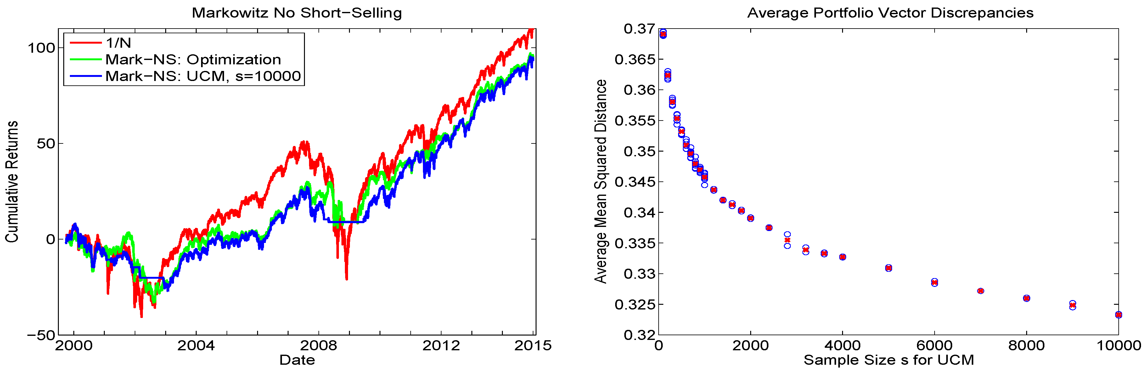
Figure 4.
Left: Circles show for each of the 29 assets, over 30 windows of length 250, for the 29 DJIA stocks, from 1 June 1999 to 31 December 2014. The blue (black) line shows their medians (IQR). Right: The resulting , and proportions (out of ), based on (14) and (15).
Figure 4.
Left: Circles show for each of the 29 assets, over 30 windows of length 250, for the 29 DJIA stocks, from 1 June 1999 to 31 December 2014. The blue (black) line shows their medians (IQR). Right: The resulting , and proportions (out of ), based on (14) and (15).

Figure 5.
Hair plots of eight cumulative return sequences, using the indicated method of sampling, of the DJIA data from 2009 to 2015 (so that the first trade occurs around January 2010), again with , , and . The thicker red line shows the exact performance. The bottom right panel corresponds to the data-driven sampling scheme (14) and (15) in Section 3.4.

Figure 6.
Hair plots, based on window size , of eight cumulative return sequences of the DJIA data (from June 1999 to December 2014), using data-driven sampling. The yearly percentage return, , and number of samples, s, are indicated in the titles, along with the attained annualized Sharpe ratio as the average over the eight sequences. The thicker red line shows the cumulative return performance of the equally weighted portfolio.

Figure 7.
Left: Similar exercise as shown in Figure 6, but only for , and using the cutoff strategy, such that, if out of the s samples, less than satisfy the mean constraint (as as indicated in the titles and legends), then trading is not conducted. Right: Smoothed Sharpe ratios for all runs, as a function of .

Figure 8.
For , left panels show the number of samples satisfying the mean constraint, and the predicted expected shortfall of the and optimal under DDS portfolios. The right panels plot the expected mean, sorted over the sampled portfolios, while the bottom panel shows a scatterplot of the predictive mean versus the predictive ES for the sampled portfolios, for time point t corresponding to the last observation in the data set.

Figure 9.
Left: Hair plot for , for the three indicated sampling sizes s, based on the same data as in the comparable plots in Figure 7, using the PROFITS technique and the optimal values of parameters and . Right: Obtained Sharpe ratios as a function of and , averaged over the eight runs, and smoothed, using a moving window of length two, for both dimensions, and for each of the three values of s.
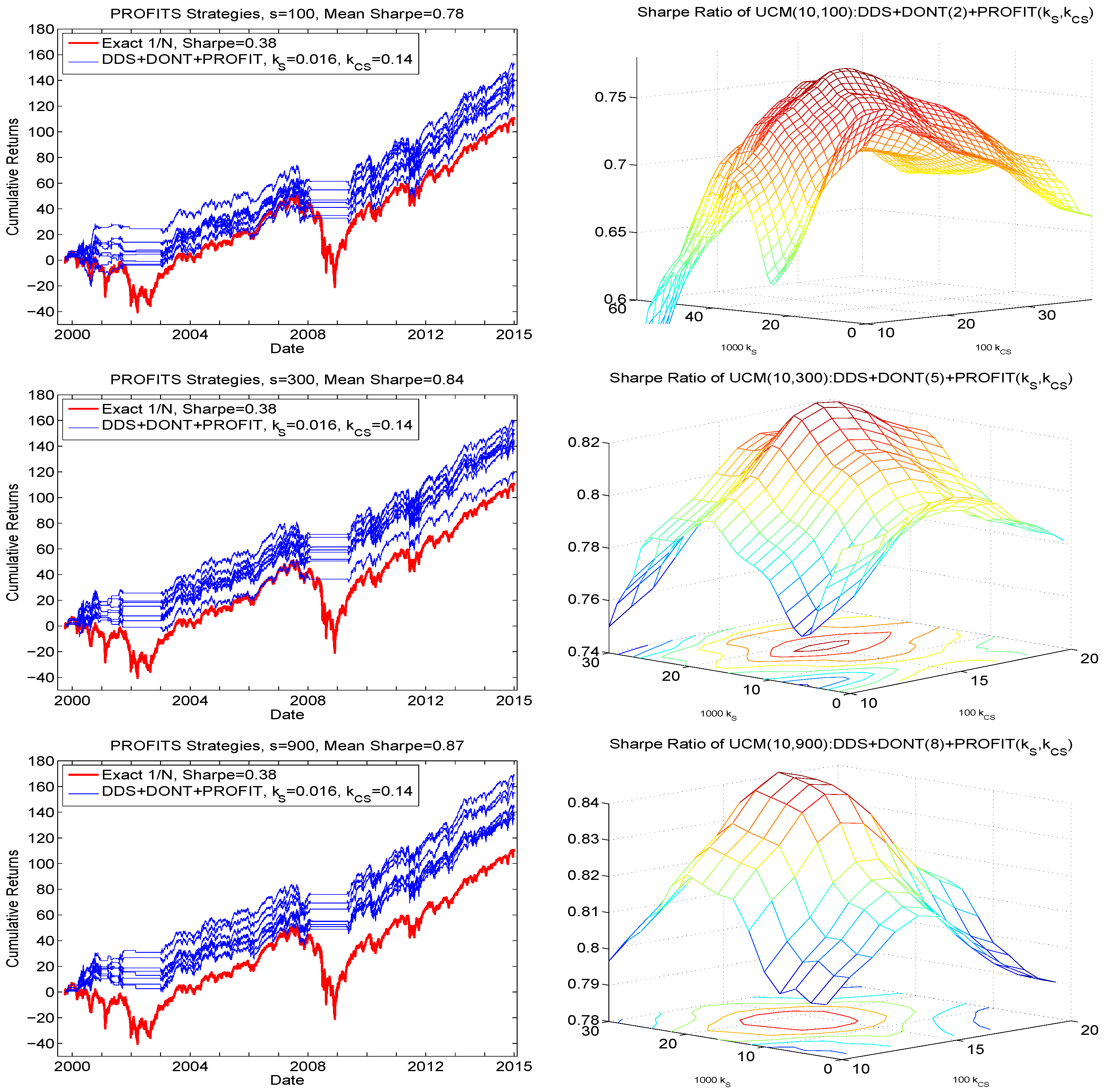
Figure 10.
Left: Hair plots for using the strategy, for . The same y-axis limits are used as throughout the paper for comparison purposes, and thus the upper values in the graphs corresponding to and have been truncated: For , the terminal wealth of the best of the eight runs reaches 201, while the average over the eight runs is 182. Right: Obtained Sharpe ratios as a function of , averaged over the eight runs, and smoothed.
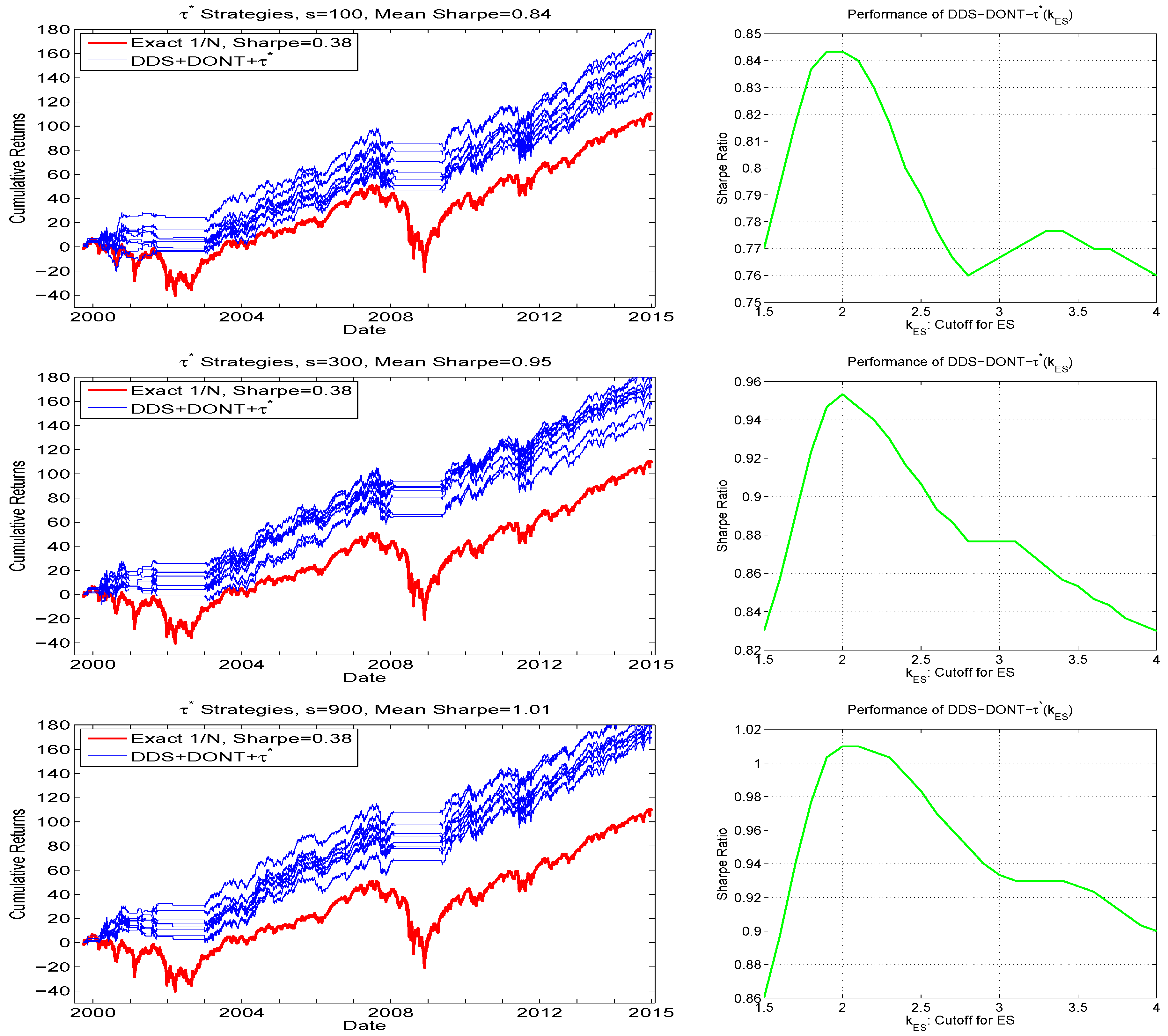
Figure 11.
Illustration, using , of the results from the method. It is based on the first of the eight conducted runs (they all result in very similar graphs). The graphs show the expected return, the predicted ES, the PROFITS measure, and the realized returns of DDS+DONT+ method minus those of DDS+DONT. The plot of ES divides by 100 simply to ensure that the top and bottom panels line up graphically via the spacing of the y-axis coordinates.

Figure 12.
Comparison of cumulative returns. Methods are: The UCM method based on 900 replications (same as in the lower left panel of Figure 10, black lines); Markowitz (no short selling) based on the iid assumption (green line) and using the Gaussian DCC-GARCH model (blue line) for computing the expected returns and their covariance matrix; the equally weighted method (red line); and based on an iid two-component mixed normal distribution with parameters estimated via the MCD methodology, from Gambacciani and Paolella (2017).

© 2017 by the author. Licensee MDPI, Basel, Switzerland. This article is an open access article distributed under the terms and conditions of the Creative Commons Attribution (CC BY) license (http://creativecommons.org/licenses/by/4.0/).
Share and Cite
MDPI and ACS Style
Paolella, M.S. The Univariate Collapsing Method for Portfolio Optimization. Econometrics 2017, 5, 18. https://doi.org/10.3390/econometrics5020018
AMA Style
Paolella MS. The Univariate Collapsing Method for Portfolio Optimization. Econometrics. 2017; 5(2):18. https://doi.org/10.3390/econometrics5020018
Chicago/Turabian StylePaolella, Marc S. 2017. "The Univariate Collapsing Method for Portfolio Optimization" Econometrics 5, no. 2: 18. https://doi.org/10.3390/econometrics5020018
Note that from the first issue of 2016, this journal uses article numbers instead of page numbers. See further details here.