Maximum Likelihood Estimation of the I(2) Model under Linear Restrictions

Abstract

Estimation of the I(2) cointegrated vector autoregressive (CVAR) model is considered. Without further restrictions, estimation of the I(1) model is by reduced-rank regression (Anderson (1951)). Maximum likelihood estimation of I(2) models, on the other hand, always requires iteration. This paper presents a new triangular representation of the I(2) model. This is the basis for a new estimation procedure of the unrestricted I(2) model, as well as the I(2) model with linear restrictions imposed.

1. Introduction

The I(1) model or cointegrated vector autoregression (CVAR) is now well established. The model is developed in a series of papers and books (see, e.g., Johansen (1988), Johansen (1991), Johansen (1995a), Juselius (2006)) and generally available in econometric software. The I(1) model is formulated as a rank reduction of the matrix of ‘long-run’ coefficients. The Gaussian log-likelihood is estimated by reduced-rank regression (RRR; see Anderson (1951), Anderson (2002)).

Determining the cointegrating rank only finds the cointegrating vectors up to a rank-preserving linear transformation. Therefore, the next step of an empirical study usually identifies the cointegrating vectors. This may be followed by imposing over-identifying restrictions. Common restrictions, i.e., the same restrictions on each cointegrating vector, can still be solved by adjusting the RRR estimation; see Johansen and Juselius (1990) and Johansen and Juselius (1992). Estimation with separate linear restrictions on the cointegrating vectors, or more general non-linear restrictions, requires iterative maximization. The usual approach is based on so-called switching algorithms; see Johansen (1995b) and Boswijk and Doornik (2004). The former proposes an algorithm that alternates between cointegrating vectors, estimating one while keeping the others fixed. The latter consider algorithms that alternate between the cointegrating vectors and their loadings: when one is kept fixed, the other is identified. The drawback is that these algorithms can be very slow and occasionally terminate prematurely. Doornik (2017) proposes improvements that can be applied to all switching algorithms.

Johansen (1995c) and Johansen (1997) extend the CVAR to allow for I(2) stochastic trends. These tend to be smoother than I(1) stochastic trends. The I(2) model implies a second reduced rank restriction, but this is now more complicated, and estimation under Gaussian errors can no longer be performed by RRR. The basis of an algorithm for maximum likelihood estimation is presented in Johansen (1997), with an implementation in Dennis and Juselius (2004).

The general approach to handling the I(2) model is to create representations that introduce parameters that vary freely without changing the nature of the model. This facilitates both the statistical analysis and the estimation.

The contributions of the current paper are two-fold. First, we present the triangular representation of the I(2) model. This is a new trilinear formulation with a block-triangular matrix structure at its core. The triangular representation provides a convenient framework for imposing linear restrictions on the model parameters. Next, we introduce several improved estimation algorithms for the I(2) model. A simulation experiment is used to study the behaviour of the algorithms.

Notation

Let $\alpha$ ($p\times r$) be a matrix with full column rank $r,r\le p$. The perpendicular matrix ${\alpha }_{∟}$ ($p\times p-r$) has ${\alpha }_{∟}^{\prime }\alpha =0$. The orthogonal complement ${\alpha }_{\perp }$ has ${\alpha }_{\perp }^{\prime }\alpha =0$ with the additional property that ${\alpha }_{\perp }^{\prime }{\alpha }_{\perp }=I_{p-r}$. Define $\tilde{\alpha }=\alpha {\left({\alpha }^{\prime }\alpha \right)}^{-1/2}$ and $\overline{\alpha }=\alpha {\left({\alpha }^{\prime }\alpha \right)}^{-1}$. Then, $(\tilde{\alpha }:{\alpha }_{\perp })$ is a $p\times p$ orthogonal matrix, so $I_p=\tilde{\alpha }{\tilde{\alpha }}^{\prime }+{\alpha }_{\perp }{\alpha }_{\perp }^{\prime }=\overline{\alpha }{\alpha }^{\prime }+{\alpha }_{\perp }{\alpha }_{\perp }^{\prime }=\alpha {\overline{\alpha }}^{\prime }+{\alpha }_{\perp }{\alpha }_{\perp }^{\prime }$.

The (thin) singular value decomposition (SVD) of $\alpha$ is $\alpha =UW{V}^{\prime }$, where $U(p\times r),V(r\times r)$ are orthogonal: $U^{\prime }U=V^{\prime }V=V{V}^{\prime }=I_r$, and W is a diagonal matrix with the ordered positive singular values on the diagonal. If rank$\left(\alpha \right)=s<r$, then the last $r-s$ singular values are zero. We can find ${\alpha }_{\perp }=U_2$ from the SVD of the square matrix $(\alpha :0)=(U_1:U_2)W{V}^{\prime }=(U_1{W}_1{V}_1^{\prime }:0)$.

The (thin) QR factorization of $\alpha$ with pivoting is $\alpha P=QR$, with $Q(p\times r)$ orthogonal and R upper triangular. This pivoting is the reordering of columns of $\alpha$ to better handle poor conditioning and singularity, and is captured in P, as discussed Golub and Van Loan (2013, §5.4.2).

The QL decomposition of A can be derived from the QR decomposition of $JAJ$: $JAJ=QR$, so $A=JJAJJ=JQJJZJ=Q^{\prime }L$. J is the exchange matrix, which is the identity matrix with columns in reverse order: premultiplication reverses rows; postmultiplication reverses columns; and $JJ=I$.

Let $\overline{\overline{\alpha }}={\Omega }^{-1}\alpha {\left({\alpha }^{\prime }{\Omega }^{-1}\alpha \right)}^{-1}$, then ${\alpha }_{\perp }^{\prime }\Omega \overline{\overline{\alpha }}=0$.

Finally, $a\leftarrow b$ assigns the value of b to a.

2. The I(2) Model

The vector autoregression (VAR) with p dependent variables and $m\ge 1$ lags:

$$y_t=A_1{y}_{t-1}+...+A_m{y}_{t-m}+\Phi x_t^U+{ϵ}_t,{ϵ}_t\sim {\mathrm{IIN}}_p[0_p,\Omega ],$$

for $t=1,...,T$, and with $y_j,j=-m+1,...,0$ fixed and given, can be written in equilibrium correction form as:

$$\Delta y_t={\Pi }_y{y}_{t-1}+{\Gamma }_1\Delta y_{t-1}+...+{\Gamma }_{m-1}\Delta y_{t-m+1}+\Phi x_t^U+{ϵ}_t,$$

without imposing any restrictions. The I(1) cointegrated VAR (CVAR) imposes a reduced rank restriction on ${\Pi }_y(p\times p)$: rank${\Pi }_y=r$; see, e.g., Johansen and Juselius (1990), Johansen (1995a).

With $m\ge 2$, the model can be written in second-differenced equilibrium correction form as:

$${\Delta }^2{y}_t={\Pi }_y{y}_{t-1}-{\Gamma }_y\Delta y_{t-1}+{\Psi }_1{\Delta }^2{y}_{t-1}+...+{\Psi }_{m-2}{\Delta }^2{y}_{t-m+2}+\Phi x_t^U+{ϵ}_t.$$

(1)

The I(2) CVAR involves an additional reduced rank restriction:

$$\begin{array}{cc}\hfill \mathrm{rank}\left({\alpha }_{\perp }^{\prime }{\Gamma }_y{\beta }_{y,\perp }\right)& =s,\hfill \end{array}$$

where ${\alpha }_{\perp }^{\prime }\alpha =0.$ The two rank restrictions can be expressed more conveniently in terms of products of matrices with reduced dimensions:

$$\begin{array}{cc}\hfill {\Pi }_y& =\alpha {\beta }_y^{\prime },\hfill \end{array}$$

(2)

$$\begin{array}{cc}\hfill {\alpha }_{\perp }^{\prime }{\Gamma }_y{\beta }_{y,\perp }& =\xi {\eta }_y^{\prime },\hfill \end{array}$$

(3)

where $\alpha$ and ${\beta }_y$ are $p\times r$ matrices. The second restriction needs rank s, so $\xi$ and ${\eta }_y$ are a $(p-r)\times s$. This requires that the matrices on the right-hand side of (2) and (3) have full column rank. The number of I(2) trends is $s_2=p-r-s$.

The most relevant model in terms of deterministics allows for linearly trending behaviour: $\Phi x_t^U={\mu }_0+{\mu }_{1}t$ . Using the representation theorem of Johansen (1992) and assuming $\mathsf{E}\left[y_t\right]=a+bt$ imply:

$$\begin{array}{cc}\hfill {\mu }_1& =-\alpha {\beta }_y^{\prime }b,\hfill \end{array}$$

(4)

$$\begin{array}{cc}\hfill {\mu }_0& =-\alpha {\beta }_y^{\prime }a+{\Gamma }_{y}b,\hfill \end{array}$$

(5)

which restricts and links ${\mu }_0$ and ${\mu }_1$; we see that ${\alpha }_{\perp }^{\prime }{\mu }_1=0$ and ${\alpha }_{\perp }^{\prime }{\mu }_0={\alpha }_{\perp }^{\prime }{\Gamma }_{y}b$.

2.1. The I(2) Model with a Linear Trend

The model (1) subject to the I(1) and I(2) rank restrictions (2) and (3) with $\Phi x_t^U={\mu }_0+{\mu }_{1}t$, subject to (4) and (5) can be written as:

$${\Delta }^2{y}_t=\alpha {\beta }^{\prime }\left(\begin{array}{c}{y}_{t-1}\\ t\end{array}\right)-\Gamma \left(\begin{array}{c}\Delta y_{t-1}\\ 1\end{array}\right)+{\Psi }_1{\Delta }^2{y}_{t-1}+...+{\Psi }_{m-2}{\Delta }^2{y}_{t-m+2}+{ϵ}_t,$$

(6)

subject to:

$${\alpha }_{\perp }^{\prime }\Gamma {\beta }_{\perp }=\xi {\eta }^{\prime },$$

(7)

where $\beta$ is $p_1\times r$, $\Gamma$ is $p\times p_1$ and $\eta$ is $(p_1-r)\times s$. In this case, $p_1=p+1$. Because $\alpha$ is the leading term in (4), we can extend ${\beta }_y$ by introducing ${\beta }_c^{\prime }=-{\beta }_y^{\prime }b$, so ${\beta }^{\prime }=({\beta }_y^{\prime }:{\beta }_c^{\prime })$. Furthermore, $\Gamma$ has been extended to $\Gamma =({\Gamma }_y:{\Gamma }_c)=({\Gamma }_y:-{\mu }_0)$.

To see that (6) and (7) remains the same I(2) model, consider ${\alpha }_{\perp }^{\prime }{\Gamma }_c$ and insert $I_p={\beta }_y{\overline{\beta }}_y^{\prime }+{\beta }_{y\perp }{\beta }_{y\perp }^{\prime }$:

$$\begin{array}{cc}\hfill {\alpha }_{\perp }^{\prime }{\Gamma }_c& =-{\alpha }_{\perp }^{\prime }{\Gamma }_y{\overline{\beta }}_y{\beta }_y^{\prime }b-{\alpha }_{\perp }^{\prime }{\Gamma }_y{\beta }_{y\perp }{\beta }_{y\perp }^{\prime }b={\alpha }_{\perp }^{\prime }{\Gamma }_y{\overline{\beta }}_y{\beta }_c^{\prime }-\xi {\eta }_y^{\prime }{\beta }_{y\perp }^{\prime }b={\alpha }_{\perp }^{\prime }{\Gamma }_y{\overline{\beta }}_y{\beta }_c^{\prime }+\xi {\eta }_c^{\prime }.\hfill \end{array}$$

Using the perpendicular matrix:

$${\beta }_{{\displaystyle ∟}}=\left(\begin{array}{cc}{\beta }_{y\perp }& -{\overline{\beta }}_y{\beta }_c^{\prime }\\ 0& 1\end{array}\right)$$

we see that the rank condition is unaffected:

$${\alpha }_{\perp }^{\prime }\Gamma {\beta }_{{\displaystyle ∟}}=\left({\alpha }_{\perp }^{\prime }{\Gamma }_y{\beta }_{y\perp }:\xi {\eta }_c^{\prime }\right)=\left({\alpha }_{\perp }^{\prime }{\Gamma }_y{\beta }_{y\perp }:{\alpha }_{\perp }^{\prime }[-{\Gamma }_y{\overline{\beta }}_y{\beta }_c^{\prime }+{\Gamma }_c]\right)=\xi \left({\eta }_y^{\prime }:{\eta }_c^{\prime }\right).$$

A more general formulation allows for restricted deterministic and weakly exogenous variables $x_t^R$ and unrestricted variables $x_t^U$:

$$\begin{array}{cc}\hfill {\Delta }^2{y}_t& =\Pi \left(\begin{array}{c}{y}_{t-1}\\ x_{t-1}^R\end{array}\right)-\Gamma \left(\begin{array}{c}\Delta y_{t-1}\\ \Delta x_t^R\end{array}\right)+{\Psi }_1{\Delta }^2{y}_{t-1}+...+{\Psi }_{m-2}{\Delta }^2{y}_{t-m+2}+\Phi x_t^U+{ϵ}_t,\hfill \\ & =\Pi w_{2t}-\Gamma w_{1t}+\Psi w_{3t}+{ϵ}_t,\hfill \end{array}$$

where ${\Delta }^2{x}_t^R$, and its lags are contained in $x_t^U$; this in turn, is subsumed under $w_{3t}={({\Delta }^2{y}_{t-1}^{\prime },...,x_t^{U\prime })}^{\prime }$. The number of variables in $x_t^R$ is $p_1-p$, so $\Pi$ and $\Gamma$ always have the same dimensions. $\Psi$ is unrestricted, which allows it to be concentrated out by regressing all other variables on $w_{3t}$:

$$z_{0t}=\alpha {\beta }^{\prime }{z}_{2t}-\Gamma z_{1t}+{ϵ}_t,{ϵ}_t\sim {\mathrm{IIN}}_p[0_p,\Omega ].$$

(8)

To implement likelihood-ratio tests, it is necessary to count the number of restrictions:

$$\begin{array}{ccc}\mathrm{restrictions}\mathrm{on}\Pi :\hfill & \hfill (p-r)(p_1-r)& \mathrm{restrictions},\hfill \\ \mathrm{restrictions}\mathrm{on}\Gamma :\hfill & \hfill (p-r-s)(p_1-r-s)=s_2{s}_2^{*}& \mathrm{restrictions},\hfill \end{array}$$

defining $s_2^{*}=p_1-r-s$. The restrictions on $\Pi$ follow from the representation. Several representations of the I(2) model have been introduced in the literature to translate the implicit non-linear restriction (3) on $\Gamma$ into an explicit part of the model. These representations reveal the number of restrictions imposed on $\Gamma$, as is shown below.

First, we introduce the new triangular representation.

2.2. The Triangular Representation

Theorem 1.

Consider the model:

$$z_{0t}=\Pi z_{2t}-\Gamma z_{1t}+{ϵ}_t,$$

with rank restrictions $\Pi =\alpha {\beta }^{\prime }$ and ${\alpha }_{\perp }^{\prime }\Gamma {\beta }_{\perp }=\xi {\eta }^{\prime }$ where α is a $p\times r$ matrix, β is $p_1\times r$, ξ is $(p-r)\times s$, η is $(p_1-r)\times s$. This can be written as:

$$z_{0t}=AW{B}^{\prime }{z}_{2t}-AV{B}^{\prime }{z}_{1t}+{ϵ}_t,$$

(9)

where:

$$W=\left(\begin{array}{ccc}0& 0& 0\\ 0& 0& 0\\ W_{11}& 0& 0\end{array}\right),V=\left(\begin{array}{ccc}{V}_{31}& 0& 0\\ V_{21}& V_{22}& 0\\ V_{11}& V_{12}& V_{13}\end{array}\right).$$

(10)

$A,B,W_{11},V_{22}$ are full rank matrices. A is $p\times p$, and B is $p_1\times p_1$; moreover, A, B and the nonzero blocks in W and V are freely varying. A and B are partitioned as:

$$A=\left(A_2:A_1:A_0\right),B=\left(B_0:B_1:B_2\right),$$

where the blocks in A have $s_2,s,r$ columns respectively; for B, this is: $r,s,s_2^{*}$; $p_1=r+s+s_2^{*}$. W and V are partitioned accordingly.

Proof. 

Write $\tilde{\alpha }=\alpha {\left({\alpha }^{\prime }\alpha \right)}^{-1/2}$, such that ${\tilde{\alpha }}^{\prime }\tilde{\alpha }=I_r$. Construct A and B as:

$$A=\left({\alpha }_{\perp }{\xi }_{\perp }:{\alpha }_{\perp }\tilde{\xi }:\tilde{\alpha }\right),B=\left(\tilde{\beta }:{\beta }_{\perp }\tilde{\eta }:{\beta }_{\perp }{\eta }_{\perp }\right).$$

Now, $A^{\prime }A=I$ and $B^{\prime }B=I$. $A(p\times p)$ and $B(p_1\times p_1)$ are full rank by design. Define $V=A^{\prime }\Gamma B$:

$$V=\left(\begin{array}{ccc}{\xi }_{\perp }^{\prime }{\alpha }_{\perp }^{\prime }\Gamma \tilde{\beta }& {\xi }_{\perp }^{\prime }{\alpha }_{\perp }^{\prime }\Gamma {\beta }_{\perp }\tilde{\eta }& {\xi }_{\perp }^{\prime }{\alpha }_{\perp }^{\prime }\Gamma {\beta }_{\perp }{\eta }_{\perp }\\ {\tilde{\xi }}^{\prime }{\alpha }_{\perp }^{\prime }\Gamma \tilde{\beta }& {\tilde{\xi }}^{\prime }{\alpha }_{\perp }^{\prime }\Gamma {\beta }_{\perp }\tilde{\eta }& {\tilde{\xi }}^{\prime }{\alpha }_{\perp }^{\prime }\Gamma {\beta }_{\perp }{\eta }_{\perp }\\ {\tilde{\alpha }}^{\prime }\Gamma \tilde{\beta }& {\tilde{\alpha }}^{\prime }\Gamma {\beta }_{\perp }\tilde{\eta }& {\tilde{\alpha }}^{\prime }\Gamma {\beta }_{\perp }{\eta }_{\perp }\end{array}\right)=\left(\begin{array}{ccc}{V}_{31}& 0& 0\\ V_{21}& V_{22}& 0\\ V_{11}& V_{12}& V_{13}\end{array}\right).$$

$V_{22}={\left({\xi }^{\prime }\xi \right)}^{\frac{1}{2}}{\left({\eta }^{\prime }\eta \right)}^{\frac{1}{2}}$ is a full rank $s\times s$ matrix. The zero blocks in V arise because, e.g., ${\xi }_{\perp }^{\prime }{\alpha }_{\perp }^{\prime }\Gamma {\beta }_{\perp }={\xi }_{\perp }^{\prime }\xi {\eta }^{\prime }=0$. Trivially:

$$\Pi =\alpha {\beta }^{\prime }=A\left(\begin{array}{ccc}0& 0& 0\\ 0& 0& 0\\ W_{11}& 0& 0\end{array}\right)B^{\prime }=AW{B}^{\prime }.$$

$W_{11}={\left({\alpha }^{\prime }\alpha \right)}^{\frac{1}{2}}{\left({\beta }^{\prime }\beta \right)}^{\frac{1}{2}}$ is a full rank $r\times r$ matrix. Both W and V are $p\times p_1$ matrices. Because A and B are each orthogonal: $\Gamma =A{A}^{\prime }\Gamma B{B}^{\prime }=AV{B}^{\prime }.$

The QR decomposition shows that a full rank square matrix can be written as the product of an orthogonal matrix and a triangular matrix. Therefore, $AV{B}^{\prime }=A{L}_a{L}_a^{-1}V{L}_b{L}_b^{-1}{B}^{\prime }=A_{*}{V}_{*}{B}_{*}^{\prime }$ preserves the structure in $V_{*}$ when $L_a,L_b$ are lower triangular, as well as that in $W_{*}$. This shows that (9) holds for any full rank A and B, and the orthogonality can be relaxed.

Therefore, any model with full rank matrices A and B, together with any $W,V$ that have the zeros as described above, satisfies the I(2) rank restrictions. We obtain the same model by restricting A and B to be orthogonal. ☐

When $\Gamma$ is restricted only by the I(2) condition: rank$\Gamma =r+s+min(r,s_2)$. Then, V varies freely, except for the zero blocks, and the I(2) restrictions are imposed through the trilinear form of (9). $\Gamma =0$ implies $V=0$. Another way to have $s=0$ is $\Gamma =(\alpha :0)G$; in that case, $V\ne 0$.

The $s_2$ restrictions on the intercept (5) can be expressed as $A_2^{\prime }({\mu }_0-{\mu }_c)=0,$ using ${\mu }_c={\Gamma }_y{\overline{\beta }}_y{\beta }_c^{\prime }$, or ${\mu }_0=(A_1:A_0)v+{\mu }_c,$ for a vector v of length $r+s$.

2.3. Obtaining the Triangular Representation

The triangular representation shows that the I(2) model can be written in trilinear form:

$$z_{0t}=AW{B}^{\prime }{z}_{2t}-AV{B}^{\prime }{z}_{1t}+{ϵ}_t,$$

where A and B are freely varying, provided W and V have the appropriate structure.

Consider that we are given $\alpha ,\beta ,\Gamma$ of an I(2) CVAR with rank indices $r,s$ and wish to obtain the parameters of the triangular representation. First compute ${\alpha }_{\perp }^{\prime }\Gamma {\beta }_{\perp }=\xi {\eta }^{\prime }$, which can be done with the SVD, assuming rank s. From this, compute A and B:

$$A=(A_2:A_1:A_0)=\left({\alpha }_{\perp }{\xi }_{\perp }:{\alpha }_{\perp }\tilde{\xi }:\alpha \right),B=(B_0:B_1:B_2)=\left(\beta :{\beta }_{\perp }\tilde{\eta }:{\beta }_{\perp }{\eta }_{\perp }\right).$$

Then, $V=A^{-1}\Gamma B^{-1\prime }$. Because $\Gamma$ satisfies the I(2) rank restriction, V will have the corresponding block-triangular structure.

It may be of interest to consider which part of the structure can be retrieved in the case where rank$(\Pi )=r$, but rank$({\alpha }_{\perp }^{\prime }\Gamma {\beta }_{\perp })=p-r$, while it should be s. This would happen when using I(1) starting values for I(2) estimation. The off anti-diagonal blocks of zeros:

$$V^{*}=\left(\begin{array}{ccc}{V}_{31}^{*}& V_{32}^{*}& V_{33}^{*}\\ V_{21}& V_{22}& V_{23}^{*}\\ V_{11}& V_{12}& V_{13}^{*}\end{array}\right)\to \left(\begin{array}{ccc}{V}_{31}& 0& V_{33}\\ V_{21}& V_{22}& 0\\ V_{11}& V_{12}& V_{13}\end{array}\right)=V$$

(11)

can be implemented with two sweep operations:

$$\left(\begin{array}{ccc}{I}_{s_2}& -V_{32}^{*}{V}_{22}^{-1}& 0\\ 0& I_s& 0\\ 0& 0& I_r\end{array}\right)V^{*}\left(\begin{array}{ccc}{I}_r& 0& 0\\ 0& I_s& -V_{22}^{-1}{V}_{23}^{*}\\ 0& 0& I_{s_2^{*}}\end{array}\right).$$

The offsetting operations affect $A_1$ and $B_1$ only, so $\Pi$ and $\Gamma$ are unchanged. However, we cannot achieve $V_{33}=0$ in a similar way, because it would remove the zeros just obtained. The $V_{33}$ block has dimension $s_2{s}_2^{*}$ and represents the number of restrictions imposed on $\Gamma$ in the I(2) model. Similarly, the anti-diagonal block of zeros in W captures the restrictions on $\Pi$.

Note that the $r\times s_2^{*}$ block $V_{13}$ can be made lower triangular. Write the column partition of V as $(V_{·1}:V_{·2}:V_{·3})$, and use $V_{13}=LQ$ to replace $V_{·3}$ by $V_{·3}{Q}^{\prime }$ and $B_2$ by $B_2{Q}^{\prime }$. When $r<s_2^{*}$, the rightmost $s_2^{*}-r$ columns of L will be zero, and the corresponding columns of $B_2$ are not needed to compute $\Gamma$. This part can then be omitted from the likelihood evaluation. This is an issue when we propose an estimation procedure in §4.2.1.

2.4. Restoring Orthogonality

Although A and B are freely varying, interpretation may require orthogonality between column blocks. The column blocks of A are in reverse order from B to make V and W block lower triangular. As a consequence, multiplication of V or W from either side by a lower triangular matrix preserves their structure. This allows for the relaxation of the orthogonality of A and B, but also enables us to restore it again.

To restore orthogonality, let $\Gamma =A_{*}{V}_{*}{B}_{*}^{\prime }$, where $A_{*},B_{*}$ are not orthogonal, but with $V_{*}$ block-triangular. Now, use the QL decomposition to get $A_{*}=AL$, with A orthogonal and L lower triangular. Use the QR decomposition to get $B_{*}=BR$, with B orthogonal and R upper triangular. Then, $A_{*}{V}_{*}{B}_{*}^{\prime }=AL{V}_{*}{R}^{\prime }{B}^{\prime }=AV{B}^{\prime }$ with the blocks of zeros in V preserved. $A_{*}{W}_{*}{B}_{*}^{\prime }$ must be adjusted accordingly. When $\beta$ is restricted, $B_0$ cannot be modified like this. However, we can still adjust $(A_2:A_1)=A_{*}$ to get $A_{*}^{\prime }{A}_{*}=I_{p-r}$ and $A_0^{\prime }{A}_{*}=0$; with similar adjustments to $(B_1:B_2)$.

The orthogonal version is convenient mathematically, but for estimation, it is preferable to use the unrestricted version. We do not distinguish through notation, but the context will state when the orthogonal version is used.

2.5. Identification in the Triangular Representation

The matrices A and B are not identified without further restrictions. For example, rescaling $\alpha$ and $\beta$ as in $\alpha W_{11}{\beta }^{\prime }={\alpha }^{\prime }{c}^{-1}c{W}_{11}d{d}^{-1}\beta ={\alpha }^{*}c{W}_{11}d{\beta }^{*\prime }$ can be absorbed in V:

$$\left(\begin{array}{ccc}{V}_{31}d& 0& 0\\ V_{21}d& V_{22}& 0\\ c{V}_{11}d& c{V}_{12}& c{V}_{13}\end{array}\right).$$

When $\beta$ is identified, $W_{11}$ remains freely varying, and we can, e.g., set $c=W_{11}^{-1}$. However, it is convenient to transform to $W_{11}=I$, so that $A_0$ and $B_0$ correspond to $\alpha$ and $\beta$. This prevents part of the orthogonality, in the sense that $A_0^{\prime }{A}_0\ne I$ and $B_0^{\prime }{B}_0\ne I$.

The following scheme identifies A and B, under the assumption that $B_0$ is already identified through prior restrictions.

• Orthogonalize to obtain $A_0^{\prime }{A}_1=0,A_0^{\prime }{A}_2=0,A_1^{\prime }{A}_2=0$.
• Choose s full rank rows from $B_1$, denoted $M_{B_1}$, and set $B_1\leftarrow B_1{M}_{B_1}^{-1}$. Adjust V accordingly.
• Do the same for $B_2\leftarrow B_2{M}_{B_2}^{-1}$.
• Set $A_1\leftarrow A_1{V}_{22}$, $V_{21}\leftarrow V_{22}^{-1}{V}_{21}$ and $V_{22}\leftarrow I$.
• $A_2\leftarrow A_2{M}_{A_2}^{-1}$.

The ordering of columns inside $A_i,B_i$ is not unique.

3. Relation to Other Representations

Two other formulations of the I(2) model that are in use are the so-called $\tau$ and $\delta$ representations. All representations implement the same model and make the rank restrictions explicit. However, they differ in their definitions of freely-varying parameters, so may facilitate different forms of analysis, e.g., asymptotic analysis, estimation or the imposition of restrictions. The different parametrizations may also affect economic interpretations.

3.1. $\tau$ Representation

Johansen (1997) transforms (8) into the $\tau$-representation:

$$z_{0t}=\alpha \left({\varrho }^{\prime }{\tau }^{\prime }{z}_{2t}+{\psi }^{\prime }{z}_{1t}\right)+w{\kappa }^{\prime }{\tau }^{\prime }{z}_{1t}+{ϵ}_t,$$

(12)

where $\varrho (p_1\times r+s)$ is used to recover $\beta$: $\beta =\tau \varrho$. The parameters $(\alpha ,\varrho ,\tau ,\psi ,\kappa )$ vary freely. If we normalize on ${\varrho }^{\prime }=(I_r:0)$ and adjust $\kappa ,\tau$ accordingly, then $\tau =(\beta :{\beta }_1)$, and:

$$z_{0t}=\alpha \left({\beta }^{\prime }{z}_{2t}+{\psi }^{\prime }{z}_{1t}\right)+w{\kappa }^{\prime }{\tau }^{\prime }{z}_{1t}+{ϵ}_t.$$

We shall derive the $\tau$ representation. The first step is to define a transformation of ${ϵ}_t\sim \mathrm{N}[0,\Omega ]$:

$${\left(\begin{array}{cc}{\alpha }_{\perp }& \overline{\overline{\alpha }}\end{array}\right)}^{\prime }{ϵ}_t\sim \mathrm{N}\left[0,\left(\begin{array}{cc}{\alpha }_{\perp }^{\prime }\Omega {\alpha }_{\perp }& 0\\ 0& {\left({\alpha }^{\prime }{\Omega }^{-1}\alpha \right)}^{-1}\end{array}\right)\right].$$

(13)

This splits the p-variate systems into two independent parts. The first has any terms with leading $\alpha$ knocked out, while the second has all leading $\alpha$’s cancelled. The inverse transformation is given by: ${({\alpha }_{\perp }:\overline{\overline{\alpha }})}^{-1}={({\alpha }_{\perp }-\alpha {\overline{\overline{\alpha }}}^{\prime }{\alpha }_{\perp }:\alpha )}^{\prime }={(w:\alpha )}^{\prime }.$

The next step is to apply (13) to (8) to create two independent systems and insert $I_p=\overline{\beta }{\beta }^{\prime }+{\beta }_{\perp }{\beta }_{\perp }^{\prime }$ in the ‘marginal’ equation:

$${\left(\begin{array}{cc}{\alpha }_{\perp }& \overline{\overline{\alpha }}\hfill \end{array}\right)}^{\prime }{z}_{0t}=\left\{\begin{array}{cc}-{\alpha }_{\perp }^{\prime }\Gamma (\overline{\beta }{\beta }^{\prime }+{\beta }_{\perp }{\beta }_{\perp }^{\prime })z_{1t}+{\epsilon }_{1t}\hfill & ={\kappa }^{\prime }{(\beta :{\beta }_{\perp }\eta )}^{\prime }{z}_{1t}+{\epsilon }_{1t},\hfill \\ {\beta }^{\prime }{z}_{2t}-{\overline{\overline{\alpha }}}^{\prime }\Gamma z_{1t}+{\epsilon }_{2t}\hfill & ={\beta }^{\prime }{z}_{2t}+{\psi }^{\prime }{z}_{1t}+{\epsilon }_{2t}.\hfill \end{array}\right.$$

(14)

where ${\psi }^{\prime }=-{\overline{\overline{\alpha }}}^{\prime }\Gamma$ and ${\kappa }^{\prime }=-({\alpha }_{\perp }^{\prime }\Gamma \overline{\beta }:\xi )$ are freely varying. Removing the transformation:

$$z_{0t}=w^{\prime }{\kappa }^{\prime }{(\beta :{\beta }_{\perp }\eta )}^{\prime }{z}_{1t}+{\alpha }^{\prime }({\beta }^{\prime }{z}_{2t}+{\psi }^{\prime }{z}_{1t})+{ϵ}_t$$

and introducing the additional parameters $\tau =(\beta :{\beta }_{\perp }\eta )$ and $\varrho$ completes the $\tau$-representation (12).

Table 1. Definitions of the symbols used in the $\tau$ and $\delta$ representations of the I(2) model.

Definition			Dimension
$\tau$	=	$(\beta :{\beta }_{\perp }\eta )\mathrm{when}{\varrho }^{\prime }=(I:0)$	$p_1\times (r+s)$
${\tau }_{\perp }$	=	${\beta }_{\perp }{\eta }_{\perp }$	$p_1\times s_2^{*}$
$\psi$	=	$-{({\overline{\overline{\alpha }}}^{\prime }\Gamma )}^{\prime }$	$p_1\times r$
${\kappa }^{\prime }$	=	$-{\alpha }_{\perp }^{\prime }\Gamma \overline{\tau }=-({\alpha }_{\perp }^{\prime }\Gamma \overline{\beta }:\xi )={({\kappa }_1:{\kappa }_2)}^{\prime }$	$(p-r)\times (r+s)$
$\delta$	=	$-{\overline{\alpha }}^{\prime }\Gamma {\tau }_{\perp }$	$r\times s_2^{*}$
$\zeta$	=	$-\Gamma \overline{\tau }=({\zeta }_1:{\zeta }_2)$	$p\times (r+s)$
w	=	${\alpha }_{\perp }-\alpha {\overline{\overline{\alpha }}}^{\prime }{\alpha }_{\perp }=\Omega {\alpha }_{\perp }{\left({\alpha }_{\perp }^{\prime }\Omega {\alpha }_{\perp }\right)}^{-1}=\overline{\overline{{\alpha }_{\perp }}}$	$p\times (p-r)$
d	=	${\tau }_{\perp }{\delta }^{\prime }$	$p_1\times r$
e	=	$\tau {\zeta }^{\prime }$	$p_1\times p$

provides definitions of the parameters that are used (cf. Johansen (1997, Tables 1 and 2)).

Corollary 1.

Triangular representation (9) is equivalent to the τ-representation (12) when $A_0^{\prime }(A_2:A_1)=0$.

Proof. 

Write $A_{*}=(A_2:A_1)$, so $A=(A_{*}:A_0)$. First, the system (9) is premultiplied by $A^{-1}={\overline{A}}^{\prime }$ and subsequently with a lower triangular matrix L to create two independent subsystems. The matrix L and its inverse are given by:

$$L=\left(\begin{array}{cc}{I}_{p-r}& 0\\ -{\overline{A}}_0^{\prime }{w}_{*}& I_r\end{array}\right),L^{-1}=\left(\begin{array}{cc}{I}_{p-r}& 0\\ {\overline{A}}_0^{\prime }{w}_{*}& I_r\end{array}\right),$$

where $w_{*}=\Omega {\overline{A}}_{*}{({\overline{A}}_{*}^{\prime }\Omega {\overline{A}}_{*})}^{-1}$, cf. (14). Because $A_0^{\prime }{A}_{*}=0$, we have that $A_{*}+A_0{\overline{A}}_0^{\prime }{w}_{*}=A_{*}+{(I-A_{*}{\overline{A}}_{*})}^{\prime }{w}_{*}=w_{*}$, so $A{L}^{-1}=(w_{*}:A_0)$. Furthermore: $LW=W$. The identity matrix $L^{-1}L$ can also be inserted directly in (9):

$$\begin{array}{cc}\hfill z_{0t}& =A_0{W}_{11}{B}_0^{\prime }{z}_{2t}-(w_{*}:A_0)LV{B}^{\prime }{z}_{1t}+{ϵ}_t\hfill \\ & =A_0{W}_{11}{B}_0^{\prime }{z}_{2t}-w_{*}\left(\begin{array}{cc}\hfill V_{31}& \hfill 0\\ \hfill V_{21}& \hfill V_{22}\end{array}\right){(B_0:B_1)}^{\prime }{z}_{1t}+A_0{\overline{A}}_0^{\prime }{w}_{*}(V_{11}:V_{12}:V_{13})B^{\prime }{z}_{1t}+{ϵ}_t\hfill \\ & =\alpha \left[{\beta }^{\prime }{z}_{2t}+{\psi }^{\prime }{z}_{1t}\right]+w{\kappa }^{\prime }{\tau }^{\prime }{z}_{1t}+{ϵ}_t,\hfill \end{array}$$

where ${\psi }^{\prime }=-{\overline{A}}_0^{\prime }{w}_{*}(V_{11}:V_{12}:V_{13})B^{\prime }$ and $w{\kappa }^{\prime }=-w_{*}\left(\begin{array}{cc}{V}_{31}& 0\\ V_{21}& V_{22}\end{array}\right).$ ☐

3.2. $\delta$ Representation

Paruolo and Rahbek (1999) and Paruolo (2000a) use the $\delta$ representation:

$$z_{0t}=\alpha \left({\beta }^{\prime }{z}_{2t}+\delta {\tau }_{\perp }^{\prime }{z}_{1t}\right)+\zeta {\tau }^{\prime }{z}_{1t}+{ϵ}_t.$$

(15)

Here, $(\alpha ,\delta ,\zeta ,\tau =[\beta :{\beta }_1])$ vary freely. To derive the $\delta$ representation, use $\overline{\tau }{\tau }^{\prime }+{\tau }_{\perp }{\tau }_{\perp }^{\prime }=I_{r+s}$:

$$\begin{array}{cc}\hfill -\Gamma \overline{\tau }{\tau }^{\prime }& =-(\Gamma \overline{\beta }:\Gamma {\beta }_{\perp }\overline{\eta }){\tau }^{\prime }=({\zeta }_1:{\zeta }_2){\tau }^{\prime }=\zeta {\tau }^{\prime },\hfill \\ \hfill -\Gamma {\tau }_{\perp }{\tau }_{\perp }^{\prime }& =-\alpha {\overline{\alpha }}^{\prime }\Gamma {\tau }_{\perp }{\tau }_{\perp }^{\prime }-{\alpha }_{\perp }{\alpha }_{\perp }^{\prime }\Gamma {\tau }_{\perp }{\tau }_{\perp }^{\prime }=\alpha \delta {\tau }_{\perp }^{\prime },\hfill \end{array}$$

and insert in (8). The term with ${\alpha }_{\perp }^{\prime }\Gamma {\tau }_{\perp }$ disappears because ${\tau }_{\perp }={\beta }_{\perp }{\eta }_{\perp }$, so ${\alpha }_{\perp }^{\prime }\Gamma {\tau }_{\perp }=\xi {\eta }^{\prime }{\eta }_{\perp }=0$.

When $\beta$ is identified both $\delta {\tau }_{\perp }^{\prime }$ and $\zeta {\tau }^{\prime }$ are unique, but not yet $\zeta$ or $\delta$. In the $\tau$ representation, the variable $\psi$ is also unique with $\varrho$ chosen as ${(I:0)}^{\prime }$ and $\beta$ identified.

Table 2. Links between symbols used in the representations of the I(2) model, assuming $W_{11}=I_r$ and $a_{\perp }^{\prime }{a}_{\perp }=I$.

$-\Gamma =\alpha {\psi }^{\prime }+w{\kappa }^{\prime }{\tau }^{\prime }=\alpha \delta {\tau }_{\perp }^{\prime }+\zeta {\tau }^{\prime }=\alpha d^{\prime }+e^{\prime }$
$\zeta$	=	$\alpha {\psi }^{\prime }\overline{\tau }+w{\kappa }^{\prime }$	$(\mathrm{from}\Gamma \overline{\tau })$
$d^{\prime }$	=	${\psi }^{\prime }{\tau }_{\perp }{\tau }_{\perp }^{\prime }$	$(\mathrm{from}\Gamma {\tau }_{\perp })$
${\kappa }^{\prime }$	=	${\alpha }_{\perp }^{\prime }\zeta$	$(\mathrm{from}{\alpha }_{\perp }^{\prime }\Gamma )$
${\psi }^{\prime }$	=	$d^{\prime }+{\overline{\overline{\alpha }}}^{\prime }\zeta {\tau }^{\prime }$	$(\mathrm{from}{\overline{\overline{\alpha }}}^{\prime }\Gamma )$
$\alpha$	=	$A_0$
$\beta$	=	$B_0$
$d^{\prime }$	=	$-V_{13}{B}_2^{\prime }$
$e^{\prime }$	=	$-A(V_{.1}:V_{.2}){(B_0:B_1)}^{\prime }$
$\tau$	=	$(B_0:B_1)$

relates the $\tau$, $\delta$ and triangular representations.

Corollary 2.

Triangular representation (9) is equivalent to the δ-representation (15) when $B_2^{\prime }(B_0:B_1)=0$.

Proof. 

Write $B_2={\tau }_{∟}$ and $(B_0:B_1)=\tau$. Using the column partitioning if $V=(V_{.1}:V_{.2}:V_{.3})$: $\Gamma \overline{\tau }=AV{B}^{\prime }\overline{\tau }=A(V_{.1}:V_{.2})$. From (9):

$$\begin{array}{cc}\hfill z_{0t}& =A_0\left[W_{11}{B}_0^{\prime }{z}_{2t}-V_{13}{\tau }_{{\displaystyle ∟}}^{\prime }{z}_{1t}\right]-A(V_{.1}:V_{.2}){\tau }^{\prime }{z}_{1t}+{ϵ}_t\hfill \\ & =A_0\left[W_{11}{B}_0^{\prime }{z}_{2t}-V_{13}{\tau }_{{\displaystyle ∟}}^{\prime }{z}_{1t}\right]-\Gamma \overline{\tau }{\tau }^{\prime }{z}_{1t}+{ϵ}_t=\alpha \left[{\beta }^{\prime }{z}_{2t}+\delta {\tau }_{\perp }^{\prime }{z}_{1t}\right]+\zeta {\tau }^{\prime }{z}_{1t}+{ϵ}_t.\hfill \end{array}$$

 ☐

4. Algorithms for Gaussian Maximum Likelihood Estimation

Algorithms to estimate the Gaussian CVAR are usually alternating over sets of variables. In the cointegration literature, these are called switching algorithms, following Johansen and Juselius (1994).

The advantage of switching is that each step is easy to implement, and no derivatives are required. Furthermore, the partitioning circumvents the lack of identification that can occur in these models and which makes it harder to use Newton-type methods. The drawback is that progress is often slow, taking many iterations to converge. Occasionally, this will lead to premature convergence. Although the steps can generally be shown to be in a non-downward direction, this is not enough to show convergence to a stationary point. The work in Doornik (2017) documents the framework for the switching algorithms and also considers acceleration of these algorithms; both results are used here.

Johansen (1997, §8) proposes an algorithm based on the $\tau$-representation, called $\tau$-switching here. This is presented in detail in Appendix B. Two new algorithms are given next, the first based on the $\delta$-representation, the second on the triangular representation. Some formality is required to describe the algorithms with sufficient detail.

4.1. $\delta$-Switching Algorithm

The free parameters in the $\delta$-representation (15) are $(\alpha ,\delta ,\zeta ,\tau )$ with symmetric positive definite $\Omega$. The algorithm alternates between estimating $\tau$ given the rest and fixing $\tau$. The model for $\tau$ given the other parameters is linear:

• To estimate $\tau =[\beta :{\beta }_1]$, rewrite (15) as:

  $$z_{0t}=\alpha {\beta }^{\prime }{z}_{2t}+{\zeta }_1{\beta }^{\prime }{z}_{1t}+{\zeta }_2{\beta }_1^{\prime }{z}_{1t}+\alpha d{z}_{1t}+{ϵ}_t,$$

  where d replaces $\delta {\tau }_{\perp }^{\prime }$. Then, vectorize, using $\alpha {\beta }^{\prime }{z}_{2t}=\mathrm{vec}\left(z_{2t}^{\prime }\beta {\alpha }^{\prime }\right)=(\alpha \otimes z_{2t}^{\prime })\mathrm{vec}\beta$:

  $$z_{0t}=(\alpha \otimes z_{2t}^{\prime }+{\zeta }_1\otimes z_{1t}^{\prime })\mathrm{vec}\beta +({\zeta }_2\otimes z_{1t}^{\prime })\mathrm{vec}{\beta }_1+\left(\alpha \otimes z_{1t}^{\prime }\right)\mathrm{vec}\left(d^{\prime }\right)+{ϵ}_t.$$

  (16)

  Given $\alpha ,{\zeta }_1,{\zeta }_2,\Omega$, we can treat $\beta ,{\beta }_1$ and d as free parameters to be estimated by generalized least squares (GLS). This will give a new estimate of $\tau$.
  We can treat d as a free parameter in (16). First, when $r\ge s_2^{*}$, $\delta$ has more parameters than ${\tau }_{\perp }$. Second, when $r<s_2^{*}$, then $\Gamma$ is reduced rank, and $s_2^{*}-r$ columns of ${\tau }_{\perp }$ are redundant. Orthogonality is recovered in the next step.
• Given $\tau$ and derived ${\tau }_{\perp }$, we can estimate $\alpha$ and $\delta$ by RRR after concentrating out ${\tau }^{\prime }{z}_{1t}$. Introducing $\rho$ with dimension $(r+s_2^{*})\times r$ allows us to write (15) as:

  $$z_{0t}={\alpha }^{*}{\rho }^{\prime }\left(\begin{array}{c}{\beta }^{\prime }{z}_{2t}\\ {\tau }_{\perp }^{\prime }{z}_{1t}\end{array}\right)+\zeta {\tau }^{\prime }{z}_{1t}+{ϵ}_t.$$

  (17)

  RRR provides estimates of ${\alpha }^{*}$ and ${\rho }^{\prime }$. Next, ${\alpha }^{*}{\rho }^{\prime }$ is transformed to $\alpha (I_r:\delta )$, giving new estimates of $\alpha$ and $\delta$. Finally, $\zeta$ can be obtained by OLS from (17) given $\alpha ,\delta ,\tau$, and hence, $\Omega$.

The RRR step is the same as used in Dennis and Juselius (2004) and Paruolo (2000b). However, the GLS step for $\tau$ is different from both. We have found that the specification of the GLS step can have a substantial impact on the performance of the algorithm.

For numerical reasons (see, e.g. Golub and Van Loan (2013, Ch.5)), we prefer to use the QR decomposition to implement OLS and RRR estimation rather than moment matrices. However, in iterative estimation, there are very many regressions, which would be much faster using precomputed moment matrices. As a compromise, we use precomputed ‘data’ matrices that are transformed by a QR decomposition. This reduces the effective sample size from T to $2p_1$. The regressions (16) and (17) can then be implemented in terms of the transformed data matrices; see Appendix A.

Usually, starting values of $\alpha$ and $\beta$ are available from I(1) estimation. The initial $\tau$ is then obtained from the marginal equation of the $\tau$-representation, (14a), written as:

$${\alpha }_{\perp }^{\prime }{z}_{0t}={\kappa }^{\prime }{\tau }^{\prime }{z}_{1t}+{\epsilon }_{1t}={\kappa }_1^{\prime }{\beta }^{\prime }{z}_{1t}+\xi {\eta }^{\prime }{\beta }_{\perp }^{\prime }{z}_{1t}+{\epsilon }_{1t}.$$

(18)

RRR of ${\alpha }_{\perp }^{\prime }{z}_{0t}$ on ${\beta }_{\perp }^{\prime }{z}_{1t}$ corrected for ${\beta }^{\prime }{z}_{1t}$ gives estimates of $\eta$, and so, $\tau$.

$\delta$-switching algorithm:

To start, set $k=1$, and choose starting values ${\alpha }^{\left(0\right)},{\beta }^{\left(0\right)}$, tolerance ${\epsilon }_1$ and the maximum number of iterations. Compute ${\tau }_c^{\left(0\right)}$ from (18) and ${\alpha }^{\left(0\right)},{\delta }^{\left(0\right)},{\zeta }^{\left(0\right)},{\Omega }^{\left(0\right)}$ from (17). Furthermore, compute $f^{\left(0\right)}=-log\left|{\Omega }^{\left(0\right)}\right|$.

1.

Get ${\tau }_c^{\left(k\right)}$ from (16); get the remaining parameters from (17).

2.

Compute $f_c^{\left(k\right)}=-log\left|{\Omega }_c^{\left(k\right)}\right|.$

3.

Enter a line search for $\tau$.

The change in $\tau$ is $\nabla ={\tau }_c^{\left(k\right)}-{\tau }^{(k-1)}$ and the line search find a step length $\lambda$ with ${\tau }^{\left(k\right)}={\tau }^{(k-1)}+\lambda \nabla$. Because only $\tau$ is varied, a GLS step is needed to evaluate the log-likelihood for each trial $\tau$. The line search gives new parameters with corresponding $f^{\left(k\right)}$.

T.

Compute the relative change from the previous iteration:

$$c^{\left(k\right)}=\frac{f^{\left(k\right)}-f^{(k-1)}}{1+\left|f^{(k-1)}\right|}.$$

Terminate if:

$$|c^{\left(k\right)}|\le {\epsilon }_1\mathrm{and}\underset{i,j}{max}\frac{\left|{\Pi }_{ij}^{\left(k\right)}-{\Pi }_{ij}^{(k-1)}\right|}{1+\left|{\Pi }_{ij}^{(k-1)}\right|}\le {\epsilon }_1^{1/2}.$$

(19)

Else increment k, and return to Step 1. ☐

The subscript c indicates that these are candidate values that may be improved upon by the line search. The line search is the concentrated version, so the I(2) equivalent to the LBeta line search documented in Doornik (2017). This means that the function evaluation inside the line search needs to re-evaluate all of the other parameters as $\tau$ changes. Therefore, within the line search, we effectively concentrate out all other parameters.

Normalization of $\tau$ prevents the scale from growing excessively, and it was found to be beneficial to normalize in the first iteration every hundredth or when the norm of $\tau$ gets large. Continuous normalization had a negative impact in our experiments. Care is required when normalizing: if an iteration uses a different normalization from the previous one, then the line search will only be effective if the previous coefficients are adjusted accordingly.

The algorithm is incomplete without starting values, and it is obvious that a better start will lead to faster and more reliable convergence. Experimentation also showed that this and other algorithms struggled more in cases with $s=0$. To improve this, we generate two initial values, follow three iterations of the $\tau$-switching algorithms, then select the best for continuation. The details are in Appendix C.

4.2. MLE with the Triangular Representation

We set $W_{11}=I$. This tends to lead to slower convergence, but is required when both $\alpha$ and $\beta$ are restricted. $V_{22}$ is kept unrestricted: fewer restrictions seem to lead to faster convergence. All regressions use the data matrices that are pre-transformed by an orthogonal matrix as described in Appendix A. In the next section, we describe the estimation steps that can be repeated until convergence.

4.2.1. Estimation Steps

Equation (9) provides a convenient structure for an alternating variables algorithm. We can solve three separate steps by ordinary or generalized least squares for the case with orthogonal A:

• B-step: estimate B, and fix $A,V,W,\Omega$ at $A_c,V_c,W_c,{\Omega }_c$. The resulting model is linear in B:

  $$z_{0t}=A_c{W}_c{B}^{\prime }{z}_{2t}-A_c{V}_c{B}^{\prime }{z}_{1t}+{\epsilon }_t.$$

  (20)

  Estimation by GLS can be conveniently done as follows. Start with the Cholesky decomposition ${\Omega }_c=P{P}^{\prime }$, and premultiply (20) by $P^{-1}$. Next take the QL decomposition of $P^{-1}A$ as $P^{-1}A=HL$ with L lower diagonal and H orthogonal. Now, premultiply the transformed system by $H^{\prime }$:

  $$H^{\prime }{P}^{-1}{z}_{0t}=L{W}_c{B}^{\prime }{z}_{2t}-L{V}_c{B}^{\prime }{z}_{1t}+u_t={\tilde{W}}_c{B}^{\prime }{z}_{2t}-{\tilde{V}}_c{B}^{\prime }{z}_{1t}+u_t,$$

  which has the unit variance matrix. Because the structures of W and V are preserved, this approach can also be used in the next step.
• V-step: estimate $W,V,$, and fix $A,B,\Omega$. This is a linear model in $(W,V)$, which can be solved by GLS as in the B step.
• A-step: estimate $A,\Omega$ and fix $W,V,B$ at $W_c,V_c,B_c$:

  $$z_{0t}=A\left(W_c{B}_c^{\prime }{z}_{2t}-V_c{B}_c^{\prime }{z}_{1t}\right)+{\epsilon }_t$$

  This is the linear regression of $z_{0t}$ on $W_c{B}_c^{\prime }{z}_{2t}-V_c{B}_c^{\prime }{z}_{1t}.$

The likelihood will not go down when making one update that consists of the three steps given above, provided V is full rank. If that does not hold, as noted at the end of §2.3, some part of $B_2$ or $A_2$ is not identified from the above expressions. To handle this, we make the following adjustments to steps 1 and 3:

1a.

B-step: Remove the last $s_2^{*}-min\{r,s_2^{*}\}$ columns from B, V and W, as they do not affect the log-likelihood. When iteration is finished, we can add columns of zeros back to W and V and the orthogonal complement of the reduced B to get a rectangular B.

3a.

A-step: we wish to keep A invertible and, so, square during iteration. The missing part of $A_2$ is filled in with the orthogonal complement of the remainder of A after each regression. This requires re-estimation of $V_{.1}$ by OLS.

4.2.2. Triangular-Switching Algorithm

The steps described in the previous section form the basis of an alternating variables algorithm:

Triangular-switching algorithm:

To start, set $k=1$, and choose ${\alpha }^{\left(0\right)},{\beta }^{\left(0\right)}$ and the maximum number of iterations. Compute $A^{\left(0\right)}$, $B^{\left(0\right)}$, $V^{\left(0\right)}$, $W^{\left(0\right)}$ and ${\Omega }^{\left(0\right)}$.

1.1

B-step: obtain $B^{\left(k\right)}$ from $A^{(k-1)},V^{(k-1)},W^{(k-1)},{\Omega }^{(k-1)}$.

1.2

V step: obtain $W^{\left(k\right)},V^{\left(k\right)}$ from $A^{(k-1)},B^{\left(k\right)},{\Omega }^{(k-1)}$.

1.3

A step: obtain $A^{\left(k\right)},{\Omega }^{\left(k\right)}$ from $B^{\left(k\right)},V^{\left(k\right)},W^{\left(k\right)}$.

1.4

$V_{.1}$ step: if necessary, obtain new $V_{.1}^{\left(k\right)}$ from $A^{\left(k\right)},B^{\left(k\right)},V_{.2}^{\left(k\right)},V_{.3}^{\left(k\right)},W^{\left(k\right)}$.

2...

As steps 2,3,T from the $\delta$-switching algorithm. In this case, the line search is over all of the parameters in $A,B,V$. ☐

The starting values are taken as for the $\delta$-switching algorithm; see Appendix C. This means that two iterations of $\delta$-switching are taken first, using only restrictions on $\beta$.

4.3. Linear Restrictions

4.3.1. Delta Switching

Estimation under linear restrictions on $\beta$ or $\tau$ of the form:

$$\beta =\left(H_1{\varphi }_1:...:H_r{\varphi }_r\right)\mathrm{or}\tau =\left(H_1{\varphi }_1:...:H_{r+s}{\varphi }_{r+s}\right)$$

can be done by adjusting the GLS step in §4.1. However, estimation of $\alpha$ is by RRR, which is not so easily adjusted for linear restrictions. Restricting $\delta$ requires replacing the RRR step by regression conditional on $\delta$, which makes the algorithm much slower. Estimation under $\delta =0$, which implies $d=0$, is straightforward.

4.3.2. Triangular Switching

Triangular switching avoids RRR, and restrictions on $\beta =B_0$ or $\tau =(B_0:B_1)$ can be implemented by adjusting the B-step. In general, we can test restrictions of the form:

$$B=\left(H_1{\varphi }_1:...:H_{p_1}{\varphi }_{p_1}\right)\mathrm{and}A=\left(G_1{\theta }_1:...:G_p{\theta }_p\right).$$

Such linear restrictions on the columns of A and B are a straightforward extension of the GLS steps described above.

Estimation without multi-cointegration is also feasible. Setting $\delta =0$ corresponds to $V_{13}=0$ in the triangular representation. This amounts to removing the last $s_2^{*}$ columns from $B,V,W$. Boswijk (2010) shows that the test for $\delta =0$ has an asymptotic ${\chi }^2\left(r{s}_2^{*}\right)$ distribution.

Paruolo and Rahbek (1999) derives conditions for weak exogeneity in (15). They decompose this into three sub-hypotheses: ${\mathcal{H}}_0:b^{\prime }\alpha =0$, ${\mathcal{H}}_1:b^{\prime }\left({\alpha }_{\perp }\xi \right)=0$, ${\mathcal{H}}_2:b^{\prime }{\zeta }_1=0$. These restrictions, taking $b=e_{p,i}$, where $e_{p,i}$ is the i-th column of $I_p$, correspond to a zero right-hand side in a particular equation in the triangular representation. First is $e_{p,i}^{\prime }{A}_0=0$ creating a row of zeros in $AW{B}^{\prime }$. Next is $e_{p,i}^{\prime }{A}_1=0$, which extends the row of zeros. However, A must be full rank, so the final restriction must be imposed on V as $e_{p,i}^{\prime }AV=(e_{p,i}^{\prime }{A}_2:0:0)V=0$, expressed as $e_{p,i}^{\prime }{A}_2{V}_{31}=0$. Paruolo and Rahbek (1999) shows that the combined test for a single variable has an asymptotic ${\chi }^2(2r+s)$ distribution.

5. Comparing Algorithms

We have three algorithms that can be compared:

• The $\delta$-switching algorithm, §4.1, which can handle linear restrictions on $\beta$ or $\tau$.
• The triangular-switching algorithm proposed in §4.2.2. This can optionally have linear restrictions on the columns of A or B.
• The improved $\tau$-switching algorithm, Appendix B, implemented to allow for common restrictions on $\tau$.

These algorithms, as well as two pre-existing ones, have been implemented in Ox 7 Doornik (2013).

The comparisons are based on a model for the Danish data (five variables: $m_3=$ log real money, $y=$ log real GDP, $\Delta p=$ log GDP deflator, and $r_m$, $r_b$, two interest rates); see Juselius (2006, §4.1.1). This has two lags in the VAR, with an unrestricted constant and restricted trend for the deterministic terms, i.e., specification $H_l$. The sample period is 1973(3) to 2003(1). First computed is the I(2) rank test table.

Table 3. Estimation of all I(2) models by $\tau ,\delta$ and triangular switching; all using the same starting value procedure. Number of iterations to convergence for ${\epsilon }_1={10}^{-14}$.

r$\backslash {\mathit{s}}_2$	$\mathit{\tau }$ Switching				$\mathit{\delta }$ Switching				Triangular Switching
	4	3	2	1	4	3	2	1	4	3	2	1
1	19	25	36	34	15	24	37	30	31	31	39	32
2		18	32	25		18	32	34		22	27	50
3			37	23			42	38			50	59
4				29				28				85

records the number of iterations used by each of the algorithms; this is closely related to the actual computational time required (but less machine specific). All three algorithms converge rapidly to the same likelihood value. Although $\tau$ switching takes somewhat fewer iterations, it tends to take a bit more time to run than the other two algorithms. The new triangular I(2) switching procedure is largely competitive with the new $\delta$-switching algorithm.

To illustrate the advances made with the new algorithms, we report in

Table 4. Estimation of all I(2) models by old versions of $\tau ,\delta$ switching. Number of iterations to convergence for ${\epsilon }_1={10}^{-14}$.

r$\setminus {\mathit{s}}_2$	Old $\mathit{\tau }$ Switching				CATS2 Switching
	4	3	2	1	4	3	2	1
1	126	198	338	201	5229	8329	8516	5371
2		79	211	229		7234	709	861
3			483	237			550	432
4				4851				5771

how the original $\tau$-switching, as well as the CATS2 version of $\delta$-switching performed. CATS2, Dennis and Juselius (2004), is a RATS package for the estimation of I(1) and I(2) models, which uses a somewhat different implementation of an I(2) algorithm that is also called $\delta$-switching. The number of iterations of that CATS 2 algorithm is up to 200-times higher than that of the new algorithms, which are therefore much faster, as well as more robust and reliable.

6. A More Detailed Comparison

A Monte Carlo experiment is used to show the difference between algorithms in more detail. The first data generation process is the model for the Danish data, estimated with the I(1) and I(2) restrictions $r,s$ imposed. $M=1000$ random samples are drawn from this, using, for each case, the estimated parameters and estimated residual variance assuming normality. The number of iterations and the progress of the algorithm is recorded for each sample. The maximum number of iterations was set to 10 000, ${ϵ}_1={10}^{-11}$, and all replications are included in the results.

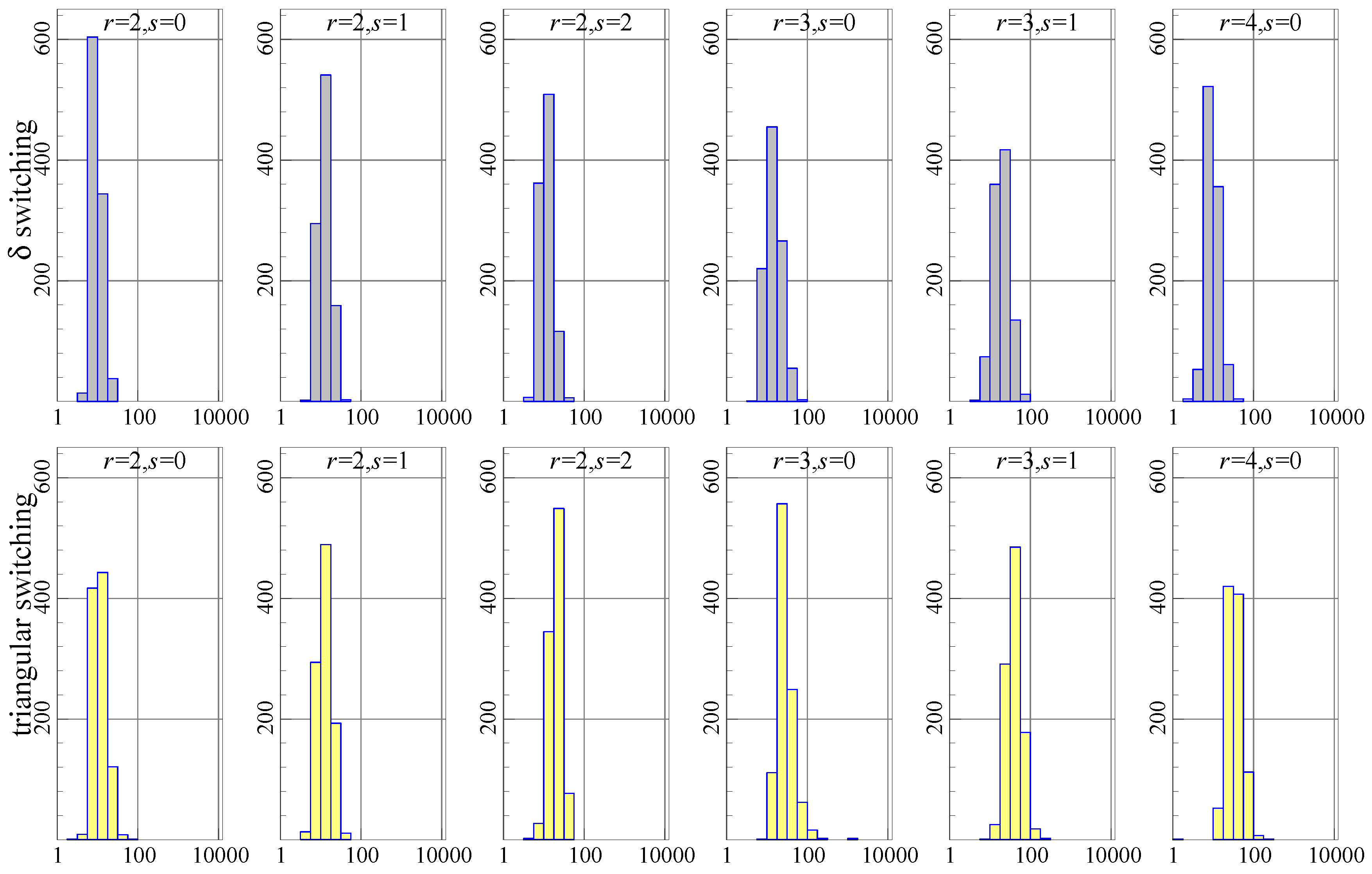
Figure 1 shows the histograms of the number of iterations required to achieve convergence (or 10,000). Each graph has the number of iterations (on a log 10 scale) on the horizontal axis and the count (out of 1000 experiments) represented by the bars and the vertical axis. Ideally, all of the mass is to the left, reflecting very quick convergence. The top row of histograms is for $\delta$ switching, the bottom row for triangular switching. In each histogram, the data generation process (DGP) uses the stated $r,s$ values, and estimation is using the correct values of $r,s$.

The histograms show that triangular switching (bottom row) uses more iterations than $\delta$ switching (top row), in particular when $s=0$. Nonetheless, the experiment using triangular switching runs slightly faster as measured by the total time taken (and $\tau$ switching is the slowest).

An important question is whether the algorithms converge to the same maximum. The function value that is maximized is:

$$f\left(\theta \right)=-log|\Omega (\theta \left)\right|.$$

Out of 10,000 experiments, counted over all $r,s$ combinations that we consider, there is only a single experiment with a noticeable difference in $f(\widehat{\theta })$. This happens for $r=3,s=0$, and $\delta$-switching finds a higher function value by almost $0.05$. Because $T=119$, the $0.05$ translates to a difference of three in the log-likelihoods.

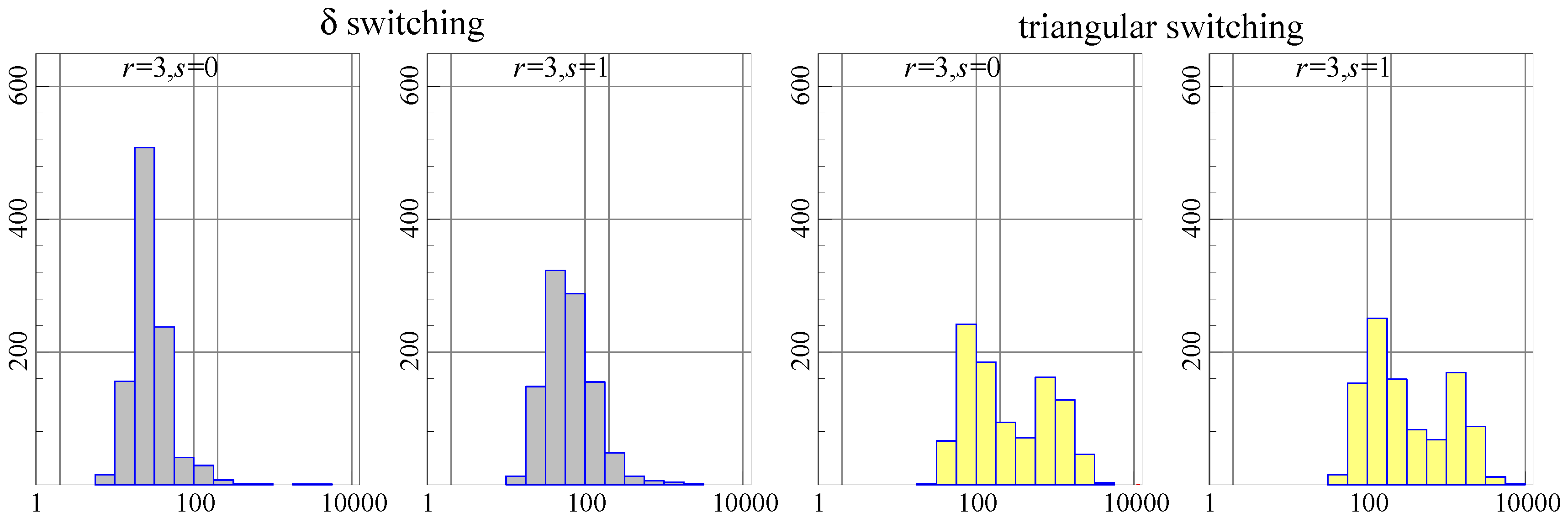
A second issue of interest is how the algorithms perform when restrictions are imposed. The following restrictions are imposed on the three columns of $\beta$ with $r=3$:

$$\begin{array}{ccccccc}& \hfill m_3& \hfill y& \hfill \Delta p& \hfill r_m& \hfill r_b& \hfill t\\ {\beta }_1^{\prime }\hfill & \hfill a& \hfill -a& \hfill 0& \hfill 1& \hfill -1& \hfill \ast \\ {\beta }_2^{\prime }\hfill & \hfill 0& \hfill \ast & \hfill 1& \hfill -a& \hfill a& \hfill \ast \\ {\beta }_3^{\prime }\hfill & \hfill 0& \hfill 0& \hfill 1& \hfill \ast & \hfill 0& \hfill \ast \end{array}$$

This specification identifies the cointegrating vectors and imposes two over-identifying restrictions. For $r=3,s=0$ this is accepted with a p-value of $0.4$, while for $r=3,s=1$, the p-value is $0.5$ using the model on the actual Danish data. Simulation is from the estimated restricted model.

In terms of the number of iterations, as Figure 2 shows, $\delta$-switching converges more rapidly in most cases. This makes triangular switching slower, but only by about $10\%$–$20\%$.

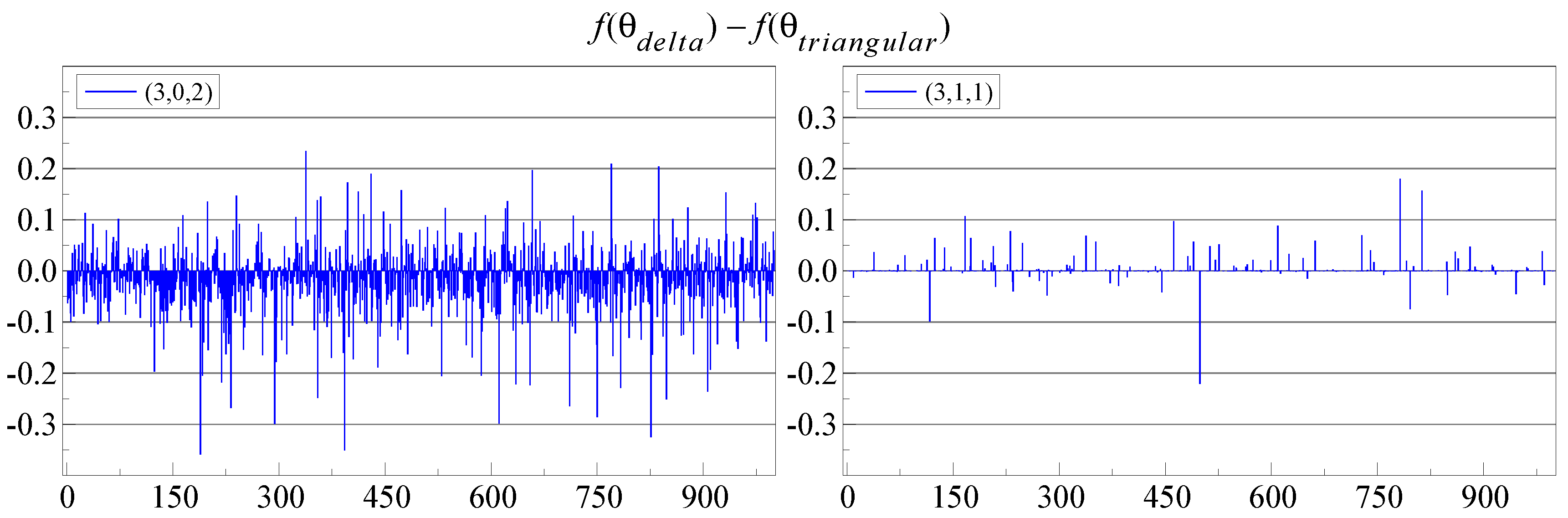
Figure 3 shows $f({\widehat{\theta }}_{\delta })-f({\widehat{\theta }}_{\mathrm{triangular}})$, so a positive value means that triangular switching obtained a lower log-likelihood. There are many small differences, mostly to the advantage of $\delta$-switching when $s=1$ (right-hand plot), but to the advantage of triangular switching on the left, when $s=0$. The latter case is also much more noisy.

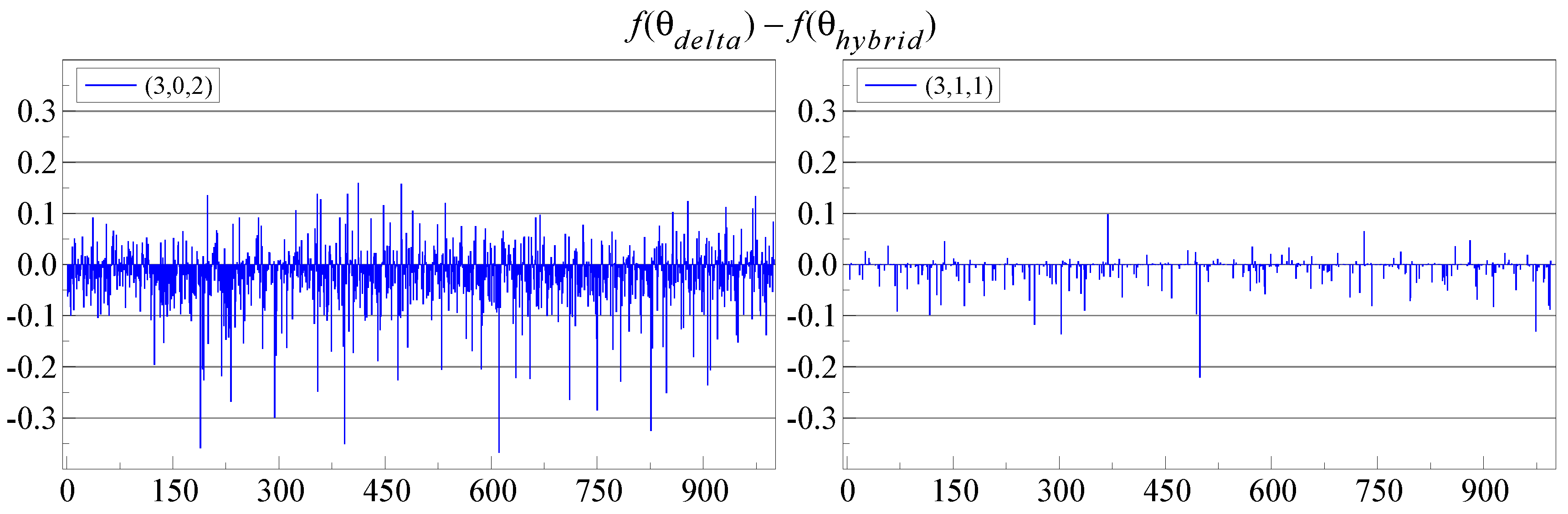
6.1. Hybrid Estimation

To increase the robustness of the triangular procedure, we also consider a hybrid procedure, which combines algorithms as follows:

• standard starting values, as well as twenty randomized starting values, then
• triangular switching, followed by
• BFGS optimization (the Broyden-Fletcher, Goldfarb, and Shanno quasi-Newton method) for a maximum of 200 iterations, followed by
• triangular switching.

This offers some protection against false convergence, because BFGS is based on first derivatives combined with an approximation to the inverse Hessian.

More importantly, we add a randomized search for better starting values as perturbations of the default starting values. Twenty versions of starting values are created this way, and each is followed for ten iterations. Then, we discard half, merge (almost) identical ones and run another ten iterations. This is repeated until a single one is left.

Figure 4 shows that this hybrid approach is an improvement: now, it is almost never beaten by $\delta$ switching. Of course, the hybrid approach is a bit slower again. The starting value procedure for $\delta$ switching could be improved in the same way.

7. Conclusions

We introduced the triangular representation of the I(2) model and showed how it can be used for estimation. The trilinear form of the triangular representation has the advantage that estimation can be implemented as alternating least squares, without using reduced-rank regression. This structure allows us to impose restrictions on (parts of) the A and B matrices, which gives more flexibility than is available in the $\delta$ and $\tau$ representations.

We also presented an algorithm based on the $\delta$-representation and compared the performance to triangular switching in an application based on Danish data, as well as a parametric bootstrap using that data. Combined with the acceleration of Doornik (2017), both algorithms are fast and give mostly the same result. This will improve empirical applications of the I(2) model and facilitate recursive estimation and Monte Carlo analysis. Expressions for the computation of t-values of coefficients will be reported in a separate paper.

Because they are considerably faster than the previous generation, bootstrapping the I(2) model can now be considered, as Cavaliere et al. (2012) did for the I(1) model.

References

- Anderson, Theodore W. 1951. Estimating linear restrictions on regression coefficients for multivariate normal distributions. Annals of Mathematical Statistics 22: 327–51, (Erratum in Annals of Statistics 8, 1980). [Google Scholar] [CrossRef]
- Anderson, Theodore W. 2002. Reduced rank regression in cointegrated models. Journal of Econometrics 106: 203–16. [Google Scholar] [CrossRef]
- Boswijk, H. Peter. 2010. Mixed Normal Inference on Multicointegration. Econometric Theory 26: 1565–76. [Google Scholar] [CrossRef]
- Boswijk, H. Peter, and Jurgen A. Doornik. 2004. Identifying, Estimating and Testing Restricted Cointegrated Systems: An Overview. Statistica Neerlandica 58: 440–65. [Google Scholar] [CrossRef]
- Cavaliere, Giuseppe, Anders Rahbek, and R.A.M. Taylor. 2012. Bootstrap Determination of the Co-Integration Rank in Vector Autoregressive Models. Econometrica 80: 1721–40. [Google Scholar]
- Dennis, Jonathan G., and Katarina Juselius. 2004. CATS in RATS: Cointegration Analysis of Time Series Version 2. Technical Report. Evanston: Estima. [Google Scholar]
- Doornik, Jurgen A. 2013. Object-Oriented Matrix Programming using Ox, 7th ed. London: Timberlake Consultants Press. [Google Scholar]
- Doornik, Jurgen A. 2017. Accelerated Estimation of Switching Algorithms: The Cointegrated VAR Model and Other Applications. Oxford: Department of Economics, University of Oxford. [Google Scholar]
- Doornik, Jurgen A., and R. J. O’Brien. 2002. Numerically Stable Cointegration Analysis. Computational Statistics & Data Analysis 41: 185–93. [Google Scholar] [CrossRef]
- Golub, Gen H., and Charles F. Van Loan. 2013. Matrix Computations, 4th ed. Baltimore: The Johns Hopkins University Press. [Google Scholar]
- Johansen, Søren. 1988. Statistical Analysis of Cointegration Vectors. Journal of Economic Dynamics and Control 12: 231–54, Reprinted in R. F. Engle, and C. W. J. Granger, eds. 1991. Long-Run Economic Relationships. Oxford: Oxford University Press, pp. 131–52. [Google Scholar] [CrossRef]
- Johansen, Søren. 1991. Estimation and Hypothesis Testing of Cointegration Vectors in Gaussian Vector Autoregressive Models. Econometrica 59: 1551–80. [Google Scholar] [CrossRef]
- Johansen, Søren. 1992. A Representation of Vector Autoregressive Processes Integrated of Order 2. Econometric Theory 8: 188–202. [Google Scholar] [CrossRef]
- Johansen, Søren. 1995a. Likelihood-based Inference in Cointegrated Vector Autoregressive Models. Oxford: Oxford University Press. [Google Scholar]
- Johansen, Søren. 1995b. Identifying Restrictions of Linear Equations with Applications to Simultaneous Equations and Cointegration. Journal of Econometrics 69: 111–32. [Google Scholar] [CrossRef]
- Johansen, Søren. 1995c. A Statistical Analysis of Cointegration for I(2) Variables. Econometric Theory 11: 25–59. [Google Scholar] [CrossRef]
- Johansen, Søren. 1997. Likelihood Analysis of the I(2) Model. Scandinavian Journal of Statistics 24: 433–62. [Google Scholar] [CrossRef]
- Johansen, Søren, and Katarina Juselius. 1990. Maximum Likelihood Estimation and Inference on Cointegration—With Application to the Demand for Money. Oxford Bulletin of Economics and Statistics 52: 169–210. [Google Scholar] [CrossRef]
- Johansen, Søren, and Katarina Juselius. 1992. Testing Structural Hypotheses in a Multivariate Cointegration Analysis of the PPP and the UIP for UK. Journal of Econometrics 53: 211–44. [Google Scholar] [CrossRef]
- Johansen, Søren, and Katarina Juselius. 1994. Identification of the Long-run and the Short-run Structure. An Application to the ISLM Model. Journal of Econometrics 63: 7–36. [Google Scholar] [CrossRef]
- Juselius, Katarina. 2006. The Cointegrated VAR Model: Methodology and Applications. Oxford: Oxford University Press. [Google Scholar]
- Paruolo, Paolo. 2000a. Asymptotic Efficiency of the Two Stage Estimator in I(2) Systems. Econometric Theory 16: 524–50. [Google Scholar] [CrossRef]
- Paruolo, Paolo. 2000b. On likelihood-maximizing algorithms for I(2) VAR models. Mimeo. Varese: Universitá dell’Insubria. [Google Scholar]
- Paruolo, Paolo, and Anders Rahbek. 1999. Weak exogeneity in I(2) VAR Systems. Journal of Econometrics 93: 281–308. [Google Scholar] [CrossRef]
Figure 1.
Comparison of algorithms: -switching (top row) and triangular-switching (bottom row). Simulating a range of . Number of iterations on the horizontal axis, count (out of 1000) on the vertical.
Figure 2.
Comparison of algorithms: -switching (left two) and triangular-switching (right two). Simulating a range of . Number of iterations on the horizontal axis, count (out of 1000) on the vertical.
Figure 3.
-switching function value minus the triangular switching function value (vertical axis) for each replication (horizontal axis). Both starting from their default starting values. The labels are the cointegration indices .
Figure 4.
-switching function value minus the hybrid triangular-switching function value (vertical axis) for each replication (horizontal axis).