
Dependence between Stock Returns of Italian Banks and the Sovereign Risk


1
Dipartimento di Scienze dell’Economia, Università del Salento, 73100 Lecce, Italy
2
Faculty of Economics and Management, Free University of Bozen-Bolzano, 39100 Bozen-Bolzano, Italy
*
Author to whom correspondence should be addressed.
Econometrics 2017, 5(2), 23; https://doi.org/10.3390/econometrics5020023
Submission received: 16 March 2017
/
Revised: 1 June 2017
/
Accepted: 5 June 2017
/
Published: 8 June 2017
(This article belongs to the Special Issue Recent Developments in Copula Models)
Abstract
:We analyze the interdependence between the government yield spread and stock returns of the banking sector in Italy during the years 2003–2015. In a first step, we find that the Spearman’s rank correlation between the yield spread and the Italian banking system changed significantly after September 2008. According to this finding, we split the time window in two sub-periods. While we show that the dependence between the banking industry and changes in the yield spread increased significantly in the second time interval, we find no contagion effects from changes in the yield spread to returns of the banking system.
JEL Classification:
C14; C58; C631. Introduction
During the recent financial crisis, a strong nexus between the financial sector and the sovereign credit risk has emerged worldwide. This potentially dangerous linkage is particularly pronounced in Europe, where banks—compared to the US or UK—are more important for providing liquidity to the economy and hold a much higher share of local government debt. The home bias is extreme for countries in the periphery, where in 2011 the holdings of sovereign bonds amounted to more than 15% of GDP (Merler and Pisan-Ferry 2011). While the vicious spiral in Ireland started with problems in the financial sector and the bailouts triggered the sovereign default risk, the country’s high debt-to-GDP ratio seems to be the starting point of the problems for Italian banks (Acharya et al. 2012).
The distinct and peculiar Italian circumstances require an accurate analysis of the linkage between the sovereign risk and the banking sector. First, in the past, Italian banks were much more focused on classical business and were less exposed to risky financial products. Therefore, before 2008 they had lower Credit default swap (shortly, CDS) spreads than banks from other European countries (Acharya et al. 2012). Second, the amount of wealth invested by Italian banks in government bonds of their own country (the so-called home bias) is historically higher than in any other troubled country (Merler and Pisan-Ferry 2011). Moreover, Italian banks used part of the cheap liquidity offered by the European Central Bank (ECB) via the two long-term refinancing operations (LTROs) to further increase their exposure in government bonds to more than 40% until May 2012 (Bank of Italy 2012). Therefore, their fate is particularly linked to the creditworthiness of the state. In fact, rising credit spreads cause direct losses in the treasury of the banks Angeloni and Wolff 2012; De Bruyckere et al. 2013, and they have an impact (although less evidently) on the net interest income (Albertazzi et al. 2014). Furthermore, an increase in the government yield induces higher interest rates on loans and a consequent decline in the lending volume of banks. In addition and more generally, higher sovereign credit spreads might be a signal that potential future bailouts become less affordable.
Since the beginning of the European government crisis in the years from 2011 to 2013, the main issue has been how to mitigate the systemic risk and how to ensure that the future probability of such a crisis reoccurring is reduced. In particular, the relationship between sovereigns and the banking industry is still at the center of academic attention, and various papers have investigated different aspects of this issue (e.g., Baglioni and Cherubini (2013); Delis and Mylonidis (2011); Kalbaska and Gatkowski (2012); Kohonen (2014); Reboredo and Ugolinia (2015a, 2015b); Xu et al. (2017)). The current paper addresses the following three research questions: (1) Is there a statistically significant dependence between the sovereign default risk and the stock returns of Italian banks, especially in the period 2011–2013? (2) Do large and small capitalized banks differ with respect to this relationship? (3) Is an increasing sovereign risk transferred through contagion to the equity returns of Italian banks? Compared to the literature, as a methodological contribution our investigation is mainly based on a two-step approach. First, we remove possible heteroscedasticity in the estimation of the time-varying dependence by using a parametric filtering procedure. Second, the research questions are answered by referring to the framework of (rank-invariant) association measures and tail dependence (Patton 2012).
The remainder of the paper is organized as follows: Section 2 provides a discussion on the meaning of the idiom financial contagion and an overview of the tools for investigating the interdependence between the government yield spread and stock returns of the banking sector in Italy during the years 2003–2015. Section 3 provides a detailed description of our empirical analysis. Section 4 concludes and provides a discussion on the financial and policy implications of the empirical findings.
2. What Financial Contagion Is, and How to Detect It
Financial contagion refers to the diffusion of financial distress from one market/economy to another. In a recent survey by Pericoli and Sbracia (2003), for instance, various definitions of contagion are discussed that reflect the wide variety of meanings ascribed to this term. A contagious episode typically results in an unprecedented high correlation level among the affected systems: If a financial crisis arises, stock returns may start behaving more similarly than they did in the pre-crisis period. A common approach to detecting the occurrence of contagion therefore consists of identifying breaks in the transmission of shocks and inferring from them a significant rise in the correlation of asset returns. In practice, analysts compare cross-market correlations in tranquil and crisis periods, under the assumption that a significant rise in the correlation is caused by a break in the data-generating process. Such a method is consistent with the “very restrictive” definition of contagion provided by the World Bank (World Bank 2016).
Although increased correlation may provide one way of measurement, simultaneous jumps in correlation are hardly contagion per se. For instance, Pericoli and Sbracia (2003) define contagion as an episode with excessive comovements in prices and quantities, conditional upon a crisis occurring in one market or a group of markets, which cannot be explained by simple interdependence. A similar definition is provided by Kaminsky et al. (2003), who make an explicit condition, writing “Only if there is excess comovement in financial and economic variables [...] in response to a common shock do we consider it contagion”.
This paper contributes to the discussion in the following way. First, our technique avoids a potential sample selection bias (and consequently, spurious results) in the identification of specific shocks or tranquil/crisis periods. As Pericoli and Sbracia (2003) point out, the correct identification of the origin of the crisis matters—in particular for those tools based on correlation breakdown (i.e., structural breaks in correlation): Empirical analysis may be affected by a sample selection bias problem, which occurs whenever tests are conducted on ad hoc subsamples. Second, we refer to the “No Contagion, Only Interdependence” principle (see Forbes and Rigobon (2002)), since during turmoils some increase in comovements is merely an implication of interdependence. To be consistent with the previously mentioned definitions of contagion, we focus on the observed joint distribution function of the asset returns over the whole period, and we distinguish between comovements merely implied by interdependence, mainly related to the central region of the joint distribution, and comovements implied by contagious episodes, associated with the Left tail of the distribution (where extreme losses are located). We thus ground our analysis on the following general definition of financial contagion.
Definition 1.
Financial contagion stands for a significant increase in excessive comovements of prices above typical comovements.
Definition 1 first recalls the use of excessive comovements, and second, it implicitly requires a comparison between comovements associated with different regions of the whole joint distribution function. This definition is consistent with that provided in Bradley and Taqqu (2004, 2005), who locally analyze the dependence structure of the involved financial time series by using a linear measure of association. Definition 1 is also consistent with the group of empirical works on the international transmission of shocks, where contagion is defined in terms of discontinuities in the data-generating process, and its presence is tested by checking for structural breaks in correlation (see the classification in Pericoli and Sbracia (2003) and the references therein).
According to Definition 1, the key point is the specification of an appropriate measure of contagion, able to distinguish contagious episodes from simple interdependence. To illustrate our methodology, we exploit some results from early works (see Durante and Jaworski (2010); Durante and Foscolo (2013); Durante et al. (2013)), in which contagion in European markets during the Great Recession and the European sovereign debt crisis has been investigated.
Generally speaking, we say that there is contagion between market/asset X and market/asset Y if there is more dependence between X and Y when they perform (very) badly than when they exhibit a typical performance. Thus, contagion is related to the strength of the dependence between X and Y at different regions of the domain of the joint distribution of . Durante and Jaworski (2010) propose a contagion test grounded on the concept of copula (i.e., a function able to capture the rank-invariant dependency among random variables). Such an approach is based on the determination of a suitable threshold (i.e., quantile level) that draws a distinction between normal comovements due to simple interdependence and excessive comovements.
Let X and Y be the random variables representing the returns of two financial markets/assets. In order to analyze contagion according to our definition, we are interested in the conditional distribution function of , which is supposed to be well defined in the following, where the conditioning set is one of the following types:
- B is a tail set (usually denoted by T) that includes the realizations of that are judged to represent a risky scenario;
- B is a central set, or mediocre set (usually denoted by M) that includes the realizations of that are judged to represent an “untroubled scenario”.
In particular, we assume here that the tail and the central set can be defined as suitable rectangles of whose boundaries are determined by quantile levels of X and/or Y. For instance, given two financial markets X and Y, if the contagion from X to Y is of main interest, then the following sets can be considered:
- , representing possible extreme negative returns of X;
- , representing returns of X that are judged to be usual fluctuations in the markets.
Here, and is the quantile function associated with X.
As shown in Durante and Jaworski (2010), contagion can be introduced in terms of a suitable comparison between copulas associated with the joint conditional distribution of a tail and a central set (see Cherubini et al. (2011); Durante and Sempi (2016); Mai and Scherer (2012)). To this end, we recall here the definition of concordance ordering in the bivariate case; see Durante and Sempi (2016). Given two continuous random pairs and with marginal distribution functions and copulas and , respectively, is said to be more concordant than , written , if for all , and , . In order to indicate the case when but for at least one , the symbol ≺ is used.
Definition 2.
Let X and Y be the random variables representing the returns of two financial markets/assets. Let and be a tail and a central set, respectively, for which are determined by a suitable level α. Contagion between X and Y at the level exists if , where (respectively, ) is the copula of the conditional distribution function of (respectively, ).
Definition 2 has the following interesting features. It is a distribution-based notion, since it is grounded on the comparison between the dependence in a tail region (the copula related to the tail set) and the dependence in a central region (the copula of the central set) of the joint distribution function of . It is more informative than other methods based on linear Pearson’s correlation coefficient or tail dependence coefficients, since it is able to catch nonlinear dynamics and it is not restricted to the extreme tail. It depends on a suitable definition of tail (and central) set, according to the threshold . Finally, it appears when there is a strict order between the copulas. For instance, two markets that are perfectly comonotone (i.e., one market is an increasing function of the other) exhibit no (symmetric) contagion, since their dependence does not change at any time—these markets are simply interdependent.
Checking contagion as in Definition 2 could be difficult to implement in practice because the identification of the copula of the conditional distribution function of may be complicated. In order to avoid such troubles, a non-parametric procedure has been suggested by Durante and Jaworski (2010). Given two copulas C and D, if , then , where is the Spearman’s rank correlation coefficient (see Schmid et al. (2010), which for any pair of continuous random variables X and Y with copula C is given by
Then, we check the absence of contagion by comparing the values of the associated Spearman’s rank-correlation coefficient. The following test can be thus performed:
where and are the copulas associated with the conditional distribution function of X and Y with respect to the tail and the central set, respectively. We define , and its empirical counterpart. Under some mild assumptions on the involved threshold copulas (Durante and Jaworski 2010), the asymptotic behavior of is given by
where N stands for the sample size and the subscript of the variance term reflects the fact that the variance depends on the way the tail and the central sets are defined. By using the Gaussian approximation in Equation (1), a contagion test could be easily implemented. The one-sided hypothesis test procedure reads as follows (Dobric et al. 2013; Durante and Jaworski 2010):
- Compute and from the observations in and , for a given .
- Compute bootstrap replications from the entire sample.1 For each replication, calculate and , as well as the corresponding difference .
- On the basis of the vector of the bootstrap estimated difference between Spearman correlation coefficients , estimate the asymptotic variance of and calculate the test statistic , where is the bootstrap estimate of .
- Reject the null hypothesis if , where denotes the standard normal distribution function and the chosen significance level.
An approach connected with our methodology has been recently proposed by Li and Zhu (2014), who use Kendall’s tau instead of Spearman’s coefficient. There are two main differences between our procedure and that introduced in Li and Zhu (2014): First, our test statistic does not require the identification of the trigger events that discriminate tranquil and crisis periods, since it is implicitly determined by choosing a suitable threshold . Second, our methodology directly works on the dependence structure—it is grounded on the comparison between typical comovements, implied by interdependence and mainly related to the central region of the joint distribution, and excessive comovements implied by contagious episodes and associated with the tail of the joint distribution.
As shown by Durante et al. (2013), the occurrence of contagion strongly depends on the choice of the threshold —a fact that could represent a key point when one wants to draw conclusions from the empirical analysis.
A formal test of contagion may have the drawback that it cannot quantify the size of the “jump” in the comovement—information that could be useful for classifying different markets according to their “extreme” linkages. In order to provide this feature, an empirical measure of contagion has been proposed in Durante and Foscolo (2013), called Spearman’s Contagion Index (briefly, ). The at level is defined as
The domain of the is by construction : the higher the dependence in the tail of the distribution compared to its center, the larger the values of the (in absolute terms) as evidence of contagion. The assumes that during crisis times the correlation in the tail increases compared to the center. Under mild assumptions, the estimator of is asymptotically Gaussian distributed. Moreover, its variance—which depends on —can be estimated with bootstrapping, as explained in Durante and Jaworski (2010) and Dobric et al. (2013).
The value of may be interpreted as follows. If , then , which could indicate the presence of contagion. Analogously, if , then , and contagion does not occur. If there is no difference in the conditional correlation between tail and central set, then , meaning that no shift of the dependence structure has been realized. As for the test statistic, in order to prevent the arbitrary choice of , Durante et al. (2014) suggest an average measure of contagion, where the index is evaluated on an interval of threshold values.
The contagion index thus goes beyond the use of linear correlation: it can be calculated via non-parametric methods, and it does not require the specification of crisis/tranquil periods a priori. As such, it avoids possible problems of mis-specifying the dependence structure.
3. Data, Empirical Investigation, and Results
Our empirical analysis is based on first differences (i.e., changes) in the 10-year bond yield spread between Italy (TRYDE10Y-FDS) and Germany (TRYDE10Y-FDS), and log-returns of the FTSE Italy All Share Bank Index (T8300-FTX) over the period 01/2003–07/2015 (Datastream mnemonics in parenthesis). We use first differences, as changes in the yield spread influence the market price of government bonds. To measure the impact of changes in the yield spread on Italian banks, we rely on equity returns because they seem to lead other market indicators (e.g., CDS rates) (Fung et al. 2008; Norden and Weber 2009). In order to alleviate non-synchronous trading hours in the past, we stick to a weekly frequency Cappiello et al. 2006). Furthermore, we also use all time series of those constituents of the banking index (date July 2015) listed since January 2003, which corresponds to the start of the index and the start of our investigation period.
Figure 1 shows the evolution of the Italian yield spread (as solid black line) and the 1-year rolling window Spearman’s rank correlation between differences in yields and log-returns of the banking index (solid gray line) with 95% confidence intervals (dotted gray lines).2 While before 2008 the independence assumption between changes in yield spread and stock returns of the bank index cannot be rejected (at 5% level) according to a nonparametric test of independence for multivariate time series proposed by Genest and Rémillard (2004), afterwards it turned out that the Spearman’s rank correlation was significant. Given that Figure 1 suggests two different regimes for the correlation over time, we conduct the nonparametric test for change-point detection based on the (multivariate) empirical distribution function proposed by Holmes et al. (2013) and implemented in R by Kojadinovic (2015). We find a change-point to be located approximately at the end of September 2008,3 the time when the investment bank Lehman Brothers filed for Chapter 11 bankruptcy protection. Indeed, the Spearman’s correlation in the two highlighted periods is statistically different: While until September 2008 the correlation between the two time series is with a 95% block bootstrap confidence interval of (indicating that the independence assumption cannot be rejected at the 5% significance level), afterwards the correlation declines to with the corresponding confidence interval , with a peak of and a corresponding confidence interval in the period 2011–2013. We observe that the negative dependence is statistically significant after 2008. In the following, for simplicity we refer to these two time intervals as first and second period, respectively. For each period, we carry out a dependence analysis by estimating several measures of association between changes in the yield spread and stock returns of the banking system.
In order to focus on the contagion effect, following Forbes and Rigobon (2002) it should be considered that heteroscedasticity in the univariate financial time series might induce a bias in the estimation of the dependence. Moreover, the calculation of copula-based measures (like Spearman’s correlation) usually benefits from considering data that are not serially dependent. For all these reasons, it is convenient to filter each time series in each sub-period with a univariate time series model for the conditional mean and the conditional variance, and hence apply our methodology to the residuals of the fitted models. As shown in Rémillard (2017), the limiting distribution of rank-based dependence measures computed with the residuals are the same as if the dependence measures were computed with the innovation (i.e., they are able to detect the (marginal-free) dependence among the time series). Specifically, in order to capture stylized facts in financial markets, we assume that each time series follows an ARMA-GJR-GARCH model Glosten et al. 1993), whose standardized residuals have a constant conditional t-distribution. The Bayesian information criterion (BIC) is used to select the model order. The estimated standardized residuals are given by
where stands the observation of the time series j at time t, is the vector of estimated parameters for the ARMA models, is the vector of estimated parameters for the GJR-GARCH models, and stands for past information of the time series. The goodness-of-fit of this model choice is checked by different diagnostic tests. The Box–Ljung and the ARCH test (at one and four lags) assess the absence of residual autocorrelation and heteroscedasticity at a significance level of 1%. Moreover, the Kolmogorov–Smirnov test confirms the t-distribution assumption for the residuals, and the Augmented Dickey–Fuller test does not show the presence of unit roots at a significance level of 1%.4
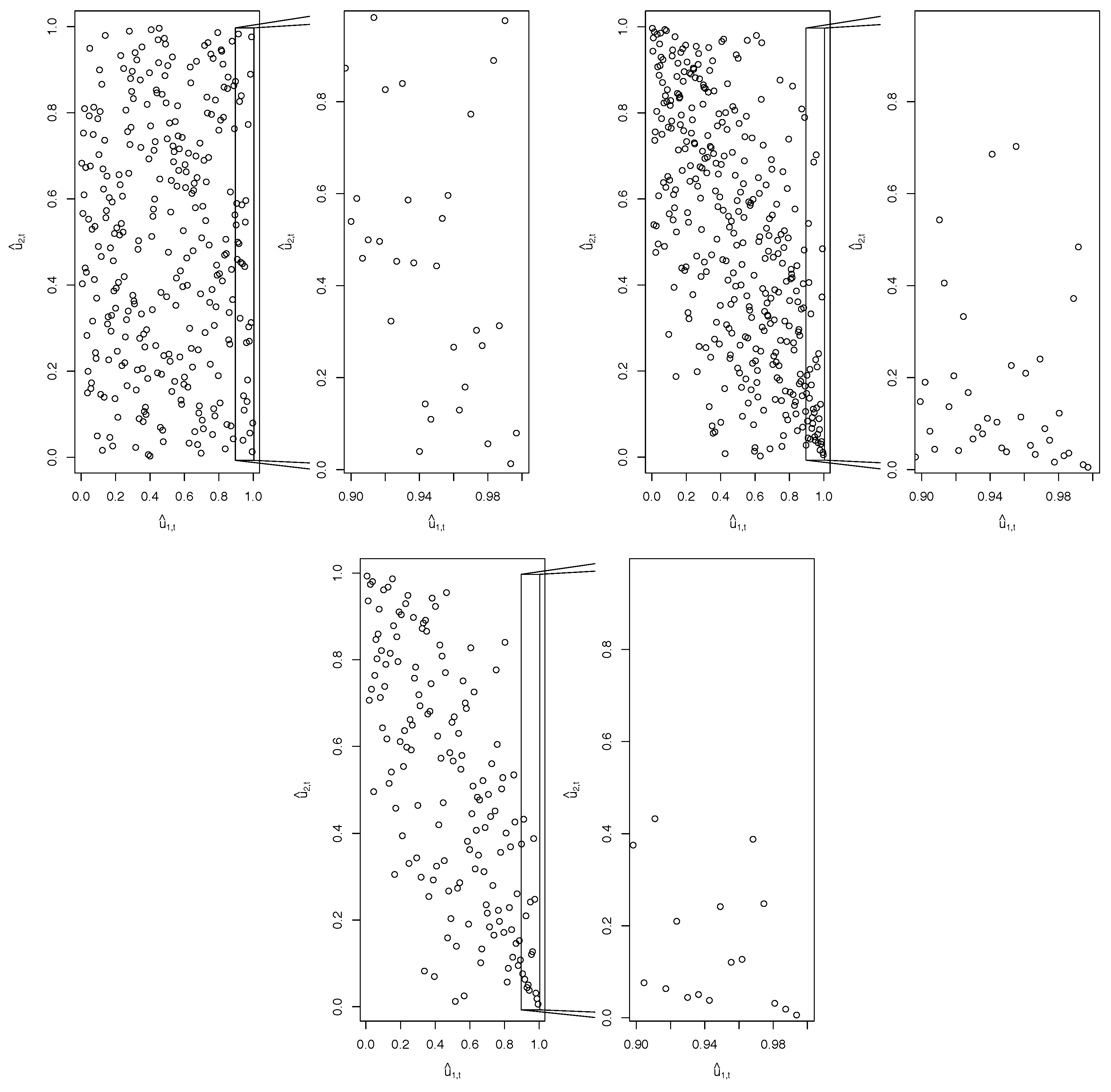
In order to focus on rank-invariant dependence, we further compute the so-called pseudo-observations : Therefore, for each time series and sub-period, the estimated standardized residuals have been sorted and scaled by ,5 where n stands for the sample size (Patton 2012). Figure 2 shows the scatter plot of pseudo-observations for the yield spread against the returns of the banking index , separately for the first (Upper Left Panel) and second period (Upper Right Panel), respectively, with a focus on the period 2011–2013 in the Bottom Panel of Figure 2. By focusing on the enlarged Right Rectangles of the bivariate distributions (which focus on the upper tail sets of the time series), for the second period we notice an increased (negative) dependence between high changes in the yield spread and low returns of the banking index, as previously quantified and shown in Figure 1; i.e., the Italian banking industry seems to suffer more under a severe increase in the sovereign default risk during the second period than during the first one.
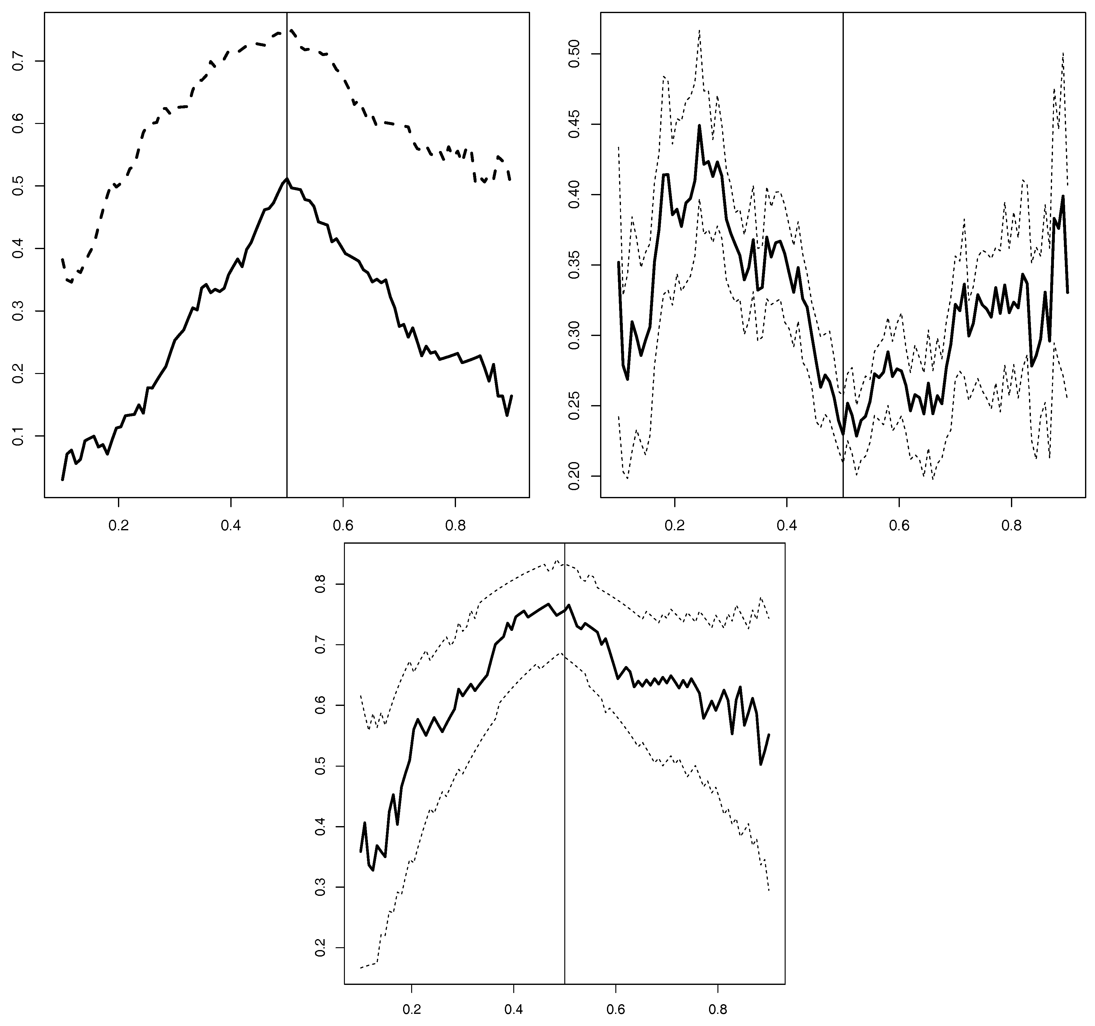
In order to analyze the behavior in the tails and to better understand the change observed in the second period, the Upper Left Panel of Figure 3 shows the estimated quantile dependence (also called tail concentration function, see Patton (2012) and Durante et al. (2015)) for the first period (solid line) and the second period (dashed line), respectively, by conditioning on the the yield spread. Once again, a focus on the period 2011–2013 is provided in the Bottom Panel of Figure 3. The upper quantile dependence is defined by
i.e., gives the probability to observe low pseudo-observations in stock returns conditional on high pseudo-observations in changes of the yield spread with ; analogously, the lower quantile dependence is defined by
with . Two findings are noteworthy. First, the right-tail quantile dependence is higher than the left-tail one in both periods. Therefore, the probability that large increases in the yield spread induce low stock returns is higher than for the contrary case of large declines in the yield spread. Second, the dependence in the second period (dashed line) is generally higher than in the first period (solid line). In the Upper Right Panel of Figure 3, we calculate the difference between the tail dependence in both periods together with 95% bootstrap confidence intervals. The figure confirms that for all quantile values the difference between the dependence in the two periods is statistically significant.
Finally, we use the Spearman’s contagion index proposed by Durante and Foscolo (2013) to quantify potential contagion effects from changes of the yield spread to returns of the banking index. The from to is defined by
where indicates the operator to calculate the Spearman correlation and the chosen quantile value. Figure 4 shows the for extreme pseudo-observations of changes in the yield spread by choosing with the 95% bootstrap confidence interval in the second period. Although the is negative, which indicates that the dependence in the tails is smaller than in the center, we cannot claim that our findings are statistically significant in the second period (as also confirmed by the formal test of contagion shown in Figure 7). Therefore, in line with other papers (Caporin et al. 2013; Forbes and Rigobon 2002; Serwa and Bohl 2005), we cannot claim that contagion effects caused the increased dependence in the recent past (compared to Broto and Perez-Quiros (2015); De Bruyckere et al. (2013)). We repeated the same exercise for other EU countries. Interestingly, the same conclusion—an unclear picture of contagion effects—applies to France (one core European country) and other peripheral countries (i.e., Greece, Ireland, Portugal, and Spain, respectively); see Figure 4.
3.1. Large vs. Small Banks
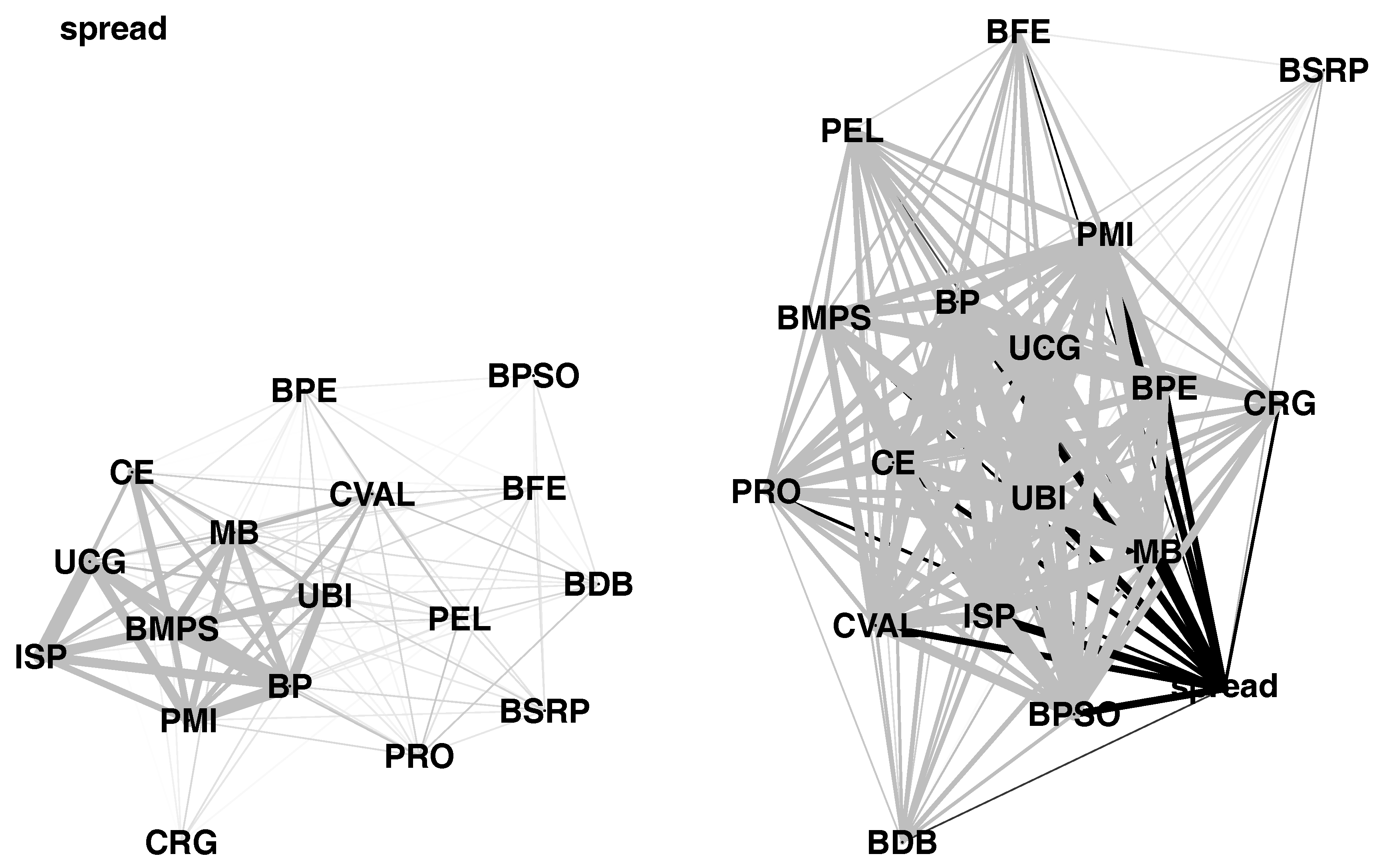
In Figure 5, we use a network representation to compare the dependence of pseudo-observations between changes in the yield spread and the returns of the single constituent Italian banks.6 The width of the lines shows the extent of the dependence, and the gray (respectively, black) color indicates a positive (respectively, negative) correlation.
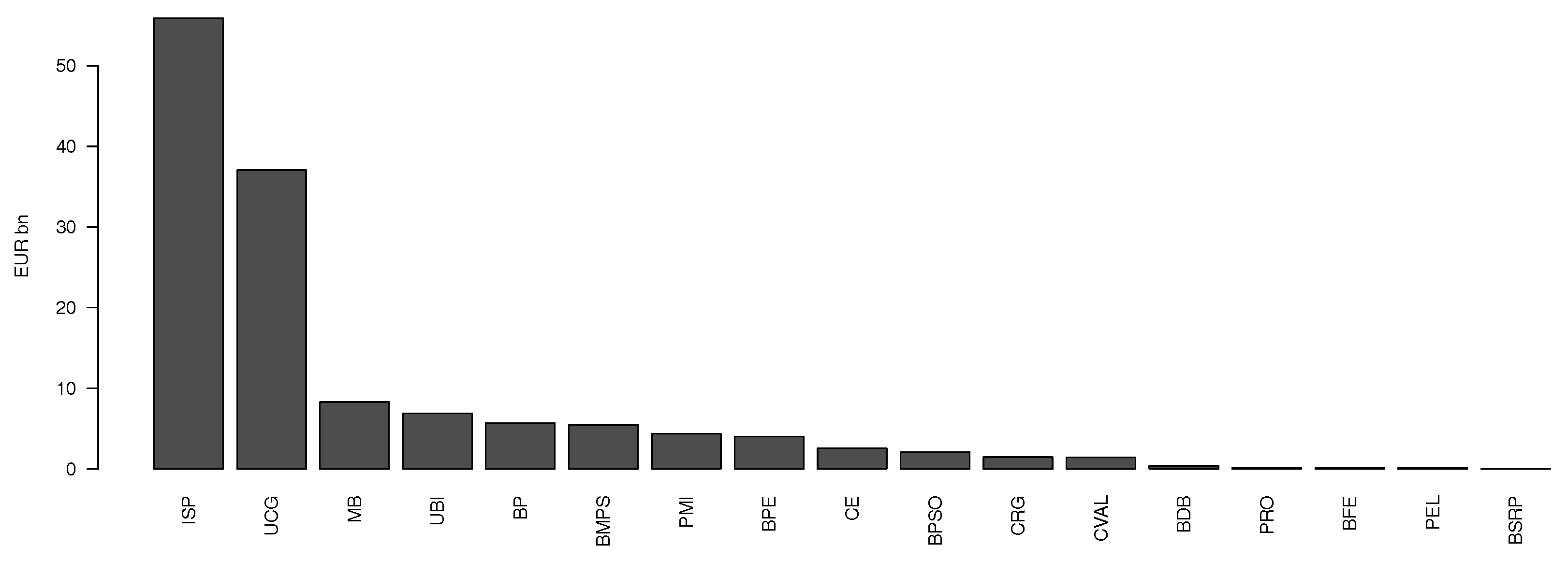
It can be easily seen that during the first period there is basically no relationship between changes in the yield spread and the single banks. During the second period, a high negative correlation (shown by thick black lines) between changes in the yield spread and the single banks can be observed. Furthermore, compared to the first period, the correlation among the banks seems to increase considerably. In order to investigate the relationship between the dependence and the size of the banks, in Figure 6 we indicate the corresponding market capitalization (in billions). By ranking the Italian banks according to their market capitalization, it can be seen that especially during the crisis period, large capitalized banks are highly and negatively correlated to changes in the yield spread (see the Right Panel of Figure 5). This might also explain the high correlation among the large capitalized banks at the center of the network, while small capitalized banks in the outer regions seem to be less affected.
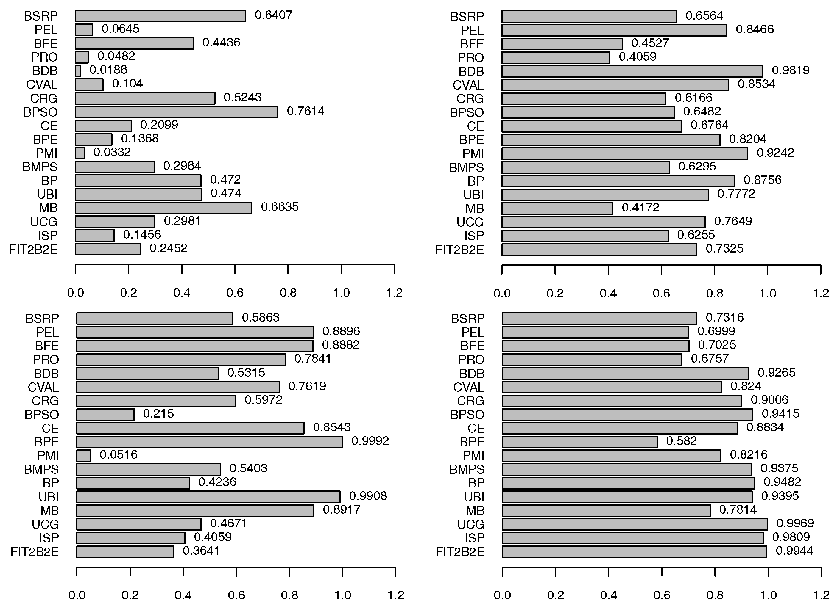
Despite the observed increased correlation in the second period, we are not able to detect a significant evidence of contagion from spread to banks in both periods (Figure 7, Upper Panels). Reverse causality has also been tested, since impaired interbank markets raised funding costs of all banks, and increased the expectations that governments have to bailout their indigenous banks. The contagion test procedure rejects this conjecture (Figure 7, Bottom Panels). Therefore, potential bi-directional contagious effects seem to be unlikely according to our methodology.
Figure 7.
p-values associated with the contagion test statistic at the level . In the (Upper Panels), the null hypothesis of absence of contagion from spread to banks is tested in the first (Left Panel) and second period (Right Panel), respectively. In the Bottom Panels, the null hypothesis of absence of contagion from banks to spread is tested in the first (Left Panel) and second period (Right Panel), respectively.

4. Conclusions
The two recent financial crises (the U.S. subprime mortgage crisis and the European Sovereign Debt Crisis) revealed significant deficiencies in both the analytical framework and the policymaker’s ability to mitigate emerging system-wide vulnerabilities. Macro-financial linkages have not been fully appreciated, and the transmission of risk across the financial systems has been severely underestimated. In the present paper, we propose a non-linear approach in order to measure the dependence between the sovereign credit spread and the stock returns of Italian banks. We find significant negative dependence starting from September 2008, but no contagion effects from the government yield spread to the banking system. As an interesting result, compared to small capitalized banks, during the second period large capitalized banks are highly and negatively correlated to changes in the yield spread. From the policymaker’s perspective, the proposed tools are useful in at least two ways: First, our method—which reduces the impact of arbitrary model choices—allows supervisors to monitor the banking system based on empirical evidence. Second, the insights of this exercise might be used to update necessary size-dependent capital buffers in response to an increased systematic risk in the market.
Acknowledgments
The authors are grateful to the referees for their valuable comments. A special thank to Ruggero Bertelli for his helpful suggestions on this paper. The second author acknowledges the support of Free University of Bozen-Bolzano via the projects “Handling High-Dimensional Systems in Economics” and “Financial Crisis Chronicles: Systemic Perspective and Econometric Issues (FINCH)”. The first and third author have been supported by Free University of Bozen-Bolzano via the project AIDA.
Author Contributions
All authors contributed equally to the paper.
Conflicts of Interest
The authors declare no conflict of interest.
References
- Acharya, Viral V., Itamar Drechsler, and Philipp Schnabl. 2012. A tale of two overhangs: The nexus of financial sector and sovereign credit risks. Banque de France—Financial Stability Review, 51–56. [Google Scholar]
- Albertazzia, Ugo, Tiziano Ropeleb, Gabriele Seneb, and Federico Maria Signorettib. 2014. The impact of the sovereign debt crisis on the activity of Italian banks. Journal of Banking & Finance 46: 387–402. [Google Scholar]
- Angeloni, Chiara, and Guntram B. Wolff. 2012. Are Banks Affected by Their Holdings of Government Debt? Technical Report, Bruegel Working Paper. Brussels: Bruegel. [Google Scholar]
- Baglioni, Angelo, and Umberto Cherubini. 2013. Within and between systemic country risk. Theory and evidence from the sovereign crisis in Europe. Journal of Economic Dynamics and Control 37: 1581–97. [Google Scholar] [CrossRef]
- Bank of Italy. 2012. Economic Bulletin. Available online: https://tinyurl.com/y6u4cb2u (accessed on 16 March 2017).
- Bradley, Brendan, and Murad S. Taqqu. 2004. Framework for analyzing spatial contagion between financial markets. Finance Letters 2: 8–15. [Google Scholar]
- Bradley, Brendan, and Murad S. Taqqu. 2005. Empirical evidence on spatial contagion between financial markets. Finance Letters 3: 77–86. [Google Scholar]
- Broto, Carmen, and Gabriel Perez-Quiros. 2015. Disentangling contagion among Sovereign CDS spreads during the European debt crisis. Journal of Empirical Finance 32: 165–79. [Google Scholar] [CrossRef]
- Caporin, Massimiliano, Loriana Pelizzon, Francesco Ravazzolo, and Roberto Rigobon. 2013. Measuring Sovereign Contagion in Europe. Technical Report. National Bureau of Economic Research. [Google Scholar] [CrossRef]
- Cappiello, Lorenzo, Robert F. Engle, and Kevin Sheppard. 2006. Asymmetric dynamics in the correlations of global equity and bond returns. Journal of Financial Econometrics 4: 537–72. [Google Scholar] [CrossRef]
- Cherubini, Umberto, Sabrina Mulinacci, Fabio Gobbi, and Silvia Romagnoli. 2011. Dynamic Copula Methods in Finance. New York: John Wiley & Sons. [Google Scholar]
- Davison, Anthony Christopher, and David Victor Hinkley. 1997. Bootstrap Methods and Their Application. Cambridge: Cambridge University Press. [Google Scholar]
- De Bruyckerea, Valerie, Maria Gerhardtb, Glenn Schepensc, and Rudi Vander Vennetb. 2013. Bank/sovereign risk spillovers in the European debt crisis. Journal of Banking & Finance 37: 4793–809. [Google Scholar]
- Delis, Manthos D., and Nikolaos Mylonidis. 2011. The chicken or the egg? A note on the dynamic interrelation between government bond spreads and credit default swaps. Finance Research Letters 8: 163–70. [Google Scholar] [CrossRef]
- Dobric, Jadran, Gabriel Frahm, and Friedrich Schmid. 2013. Dependence of stock returns in bull and bear markets. Depend Model 1: 94–110. [Google Scholar] [CrossRef]
- Durante, Fabrizio, and Piotr Jaworski. 2010. Spatial contagion between financial markets: A copula-based approach. Applied Stochastic Models in Business and Industry 26: 551–64. [Google Scholar] [CrossRef]
- Durante, Fabrizio, and Enrico Foscolo. 2013. An analysis of the dependence among financial markets by spatial contagion. International Journal of Intelligent Systems 28: 319–31. [Google Scholar] [CrossRef]
- Durante, Fabrizio, Enrico Foscolo, and Miroslav Sabo. 2013. A Spatial Contagion Test for Financial Markets. In Synergies of Soft Computing and Statistics for Intelligent Data Analysis. Edited by Rudolf Kruse, Michael R. Berthold, Christian Moewes, María Ángeles Gil, Przemysław Grzegorzewski and Olgierd Hryniewicz. Advances in Intelligent Systems and Computing. Berlin and Heidelberg: Springer, vol. 190, pp. 313–20. [Google Scholar]
- Durante, Fabrizio, Juan Fernández-Sánchez, and Roberta Pappadà. 2015. Copulas, diagonals and tail dependence. Fuzzy Sets and Systems 264: 22–41. [Google Scholar] [CrossRef]
- Durante, Fabrizio, Enrico Foscolo, Piotr Jaworski, and Hao Wang. 2014. A spatial contagion measure for financial time series. Expert Systems with Applications 41: 4023–34. [Google Scholar] [CrossRef]
- Durante, Fabrizio, and Carlo Sempi. 2016. Principles of Copula Theory. Boca Raton: CRC/Chapman & Hall. [Google Scholar]
- Forbes, Kristin J., and Roberto Rigobon. 2002. No contagion, only interdependence: Measuring stock market comovements. The Journal of Finance 57: 2223–61. [Google Scholar] [CrossRef]
- Fung, Hung-Gay, Gregory E. Sierra, Jot Yau, and Gaiyan Zhang. 2008. Are the U.S. stock market and credit default swap market related? Evidence from the CDX Indices. The Journal of Alternative Investments 11: 43–61. [Google Scholar] [CrossRef]
- Genest, Christian, and Bruno Rémillard. 2004. Tests of Independence and Randomness Based on the Empirical Copula Process. Test 13: 335–69. [Google Scholar] [CrossRef]
- Glosten, Lawrence R., Ravi Jagannathan, and David E. Runkle. 1993. On the Relation between the Expected Value and the Volatility of the Nominal Excess Return on Stocks. The Journal of Finance 48: 1779–801. [Google Scholar] [CrossRef]
- Holmes, Mark, Ivan Kojadinovic, and Jean-François Quessy. 2013. Nonparametric tests for change-point detection à la Gombay and Horváth. Journal of Multivariate Analysis 115: 16–32. [Google Scholar] [CrossRef]
- Kalbaska, Alesia, and Mateusz Gątkowski. 2012. Eurozone sovereign contagion: Evidence from the CDS market (2005–2010). Journal of Economic Behavior and Organization 83: 657–73. [Google Scholar] [CrossRef]
- Kaminsky, Graciela L., Carmen M. Reinhart, and Carlos A. Vegh. 2003. The Unholy Trinity of Financial Contagion. The Journal of Economic Perspectives 17: 51–74. [Google Scholar] [CrossRef]
- Kohonen, Anssi. 2014. Transmission of government default risk in the eurozone. Journal of International Money and Finance 47: 71–85. [Google Scholar] [CrossRef]
- Kojadinovic, Ivan. 2015. npcp: Some Nonparametric Tests for Change-Point Detection in Possibly Multivariate Observations, R package version 0.1-6; Available online: https://cran.r-project.org/package=npcp (accessed on 16 March 2017).
- Li, Fuchun, and Hui Zhu. 2014. Testing for financial contagion based on a nonparametric measure of the cross-market correlation. Review of Financial Economics 23: 141–47. [Google Scholar] [CrossRef]
- Mai, Jan-Frederik, and Matthias Scherer. 2012. Simulating Copulas: Stochastic Models, Sampling Algorithms, and Applications. Singapore: World Scientific. [Google Scholar]
- Merler, Silvia, and Jean Pisani-Ferry. 2011. Who’s afraid of sovereign bonds? Bruegel Policy Contribution 2012: 1–8. [Google Scholar]
- Norden, Lars, and Martin Weber. 2009. The co-movement of credit default swap, bond and stock markets: An empirical analysis. European Financial Management 15: 529–62. [Google Scholar] [CrossRef]
- Patton, Andrew J. 2012. A review of copula models for economic time series. Journal of Multivariate Analysis 110: 4–18. [Google Scholar] [CrossRef]
- Pericoli, Marcello, and Massimo Sbracia. 2003. A primer on financial contagion. Journal of Economic Surveys 17: 571–608. [Google Scholar] [CrossRef]
- Reboredo, Juan C., and Andrea Ugolini. 2015a. A vine-copula conditional value-at-risk approach to systemic sovereign debt risk for the financial sector. The North American Journal of Economics and Finance 32: 98–123. [Google Scholar] [CrossRef]
- Reboredo, Juan C., and Andrea Ugolini. 2015b. Systemic risk in European sovereign debt markets: A CoVaR-copula approach. Journal of International Money and Finance 51: 214–44. [Google Scholar] [CrossRef]
- Rémillard, Bruno. 2017. Goodness-of-fit tests for copulas of multivariate time series. Econometrics 5: 13. [Google Scholar] [CrossRef]
- Schmid, Friedrich, Rafael Schmidt, Thomas Blumentritt, Sandra Gaißer, and Martin Ruppert. 2010. Copula-based measures of multivariate association. In Copula Theory and Its Applications. Edited by Piotr Jaworski, Fabrizio Durante, Wolfgang Karl Härdle and Tomasz Rychlik. Lecture Notes in Statistics. Berlin: Springer, vol. 198, pp. 209–36. [Google Scholar]
- Serwa, Dobromił, and Martin T. Bohl. 2005. Financial contagion vulnerability and resistance: A comparison of European stock markets. Economic Systems 29: 344–62. [Google Scholar] [CrossRef]
- World Bank. 2016. Definitions of Contagion. Available online: https://tinyurl.com/pkrebnc (accessed on 16 March 2017).
- Xu, Simon, Francis In, Catherine Forbes, and Inchang Hwang. 2017. Systemic risk in the European sovereign and banking system. Quantitative Finance 17: 633–56. [Google Scholar] [CrossRef]
| 1 | The length of the simulated time series is typically set equal to the size of the original sample. |
| 2 | We calculate the confidence intervals by using the adjusted bootstrap percentile method Davison and Hinkley 1997). For the (linear) Pearson correlation (not shown) the graph is qualitatively similar. |
| 3 | 22 September 2008–26 September 2008. |
| 4 | All results of the different tests are available upon request. |
| 5 | This asymptotically negligible scaling factor is used to force the variates to fall inside the open unit hypercube. |
| 6 | The list of the Italian banks: Intesa Sanpaolo (ISP), Unicredit (UCG), Mediobanca (MB), Unione di Banche Italiane (UBI), Banco Popolare (BP), Monte dei Paschi di Siena (BMPS), Popolare di Milano (PMI), Popolare dell Emilia Romagna (BPE), Credito Emiliano (CE), Popolare di Sondrio (BPSO), Carige (CRG), Credito Valtellinese (CVAL), Desio e Brianza (BDB), Banca Profilo (PRO), Finnat Euramerica (BFE), Popolare Etruria Lazio (PEL), Banco di Sardegna (BSRP). |
Figure 1.
In the Upper Panel, the black solid line shows the evolution of the Italian yield spread. The solid gray line indicates the rolling 1-year Spearman’s rank correlation between FTSE Italy All Share Bank Index and the 10-year yield spread (the gray dotted lines give the 95% confidence interval); The Bottom Panel highlights the period 2011–2013.
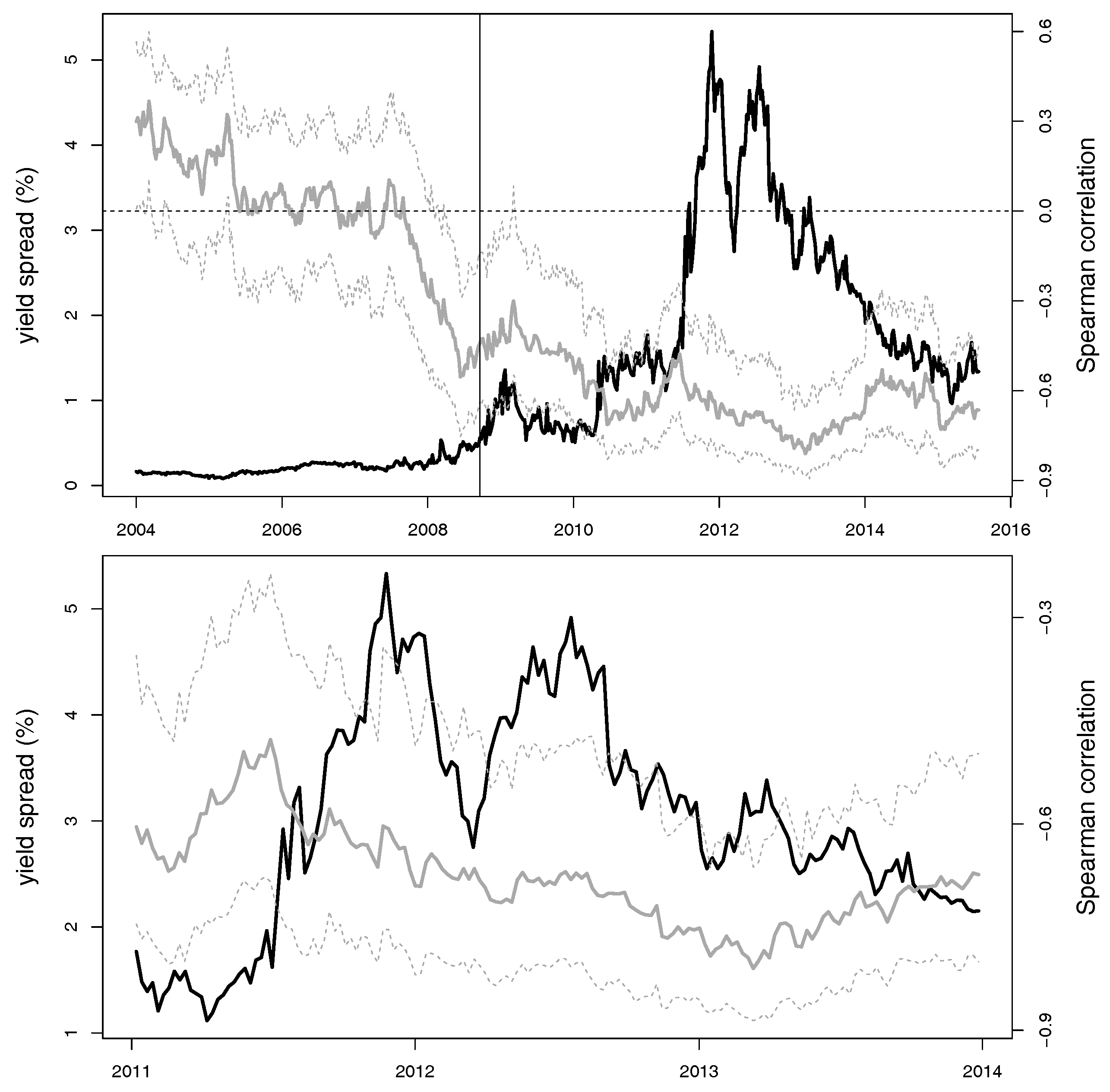
Figure 2.
Scatter plots of pseudo-observations between the yield spread and the FTSE All Share Banks index for the first (second) period are given in the Upper Left (Right) Panel. The scatter plot in the Bottom Panel focuses on the period 2011–2013.
Figure 2.
Scatter plots of pseudo-observations between the yield spread and the FTSE All Share Banks index for the first (second) period are given in the Upper Left (Right) Panel. The scatter plot in the Bottom Panel focuses on the period 2011–2013.

Figure 3.
The Upper Left Panel shows the estimated quantile dependence between the pseudo-observations of the yield spread and the FTSE All Share Banks index in the first (solid line) and second (dashed line) periods, while the Bottom Panel shows the estimated quantile dependence in the period 2011–2013 with a 95% bootstrap confidence interval. The Upper Right Panel presents the difference of the tail dependence estimates between the second and the first period along with a 95% bootstrap confidence interval.

Figure 4.
Spearman’s contagion index (overlay points) for extreme changes in the yield spread ( in descending order, respectively) during the second period for Italy, France, Greece, Ireland, Portugal, and Spain, respectively, along with the 95% bootstrap confidence interval (solid lines).
Figure 4.
Spearman’s contagion index (overlay points) for extreme changes in the yield spread ( in descending order, respectively) during the second period for Italy, France, Greece, Ireland, Portugal, and Spain, respectively, along with the 95% bootstrap confidence interval (solid lines).
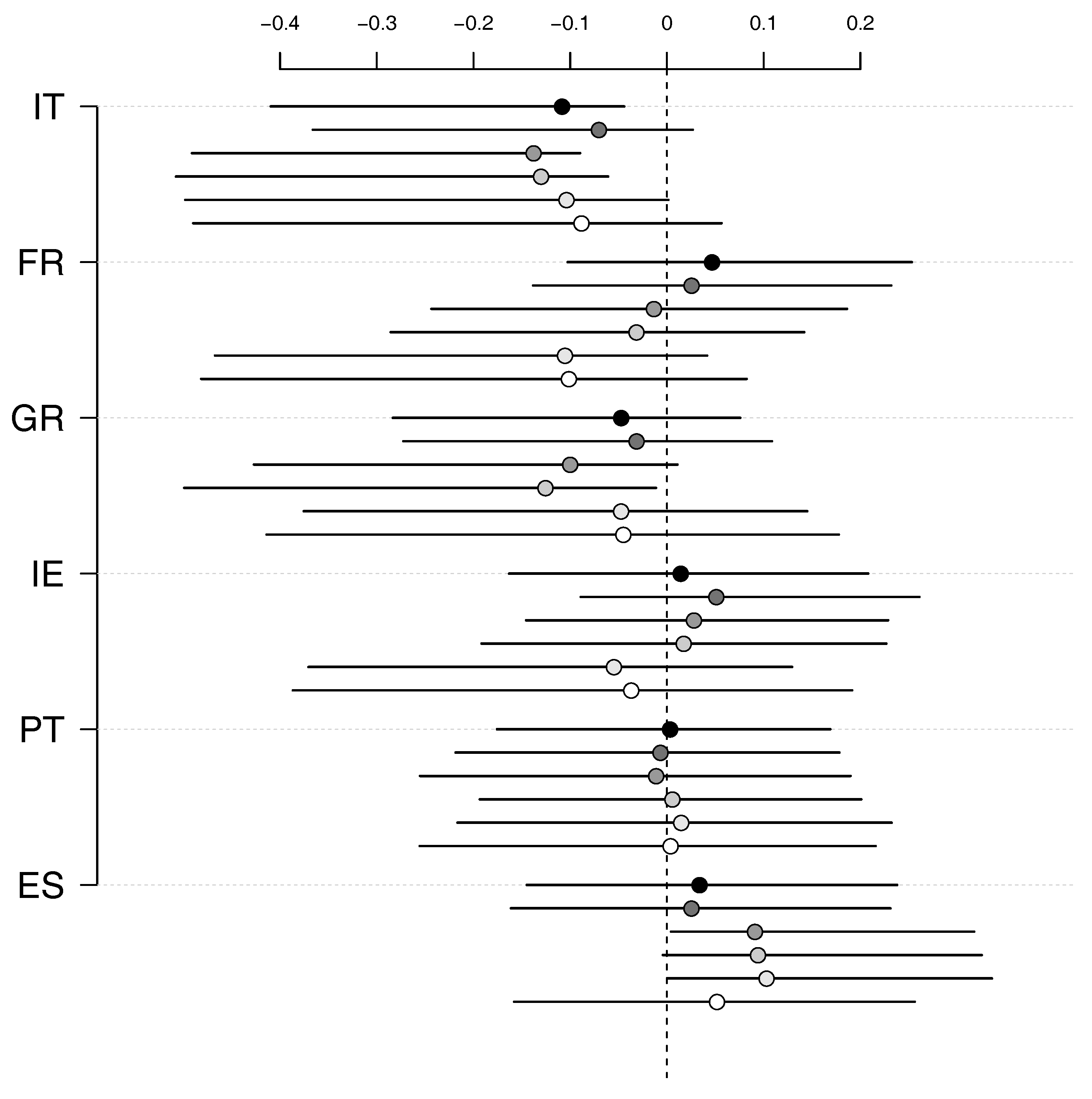
Figure 5.
Networks derived from the Spearman’s rank correlation between the pseudo-observations of changes in the yield spread and the equity returns of the single banks (first period on the Left and second period on the Right, respectively). The width of the lines shows the extent of the dependence, and gray (black) color indicates a positive (negative) correlation. BDB: Desio e Brianza; BFE: Finnat Euramerica; BMPS: Monte dei Paschi di Siena; BP: Banco Popolare; BPE: Popolare dell Emilia Romagna; BPSO: Popolare di Sondrio; BSRP: Banco di Sardegna; CE: Credito Emiliano; CRG: Carige; CVAL: Credito Valtellinese; ISP: Intesa Sanpaolo; MB: Mediobanca; PEL: Popolare Etruria Lazio; PMI: Popolare di Milano; PRO: Banca Profilo; UBI: Unione di Banche Italiane; UCG: Unicredit.

Figure 6.
Market capitalization of the single constituent banks.

© 2017 by the authors. Licensee MDPI, Basel, Switzerland. This article is an open access article distributed under the terms and conditions of the Creative Commons Attribution (CC BY) license (http://creativecommons.org/licenses/by/4.0/).
Share and Cite
MDPI and ACS Style
Durante, F.; Foscolo, E.; Weissensteiner, A. Dependence between Stock Returns of Italian Banks and the Sovereign Risk. Econometrics 2017, 5, 23. https://doi.org/10.3390/econometrics5020023
AMA Style
Durante F, Foscolo E, Weissensteiner A. Dependence between Stock Returns of Italian Banks and the Sovereign Risk. Econometrics. 2017; 5(2):23. https://doi.org/10.3390/econometrics5020023
Chicago/Turabian StyleDurante, Fabrizio, Enrico Foscolo, and Alex Weissensteiner. 2017. "Dependence between Stock Returns of Italian Banks and the Sovereign Risk" Econometrics 5, no. 2: 23. https://doi.org/10.3390/econometrics5020023
Note that from the first issue of 2016, this journal uses article numbers instead of page numbers. See further details here.