Using a Theory-Consistent CVAR Scenario to Test an Exchange Rate Model Based on Imperfect Knowledge

Abstract

A theory-consistent CVAR scenario describes a set of testable regularieties one should expect to see in the data if the basic assumptions of the theoretical model are empirically valid. Using this method, the paper demonstrates that all basic assumptions about the shock structure and steady-state behavior of an an imperfect knowledge based model for exchange rate determination can be formulated as testable hypotheses on common stochastic trends and cointegration. This model obtaines remarkable support for almost every testable hypothesis and is able to adequately account for the long persistent swings in the real exchange rate.

1. Introduction

International macroeconomics is known for its many pricing puzzles, including the purchasing power parity (PPP) puzzle, the exchange rate disconnect puzzle, and the forward rate puzzle. The basic problem stems from an inability of standard models based on the rational expectations hypothesis (REH) to account for highly persistent deviations from PPP and uncovered interest parity (UIP). See Engel (2014) and references therein for studies on REH and behavioral models.

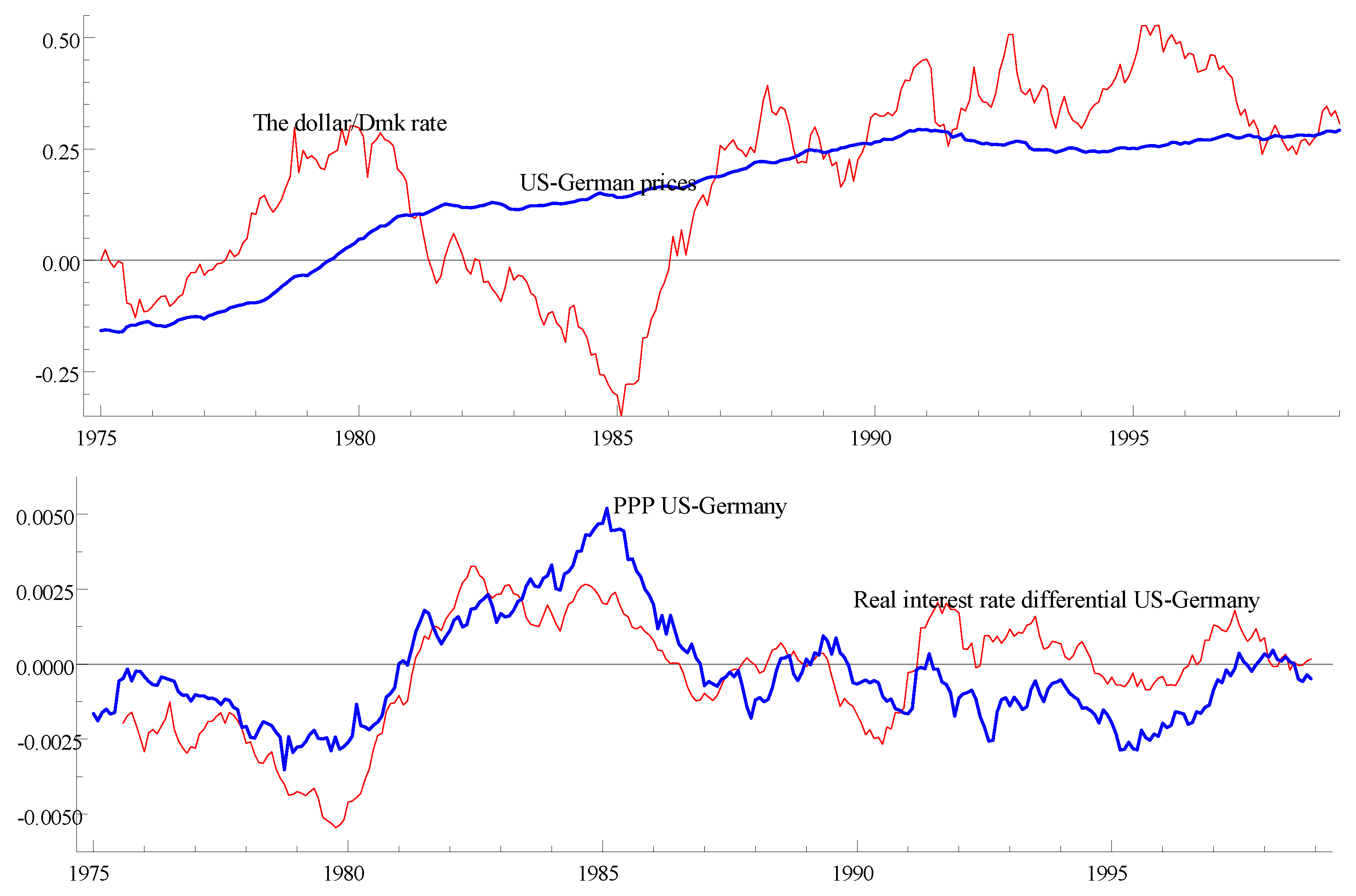
Figure 1 illustrates the long swings in the nominal and the real exchange rate that have puzzled economists for decades. The upper panel shows relative prices for the USA and Germany together with the nominal Deutshemark/Dollar rate for the post-Bretton Woods, pre-EMU period. While both series exhibit a similar upward sloping trend defining the long-run fundamental value of the nominal exchange rate, the nominal exchange rate fluctuates around the relative price with long persistent swings. The lower panel shows that the persistent long swings in the real exchange rate (deviation from the PPP) seem to almost coincide with similar long swings in the real interest rate differential.

The theory of imperfect-knowledge-based economics (IKE) developed in Frydman and Goldberg (2007, 2011) shows that the pronounced persistence in the data may stem from forecasting behavior of rational individuals who must cope with imperfect knowledge. Frydman et al. (2008) argues that the persistent swings in the exchange rate around long-run benchmark values are consistent with such forecasting behavior.

Hommes et al. (2005a, 2005b) develops models for a financial market populated by fundamentalists and chartists where fundamentalists use long-term expectations based on economic fundamentals and chartists are trend-followers using short-term expectations. Positive feedback prevails when the latter dominate the market. In these models agents switch endogenously between a mean-reverting fundamentalist and a trend-following chartist strategy. For a detailed overview, see Hommes (2006).

Consistent with the above theories, Figure 1 shows that there are two very persistent trends in the data, the upward sloping trend in relative prices and the long persistent swings in the nominal exchange rate. It also suggests that the long swings in the real exchange rate and the real interest rate differential are related. Juselius (2009) shows empirically that it is not possible to control for the persistence in the real exchange rate without bringing the interest rates into the analysis.

But, while a graphical analysis can support intuition, it cannot replace hypotheses testing. To be convincing, testing needs to be carried out in the context of a fully specified statistical model. Juselius (2006, 2015) argues that a well-specified Cointegrated Vector AutoRegression (CVAR) model is an approximate description of the data generating process and, therefore, an obvious candidate for such a model. Hoover et al. (2008) argues that the CVAR allows the data to speak freely about the mechanisms that have generated the data. But, since the empirical and the theoretical model represent two different entities, a bridging principle is needed. A so called theory-consistent CVAR scenario (Juselius 2006; Juselius and Franchi 2007; Moller 2008) offers such a principle. It does so by translating basic assumptions underlying the theoretical model into testable hypotheses on the pulling and pushing forces of a CVAR model. One may say that such a scenario describes a specified set of testable empirical regularities one should expect to see in the data if the basic assumptions of the theoretical model were empirically valid. A theoretical model that passes the first check of such basic properties is potentially an empirically relevant model. M. Juselius (2010) demonstrates this for a new Keynesian Phillips curve model. Hoover and Juselius (2015) argues that it may represent a designed experiment for data obtained by passive observations in the sense of Haavelmo (1994).

The purpose of this paper is to derive a CVAR scenario for exchange rate determination assuming expectations are formed in the context of imperfect knowledge. The CVAR model is applied to German-US exchange rate data over the post-Bretton Woods, pre-EMU period which is characterized by pronounced persistence from long-run equilibrium states. The empirical results provide remarkable support for essentially every single testable hypothesis of the imperfect knowledge based scenario.

The paper is organized as follows: Section 2 discusses principles underlying a theory-consistent CVAR scenario, Section 3 introduces an imperfect knowledge based monetary model for exchange rate determination, Section 4 discusses how to anchor expectations to observable variables and derives their time-series properties. Section 5 reports a theory-consistent CVAR scenario, Section 6 introduces the empirical CVAR model, Section 7 tests the order of integration of individual variables/relations and Section 8 reports an identified structure of long-run relations strongly supporting the empirical relevance of imperfect knowledge and self-reinforcing feed-back behavior. Section 9 concludes.

2. Formulating a Theory-Consistent CVAR Scenario1

The basic idea of a CVAR scenario analysis is to derive persistency properties of variables and relations that are theoretically consistent and compare these with observed magnitudes measured by the order of integration, such as $I\left(0\right)$ for a highly stationary process, $I\left(1\right)$ or near $I\left(1\right)$ for a first order persistent process, and $I\left(2\right)$ or near $I\left(2\right)$ for a second order persistent process.2 One may argue that it is implausible that economic variables move away from their equilibrium values for infinite times and, hence, that most economic relations should be classified as either stationary, near $I\left(1\right)$ or near $I\left(2\right).$ But this does not exclude the possibility that over finite samples they exhibit a persistence that is indistinguishable from a unit root or a double unit root process. In this sense the classification of variables into single or double unit roots should be seen as a useful way of classifying the data into more homogeneous groups. For a detailed discussion, see Juselius (2012).

Unobservable expectations are often a crucial part of a theoretical model, whereas the empirical regularities to be uncovered by a CVAR analysis are based on the observed data. Therefore, what we need to do is to derive the persistency property of the forecast shock, $f_t=x_t-x_{t+1\mid t}^e,$ as a measure of how the persistency of expectations differ compared to the observed variables. This differs from most work on expectations in economic models where the focus is on forecast errors rather than, as here, on forecast shocks.

In the discussion below we find it useful to distinguish between the forecast of asset prices for which expectations are crucial and real economy variables, such as consumer goods inflation and real growth rates, for which expectations may matter but only in a subordinate way. The ideas are illustrated with simple examples.

Case 1.

Let $x_t$ be an asset price integrated of order one, for example, $x_t=x_{t-1}+{\epsilon }_t$ where ${\epsilon }_t$ is a stationary uncorrelated error. A consistent forecasting rule is formulated as

$$x_{t+1\mid t}^e=x_t+f_t,$$

(1)

where $x_{t+1\mid t}^e$ denotes the expected value of $x_{t+1}$ formulated at time t and $f_t$ is a forecast shock that may be uncorrelated or correlated over time. The latter is likely to be relevant in an imperfect knowledge economy, where agents may not know whether the random walk model specification is correct or stable over time. For this reason they would be inclined to use all kinds of forecasting rules, such as technical trading rules. Expectations are assumed to influence outcomes, so

$$x_t=x_{t\mid t-1}^e+{\epsilon }_t,$$

(2)

where ${\epsilon }_t$ is an unanticipated forecast error. Inserting (2) in (1) leads to

$$x_{t+1\mid t}^e=x_{t\mid t-1}^e+{\epsilon }_t+f_t,$$

(3)

showing that the forecast change depends on the most recent forecast error, ${\epsilon }_t,$ and the forecast shock, $f_t.$ An expression for the data-generating process can be found by inserting $x_{t\mid t-1}^e=x_{t-1}+f_{t-1}$ in (2)

$$x_t=x_{t-1}+f_{t-1}+{\epsilon }_t,$$

(4)

i.e., change in the process depends on the previous forecast shock, $f_{t-1},$ and the forecast error, ${\epsilon }_t.$

Now, a “rational expectations” agent, knowing that the random walk is the true model will choose $f_t=0.$ According to (3), the expectations will then follow a random walk and $x_t$ will continue to follow the same model. In a “rational expectations” economy expectations do not change the process $x_t$.

An “imperfect knowledge” agent, on the other hand, does not necessarily believe there is a true data-generating model. If, instead, he is a chartist then his forecast shocks will tend to be systematically positive/negative depending on whether the market is bullish or bearish. The process $x_t$ will become a random walk with a time-varying drift term, $f_{t-1}.$ If the latter is persistent then $x_t$ may ultimately become near $I\left(2\right)$. Thus, the variable $x_t$ may be a random walk in a period of regulation when speculative behavior is not a dominant feature and become a near $I\left(2\right)$ process after deregulation. As another example, let’s assume that an imperfect knowledge trader chooses $f_t={\epsilon }_t,$ i.e., the forecast shock for the next period’s forecast is chosen to be equal to the realized forecast error at time $t.$ In this case, the process will become $x_t=x_{t-1}+{\epsilon }_{t-1}+{\epsilon }_t$ and the variance of the process $\mathrm{\Delta }{x}_t$ will be twice as large as the pure random walk. But, given (3) and (4), the forecast error will nonetheless be equal to a random noise, ${\epsilon }_t$. Hence, when actual outcomes are influenced by the forecasts, traders in an imperfect knowledge economy may not be making systematic forecast errors in spite of their imperfect knowledge. This is because expectations are likely to change the data-generating process both of $x_t$ and $x_{t+1\mid t}^e$.

Case 2.

Let $x_t$ be an asset price described by (4) where $f_t$ is a very persistent forecast shock. Such a shock can be assumed to be positive when the market is bullish and negative when it is bearish and may be approximated with a first order autoregressive model with a time-varying coefficient $f_t={\rho }_t{f}_{t-1}+{\epsilon }_{f,t}.$ Juselius (2014) discusses the case where the average of ${\rho }_t,$ $\overline{\rho },$ is close to 1 and $Var\left({\epsilon }_{f,t}\right)\ll Var\left({\epsilon }_t\right).$ In this case $x_t$ is integrated of order near $I\left(2\right)$, $\mathrm{\Delta }{x}_t$ contains a near unit root due to the drift term $f_t,$ but this drift term is hardly discernible when the variance of ${\epsilon }_t$ is much larger than the variance of ${\epsilon }_{f,t}$.

A consistent forecasting rule is $x_{t+1\mid t}^e=x_t+f_t,$ so the forecast shock, $f_t=x_{t+1\mid t}^e-x_t,$ is a persistent (near) $I\left(1\right)$ process. 3

Case 3.

Let $x_t$ be a “real economy” variable integrated of order $I\left(2\right).$ The simplest example of an $I\left(2\right)$ model is $x_t=x_{t-1}+\mathrm{\Delta }{x}_{t-1}+{\epsilon }_t,$ in which a consistent forecasting rule is $x_{t+1\mid t}^e=x_t+\mathrm{\Delta }{x}_t,$ so the forecast shock $f_t=x_{t+1\mid t}^e-x_t=\mathrm{\Delta }{x}_t$ is $I\left(1\right).$ Given this assumption, expectations do not change the data-generating process for $x_t$:

$$x_t=x_{t\mid t-1}^e+{\epsilon }_t=x_{t-1}+\mathrm{\Delta }{x}_{t-1}+{\epsilon }_t.$$

(5)

The data-generating process for expectations becomes:

$$\begin{array}{ccc}\hfill x_{t+1\mid t}^e& =& x_{t\mid t-1}^e+\mathrm{\Delta }{x}_t+{\epsilon }_t,\hfill \\ & =& x_{t\mid t-1}^e+\mathrm{\Delta }{x}_{t\mid t-1}^e+{\epsilon }_t+\mathrm{\Delta }{\epsilon }_t,\hfill \end{array}$$

showing that expectations also follow an $I\left(2\right)$ model, but now with a moving average error.

Even though a variable such as a consumer price index may not in general be subject to speculation, in an imperfect knowledge economy it may nonetheless be indirectly affected by speculative movements in asset prices. This would be the case if there is a two-way interdependency between fundamentals and asset prices owing to self-fulfilling expectations in the financial market.4 For example, when speculation in foreign currency leads to long persistent swings in the nominal exchange rate, prices are also likely to be affected. See Juselius (2012) for an extended discussion. This means that ${\epsilon }_t$ in (5) may be affected by forecast shocks in financial markets.

Assumption A exploits these simple ideas:

Assumption A

When $x_t\sim I\left(1\right),$ $(x_{t+1\mid t}^e-x_t)=f_t$ is assumed to be $I\left(0\right),$ when $x_t\sim$ near $I\left(2\right)$ it is assumed to be near $I\left(1\right)$ and when $x_t\sim I\left(2\right)$ it is assumed to be $I\left(1\right).$

Note that Assumption A disregards $x_t\sim I\left(3\right),$ as it is considered empirically implausible, and $x_t\sim I\left(0\right),$ as it defines a non-persistent process for which cointegration and stochastic trends have no informational value.

Note also that $x_t\sim I\left(1\right)$ implies that $\mathrm{\Delta }{x}_t\sim I\left(0\right),$ whereas $x_t\sim I\left(2\right)$ implies that $\mathrm{\Delta }{x}_t\sim I\left(1\right)$ and ${\mathrm{\Delta }}^2{x}_t\sim I\left(0\right).$ Given Assumption A, we have that:

Corollary 

When $x_t\sim I\left(1\right),x_t,x_{t+1}$ and $x_{t+1\mid t}^e$ share the same common stochastic trend of order $I\left(1\right),$ i.e., they have the same persistency property. When $x_t\sim I\left(2\right)$ or near $I\left(2\right),$ $\mathrm{\Delta }{x}_t,$ $\mathrm{\Delta }{x}_{t+1}$ and $\mathrm{\Delta }{x}_{t+1}^e$ share the same common stochastic $I\left(1\right)$ trend, i.e., they have the same persistency property.

Consequently, when $x_t\sim I\left(1\right)$, ${\beta }^{\prime }{x}_t,$ has the same persistency property as ${\beta }^{\prime }{x}_{t+1\mid t}^e$ or ${\beta }^{\prime }{x}_{t+1}$. When $x_t\sim I\left(2\right),$ ${\beta }^{\prime }{x}_t+d^{\prime }\mathrm{\Delta }{x}_t$ has the same order of integration as ${\beta }^{\prime }{x}_t+d^{\prime }\mathrm{\Delta }{x}_{t+1\mid t}^e$ and ${\tau }^{\prime }\mathrm{\Delta }{x}_t$ has the same order of integration as ${\tau }^{\prime }\mathrm{\Delta }{x}_{t+1\mid t}^e$ and ${\tau }^{\prime }\mathrm{\Delta }{x}_{t+1}.$ 5 Thus, Assumption A allows us to make valid inference about a long-run equilibrium relation in a theoretical model even though the postulated behavior is a function of expected rather than observed outcomes.

Based on the above, the steps behind a theory-consistent CVAR scenario can be formulated as follows:

• Express the expectations variable(s) as a function of observed variables. For example, according to Uncovered Interest Rate Parity (UIP), the expected change in the nominal exchange rate is equal to the interest rate differential. Hence, the persistency property of the latter is also a measure of the persistency property of the unobservable expected change in nominal exchange rate and can, therefore, be empirically tested.
• For a given order of integration of the unobserved expectations variable and of the forecast shocks, $f_t,$ derive the theory-consistent order of integration for all remaining variables and for the postulated behavioral relations of the system.
• Translate the stochastically formulated theoretical model into a theory-consistent CVAR scenario by formulating the basic assumptions underlying the theoretical model as a set of testable hypotheses on cointegration relations and common trends.
• Estimate a well-specified VAR model and check the empirical adequacy of the derived theory-consistent CVAR scenario.

3. Imperfect Knowledge and the Nominal Exchange Rate

While essentially all asset price models assume that today’s price depends on expected future prices, models based on rational expectations versus imperfect knowledge differ with respect to how agents are assumed to make forecasts and how they react on forecasting errors. In REH-based models, agents are adjusting back toward the equilibrium value of the theoretical model after having made a forecast error, implying that expectations are endogenously adjusting to the proposed true model. However, when “perfect knowledge” is replaced by imperfect knowledge, the role of expectations changes.

In IKE-based models, individuals recognize that they do not know the (or may not believe in the existence of a) “true” model. They also revise their forecasting strategies as changes in policy, institutions, and other factors cause the process to undergo structural change at times and in ways that cannot be foreseen. Frydman and Goldberg (2007) show that these revisions (or expectational shocks) may have a permanent effect on market outcomes and thus act as an exogenous force in the model. The Cases 1 and 2 in Section 2 illustrate this important feature of imperfect knowledge.

If PPP prevails in the goods market, one would expect the nominal exchange rate to approximately follow relative prices and the real exchange rate, $q_t$,

$$q_t=s_t-(p_{d,t}-p_{f,t})\sim I\left(0\right)$$

(6)

to be stationary.6

If uncovered interest rate parity prevails in the foreign currency market, the interest rate differential, $(i_{d,t}-i_{f,t})$, should reflect the expected change in the exchange rate, $s_{t+1\mid t}^e-s_t$. But, interest rate differentials tend to move in long persistent swings whereas the change in nominal exchange rates are characterized by a pronounced short-run variability. The excess return puzzle describes the empirical fact that the excess return, $ex{r}_t,$ defined as

$$ex{r}_t={(i_d-i_f)}_t-(s_{t+1\mid t}^e-s_t),$$

(7)

often behaves like a nonstationary process. To solve the puzzle it has been customary to add a risk premium, $r{p}_t,$ to (7), which usually is a measure of the volatility in the foreign currency market. But, although a risk premium can account for exchange rate volatility, it cannot account for the persistent swings in the interest rate differential. To control for the latter, Frydman and Goldberg (2007) propose to add to the UIP an uncertainty premium, $u{p}_t$, measuring agents’ loss aversion due to imperfect knowledge and a term measuring the international financial position.7 Because the time-series property of the latter is difficult to hypothesize about, it will be left out at this stage. Instead, similar to Stillwagon et al. (2017) we incorporate a risk premium, $r{p}_t$, to the Uncertainty Adjusted UIP (UA-UIP) now defined as

$${(i_d-i_f)}_t=(s_{t+1\mid t}^e-s_t)+r{p}_t+u{p}_t,$$

(8)

describing an economy in which loss averse financial actors require a minimum return—an uncertainty premium—to speculate in the foreign exchange market. When the exchange rate moves away from its long-run value, the uncertainty premium starts increasing until the direction of the exchange rate reverses towards equilibrium. Frydman and Goldberg (2007) argues that the uncertainty premium is likely to be closely associated with the PPP gap, but that other gaps, for example the current account balance, could play a role as well. Focussing on the PPP gap as a measure of the uncertainty premium, the UA-UIP is formulated as

$${(i_d-i_f)}_t=(s_{t+1}^e-s_t)+r{p}_t+f{(p_d-p_f-s)}_t.$$

(9)

where $r{p}_t$ is basically associated with market volatility, for example measured by short-term changes in interest rates, inflation rates, nominal exchange rates, etc.

Thus, the expected change in the nominal exchange rate is not directly associated with the observed interest rate differential but with the interest rate differential corrected for the PPP gap and the risk premium.

4. The Persistence of the PPP Gap

That agents have diverse forecasting strategies is a defining feature of imperfect knowledge based models - bulls hold long positions of foreign exchange and bet on appreciation while bears hold short positions and bet on depreciation.8 Speculators are likely to change their forecasting strategies depending on how far away the price is from the long-run benchmark value. For example, Hommes (2006) assumes that the proportion of chartists relative to fundamentalists decreases as the PPP gap grows. When the exchange rate is not too far from its fundamental value, the proportion of chartists is high and the rate behaves roughly as a random walk. When it has moved to a far-from-equilibrium region, the proportion of fundamentalists is high and the real exchange rate becomes mean-reverting. This is similar to the assumption made in Taylor and Peel (2000) except that this study attributes the threshold to transactions cost.

Frydman and Goldberg (2007, 2011) explains the persistence of the PPP gap by non-constant parameters due to forecasting under imperfect knowledge. According to this, financial actors are assumed to know that in the long run the nominal exchange rate follows the relative price of the two countries whereas in the short run it reacts on a number of other determinants, $z_t,$ which may include, for example, changes in interest rates, relative incomes and consumption, etc. Therefore, financial actors attach time-varying weights, $B_t,$ to relative prices depending on how far away the nominal exchange rate is from its fundamental PPP value, i.e.,

$$s_t=A+B_t(p_{d,t}-p_{f,t})+z_t.$$

(10)

The change in the nominal exchange rate can then be expressed as:

$$\mathrm{\Delta }{s}_t=B_t\mathrm{\Delta }(p_{d,t}-p_{f,t})+\mathrm{\Delta }{B}_t(p_{d,t}-p_{f,t})+\mathrm{\Delta }{z}_t.$$

Frydman and Goldberg (2007) make the assumption that $\left|\mathrm{\Delta }{B}_t(p_{d,t}-p_{f,t})\right|\ll \left|B_t\mathrm{\Delta }(p_{d,t}-p_{f,t})\right|.$ This is backed up by simulations showing that a change in $\mathrm{\Delta }{B}_t$ has to be implausibly large for $\mathrm{\Delta }{B}_t(p_{d,t}-p_{f,t})$ to have a noticeable effect on $\mathrm{\Delta }{s}_t.$ Therefore, we assume that

$$\mathrm{\Delta }{s}_t\simeq B_t\mathrm{\Delta }(p_{d,t}-p_{f,t})+\mathrm{\Delta }{z}_t.$$

(11)

To study the properties of this type of time-varying parameter model, Tabor (2017) considers the model:

$$\begin{array}{ccc}\hfill \mathrm{\Delta }{Y}_t& =& \alpha (Y_{t-1}-{\beta }_t{X}_{t-1})+{\epsilon }_{y,t}\hfill \\ \hfill \mathrm{\Delta }{X}_t& =& {\epsilon }_{x,t}.\hfill \end{array}$$

(12)

He generates the data with $\alpha =-1$ and ${\beta }_t={\beta }_0+\rho {\beta }_{t-1}+{\epsilon }_{\beta ,t}$ for $\rho =\{0.0,0.5,0,95,1.0\}.$ $\alpha =-1$ implies that the adjustment of $Y_t$ back to ${\beta }_t^{\prime }{X}_t$ is immediate. Instead of estimating a time-varying parameter model, Tabor fits a constant parameter CVAR model to the simulated data, so that $({\beta }_t-\beta )X_t$ becomes part of the CVAR residual. It corresponds approximately to the forecast shock $f_t$ in the previous section. The simulation results show that the closer $\rho$ is to 1, the more persistent is the estimated gap term, $Y_t-{\widehat{\beta }}^{\prime }{X}_t$, and the smaller is the estimated adjustment coefficient $\alpha$ (while still highly significant). As long as $\rho <1,$ the mean of the estimated $\widehat{\beta }$ approximately equals its true value $\beta$.

Thus, the pronounced persistence that often characterizes constant-parameter asset price models can potentially be a result of time-varying coefficients due to forecasting under imperfect knowledge.

Assume now that agents are forecasting the change in the nominal exchange rate by using (11), i.e., by relating $\mathrm{\Delta }{s}_t$ to relative inflation rates with a time-varying coefficient ${\beta }_t$,

$$\mathrm{\Delta }{s}_t={\beta }_t\mathrm{\Delta }{(p_d-p_f)}_t+{\epsilon }_{s,t},$$

(13)

where ${\beta }_t={\beta }_0+\rho {\beta }_{t-1}+{\epsilon }_{\beta ,t}$ and $E\left({\beta }_t\right)=({\beta }_0/1-\rho )=1$. If $\rho$ is close, but not equal to one, the Tabor results imply that $\mathrm{\Delta }{s}_t-\mathrm{\Delta }{(p_d-p_f)}_t=\mathrm{\Delta }{q}_t$ is likely to be a persistent near $I\left(1\right)$ process and, hence, that $q_t$ is a near $I\left(2\right)$ process.

The near $I\left(2\right)$ approximation is useful as it allows for a linear VAR representation and, hence, can make use of a vast econometric literature on estimation and testing. Another option is to use a non-linear adjustment model, for example proposed by Bec and Rahbek (2004).

5. Associating Expectations with Observables in an Imperfect Knowledge Based Model

The first step of a theory-consistent CVAR scenario is to formulate a consistent description of the time series properties of the data given some basic assumptions of agents’ expectations formation. In the foreign currency market, expectations are primarily feeding into the model through the UA-UIP condition (9). It states that the expected change in the nominal exchange rate is given by the interest rate differential corrected for an uncertainty and a risk premium. As mentioned above, the risk premium is assumed to be associated with short-term changes in the market such as realized volatilities and changes in the main determinants. The former may be assumed stationary whereas the latter may be empirically near $I\left(1\right)$. The uncertainty premium is assumed to be associated with a persistent gap effect considered to be near $I\left(2\right)$ in accordance with the findings in Johansen et al. (2010) and Juselius and Assenmacher (2017). As explained above, the PPP gap effect is likely to be near $I\left(2\right)$ when the forecast shock of $\mathrm{\Delta }{s}_t$ is $f_t=\mathrm{\Delta }{s}_t-{\beta }_t\mathrm{\Delta }(p_{d,t}-p_{f,t})$ with ${\overline{\beta }}_t=1.$ Imperfect knowledge economics would predict that ${\beta }_t\approx 0$ in the close neighborhood of parity, close to 1 in the far-from-parity region, and between 0 and 1 in the intermediate cases.

If interest rate differentials are affected by a risk and an uncertainty premium, then so are the individual interest rates:

$$i_{j,t}=i_{j,t-1}+\mathrm{\Delta }u{p}_{j,t}+\mathrm{\Delta }r{p}_{j,t}+{\epsilon }_{j,t}j=d,f$$

(14)

where ${\epsilon }_{j,t}$ is a white noise process. The persistency of a near $I\left(2\right)$ uncertainty premium will always dominate the persistency of a stationary or near $I\left(1\right)$ risk premium. For notational simplicity, the latter will be part of the error term ${\epsilon }_{j,t}.$

The change in the uncertainty premium, $\mathrm{\Delta }u{p}_t,$ is assumed to follow a persistent $AR\left(1\right)$ process:

$$\mathrm{\Delta }u{p}_{j,t}={\rho }_j\mathrm{\Delta }u{p}_{j,t-1}+{\epsilon }_{up,j,t},\mathrm{and}{\epsilon }_{up,j,t}\sim Niid(0,{\sigma }_{{\epsilon }_{up,},j}^2)j=d,f.$$

(15)

The autoregressive coefficient ${\rho }_{j,t}$ is considered to be approximately $1.0$ in periods when the real exchange rate is in the neighborhood of its long-run benchmark value and $\ll 1.0$ when it is far away from this value. Since the periods when ${\rho }_{j,t}\ll 1.0$ are likely to be short compared to the ones when ${\rho }_{j,t}$ $\approx 1.0,$ the average ${\overline{\rho }}_j$ is likely to be close to 1.0 so that

$$\mathrm{\Delta }u{p}_{j,t}=\sum _{i=1}^t{\overline{\rho }}_j^{t-i}{\epsilon }_{up,j,i}+{\overline{\rho }}_j^t\mathrm{\Delta }u{p}_0$$

is a near $I\left(1\right)$ process. Integrating (14) over t gives:

$$\begin{array}{ccc}\hfill i_{j,t}& =& i_{j,0}+\sum _{i=1}^t{\epsilon }_{j,i}+\sum _{i=1}^t\mathrm{\Delta }u{p}_{j,i},\hfill \\ & =& i_{j,0}+\sum _{i=1}^t{\epsilon }_{j,i}+u{p}_{j,t},j=d,f\hfill \end{array}$$

(16)

where

$$u{p}_{j,t}=\sum _{s=1}^t\sum _{i=1}^s{\overline{\rho }}_j^{s-i}{\epsilon }_{up,j,i}+{\overline{\rho }}_j\mathrm{\Delta }u{p}_0\sum _{i=1}^t{\overline{\rho }}_j^i+u{p}_{j,0}.$$

Thus given (15), $u{p}_{j,t}$ is near $I\left(2\right)$ and so are nominal interest rates. Note, however, that the shocks to the uncertainty premium, while persistent, are likely to be tiny compared to the interest rate shocks, capturing the empirical fact that the variance of the process is usually much larger than the variance of the drift term (for a more detailed discussion, see Juselius (2014). The process (16) is consistent with persistent swings of shorter and longer durations typical of observed interest rates. The interest rate differential can be expressed as:

$$(i_{d,t}-i_{f,t})=(i_{d,0}-i_{f,0})+u{p}_t+\sum _{i=1}^t({\epsilon }_{d,i}-{\epsilon }_{f,i}).$$

(17)

where $u{p}_t=u{p}_{d,t}-u{p}_{f,t}$. The term ${\sum }_{i=1}^t({\epsilon }_{d,i}-{\epsilon }_{f,i})$ implies a first order stochastic trend in the interest rate differential, unless ${\sum }_{i=1}^t{\epsilon }_{d,i}={\sum }_{i=1}^t{\epsilon }_{f,i},$ which would be highly unlikely in an imperfect knowledge world. As the uncertainty premium, $u{p}_{j,t},$ is assumed to be near $I\left(2\right)$, the differential $u{p}_t$ is also near $I\left(2\right),$ unless $u{p}_{d,j}-u{p}_{f,j}=0.$ Equality would, however, imply no uncertainty premium in the foreign currency market, which again violates the imperfect knowledge assumption9.

Approximating $u{p}_t$ with a fraction, $\varphi ,$ of the PPP gap gives:

$$(i_{d,t}-i_{f,t})-\varphi (p_{d,t}-p_{f,t}-s_t)=(i_{d,0}-i_{f,0})+\sum _{i=1}^t({\epsilon }_{d,i}-{\epsilon }_{f,i}),$$

(18)

showing that the interest rate differential corrected for the uncertainty premium is $I\left(1\right)$.

The Fisher parity defines the real interest rate as $r_{j,t}=i_{j,t}-\mathrm{\Delta }{p}_{j,t+1\mid t}^e.$ Using $\mathrm{\Delta }{p}_{j,t+1\mid t}^e=\mathrm{\Delta }{p}_{j,t}+f_{p_j,t}$ we get

$$r_{j,t}=i_{j,t}-\mathrm{\Delta }{p}_{j,t}-f_{p_j,t},j=d,f$$

(19)

Alternatively, (19) can be expressed for the inflation rate:

$$\mathrm{\Delta }{p}_{j,t}=i_{j,t}-r_{j,t}+f_{p_j,t},j=d,f.$$

(20)

Inserting (16) in (20) gives:

$$\mathrm{\Delta }{p}_{j,t}=i_{j,0}+\sum _{s=1}^t{\epsilon }_{j,s}+u{p}_{j,t}-r_{j,t}+f_{p_j,t}j=d,f.$$

(21)

It appears that the inflation rate would be near $I\left(2\right)$ (which is implausible) unless $r_{j,t}$ and $u{p}_t$ cointegrate. Goods prices are generally determined by demand and supply in competitive international goods markets and only exceptionally affected by speculation. If nominal interest rates exhibit persistent swings but consumer price inflation does not, then the real interest rate will also exhibit persistent swings. Thus, the uncertainty premium should affect nominal interest rates, but not the price of goods, implying that $u{p}_t$ is part of $r_{j,t}$ rather than the inflation rate. In this case the real interest rate is near $I\left(2\right)$ but, because it cointegrates with the uncertainty premium from near $I\left(2\right)$ to $I\left(0\right),$ i.e., $u{p}_{j,t}-r_{j,t}$ is $I\left(0\right)$ in (1), the inflation rate is $I\left(1\right).$ This implies a delinking of the inflation rate and the nominal interest rate as a stationary Fisher parity relationship as predicted by Frydman and Goldberg (2007) and shown in Frydman et al. (2008).

Integrating (21) over t gives an expression for prices:

$$p_{j,t}=i_{j,0}\times t+\sum _{s=1}^t\sum _{i=1}^s{\epsilon }_{j,i}+\sum _{i=1}^t{f}_{p_j,i}+p_{j,0},j=d,f$$

(22)

showing that prices are $I\left(2\right)$ around a linear trend.

The inflation spread between the two countries can be expressed as

$$(\mathrm{\Delta }{p}_{d,t}-\mathrm{\Delta }{p}_{f,t})=(i_{d,0}-i_{f,0})+\sum _{s=1}^t({\epsilon }_{d,s}-{\epsilon }_{f,s})+(f_{p_d,t}-f_{p_f,t}),$$

(23)

showing that the inflation spread is $I\left(1\right)$. Integrating (23) over t gives an expression for the relative price:

$$p_{d,t}-p_{f,t}=p_{d,0}-p_{f,0}+(i_{d,0}-i_{f,0})t+\sum _{s=1}^t\sum _{i=1}^s({\epsilon }_{d,i}-{\epsilon }_{f,i})+\sum _{i=1}^t(f_{p_d,i}-f_{p_f,i}),$$

(24)

showing that the relative price is $I\left(2\right)$ with a linear trend.

An expression for the change in nominal exchange rates can be found from the uncertainty adjusted UIP:

$$\mathrm{\Delta }{s}_t={(i_d-i_f)}_{t-1}-u{p}_{t-1}.$$

(25)

Inserting the expression for ${(i_d-i_f)}_t$ from (17) gives:

$$\begin{array}{ccc}\hfill \mathrm{\Delta }{s}_t& =& (i_{d,0}-i_{f,0})+\sum _{i=1}^{t-1}({\epsilon }_{d,i}-{\epsilon }_{f,i})+u{p}_t-u{p}_{t-1},\hfill \\ & =& (i_{d,0}-i_{f,0})+\sum _{i=1}^{t-1}({\epsilon }_{d,i}-{\epsilon }_{f,i})+\mathrm{\Delta }u{p}_t\hfill \end{array}$$

Summing over t gives an expression for the nominal exchange rate:

$$s_t=s_0+(i_{d,0}-i_{f,0})t+\sum _{s=1}^{t-1}\sum _{i=1}^s({\epsilon }_{d,i}-{\epsilon }_{f,i})+u{p}_t.$$

(26)

Thus, the nominal exchange rate contains a local linear trend originating from the initial value of the interest rate differential, an $I\left(2\right)$ trend describing the stochastic trend in the relative price and a near $I\left(2\right)$ trend describing the long swings due to the uncertainty premium.

An expression for the real exchange rate can now be obtained by subtracting (24) from (26):

$$s_t-p_{d,t}+p_{f,t}=(s_0-p_{d,0}-p_{f,0})-({\epsilon }_{d,t}-{\epsilon }_{f,t})+u{p}_t-\sum _{i=1}^t(f_{p_{d,i}}-f_{p_{f,i}}),$$

(27)

showing that the real exchange rate is a near $I\left(2\right)$ process due to the uncertainty premium. Thus, under imperfect knowledge both the nominal and the real exchange rate will show a tendency to move in similar long swings. Figure 1 illustrates that this has been the case for Germany and the USA in the post-Bretton Woods, pre-EMU period.

Finally, inserting the expression for (23) in (18) gives:

$$\underset{I\left(0\right)}{\underbrace{\underset{\mathrm{near}I\left(1\right)}{\underbrace{\underset{\mathit{near}I\left(2\right)}{\underbrace{(i_{d,t}-i_{f,t})}}-\varphi \underset{\mathit{near}I\left(2\right)}{\underbrace{(p_{d,t}-p_{f,t}-s_t)}}}}-\underset{\mathit{near}I\left(1\right)}{\underbrace{(\mathrm{\Delta }{p}_{d,t}-\mathrm{\Delta }{p}_{f,t})}}}}=\underset{I\left(0\right)}{\underbrace{(f_{p_{d,t}}-f_{p_{d,t}})}},$$

(28)

showing that the real interest rate differential cointegrates with the PPP gap to a stationary relation as deduced in Frydman and Goldberg (2007).10 While the real exchange rate is inherently persistent as discussed in Section 4, the degree of persistence may vary over different sample periods. It may sometimes be very close to $I\left(2\right),$ sometimes more like a persistent $I\left(1\right)$ process. Whatever the case, the persistency profile of the real exchange rate, the interest rate and the inflation rate differentials should be one degree higher in an imperfect knowledge economy compared to a “rational expectations” economy.

Thus, imperfect knowledge predicts that both exchange rates and interest rates in nominal and real values are integrated of the same order and that the Fisher parity does not hold as a stationary condition.

6. A Theory-Consistent CVAR Scenario for Imperfect Knowledge

The first step in a scenario describes how the underlying stochastic trends are assumed to load into the data provided the theory model is empirically correct. The results of the previous section showed that the data vector $x_t=[p_{d,t},p_{f,t},s_t,i_{d,t},i_{f,t}]$ should be integrated of order two and be affected by two stochastic trends, one originating from twice cumulated interest rate shocks, ${\sum }_{s=1}^t{\sum }_{i=1}^s{\epsilon }_{j,i},$ and the other from the uncertainty premium being near $I\left(2\right)$. Two stochastic $I\left(2\right)$ trends that load into five variables implies three relations which are cointegrated $CI(2,1)$11. These relations can be decomposed into r relations, ${\beta }^{\prime }{x}_t,$ that can become stationary by adding a linear combination of the growth rates, $d^{\prime }\mathrm{\Delta }{x}_t,$ and $s_1$ linear combinations ${\beta }_{\perp 1}^{\prime }{x}_t$ which can only become stationary by differencing. Thus, stationarity can be achieved by r polynomially cointegrated relations (${\beta }^{\prime }{x}_t+d^{\prime }\mathrm{\Delta }{x}_t)\sim I\left(0\right)$ and $s_1$ medium-run relations among the differences ${\beta }_{\perp 1}^{\prime }\mathrm{\Delta }{x}_t.$ For a more detailed exposition see, for example, (Juselius 2006, chp. 17).

The three $CI(2,1)$ relations are consistent with different choices of r and $s_1$ as long as $r+s_1=p-s_2=3$ where $s_2$ is the number of $I\left(2\right)$ trends. Theoretically, (18) predicts that $(i_{d,t}-i_{f,t})$ and $(s_t-p_{d,t}+p_{f,t})$ are cointegrated $CI(2,1)$ and (28) that $(i_{d,t}-i_{f,t}),$ $(s_t-p_{d,t}+p_{f,t})$ and $(\mathrm{\Delta }{p}_{d,t}+\mathrm{\Delta }{p}_{f,t})$ are cointegrated $CI(2,2),$ so $\{3\ge r\ge 1\}.$ The following two cases satisfy this condition:$\left\{r=2,s_1=1,s_2=2\right\},$ and $\left\{r=3,s_1=0,s_2=2\right\}.$ Juselius (2017) finds that the trace test supports $\left\{r=2,s_1=1,s_2=2\right\}$ and the scenario will be formulated for this case. The pushing force of this scenario comprises three autonomous shocks, $u_{1,t},$ $u_{2,t}$ and $u_{3,t},$ two of which cumulate twice to produce the two $I\left(2\right)$ trends, while the third shock cumulates only once to produce an $I\left(1\right)$ trend. The pulling force consists of two polynomially cointegrated relations and one medium-run relation between growth rates.

Based on the derivations in the previous section, it is possible to impose testable restrictions on some of the coefficients in the scenario. For example, relation (22) assumes that the uncertainty premium does not affect goods prices so that ($c_{21},c_{22})=0.$ Relation (27) assumes that the long-run stochastic trend in relative prices and nominal exchange rate, ${\sum }_{i=1}^{t-1}{\sum }_{s=1}^i({\epsilon }_{d,s}-{\epsilon }_{f,s}),$ cancels in ($p_d-p_f-s),$ so that ($c_{11}-c_{12})=c_{13}.$ Relation (16) assumes that the relative price trend does not load into the two interest rates, so that $(c_{14}=c_{15}=0).$ Based on these restrictions, the imperfect knowledge scenario is formulated as:

$$\left[\begin{array}{c}{p}_d\\ p_f\\ s\\ i_d\\ i_f\end{array}\right]=\left[\begin{array}{cc}{c}_{11}& 0\\ c_{12}& 0\\ c_{11}-c_{12}& c_{23}\\ 0& c_{24}\\ 0& c_{25}\end{array}\right]\left[\begin{array}{c}\mathsf{\Sigma }\mathsf{\Sigma }{u}_1\\ \mathsf{\Sigma }\mathsf{\Sigma }{u}_2\end{array}\right]+\left[\begin{array}{ccc}{b}_{11}& b_{21}& b_{31}\\ b_{12}& b_{22}& b_{32}\\ b_{13}& b_{23}& b_{33}\\ b_{14}& b_{24}& b_{34}\\ b_{15}& b_{25}& b_{35}\end{array}\right]\left[\begin{array}{c}\mathsf{\Sigma }{u}_1\\ \mathsf{\Sigma }{u}_2\\ \mathsf{\Sigma }{u}_3\end{array}\right]+Z_t,$$

(29)

where $u_1$ is a relative price shock and $u_2$ a shock to the uncertainty premium. Section 2 noted that a risk premium is likely to be near $I\left(1\right)$ and thus able to generate an additional trend in the data. Tentatively $u_3$ is therefore considered a shock to the risk premium and $\mathsf{\Sigma }{u}_3$ to be a medium-run trend originating from such shocks. Consistent with the derivations in the previous section all variables are assumed to be $I\left(2\right)$. Since the two prices and the exchange rate share two stochastic $I\left(2\right)$ trends, there exists just one relation, ($p_d-w_1{p}_f-w_{2}s)\sim I\left(1\right)$ with ($w_1,w_2)\ne 1.$

The following three $CI(2,1)$ cointegration relations follow from (29):

• $\left\{(p_d-p_f-s)-a_1(i_d-i_f)-{\gamma }_{1}t\right\}\sim I\left(1\right)$ if $c_{23}+a_1(c_{24}-c_{25})=0$
• ($i_d-a_2{p}_d-a_{3}s-{\gamma }_{2}t)\sim I\left(1\right),$ if $c_{24}-a_3{c}_{23}=0$ and $a_2{c}_{11}+a_3(c_{11}-c_{12})=0$
• ($i_f-a_4{p}_f-a_{5}s-{\gamma }_{3}t)\sim I\left(1\right),$ if $c_{25}-a_5{c}_{23}=0$ and $a_4{c}_{12}+a_5(c_{11}-c_{21})=0$

The first relation corresponds to (18), whereas the two remaining relations, while not explicitly discussed above, are consistent with the theoretical model set-up. The next section will demonstrate that they are also empirically relevant. Note also that the inclusion of a linear trend in the relation means that trend-adjusted price/nominal exchange rate rather than the price itself is the relevant measure. Any linear combination of the three relations are of course also $CI(2,1)$.

The case $(r=2,s_1=1,s_2=2)$ implies two multicointegrating relations, ${\beta }^{\prime }{x}_t+d\mathrm{\Delta }{x}_t,$ and one medium-run relation between the differences, ${\beta }_{\perp ,1}\mathrm{\Delta }{x}_t.$ To obtain stationarity, two of the $CI(2,1)$ relations need to be combined with growth rates in a way that cancels the $I\left(1\right)$ trends. As an illustration, the scenario restrictions consistent with stationarity are given below for the first polynomially cointegrated relation given by (28). The scenario restrictions on the remaining two relations can be similarly derived.

• $\left\{ppp-a_1(i_d-i_f)-a_6(\mathrm{\Delta }{p}_d-\mathrm{\Delta }{p}_f)-{\gamma }_{1}t\right\}\sim I\left(0\right),$ if $c_{23}+a_1(c_{24}-c_{25})=0,$ $\left\{(b_{11}-b_{12}-b_{13})-a_1(b_{14}-b_{15})-a_6{c}_{11}\right\}=0,$
  $\left\{(b_{21}-b_{22}-b_{23})-a_1(b_{24}-b_{25})+a_6{c}_{21}\right\}=0,$ and
  $\left\{(b_{31}-b_{32}-b_{33})+a_6(b_{34}-b_{35})\right\}=0$
• $(i_d-a_2{p}_d-a_{3}s-a_7\mathrm{\Delta }{p}_d-{\gamma }_{2}t)\sim I\left(0\right),$
  and one medium-run relation, ${\beta }_{\perp 1}^{\prime }\mathrm{\Delta }{x}_t$:
  1. ($\mathrm{\Delta }{p}_d+d_1\mathrm{\Delta }{p}_f+d_2\mathrm{\Delta }s+d_3\mathrm{\Delta }{i}_f)\sim I\left(0\right).$
  Note that linear combinations of the proposed stationary relations are, of course, also stationary.

7. The Empirical Specification of the CVAR Model

The empirical analysis is based on German-US data for the post-Bretton Woods, pre-EMU period12. The sample starts in 1975:8 and ends in 1998:12 when the Deutshemark was replaced by the Euro. The empirical VAR corresponds to the one in Juselius (2017) and has two lags and contains a few dummy variables, $D_t$:

$$\begin{array}{ccc}\hfill {\mathrm{\Delta }}^2{x}_t& =& \mathsf{\Gamma }\mathrm{\Delta }{x}_{t-1}+\mathsf{\Pi }{x}_{t-1}+{\mu }_0+{\mu }_{01}D{s}_{91.1,t}+{\mu }_{1}t+{\mu }_1{t}_{91.1}\hfill \\ & & +{\varphi }_1{D}_{tax,t}+{\varphi }_{2}D{p}_{86.2,t}+{\varphi }_{3}D{p}_{91.2,t}+{\epsilon }_t,\hfill \end{array}$$

(30)

where $x_t=[p_{d,t},p_{f,t},s_t,i_{d,t},i_{f,t}]$ and $p_t$ stands for CPI prices, $s_t$ for the Dmk/dollar exchange rate, $i_t$ for 10 year bond rates, a subscript d for Germany and a subscript f for the USA, t is a linear trend starting in 1975:3, $t_{91:1,t}$ allows the linear trend to have a different slope from 1991:1 onwards13, and $D{s}_{91:1,t}$ is a step dummy also starting in 1991:1, controlling for the reunification of East and West Germany. $D_{tax,t}$ is an impulse dummy accounting for three different excise taxes introduced to pay for the German reunification, $D{p}_{86.2}$ is controlling for a large shock to the US price and bond rate in connection with the Plaza Accord, and $D{p}_{91.2}$ accounts for a large shock to the exchange rate after the reunification.

The hypothesis that $x_t$ is $I\left(1\right)$ is formulated as a reduced rank hypothesis, $\mathsf{\Pi }=\alpha {\beta }^{\prime }$, where $\alpha$ is $p\times r$ and $\beta$ is $p_1\times r$ with $p_1=p+2$ (p variables + 2 deterministic trends) The hypothesis that $x_t$ is $I\left(2\right)$ is formulated as an additional reduced rank hypothesis, ${\alpha }_{\perp }^{\prime }\mathsf{\Gamma }{\beta }_{\perp }=\xi {\eta }^{\prime },$ where $\xi ,\eta$ are ($p-r)\times s_1$ and ${\alpha }_{\perp },{\beta }_{\perp }$ are the orthogonal complements of $\alpha ,\beta$ respectively (Johansen 1992, 1995). The first reduced rank condition is associated with the levels of the variables and the second with the differenced variables. The intuition is that the differenced process also contains unit roots when data are $I\left(2\right)$. Juselius (2017) finds that the maximum likelihood trace test (Nielsen and Rahbek 2007) supports the case {$r=2,s_1=1,s_2=2$}.

Since the $I\left(2\right)$ condition is formulated as a reduced rank on the transformed $\mathsf{\Gamma }$ matrix, the latter is no longer unrestricted as in the $I\left(1\right)$ model. To circumvent this problem we use the following parameterization (see Johansen 1997, 2006; Doornik and Juselius 2017):

$$\begin{array}{c}{\mathrm{\Delta }}^2{x}_t=\alpha \left[{\left(\begin{array}{c}\beta \\ {\beta }_{01}\\ {\beta }_0\end{array}\right)}^{\prime }\left(\begin{array}{c}{x}_{t-1}\\ t_{91:1,t-1}\\ t-1\end{array}\right)+{\left(\begin{array}{c}d\\ d_{01}\\ d_0\end{array}\right)}^{\prime }\left(\begin{array}{c}\mathrm{\Delta }{x}_{t-1}\\ D_{s91:1,t-1}\\ 1\end{array}\right)\right]\hfill \\ +\zeta {\left(\begin{array}{c}\tau \\ {\tau }_{01}\\ {\tau }_0\end{array}\right)}^{\prime }\left(\begin{array}{c}\mathrm{\Delta }{x}_{t-1}\\ D_{s91:1,t-1}\\ 1\end{array}\right)+{\mathsf{\Phi }}_1{D}_{tax,t}+{\mathsf{\Phi }}_{2}D{p}_{86.2,t}+{\varphi }_{3}D{p}_{91.2,t}+{\epsilon }_t,\hfill \\ t=1975.09-1998.12\hfill \end{array}$$

(31)

where $\tau =[\beta ,{\beta }_{\perp 1}]$ and d is proportional to ${\tau }_{\perp }$. In (30) an unrestricted constant (and step dummy) will cumulate twice to a quadratic trend, and a linear (broken) trend to a cubic trend. By specifying the broken trend to be restricted to the $\beta$ part and the differenced broken trend to the d part of model (31) these undesirable effects are avoided. For more details, see Doornik (2017), Kongsted et al. (1999), (Juselius 2006, chp. 17).

8. Testable Hypotheses on Integration and Cointegration

Section 4 found that all the five variables should be individually (near) $I\left(2\right)$ under imperfect knowledge. The following testable hypotheses represent relevant linear combinations of the variables:

• ($p_{d,t}-p_{f,t})\sim nearI\left(2\right),$
• $s_t\sim nearI\left(2\right),$
• $(i_{d,t}-i_{f,t})\sim nearI\left(2\right),$
• ${(s_t-p_d-p_f)}_t\sim nearI\left(2\right),$
• $\left\{(i_{d,t}-i_{f,t})-b_1{(s_t-p_d-p_f)}_t\right\}\sim nearI\left(1\right)$

The above hypotheses can be formulated as a known vector $b_1$ in $\tau ,$ i.e., $\tau =\left(b_1,b_{1\perp }\phi \right)$ where $b_{1\perp }\phi$ defines the remaining vectors to be in the orthogonal space of $b_1.$14 For example $b_1^{\prime }=[0,0,0,1,0,0,0]$ tests whether the German bond rate is a unit vector in $\tau .$ If not rejected, $b_{d,t}$ can be considered at most $I\left(1\right),$ if rejected $I\left(2\right)$. Note, however, that Section 4 found that prices and the nominal exchange rate contain both deterministic and stochastic trends and the tests have to take this into account. For example, $H_1^{\prime }=\left[\begin{array}{ccccccc}1& 0& 0& 0& 0& 0& 0\\ 0& 0& 0& 0& 0& 0& 1\end{array}\right]$ tests whether trend-adjusted German price is $I\left(1\right)$. To allow for a deterministic trend is important as it would otherwise bias the tests towards a rejection of $I\left(1\right).$

Table 1. Testing hypotheses of I(1) versus I(2).

		${\mathit{p}}_{\mathit{d}}$	${\mathit{p}}_{\mathit{f}}$	s	${\mathit{b}}_1$	${\mathit{b}}_2$	${\mathit{t}}_{91}$	t	${\mathit{\chi }}^2\left(\mathit{v}\right)$	p-Value
${\mathcal{H}}_1$	${\tau }_1^{\prime }$	1	−	−	−	−	*	*	$31.9\left(2\right)$	$0.00$
${\mathcal{H}}_2$	${\tau }_1^{\prime }$	−	1	−	−	−	*	*	$32.5\left(2\right)$	$0.00$
${\mathcal{H}}_3$	${\tau }_1^{\prime }$	1	$-1$	−	−	−	*	*	$24.7\left(2\right)$	$0.00$
${\mathcal{H}}_4$	${\tau }_1^{\prime }$	−	−	1	−	−	*	*	$5.3\left(2\right)$	$0.07$
${\mathcal{H}}_5$	${\tau }_1^{\prime }$	1	$-1$	$-1$	−	−	−	−	$8.4\left(4\right)$	$0.07$
${\mathcal{H}}_6$	${\tau }_1^{\prime }$	−	−	−	1	−	−	−	$3.7\left(4\right)$	$0.45$
${\mathcal{H}}_7$	${\tau }_1^{\prime }$	−	−	−	−	1	−	−	$12.6\left(4\right)$	$0.01$
${\mathcal{H}}_8$	${\tau }_1^{\prime }$	−	−	−	1	$-1$	−	−	$12.4\left(4\right)$	$0.01$
${\mathcal{H}}_9$	${\tau }_1^{\prime }$	1	$-1$	$-1$	a	$-a$	−	−	$3.0\left(5\right)$	$0.70$

reports the test results. Except for the German bond rate, the results are supporting the imperfect knowledge hypothesis that all variables are near $I\left(2\right)$. Even though, the $I\left(1\right)$ hypothesis of the nominal and the real exchange rate is borderline acceptable, the low p-value is more in line with $nearI\left(2\right)$ than $I\left(1\right).$ 15 That the German bond rate could be rejected as (near) $I\left(2\right)$ with a p-value of 0.45 may indicate that the German bond rate was less affected by speculative movements than the US rate. Similar results have been found in Juselius and Assenmacher (2017). Hypothesis ${\mathcal{H}}_9$ corresponds to (18) and support the results in Section 4 that the PPP gap and the interest rate differential should cointegrate from $I\left(2\right)$ to $I\left(1\right)$.

9. The Pulling Forces

The long and persistent swings away from long-run equilibrium values visible in Figure 1 suggest the presence of self-reinforcing feedback mechanisms in the system. Such behavior is likely to show up as a combination of equilibrium error increasing (positive feedback) and error correcting behavior (negative feedback) either in the adjustment of the two polynomially cointegrating relations, $\alpha ({\beta }^{{}^{\prime }}{x}_t+d^{\prime }\mathrm{\Delta }{x}_t),$ or in the adjustment to the changes in the $\tau$ relations, $\zeta {\tau }^{\prime }\mathrm{\Delta }{x}_t.$ Juselius and Assenmacher (2017) argue that the adjustment dynamics in the $I\left(2\right)$ model, given by $\alpha$ and d, can be interpreted as two levels of equilibrium correction: the d adjustment describing how the growth rates, $\mathrm{\Delta }{x}_t,$ adjust to the long-run equilibrium errors, ${\beta }^{{}^{\prime }}{x}_t$ and the $\alpha$ adjustment describing how the acceleration rates, ${\mathrm{\Delta }}^2{x}_t,$ adjust to the dynamic equilibrium relations, ${\beta }^{{}^{\prime }}{x}_t+d^{\prime }\mathrm{\Delta }{x}_t.$ The interpretation of d as a medium-run adjustment is, however, conditional on $\alpha \ne 0.$

The adjustment dynamics are illustrated for the variable $x_{i,t}$:

$${\mathrm{\Delta }}^2{x}_{i,t}=\cdots \sum _{j=1}^r{\alpha }_{ij}\sum _{i=1}^p({\beta }_{ij}{x}_{i,t-1}+d_{ij}\mathrm{\Delta }{x}_{i,t-1})+\sum _{j=1}^r{\zeta }_{ij}\sum _{i=1}^p\left({\beta }_{ij}\mathrm{\Delta }{x}_{i,t-1}\right)+{\epsilon }_{i,t},i=1,...,p$$

The signs of $\beta ,d,$ and $\alpha$ determine whether the variable $x_{i,t}$ is error increasing or error correcting in the medium and the long run. If ${\alpha }_{ij}{\beta }_{ij}<0$ or/and ${\alpha }_{ij}{d}_{ij}<0,$ then the acceleration rate, ${\mathrm{\Delta }}^2{x}_{i,t},$ is equilibrium correcting to $({\beta }_j^{{}^{\prime }}{x}_t+d_j^{\prime }\mathrm{\Delta }{x}_t)$; if $d_{ij}{\beta }_{ij}>0$ (given ${\alpha }_{ij}\ne 0),$ then $\mathrm{\Delta }{x}_{i,t},$ is equilibrium error correcting to ${\beta }_j^{{}^{\prime }}{x}_t;$ if ${\zeta }_{ij}{\tau }_{ij}<0$ then ${\mathrm{\Delta }}^2{x}_{i,t}$ is equilibrium correcting to ${\tau }_j^{\prime }\mathrm{\Delta }{x}_{t-1}.$ In all other cases the system is equilibrium error increasing (except for the cases when the coefficient is zero).

The two stationary polynomially cointegrating relations, ${\beta }_i^{{}^{\prime }}{x}_t+d_i^{\prime }\mathrm{\Delta }{x}_t,$ $i=1,2$ can be interpreted as dynamic equilibrium relations in the following sense: When data are $I\left(2\right),$ ${\beta }^{\prime }{x}_t$ is in general $I\left(1\right)$ describing a very persistent static equilibrium error. In a market economy, a movement away from equilibrium would trigger off a compensating movement elsewhere in the system. The $I\left(2\right)$ structure tells us that it is the changes of the system, $d^{\prime }\mathrm{\Delta }{x}_t,$ that adjust to the static equilibrium error either in an error-correcting manner bringing ${\beta }^{{}^{\prime }}{x}_t$ back towards equilibrium, or in an error-increasing manner, pushing ${\beta }^{{}^{\prime }}{x}_t$ further away from equilibrium.

However, as long as all characteristic roots of the model are inside the unit circle, any equilibrium error increasing behavior is compensated by error correcting behavior somewhere else in the system. For example, speculative behavior may push the real exchange rate away from equilibrium but an increasing uncertainty premium will eventually pull it back toward equilibrium. The largest unrestricted root in our model is 0.48, so the system is stable and all persistent movements in the data are properly accounted for.

Table 2. An identified long-run structure in $\beta$.

$\tilde{\beta }=\left(h_1+H_1{\phi }_1,\dots ,h_r+H_r{\phi }_r\right),$ ${\chi }^2\left(6\right)=4.60\left[0.72\right]$
	$p_{d,t}$	$p_{f,t}$	$s_t$	$i_{d,t}$	$i_{f,t}$	$t_{91.1}$	$t^{1)}$
${\tilde{\beta }}_1^{\prime }$	$\underset{\left[-16.9\right]}{-0.013}$	$\underset{\left[16.9\right]}{0.031}$	$\underset{\left[16.9\right]}{0.013}$	$\underset{}{1.00}$	$\underset{}{-1.00}$	−	−
$d_1^{\prime }$	$\underset{\left[3.2\right]}{\mathbf{0.16}}$	$\underset{\left[5.3\right]}{1.11}$	$\underset{\left[-6.9\right]}{-\mathbf{0.48}}$	$\underset{\left[-3.4\right]}{-\mathbf{0.0005}}$	$\underset{\left[3.2\right]}{\mathbf{0.0054}}$	$\underset{\left[3.8\right]}{0.006}$	$\underset{[-8.5]}{-0.013}$
${\alpha }_1^{\prime }$	$\underset{\left[15.3\right]}{0.45}$	$\underset{\left[-4.4\right]}{-0.13}$	$\underset{\left[3.1\right]}{\mathbf{1.51}}$	$\underset{\left[-3.8\right]}{-0.01}$	$\underset{\left[4.0\right]}{0.02}$
${\tilde{\beta }}_2^{\prime }$	−	$\underset{\left[-15.1\right]}{-0.009}$	$\underset{\left[-15.1\right]}{-0.009}$	−	$\underset{}{1.00}$	$\underset{\left[2.5\right]}{0.002}$	$\underset{\left[1.5\right]}{0.52}$
$d_2^{\prime }$	$\underset{\left[-1.7\right]}{-0.22}$	$\underset{\left[-5.5\right]}{-0.89}$	*	$\underset{\left[12.8\right]}{0.0007}$	$\underset{\left[-12.8\right]}{-0.0072}$	*	$\underset{\left[14.1\right]}{0.038}$
${\alpha }_2^{\prime }$	$\underset{\left[10.3\right]}{0.67}$	$\underset{\left[6.5\right]}{0.40}$	$\underset{\left[3.0\right]}{3.25}$	$\underset{\left[-5.0\right]}{-0.03}$	*	−	−
${\tilde{\beta }}_{\perp ,1}^{\prime }$	$1.00$	$-0.14$	$-0.30$	$0.33$	$-0.49$	$0.0020$	-$0.0026$

${}^{1)}$ The trend estimate has been multiplied by 1000. Error-increasing coefficients in bold face. A * means an insignificant coefficient.

reports an overidentified structure of $\beta x_t+d^{\prime }\mathrm{\Delta }{x}_t$ and an unrestricted estimate of ${\beta }_{\perp 1}.$ For a given identified $\beta ,$ the d parameters are uniquely determined as long as d is proportional to ${\tau }_{\perp }$. See Doornik (2017) in this special issue. The standard errors of $\beta$ are derived in Johansen (1997) and those of d by the delta method in Doornik (2017).16 To facilitate interpretation, statistically insignificant adjustment coefficients (with a t-ratio <$\left|1.4\right|$) are replaced by an asterisk (*). Error-increasing coefficients are shown in bold face. As discussed above, the $\alpha ,$ d and $\zeta$ coefficients allow us to investigate how the variables have responded to imbalances in the system.

The $\beta$ structure contain altogether 6 overidentifying restrictions which are tested with the likelihood ratio test described in Johansen et al. (2010) and accepted with a p-value of 0.72.

The first polynomially cointegrated relation corresponds closely to the Uncertainty Adjusted UIP relation (28):

$$\begin{array}{ccc}\hfill (i_{d,t}-i_{f,t})& =& 0.01(p_{d,t}-p_{f,t}-s_t)-0.16\mathrm{\Delta }{p}_{d,t}-1.1\mathrm{\Delta }{p}_{f,t}+0.48\mathrm{\Delta }{s}_t+\hfill \\ & & 0.0005\mathrm{\Delta }{i}_{d,t}-0.006\mathrm{\Delta }{i}_{f,t}+0.013-0.006D{s}_{91,t}+e_{1,t}\hfill \end{array}$$

where the PPP gap is a proxy for the uncertainty premium and $d^{\prime }\mathrm{\Delta }{x}_t\approx (0.16\mathrm{\Delta }{p}_{d,t}+1.1\mathrm{\Delta }{p}_{f,t}-0.48\mathrm{\Delta }{s}_t-0.0005\mathrm{\Delta }{i}_{d,t}+0.006\mathrm{\Delta }{i}_{f,t})$ can be thought of as a proxy for $\mathrm{\Delta }{s}_{t+1}^e$ and a risk premium measuring short-term variability in the market. While the coefficient to the PPP is tiny, describing a very slow adjustment to the long-run PPP, the adjustment to the combined (excess return) relation is very fast as measured by the ${\alpha }_1$ coefficients. The latter show that in the long run all variables, except for the nominal exchange rate, adjust in an error correcting manner to the disequilibrium $e_{1,t}.$ In the medium run, German inflation and the nominal exchange rate are error increasing ($d_{11}{\beta }_{11},d_{13}{\beta }_{13}<0)$ and so are the two interest rates ($d_{14}{\beta }_{14},d_{15}{\beta }_{15}<0)$. Since an increasing PPP gap is likely to cause imbalances in the real economy and such imbalances have to be financed, the level of interest rates is likely to respond, which can explain their error-increasing behavior in the medium run.

Altogether the results of the first relation can be interpreted as follows: The PPP gap moves in long persistent swings as a result of error-increasing behavior of the nominal exchange rate and the interest rate differential. As long as the PPP gap and the interest rate differential move in tandem, the long-run equilibrium error, ${\beta }_1^{\prime }{x}_t,$ is small and the response of the system is moderate. But when the disequilibrium starts increasing, all variables, except for the nominal exchange rate, will react in an error-correcting manner so as to restore equilibrium.

The second polynomially cointegrated relation contains elements of the relation (19) in Section 4:

$$\begin{array}{ccc}\hfill b_{f,t}-0.89\mathrm{\Delta }{p}_{f,t}& =& 0.01\widehat{(p_{f,t}+s_t)}+0.22\mathrm{\Delta }{p}_{d,t}-0.0007\mathrm{\Delta }{i}_{d,t}+\hfill \\ & & 0.0072\mathrm{\Delta }{i}_{f,t}-0.04+e_{2,t}.\hfill \end{array}$$

where $\widehat{x_t}$ stands for “trend-adjusted”. An increase/decrease in the US bond rate relative to the US inflation rate (i.e., the real bond rate in (19)) is associated with an increase/decrease in the trend-adjusted US price denominated in Dmk.17 Each of the d and $\alpha$ coefficients represents error-correcting adjustment, even the nominal exchange rate is error-correcting in $\alpha$.

The medium-run stationary relation between growth rates, ${\beta }_{\perp 1}^{\prime }\mathrm{\Delta }{x}_t,$ is given by

$$\begin{array}{ccc}\hfill \mathrm{\Delta }{p}_{d,t}& \simeq & 0.14\mathrm{\Delta }{p}_{f,t}+0.30\mathrm{\Delta }{s}_t-0.33\mathrm{\Delta }{i}_{d,t}+0.49\mathrm{\Delta }{i}_{f,t}+\hfill \\ & & 0.0026-0.002D{s}_{91,t}+e_{3,t}\hfill \end{array}$$

(32)

showing that German inflation rate has been co-moving with US inflation rate, with the change in the nominal exchange rate and with the change in the interest rate differential. The relation resembles relation (28) in differences, except that the coefficients are not consistent with proportional effects. Thus, in the medium run, German price inflation has not fully reacted to changes in the US price and the nominal exchange rate. As a consequence it has contributed to the long swings in the real exchange rate visible in Figure 1. The estimates of ${\zeta }_3$ in

Table 3. The adjustment coefficients $\zeta$.

	${\mathit{\zeta }}_1\left({\mathit{\beta }}_1^{\prime }\mathbf{\Delta }{\mathit{x}}_{\mathit{t}}\right)$	${\mathit{\zeta }}_2\left({\mathit{\beta }}_2^{\prime }\mathbf{\Delta }\mathit{x}\right)$	${\mathit{\zeta }}_3\left({\mathit{\beta }}_{\perp 1}^{\prime }\mathbf{\Delta }{\mathit{x}}_{\mathit{t}}\right)$
$\mathrm{\Delta }\mathrm{\Delta }{p}_{d,t}$	*	*	$\underset{\left[-16.5\right]}{-0.82}$
$\mathrm{\Delta }\mathrm{\Delta }{p}_{f,t}$	*	*	$\underset{\left[4.7\right]}{0.23}$
$\mathrm{\Delta }\mathrm{\Delta }{s}_t$	$\underset{\left[1.9\right]}{\mathbf{13.9}}$	*	*
$\mathrm{\Delta }\mathrm{\Delta }{i}_{d,t}$	$\underset{\left[9.2\right]}{\mathbf{0.35}}$	$\underset{\left[-13.9\right]}{-0.71}$	*
$\mathrm{\Delta }\mathrm{\Delta }{i}_{f,t}$	$\underset{\left[-10.6\right]}{-\mathbf{0.73}}$	$\underset{\left[-4.0\right]}{-0.37}$	$\underset{\left[-2.0\right]}{-\mathbf{0.02}}$

Coefficients with a $\left|t-value\right|<1.3$ is replaced with an *.

show that the German and the US inflation rates are primarily adjusting to this relation, supporting the interpretation of (32) as a medium-run secular trend relationship between inflation rates.

Table 3 also reports the estimated adjustment coefficients $\zeta$ of ${\beta }^{\prime }\mathrm{\Delta }{x}_t$ where $\beta$ is given by the estimates of Table 2. It appears that the changes of the two disequilibria have had a very significant effect on both interest rates: ${\beta }_1^{\prime }\mathrm{\Delta }{x}_t$ in an error increasing manner and ${\beta }_2^{\prime }\mathrm{\Delta }{x}_t$ in an error correcting manner. Interestingly, the nominal exchange rate does not adjust very significantly to any of the three equilibrium errors. Thus, in the medium run speculative movements in the exchange rate seems to have been the main driver in the Dollar-Deutshemark market.18 Since both bond rates are equilibrium-error increasing in $d_1$ and ${\zeta }_1$, the results may tentatively suggest that it is the interest rates that respond to the speculative movements in the nominal exchange. It is also notable that the coefficients on the exchange rate are much larger in absolute value than those on the price levels, suggesting that the changes in the inflation rates were too small to compensate the movements away from long-run equilibrium PPP values caused by financial speculators (trend followers/chartists)19. This supports the imperfect knowledge hypothesis that in the medium run the nominal exchange rate tends to move away from its long-run equilibrium values, while in the long run it moves back towards equilibrium.

10. A Plausible Story

The results generally confirm the hypotheses in Juselius (2012) where prices of tradable goods are assumed to be determined in very competitive customer markets Phelps (1994). Hence, prices are assumed not to be much affected by speculation and, therefore, not to exhibit persistent speculative swings around benchmark values.20

A shock to the long-term interest rate (for example, as a result of a domestic increase in sovereign debt) without a corresponding increase in the inflation rate, is likely to increase the amount of speculative capital moving into the economy. The exchange rate appreciates, jeopardizing competitiveness in the tradable sector, the trade balance worsens, and the pressure on the interest rate increases. Under this scenario, the interest rate is likely to keep increasing as long as the structural imbalances are growing, thus generating persistent movements in real interest rates and real exchange rates. The estimates of ${\beta }^{\prime }{x}_t+d^{\prime }\mathrm{\Delta }{x}_t$ and the error-increasing behavior of the interest rates in $d_1$ and ${\zeta }_1$ support this interpretation.

The tendency of the domestic real interest rate to increase and the real exchange rate to appreciate at the same time reduces domestic competitiveness in the tradable sector. In an imperfect knowledge economy in which the nominal exchange rate is determined by speculation, firms cannot in general count on exchange rates to restore competitiveness after a permanent shock to relative costs. Unless firms are prepared to loose market shares, they cannot use constant mark-up pricing as their pricing strategy. See, for example, (Krugman 1986; Phelps 1994; Feenstra 2015). To preserve market shares, they would have to adjust productivity or profits rather than increasing the product price. Therefore, we would expect customer market pricing (Phelps 1994) to replace constant mark-up pricing, implying that profits are squeezed in periods of persistent appreciation and increased during periods of depreciation. Evidence of a nonstationary profit share co-moving with the real exchange rate has for instance been found in Juselius (2006).

The results showed that German prices have been equilibrium error-increasing ($d_{11}{\beta }_{11}<0)$ in the medium-run at the same time as the nominal exchange has moved away from its long-run equilibrium value. Thus, Germany’s reaction to the long swings in the real exchange rate has been to suppress price changes as a means to preserve competitiveness. US prices, on the other hand, have been error correcting ($d_{12}{\beta }_{12}>0)$ to the PPP gap, albeit very slowly so, indicating that the USA’s reaction has been more prone to letting prices follow the swings in the dollar rate as a result of speculative flows.21 Judging from the accumulating US trade deficits in this period, US enterprises might have lost market shares accordingly.

To conclude: the IKE behavior of interest rates and the nominal exchange rate seem key for understanding the long swings in the currency market.

11. Conclusions

The paper demonstrates how basic assumptions underlying a theory model can be translated into testable hypotheses on the order of integration and cointegration of key variables and their relationships. The idea is formalized as a theory-consistent CVAR scenario describing the empirical regularities we expect to see in the data if the long-run properties of a theory model are empirically relevant. The procedure is illustrated for a monetary model of real exchange rate determination based on imperfect knowledge expectations.

The empirical results provide overwhelmingly strong support for the informationally less demanding imperfect knowledge type of model. In particular, this model seems able to explain the long and persistent swings in the nominal and the real exchange rate that have puzzled economists for long. This conclusion is strengthened by very similar results based on Danish-German data (Juselius 2006, chp. 21), on Swiss-US data (Juselius and Assenmacher 2017) and on UK-US data (Juselius and Stillwagon 2017). Because of this, it seems that the key for understanding these long swings in exchange rates and interest rates (both real and nominal) is to recognize the importance of imperfect knowledge, reflexivity, and positive and negative feedback mechanisms (Soros 1987; Frydman and Goldberg 2013; Hands 2013; Hommes 2013).

As the real exchange rate and the real interest rate are among the most important determinants for the real economy, the results point to the importance of understanding the underlying cause of the long persistent movements with which they typically evolve over time. The failure of extant models to foresee the recent financial and economic crisis, and to propose adequate policy measures in its aftermath gives a strong argument for this. Without such an understanding financial behavior in the foreign currency and the stock market is likely to continue to generate bubbles and crises with serious implications for the macroeconomy and subsequent political turmoil.

References

- Bec, Frederique, and Anders Rahbek. 2004. Vector Equilibrium Correction Models with Non-Linear Discontinuous Adjustments. Econometrics Journal 7: 628–51. [Google Scholar] [CrossRef]
- Brunnermaier, Markus K., Stefan Nagel, and Lasse H. Pedersen. 2008. Carry Trades and Currency Crashes. NBER Working Paper 14473. Cambridge, Massachusetts, USA: National Bureau of Economic Research. [Google Scholar]
- Doornik, Jurgen A. 2017. Maximum Likelihood Estimation of the I(2) Model under Linear Restrictions. Econometrics 52: 19. [Google Scholar] [CrossRef]
- Doornik, Jurgen, and Katarina Juselius. 2017. Cointegration Analysis of Time Series Using CATS 3 for OxMetrics. Richmond, Surrey, UK: Timberlake Consultants Ltd. [Google Scholar]
- Elliot, Graham. 1998. The Robustness of Cointegration Methods when Regressors Almost Have Unit Roots. Econometrica 66: 149–58. [Google Scholar] [CrossRef]
- Engel, Charles. 2014. Exchange Rate and Interest Rate Parity. In Handbook of International Economics. Amsterdam: Elsevier, vol. 4, chp. 8. pp. 453–522. [Google Scholar]
- Feenstra, Robert C. 2015. Advanced International Trade: Theory and Evidence, 2nd ed. Princeton: Princeton University Press. [Google Scholar]
- Franchi, Massimo, and Søren Johansen. 2017. Improved inference on cointegrating vectors in the presence of a near unit root using adjusted quantiles. Econometrics 52: 19. [Google Scholar] [CrossRef]
- Frydman, Roman, and Michael D. Goldberg. 2007. Imperfect Knowledge Economics: Exchange rates and Risk. Princeton: Princeton University Press. [Google Scholar]
- Frydman, Roman, and Michael D. Goldberg. 2011. Beyond Mechanical Markets: Risk and the Role of Asset Price Swings. Princeton: Princeton University Press. [Google Scholar]
- Frydman, Roman, and Michael D. Goldberg. 2013. Change and Expectations in Macroeconomic Models: Recognizing the Limits to Knowability. Journal of Economic Methodology 20: 118–38. [Google Scholar] [CrossRef]
- Frydman, Roman, Michael D. Goldberg, Katarina Juselius, and Søren Johansen. 2008. A Resolution to the Purchasing Power Parity Puzzle: Imperfect Knowledge and Long Swings. Discussion Paper 31. Copenhagen, Denmark: University of Copenhagen. [Google Scholar]
- Haavelmo, Trygve. 1944. The Probability Approach to Econometrics. Econometrica 12: 1–118. [Google Scholar] [CrossRef]
- Hands, D. Wade. 2013. Introduction to Symposium on Reflexivity and Economics: George Soros’s Theory of Reflexivity and the Methodology of Economic Science. Journal of Economic Methodology 20: 303–08. [Google Scholar] [CrossRef]
- Hommes, Cars H. 2006. Heterogeneous Agent Models in Economics and Finance. In Handbook of Computational Economics. Edited by L. Tesfation and K.L. Judd. Amsterdam: Elsevier, vol. 2, chp. 23. pp. 1109–86. [Google Scholar]
- Hommes, Cars H. 2013. Reflexivity, Expectations Feedback and Almost Self-Fulfilling Equilibria: Economic Theory, Empirical Evidence and Laboratory Experiments. Journal of Economic Methodology 20: 406–19. [Google Scholar] [CrossRef]
- Hommes, Cars H., Hai Huang, and Duo Wang. 2005a. A Robust Rational Route to Randomness in a Simple Asset Pricing Model. Journal of Economic Dynamics and Control 29: 1043–72. [Google Scholar] [CrossRef]
- Hommes, Cars H., Joep Sonnemans, Jan Tuinstra, and Henk van der Velden. 2005b. Coordination of Expectations in Asset Pricing Experiments. Review of Financial Studies 18: 955–80. [Google Scholar] [CrossRef]
- Hoover, Kevin, and Katarina Juselius. 2015. Trygve Haavelmo’s Experimental Methodology and Scenario Analysis in a Cointegrated Vector Autoregression. Econometric Theory 31: 249–74. [Google Scholar] [CrossRef]
- Hoover, Kevin, Søren Johansen, and Katarina Juselius. 2008. Allowing the Data to Speak Freely: The Macroeconometrics of the Cointegrated VAR. American Economic Review 98: 251–55. [Google Scholar] [CrossRef]
- Johansen, Søren. 1992. A Representation of Vector Autoregressive Processes Integrated of Order 2. Econometric Theory 8: 188–202. [Google Scholar] [CrossRef]
- Johansen, Søren. 1995. Likelihood-Based Inference in Cointegrated Vector Autoregressive Models, 2nd ed. Oxford: Oxford University Press. [Google Scholar]
- Johansen, Soren. 1997. Likelihood Analysis of the I(2) Model. Scandinavian Journal of Statistics 24: 433–62. [Google Scholar] [CrossRef]
- Johansen, Soren. 2006. Statistical analysis of hypotheses on the cointegrating relations in the I(2) model. Journal of Econometrics 132: 81–115. [Google Scholar] [CrossRef]
- Johansen, Søren, Katarina Juselius, Roman Frydman, and Michael Goldberg. 2010. Testing Hypotheses in an I(2) Model With Piecewise Linear Trends. An Analysis of the Persistent Long Swings in the Dmk/$ Rate. Journal of Econometrics 158: 117–29. [Google Scholar] [CrossRef]
- Juselius, Katarina. 2006. The Cointegrated VAR Model: Methodology and Applications. Oxford: Oxford University Press. [Google Scholar]
- Juselius, Katarina. 2009. The Long Swings Puzzle. What the data tell when allowed to speak freely. In The New Palgrave Handbook of Empirical Econometrics. Edited by T.C. Mills and K. Patterson. London: MacMillan, chp. 8. [Google Scholar]
- Juselius, Katarina. 2012. Imperfect Knowledge, Asset Price Swings and Structural Slumps: A Cointegrated VAR Analysis of Their Interdependence. In Rethinking Expectations: The Way Forward for Macroeconomics. Edited by E. Phelps and R. Frydman. Princeton: Princeton University Press. [Google Scholar]
- Juselius, Katarina. 2014. Testing for Near I(2) Trends When the Signal to Noise Ratio Is Small. Economics-The Open-Access, Open-Assessment E-Journal 21: 1–30. [Google Scholar] [CrossRef]
- Juselius, Katarina. 2015. Haavelmo’s Probability Approach and the Cointegrated VAR model. Econometric Theory 31: 213–32. [Google Scholar] [CrossRef]
- Juselius, Katarina. 2017. A Theory-Consistent CVAR Scenario: Testing a Rational Expectations Based Monetary Model. Working Paper. Copenhagen, Denmark: University of Copenhagen. [Google Scholar]
- Juselius, Katarina, and Katrin Assenmacher. 2017. Real Exchange Rate Persistence and the Excess Return Puzzle: the Case of Switzerland Versus the US. Journal of Applied Econometrics. [Google Scholar] [CrossRef]
- Juselius, Katarina, and Massimo Franchi. 2007. Taking a DSGE Model to the Data Meaningfully. Economics-The Open-Access, Open-Assessment E-Journal 1: 1–38. [Google Scholar] [CrossRef]
- Juselius, Katarina, and Josh Stillwagon. 2017. Are outcomes driving expectations or the other way around? An I(2) CVAR analysis of interest rate expectations in the dollar/pound market. Journal of Applied Econometrics. under review. [Google Scholar]
- Juselius, Mikael. 2010. Testing Steady-State Restrictions of Linear Rational Expectations Models when Data are Highly Persistent. Oxford Bulletin of Economics and Statistics 73: 315–34. [Google Scholar] [CrossRef]
- Kahneman, Daniel, and Amos Tversky. 1979. Prospect Theory: An Analysis of Decision Under Risk. Econometrica 47: 263–91. [Google Scholar] [CrossRef]
- Kongsted, Hans Christian, Anders Rahbek, and Clara Jørgensen. 1999. Trend Stationarity in the (I2) Cointegration Model. Journal of Econometrics 90: 265–89. [Google Scholar]
- Krugman, Paul. 1986. Pricing to Market When the Exchange Rate Changes. NBER Working Paper 1926. Cambridge, MA, USA: National Bureau of Economic Research. [Google Scholar]
- Nielsen, Heino Bohn, and Anders Rahbek. 2007. The Likelihood Ratio Test for Cointegration Ranks in the I(2) Model. Econometric Theory 23: 615–37. [Google Scholar] [CrossRef]
- Moller, Niels Framroze. 2008. Bridging Economic Theory Models and the Cointegrated Vector Autoregressive Model. Economics: The Open-Access, Open-Assessment E-Journal 2: 36. [Google Scholar]
- Phelps, Edmund S. 1994. Structural Slumps. Princeton: Princeton University Press. [Google Scholar]
- Rogoff, Kenneth. 1996. The Purchasing Power Parity Puzzle. Journal of Economic Literature 34: 647–68. [Google Scholar]
- Taylor, Mark P., and David A. Peel. 2000. Nonlinear Adjustment, Long-Run Equilibrium and Exchange Rate Fundamentals. Journal of International Money and Finance 19: 33–53. [Google Scholar] [CrossRef]
- Soros, George. 1987. The Alchemy of Finance. Hoboken: John Wiley & Sons. [Google Scholar]
- Stillwagon, Joshua, Michael D. Goldberg, and Nevin Cavusogluc. 2017. New Evidence on the Portfolio Balance Approach to Currency Return. Hartford, Connecticut, USA: Preprint at the Department of Economics, Trinity College. [Google Scholar]
- Tabor, Morten Nyboe. 2017. Time-Varying Cointegration Parameters as a Source of Slow Error-Correction in the Cointegrated VAR Model: A Simulation Study. Econometrics. submitted for publication. [Google Scholar]