Article

Inequality and Poverty When Effort Matters

Department of Economics, Georgetown University, Washington, DC 20057, USA
Econometrics 2017, 5(4), 50; https://doi.org/10.3390/econometrics5040050
Submission received: 25 August 2017 / Revised: 21 October 2017 / Accepted: 23 October 2017 / Published: 6 November 2017
(This article belongs to the Special Issue Econometrics and Income Inequality)

Abstract

:
On the presumption that poorer people tend to work less, it is often claimed that standard measures of inequality and poverty are overestimates. The paper points to a number of reasons to question this claim. It is shown that, while the labor supplies of American adults have a positive income gradient, the heterogeneity in labor supplies generates considerable horizontal inequality. Using equivalent incomes to adjust for effort can reveal either higher or lower inequality depending on the measurement assumptions. With only a modest allowance for leisure as a basic need, the effort-adjusted poverty rate in terms of equivalent incomes rises.
JEL Classification:
D31; D63

1. Introduction

Disparities in levels of living reflect, to some degree, differences in personal efforts. While views that many people believe that effort plays a role. In a 2014 opinion poll of the American public, about one third of respondents viewed poverty as stemming from a lack of effort by poor people while a similar proportion believed that the rich were rich simply because they worked harder (PEW Research Center 2014). Though it is not often made explicit, it is at least implicit in these views that the differences in effort reflect differences in personal aversion to work—differences in preferences over effort versus consumption. In the simplest expression of this view, poor people are deemed to be poor because they are lazy.
The standard model of consumption-leisure choice does not imply that a person with lower income will chose to work less, although certain restricted forms of the model do have that property.1 If poorer people do tend to work less, then it is theoretically possible that there is equality of welfare even when there is considerable inequality based on observed incomes.2 While that theoretical possibility may be dismissed as unlikely, there appears to be a widely accepted view that there is less inequality and poverty than suggested by observed incomes. For example, Bourguignon (2015, p. 61) writes that “…correcting inequality in standards of living for disparities in hours worked between households would result in lower estimates of inequality”.
This paper aims to assess the validity of that claim. One can say that “effort matters” in this context when it affects welfare (negatively) and it varies at given income. The paper explores the implications for the measurement of inequality and poverty amongst adults.3 The starting point is to note that some concept of individual welfare is implicit in any assessment of whether one person is better off than another. This is taken for granted in measuring “real income”, such as when deflating nominal incomes for cost-of-living differences or adjusting for demographic heterogeneity using equivalence scales. But it is no less compelling when welfare depends on effort. While there may be constraints (such as labor-market frictions) on the scope for freely choosing one’s effort, a significant degree of choice can be exercised by most people. Presumably the reason people who think that income inequality is largely due to different efforts are not so troubled by that inequality is that they think there is little or no underlying inequality in welfare; the inequality reflects personal choices.4
The nub of the matter then is that the way inequality is being assessed in practice does not use a valid money-metric of welfare when effort matters. As long as people care about effort and it varies, observed incomes do not identify how welfare varies and so they are a questionable basis for assessing inequality of outcomes or opportunities. Nor is the use of predicted income based on circumstances (as has become popular in the recent literature on measuring inequality of opportunity) welfare consistent, as will be explained later. Recognizing that people take responsibility for their efforts, given their circumstances, leads one to ask how a true money-metric of welfare—reflecting the disutility of effort—varies. It has long been known that one can in principle measure income in a welfare-consistent way, as the monetary equivalent of utility.5 However, the implications for inequality are far from obvious. Those who claim that high (low) incomes largely reflect high (low) effort will expect to see a systematic positive relationship between effort and income, which will attenuate the welfare disparities suggested by observed incomes, as Bourguignon (2015) claims in the quote above. Against this view, people in disadvantaged circumstances may be encouraged to make greater effort to compensate.
However, a key message of this paper is that, when effort matters, these vertical differences in how effort varies with income are not sufficient to predict the impact on inequality. Alongside the vertical differences, there is also heterogeneity in work effort at given income, reflecting differences in (inter alia) wage rates (or skills) and preferences. While there may be a tendency for poorer people to work less (although that is an empirical question), that is unlikely to always be true; anecdotal observations can point to both hard working poor people and the “idle rich”. When two people with the same observed income make different efforts to derive that income, adjusting for the disutility of effort implies higher inequality between them. This horizontal effect mitigates the systematic effect on welfare inequality of vertical differences stemming from a positive relationship between income and mean effort. Heterogeneity in preferences can either magnify this horizontal effect, to the extent that people who work more value leisure more, or mitigate it, if work and leisure preferences are related in the opposite way.
A related issue arises in the context of measuring poverty. Here an appealing principle is that one should set the poverty line consistently with the metric used to assess who is poor. For example, if one uses total income or consumption expenditure one would not want the poverty line to exclude any major component of consumption, such as non-food goods.6 Similarly, if one allows for the disutility of work in assessing welfare by adding the imputed value of leisure then one should include an allowance for leisure as a basic need when setting the poverty line. It would surely make little sense to say that, on allowing for effort, the poverty rate has fallen if one has used the same poverty line as for observed incomes ignoring effort.
The upshot is that even if it is in fact true that higher income people tend to work harder it does not follow that there is less inequality or poverty than observed incomes suggest. The paper elaborates the above points and illustrates their relevance to assessments of the extent of inequality and poverty in the U.S. in 2013. To abstract from the thorny issues of setting demographic scales and other issues of interpersonal comparisons of welfare, the paper focuses on single adults without disabilities. This could well be biasing the study’s results toward underestimating the effects on inequality measures of ignoring heterogeneity in effort, on the presumption that allowing for demographic differences between households would add to the heterogeneity.
The paper’s principle finding is that the claim that inequality and poverty measures are being overstated given that higher-income workers tend to work more (which is confirmed empirically) is not robust to allowing for heterogeneity in work effort at given income. Allowing for heterogeneity consistently with the data and assuming full optimization suggest that there is higher inequality, though largely among the three or four upper-income deciles. This finding is sensitive to a number of methodological choices. A seemingly plausible regression-based trimming of the extremes in the data used to infer the preferences suggests that standard inequality measures are quite robust to adjusting for effort using welfare-consistent equivalent incomes that respect individual preferences.
Poverty measures are less robust, but the impact of allowing for heterogeneity goes in the opposite direction to the arguments often made. As long as one includes a modest allowance for leisure in the poverty bundle—to assure consistency between how the line is measured and how welfare is assessed—poverty measures rise on adjusting for effort. With the trimmed series, it takes only a very small allowance for leisure as a basic need to overturn the claim that allowing for effort implies less poverty in terms of welfare than raw income data suggest.
Three responses can be anticipated. First, the concern identified here applies to any situation in which income is used to measure welfare, which also depends on personal choices that matter independently of income. That is true. The present focus is nonetheless justified given that effort has been so widely acknowledged as a source of inequality that needs to be treated differently to inequalities stemming from circumstances.
Second, one might be uncomfortable with the welfarist perspective, in which personal utilities are the basis for judgements about inequality and social welfare. However, it would surely be hard to defend a view that (on the one hand) people take responsibility for their effort but (on the other hand) the degree of their effort has no bearing on how their welfare should be assessed. Rejecting the view that utility is the sole metric of welfare does not justify ignoring the differences in the efforts taken to make a living.
Third, it may be argued that one can still be justifiably interested in measuring inequality in terms of incomes, ignoring the disutility of the effort in deriving those incomes. Such inequality is a well-recognized parameter in how we assess social progress. Without disputing this point, it seems that measurement practices should take seriously the concerns that have been raised about the relevance of such measures when efforts and preferences vary. It remains an empirical question just how much these concerns matter.
The next section discusses how effort has been treated in the literature. Section 3 draws out some theoretical implications of behavioral responses for measuring inequality of outcomes or opportunities, allowing better circumstances to either encourage or discourage effort. Section 4 outlines at a simple parametric model, which is implemented on U.S. data, and discusses the results. A concluding discussion is found in Section 5.

2. Antecedents in the Literature

It has been argued in some quarters that inequalities stemming from effort do not have the same ethical salience as those stemming from circumstances beyond an individual’s control. For example, Checchi and Peragine (2010, p. 430) argue that “…existing surveys show that most people judge income inequalities arising from different levels of effort as less objectionable than those due to exogenous circumstances”. This view has influenced social policy making. For example, antipoverty policies in America and elsewhere have often identified the “undeserving poor” as those who are judged to be poor for lack of effort.7 “Bad behaviors” creating “choice-based poverty” are also seen by some observers as a source of exaggerated concerns about inequality.8 Those who take the alternative view—that it is really differing circumstances that divide the “rich” from the “poor”—tend to find the inequality far more troubling, and are more demanding of a policy response. (In the same PEW Research Center poll mentioned in the Introduction, about 50% of respondents felt that circumstances/advantages were the main reason for poverty and inequality.)
Prevailing measures of inequality and poverty largely ignore differences in effort. The measures found in practice treat two people with the same income (or consumption) equally even if one of them must work hard to obtain that income while the other is idle. Nor are differences in preferences addressed by standard measures, recognizing that the disutility of effort almost surely depends on personal circumstances. Thus, there is a disconnection between the social-policy debates on poverty and inequality and prevailing measurement practices.
While the vast bulk of the applied literature on measuring inequality has ignored effort heterogeneity, one can find exceptions in three distinct places in the literature. All three will have a role in this paper’s subsequent analysis.
First, there is the idea of a “potential wage” (Champernowne and Cowell 1998), also called “full-time equivalent income” and “standard income” (Kanbur and Keen 1989).9 I will use the term “full income”.10 The idea is that one measures income as if every able-bodied adult worked some standard number of hours, such as a full-time job. Assuming that everyone is free to work as much or as little as they like, if someone has an observed income below the poverty line but could in principle avoid this by working full time then she is not deemed to be poor by the full income approach. (Of course, the welfare interpretation is different if the person is physically unable to work full time, or is rationed in the labor market such that she cannot find the stipulated standard amount of work.) While full income is often used in business and labor studies when comparing full-time and part-time workers, it has only rarely been used in measuring inequality (an example is found in Salverda et al. 2014). The concept can be useful in quantifying the contribution of different levels of employment by income group to inequality.
Second, there is a strand of the literature that uses the concept of a money-metric of utility. An example is the concept of “equivalent income” (King 1983), given by the income that yields the actual utility level (dependent on the person’s own effort, income and preferences) at fixed reference values. Unlike full income, this delivers a valid welfare metric.11 Empirical contributions in the context of labor supply include Blundell et al. (1988) and Apps and Savage (1989). Bargain et al. (2013) and Decoster and Haan (2015) use somewhat different monetary measures of welfare in making comparisons across countries.12
The third relevant strand of the literature focuses on inequality of opportunities (IOP). There is a (rapidly expanding) literature on measuring IOP, giving an explicit recognition of the role of effort in determining incomes. The usual theoretical starting point is Roemer’s (1998) argument that income depends on both circumstances and personal efforts, such as labor supply. (Examples of relevant circumstances are parental income and parental education.) Income inequalities due to differing efforts are not seen as having ethical or policy salience although it is arguably a big step to say that we should not be concerned about inequalities stemming from different efforts if only because such inequalities today can generate troubling inequalities of opportunity tomorrow. Motivated by Roemer’s formulation, there have been many attempts to measure IOP.13 However, while “effort” figures prominently in the theory of IOP, it has been largely ignored in the empirical studies of IOP. Equality of opportunity is deemed to prevail if observed incomes do not vary with observed circumstances.14 The main empirical approach to IOP measurement in the literature focuses on an estimate of the reduced-form equation for income, solving out effort.15 As we will see, the predicted values from this reduced-form for income as a function of observed circumstances is not a valid welfare-metric when effort is a matter of personal choice.

3. Inequality of What? Observed versus Equivalent Incomes

In motivating existing measures of income inequality (whether in outcomes or opportunities) one might start by assuming that utility depends solely on income, and is some inter-personally constant function of income. Effort may matter for income, but there will be no interior solution for effort; everyone will work as hard as is humanly possible. While circumstances may still influence a person’s maximum effort, this model is clearly unrealistic. It is also too simple to capture the way effort has been widely seen as a matter of personal choice and responsibility in policy debates.
Instead, following the long-standing approach in labor economics, utility is taken to be a function of effort (denoted x i for person I = 1,…,n) as well as total personal income ( y i ), entering negatively and positively respectively.16 (The relevant income concept for welfare is normally taken to be net of taxes. Here we can “solve out” taxes by treating them as a function of gross income.) There are two sources of heterogeneity. The first is in the circumstances relevant to income, denoted c i . Second there is also heterogeneity in preferences, represented by an indexing of utility functions. We can write the utility function as u i ( y i , x i ) while income is:
y i = y ( x i , c i )
The function y is taken to be increasing in both arguments. Define:
u ˜ i ( x i , c i ) u i [ y ( x i , c i ) , x i ]
It is assumed that:17
u ˜ x x ( x i , c i ) = u y y x x + y x 2 u y y + 2 y x u y x + u x x < 0
Effort is taken to be a matter of personal choice. The interior solution requires that:
u ˜ x ( x i , c i ) = u y ( y i , x i ) y x ( x i , c i ) + u x ( y i , x i ) = 0
The chosen effort (solving (1) and (2)) depends on circumstances and preferences, which we can write as x i = x i ( c i ) .18 The reduced-form equation for income can be written as:19
y ˜ i ( c i ) y [ x i ( c i ) , c i ]
The corresponding regression specification in the literature typically takes the form:
y i = β 0 + β 1 c i + ε i
where ε is treated as a zero-mean error term uncorrelated with circumstances ( E ( ε i | c i ) = 0 ). Heterogeneity in preferences is relegated to the error term.20
When measuring inequality (or poverty) we typically aim to assure that the monetary metric of welfare is “real”, which is normally identified by consistency with a model of utility. This is implemented using cost-of-living indices and equivalence scales or (more generally) equivalent income functions. The appeal of welfare consistency is no less obvious when effort matters. We are presumably concerned with how welfare varies with circumstances. However, on noting that utility is u i ( y ˜ i ( c i ) , x i ) it is immediately evident that y ˜ i ( c i ) is only a valid monetary metric of welfare if effort is constant or does not matter to welfare. These must be deemed extremely strong assumptions. Similar comments apply to full income. Re-write (1) in the usual separable form:
y ( x i , c i ) = w ( c i ) x i + π ( c i )
The notation recognizes explicitly that circumstances determine the wage rate and unearned income, denoted w ( c i ) and π ( c i ) respectively. Suppose that all those working less than the stipulated standard hours ( x s ) are able to make up the gap at their current average wage rate; there is no change for those working at or above x s . Then full income is:
y i s w i max ( x s , x i ) + π i
It can be readily shown that y i s is not a valid welfare metric (Kanbur and Keen 1989).21
We are after a money metric of utility, i.e., an income metric for a given person with given preferences that is a strictly increasing function of that person’s attained utility, as judged by that person. The required concept is the equivalent income, y i , defined by:
u i ( y i , x ¯ ) = u i ( y ˜ i ( c i ) , x i )
Thus, the equivalent income is the money income one would need to attain one’s actual utility at a fixed reference level of effort, x ¯ . The implied value of y i is a monotonic increasing function of utility, although the precise function differs according to idiosyncratic preferences. By this approach, one measures the income inequality between two people, A and B, by comparing the income that A needs to attain A’s actual utility, as judged by A’s preferences, with that needed by B, judged by B’s preferences, when both make the same level of effort. In general, the value of y i will depend on the choice of the reference level of effort, x ¯ . The empirical work will examine sensitivity to that choice.
On inverting the utility function (with the inverse w.r.t. income denoted u 1 ) it is evident from (7) that:22
y i = u i 1 [ u i ( y ˜ i ( c i ) , x i ( c i ) ) ; x ¯ ] = f i ( c i )
It is readily verified that better circumstances (meaning that y c > 0 ) yield higher equivalent income. (Applying the envelope theorem, f c = y c u y / u y > 0 .)
Whether there is more or less inequality in the equivalent income space than for observed incomes depends on the properties of the utility function and how both efforts and preferences vary across the population. We cannot determine the outcome solely by looking at how effort varies with observed income. One might find that mean effort (forming an expectation over the distribution of the preference parameters) rises with income, yet the variance in effort and preferences entails higher inequality of equivalent income than observed income. Indeed, one can readily construct examples in which mean effort is a non-decreasing function of income but the horizontal heterogeneity in effort at given income implies unambiguously higher inequality in the welfare space.
To illustrate, suppose that there are three income levels, y = ( 1 , 1 , 2 ) , with corresponding efforts x = ( 0 , 1 , 1 ) and that welfare is y α x for a preference parameter α with 0 < α < 1 . Then the Lorenz curve for y α x shifts out relative to that for y for the poorest two-thirds, but is unchanged for the top third.23 For all measures satisfying the usual transfer axiom, inequality is higher (or no-lower) for welfare over this range of the preference parameter.24 Higher poverty rates are also possible for some poverty lines and parameter values; for example, if the poverty line is 0.9 then nobody is income poor but 1/3 are welfare poor for all α 0.1 .25 While this is only one example, it suffices to disprove that welfare inequality is necessarily lower than income inequality when richer people tend to work harder.
Since nothing very general can be said in theory, the effect on measured inequality of adjusting for effort will be treated as an empirical question to be taken up in the next section.

4. An Empirical Analysis

The following example only aims to illustrate the sensitivity of inequality and poverty measures to addressing the concerns raised above. The empirical example will suffice to show that the kind of example given above—whereby welfare inequality is even higher than income inequality even when effort tends to rise with income—can be found in reality. And it will also illustrate that allowing for effort in a welfare-consistent way implies higher poverty measures. The discussion focuses solely on effort through labor supply. To keep things simple, the utility function is assumed to have the Cobb-Douglas functional form.
Any direct welfare effects of circumstances that are not evident in income or labor supply are ignored. This limitation is likely to be especially salient for disabilities and demographic effects on welfare due to differing numbers of children and family sizes.26 In recognition of this concern, the analysis here is only done for a specific family type, namely single-person households, and excludes those with any (self-reported) disability. Thus a number of thorny issues of inter-household distribution, setting equivalence scales and making inter-personal welfare comparisons between those with and without disabilities are swept aside for the present purpose.
Data: The data are from the Annual Social and Economic Supplement of the Current Population Survey (CPS) for the U.S. for 2014 (with reference to incomes for 2013).27 The analysis is confined to the roughly 6000 single-person households in the 2014 CPS.
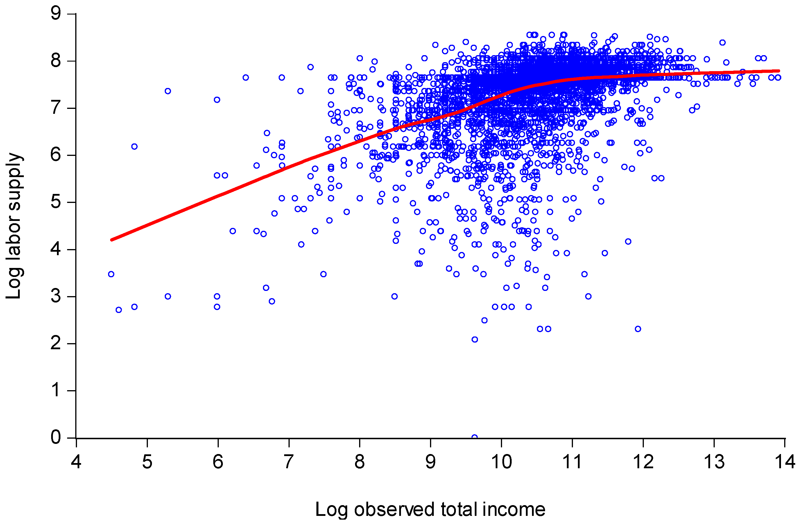
Labor supply is measured by average hours of work per week in 2013.28 The mean is 39 h (with a median is 40 h). The range in hours worked is from nearly zero to 99 h. Table 1 provides some key summary statistics and Figure 1 plots log hours worked per week in the last year against log total pre-tax income.29 Mean labor supply for those with an income under $20,000 (the poorest 16%) is 30 h, while it falls to 26 h for those living under $15,000 (the poorest 8%) (Table 1). We see that mean (log) labor supply rises with income up to a certain point then levels off for the upper 30% or so (Figure 1).
While there is an income gradient in labor supplies, it does not appear to be large enough to plausibly account for much of the income disparities. For example, the average hourly wage rate of those with income less than $20,000 is $8.26. Ten hours extra work at this wage rate would only make up 10% of the gap between the average income of this group and the overall mean income.30 Looked at a different way, this group of workers would have to work almost 100 h per week extra to reach mean income—equivalent to three full-time jobs. (Table 1 gives these calculations for various income cut-offs.)
While the income gradient in hours worked based on the regression function in Figure 1 does not seem especially steep, the pattern suggests that the partial effect of adjusting for effort as forgone leisure will go some way toward attenuating overall inequality in observed incomes. However, the large variance in labor supply at given income, especially at middle income levels evident in Figure 1 also comes into play. This “horizontal” effect is inequality increasing.
To see the net effect, consider first the measure of full income in which the standard for labor supply is set at 39 h. The assumption that the current wage can be maintained is questionable; to make up the hours, some may well have to switch to lower-paying jobs or incur prohibitively high personal costs of supplying the extra effort. So this simulation could well over-estimate the impact.
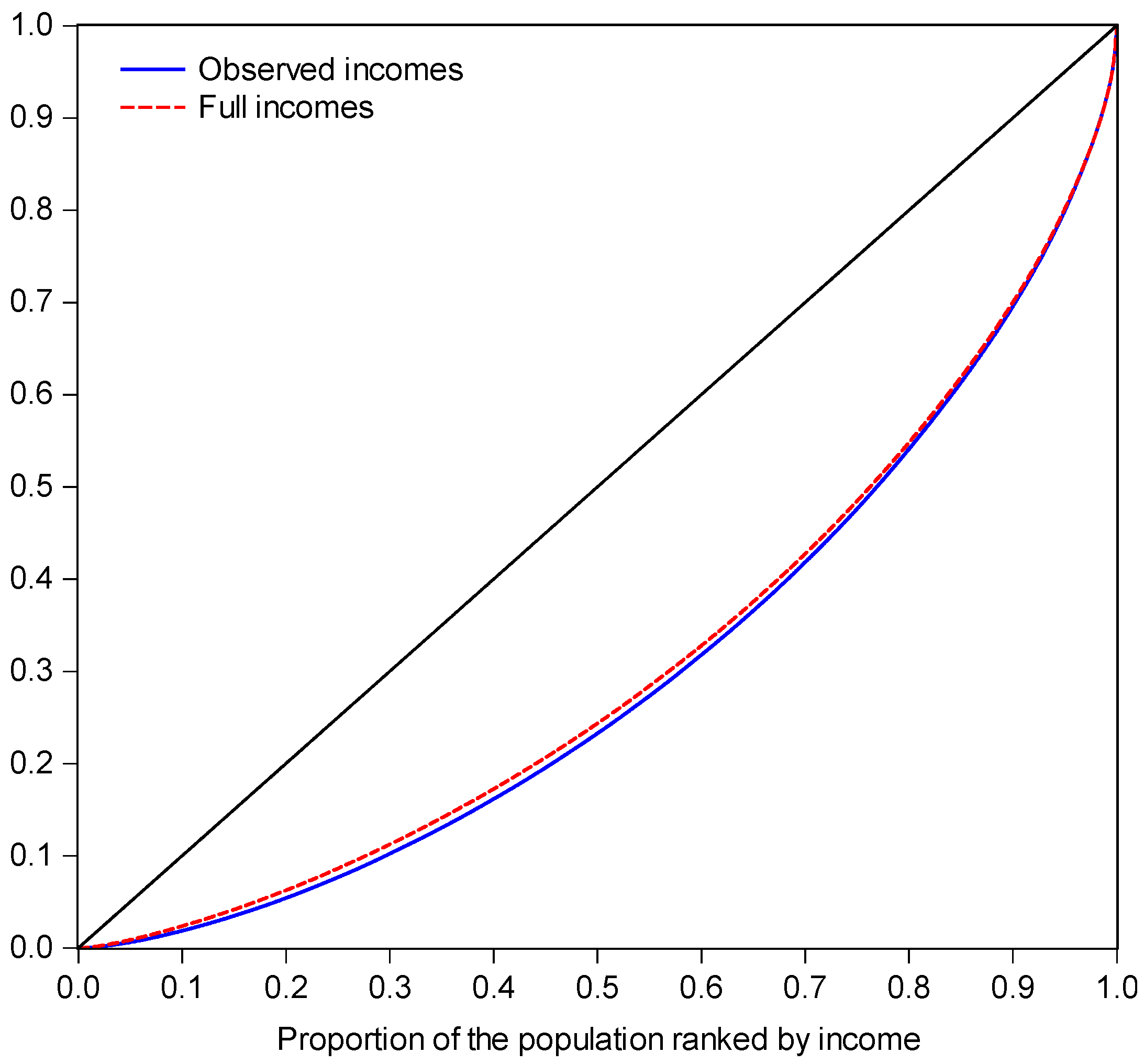
Figure 2 plots the full income against observed income (both in logs). There are some large proportionate gains, although they are spread through the income range. The first two rows of Table 2 give inequality measures for observed incomes and the full incomes. The full-time worker simulation brings down all three inequality measures. Figure 3 gives the Lorenz curves; there is not strict dominance, although the overlap does not happen until the 98th percentile.
When we come to incorporate effort in a welfare-consistent measure of income, this horizontal effect will again become important although then it will also interact with preferences. The net effect on measured inequality is thus an empirical issue to which we turn after describing the parametric model to be used.
Parametric model: In implementing an empirical model of income as a function of circumstances and effort the literature has often assumed a functional form that is additively-separable between effort and circumstances. However, it would clearly be questionable to assume that the marginal returns to circumstances are independent of effort. Indeed, in thinking about the economics one is drawn to postulate that the returns to effort (the wage rate when effort is simply labor supply) depend on circumstances—creating a natural interaction effect.
To consider the implications further, let us again write Equation (1) in the form of Equation (5). The values of w ( c i ) and π ( c i ) are the key parameters of effort choice. There are many possible assumptions one might make about preferences, and the results may well depend on the choice made. For the purpose of this example, a simple Cobb-Douglas representation is assumed, such that effort maximizes a utility function of the form:
u ( y i , x i , α i ) = ln y i + α i ln ( t x i )
where t is the total time available (so that t x i is leisure time). The heterogeneity in preferences is taken to be fully captured by the differences in the α i ’s. The (log) equivalent income is:
ln y i = ln y i + α i ln ( t x i t x ¯ )
Note that y i ( ) y i as x i ( ) x ¯ . Optimal labor supply requires α i = w ( c i ) ( t x i ) / y i ; the latter is called here the leisure ratio (the ratio of the imputed value of leisure to income). Mean labor supply of 39 h per week is used as the reference, though sensitivity to this choice is discussed below.
Comparison of the empirical income inequality measures: There are a number of possible scenarios of interest for the parameters and data. It may be expected that the presence of the relatively few low labor supplies in Figure 1 will exaggerate the extent of inequality in equivalent incomes. To address this concern the following analysis is restricted to those households who worked for money at least one day (8 h) per week on average over 2013. This cuts out about 200 households.31 The available time for work or leisure is set at 100, leaving out about 10 h per day. This seems reasonable.
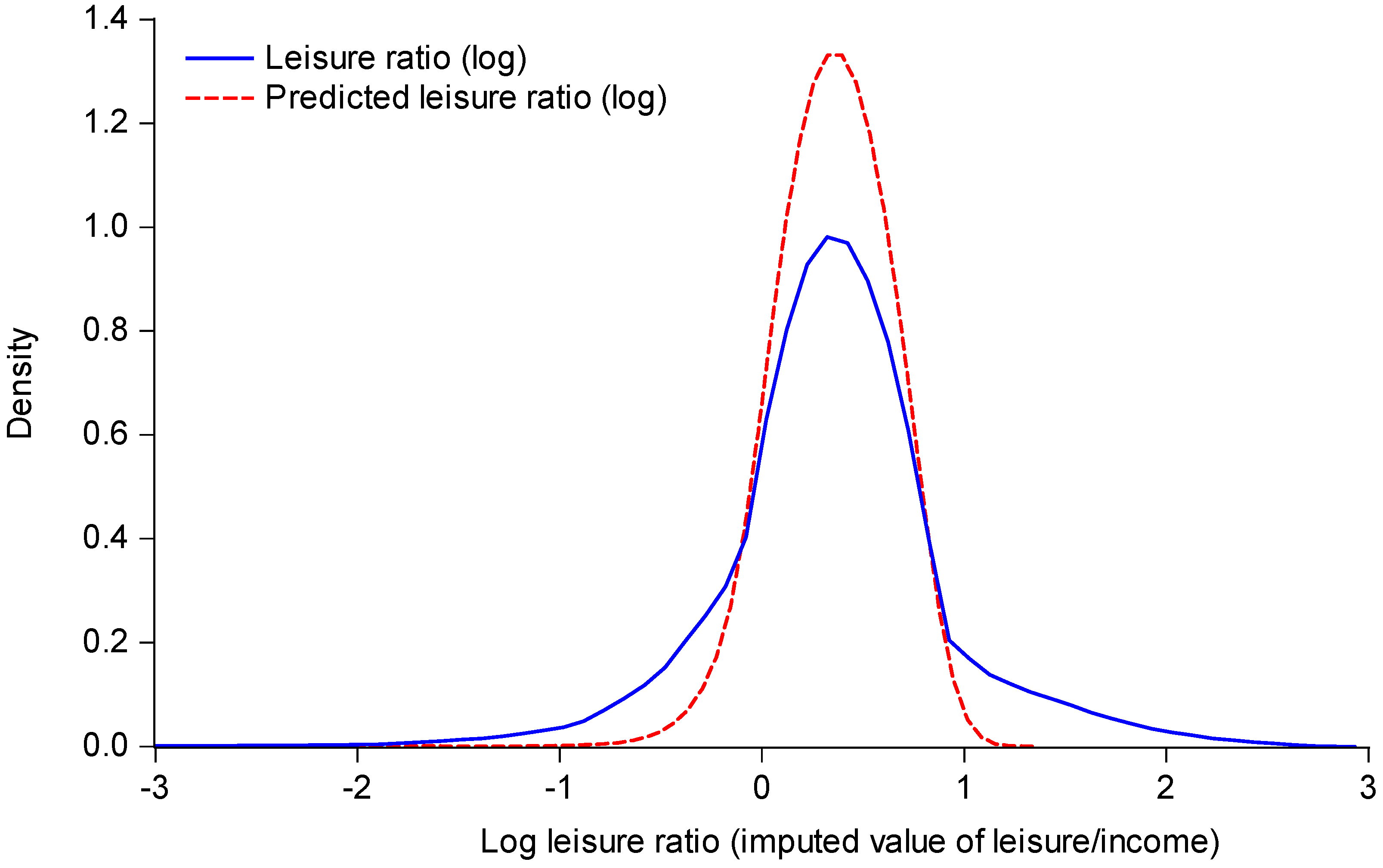
In allowing the preference parameter to vary, one possibility is to assume that everyone in the survey has freely chosen their ideal labor supply, and to set α i = w ( c i ) ( t x i ) / y i for all i. Results are given for this case, but it is questionable given the existence of labor-market frictions, whereby some survey respondents had too little leisure, and some too much, relative to their ideals. Setting the parameter to accord exactly with the leisure ratios in the survey data may be considered to produce an implausibly large variance. The spread of leisure ratios is evident in Figure 4. While the spread of empirical leisure ratios undoubtedly reflects labor-market frictions, measurement errors are also likely to be playing a role.
As an alternative, some degree of smoothing of the empirical leisure ratios is considered. For this purpose, the idiosyncratic preferences are set at the predicted values based on a regression of ln [ w ( c i ) ( t x i ) / y i ] on a quadratic function of the log wage rate, log unearned income (+$1) (with their interactions) and a vector of observed circumstances from the CPS related to gender, age, race, place of birth, whether parents were born in the U.S. (Unfortunately, the data source does not include other information about parents, such as their education.) Age enters as the deviation from the median of 49 years. The left-out group for the dummy variables comprises white, native-born, males of 49 years of age with parents born in the U.S.; 25% of the sample is in this group. The Appendix A Table A1 gives the regression for the leisure ratio. Figure 4 gives the densities of the predicted leisure ratio, showing how this trims the extreme values.
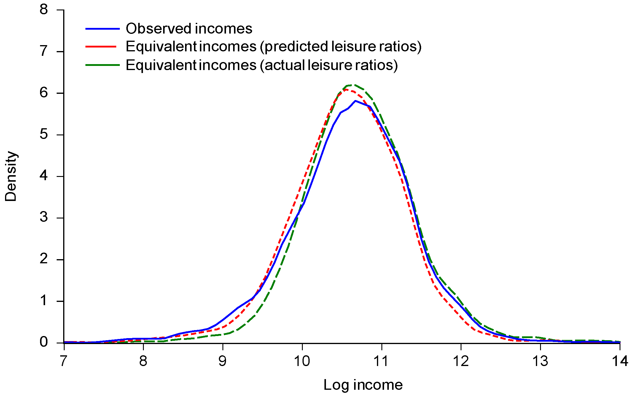
We can now calculate the equivalent incomes. Figure 5 gives the kernel density functions for log observed income and log equivalent income, using both the actual leisure ratios and the trimmed ratios (using the aforementioned predicted values). Using the trimmed preferences, the effect of the adjustment for effort is to attenuate both tails, and bring the mode down slight. Without the trimming (using actual leisure ratios) we only see the attenuation at the bottom tail (roughly speaking implying less poverty), though we still see the fall in the mode.
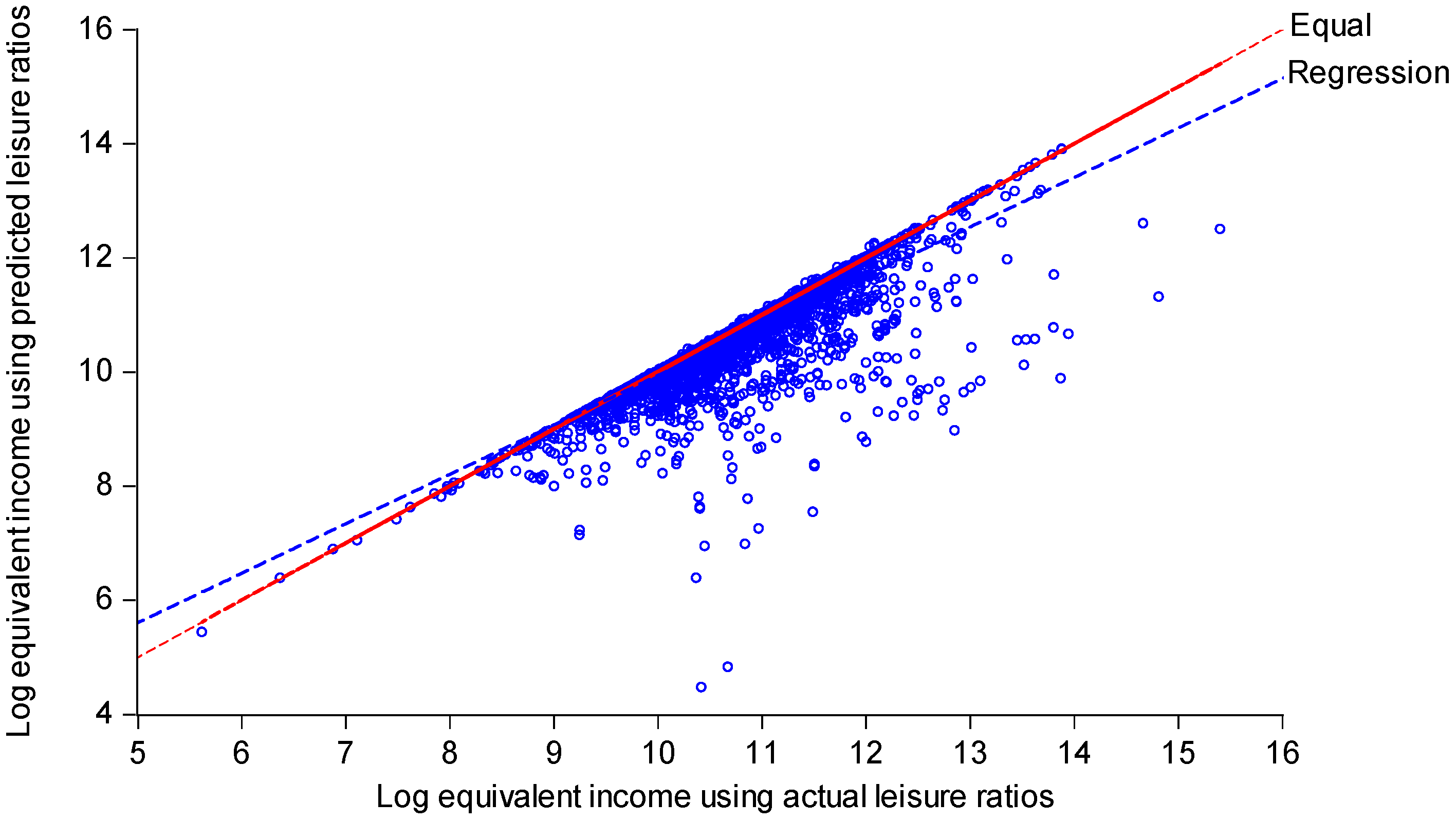
The effect of trimming the extremes in the preference parameter can be seen in Figure 6, which plots (log) equivalent income using the predicted leisure shares against those using the actual shares. As expected (based on Figure 4) there is a marked increase in the variance, especially around the middle. The Gini index rises to 0.421 (Table 2).
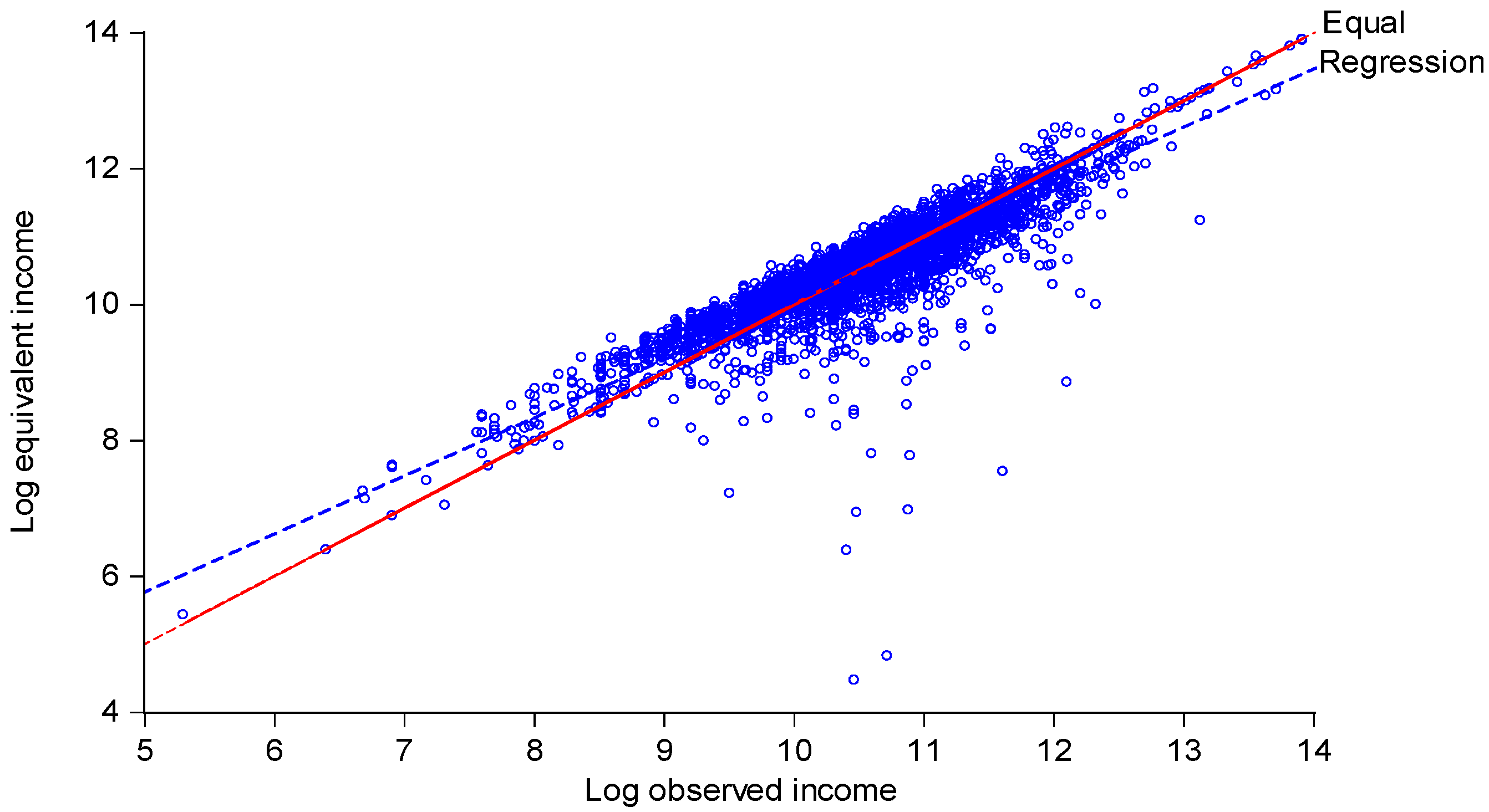
Figure 7 plots log equivalent income (using predicted leisure ratios) against log observed income. The Figure also gives the regression lines, which have slopes that are significantly less than unity.32 In other words, the adjustment for effort tends to raise (lower) equivalent incomes for the poor (rich). Equivalent incomes are also highly correlated with full incomes, again using a full-time job as the standard; in logs one finds that r = 0.924.
Table 2 also provides the same inequality indices for equivalent incomes and Figure 8 gives the Lorenz curves. On adjusting for effort without trimming the extremes of the preference parameters, the variance in the latter generates a marked outward shift in the Lorenz curve for the upper half; for the lower half the Lorenz curves are virtually indistinguishable, although there is not Lorenz dominance (so the ranking is not robust to the choice of inequality measure). The level of inequality falls when one adjusts for effort using the trimmed preference parameters. However, the effect is clearly very small.
As already noted, the choice of reference alters equivalent income. Lowering (increasing) the reference level of effort increases (reduces) measured inequality. For example, using x ¯ = 30 h per week (instead of the mean of 39) yields a Gini index for the equivalent incomes with trimming of 0.389. Using x ¯ = 50 h per week one gets a Gini index of 0.378.
Poverty measures: Table 3 gives poverty rates based on observed incomes for two illustrative income poverty lines, namely $15,000 and $20,000 per year. The poverty rates are 8% and 17% respectively. The table also gives the poverty rates using full income and equivalent income (with and without the trimming). Using the same nominal line, the poverty rates fall by similar amounts for full income and equivalent income without trimming, but bounce back to values very close to those for unadjusted incomes when the data are smoothed.
However, to calculate poverty rates based on equivalent incomes it is compelling to adjust the poverty line consistently with that metric of welfare (as discussed in the introduction). Table 3 also gives poverty rates for two indicative allowances for leisure as a basic need, namely 10 and 20 h per week, each valued at $7 per hour (the average wage of those with incomes under $15,000 per year). These are not particularly generous allowances; on average (in 2015), the U.S. population over 15 years spent 36 h per week in leisure activities (Bureau of Labor Statistics 2016). So the figure of 20 h is only a little more than half the mean. However, while these choices can be questioned, the aim here is to assess sensitivity to allowing for leisure as a basic need. Using the unsmoothed data, one finds that even a seemingly modest allowance for leisure as a basic need of a little over 10 h per week is enough to obtain higher poverty rates using equivalent incomes; at a basic need of 20 h of leisure per week, the poverty rates rise to 26% and 35% for basic lines of $15,000 and $20,000 respectively. For the smoothed data, even a very small allowance for leisure of two hours per week is sufficient to yield a higher poverty rate for equivalent incomes than observed incomes.33
Covariates of income: To throw some light on implications for the structure of inequality and poverty, Table 4 gives regressions of log observed income and log equivalent income (with and without trimming the preference parameters using the predicted leisure ratios) against the same set of variables describing circumstances used in predicting the leisure share. The regressions are very similar. The female income differential is halved when one adjusts for labor supply, though it remains significant.34 There are small differences in the effects of race and place of birth.35 Some of these effects may well be confounded by differences in unemployment rates by gender or race, and labor-market discrimination.

5. Conclusions

One often hears that high incomes are simply the reward for greater effort, and poverty reflects laziness, with the implication that there is less inequality and poverty than we think. Accepting that effort choice is a key factor in assessing inequality and that richer people tend to work more, this paper has shown that it is far from obvious that allowing for the disutility of effort implies less inequality or poverty.
If one takes seriously the idea that effort comes at a cost to welfare then it is clear that prevailing approaches are not using a valid monetary measure of welfare. While this much is obvious enough, the likely heterogeneity in effort must also be brought into the picture. Then the distributional outcome is far from obvious. It may be granted that average effort rises with income, but there is also a variance in effort at given income. The implications for measuring inequality and poverty stem from both the vertical differences (in how mean effort varies with income) and the horizontal differences (in how effort varies at given income).
It is unclear on a priori grounds what effect adjusting for effort in a welfare-consistent way will have on standard measures. There are both empirical and conceptual issues. The implications for measurement of taking effort seriously depend crucially on the behavioral responses to unequal opportunities, and not all of those responses are readily observable. Measures with a clearer welfare-economic interpretation call for data on efforts, for which existing surveys are limited to a subset of the dimensions of effort.
While acknowledging these limitations, the paper has provided illustrative calculations for American working singles without disabilities. A positive income gradient in labor supply is evident in the data. This gradient accounts for very little of the income gap between the poorest third (say) and the overall mean. The fact that poorer workers work less appears to contribute rather little to overall inequality in observed incomes. However, the considerable heterogeneity in effort at given incomes imparts a large horizontal element to inequality measures that adjust for effort consistently with behavior. On calculating distributions of welfare-consistent equivalent incomes to allow for this heterogeneity, the paper finds higher measures of inequality than for observed (unadjusted) incomes. Contrary to the common view, the prevailing practice of ignoring differences in effort understates inequality. It can be acknowledged, however, that some of the apparent heterogeneity in leisure preferences seen in the data is deceptive given likely rationing and measurement errors. When one smooths using predicted leisure shares based on covariates one finds a modest drop in the measured levels of inequality on adjusting for effort. Adjusting for effort does not appear to make much difference in the structure of inequality, as indicated by regressions using a set of circumstances related to gender, age, race and place of birth.
The implications for measures of poverty depend crucially on whether one sets the poverty line consistently with the welfare metric. If one does not do so, then poverty rates are lower using equivalent incomes although this essentially vanishes when one smooths the data. However, these comparisons are arguably deceptive since one is not setting the poverty line consistently with how one is assessing welfare. To correct for this, one needs to include a normative allowance for leisure as a basic need in setting the poverty line. On introducing even a modest allowance valued at a low wage rate, one finds higher poverty rates when one adjusts for effort. If half the average amount of leisure taken by American adults is deemed to be a basic need then the poverty rate based on equivalent incomes, adjusted for effort, is nearly twice as high as that based on observed incomes.
Whether one accepts all the assumptions underlying these calculations is an open question. However, it is clear from this study that it should not be presumed that allowing for effort in a way that is broadly consistent with behavior would substantially attenuate the disparities suggested by standard data sources on income inequality or poverty.

Acknowledgments

The comments of Tony Atkinson, Kristof Bosmans, Francois Bourguignon, Denis Cogneau, Quy-Toan Do, Raquel Fernandez, Francisco Ferreira, Garance Genicot, Jèrèmie Gignoux, Ravi Kanbur, Erwin Ooghe, John Rust, Elizabeth Savage, Dominique van de Walle and the journal’s two anonymous referees are gratefully acknowledged. The author thanks Naz Koont for very capable assistance in assembling the data files for Section 4.

Conflicts of Interest

The author declares no conflict of interest.

Appendix A

Table A1. Regression used to predict the leisure ratio to trim the extremes in allowing for idiosyncratic preferences.
Log Leisure Ratio
Coeff.SEProb.
Constant0.2560.0560.000
Log wage rate0.1500.0310.000
Log wage rate squared−0.0460.0050.000
Log unearned income (+1)−0.0730.0090.000
Log unearned income squared−0.0070.0010.000
Log wage x log unearned income0.0360.0020.000
Female0.0870.0150.000
Age-49 * 0.0000.0580.992
(Age-49) squared *0.0240.0030.000
Race: Black0.0750.0190.000
Race: Black mixed0.0870.0840.303
Race: American Indian0.0610.0660.355
Race: Asian0.0200.0520.705
Race: Other−0.0080.0580.885
Hispanic0.0630.0260.015
Born US Other Territories−0.1140.1520.452
Born Central America0.0370.1230.762
Born Caribbean−0.0420.1280.746
Born South America−0.1070.1380.438
Born Northern Europe−0.1610.1640.325
Born Western Europe−0.1080.1530.480
Born Central or Eastern Europe−0.1260.1360.352
Born East Asia0.0360.1360.789
Born SE Asia−0.0550.1420.698
Born SW Asia−0.1440.1500.337
Born Middle East−0.1360.1700.423
Born Africa−0.1740.1330.192
Foreign born0.0840.1160.472
Foreign: Dad−0.0280.0480.569
Foreign: Mom0.0230.0510.660
Foreign: Both−0.0420.0390.282
N5633
R20.122
S.E. of regression0.529
Mean dep. var.0.348
F-statistic25.962
Prob (F-statistic)0.000
Note: White standard errors (SE). * coefficients scaled up by 100.

References

  1. Allingham, Michael. 1972. The Measurement of Inequality. Journal of Economic Theory 5: 163–69. [Google Scholar] [CrossRef]
  2. Apps, Patricia, and Elizabeth Savage. 1989. Labour Supply, Welfare Rankings and the Measurement of Inequality. Journal of Public Economics 39: 335–64. [Google Scholar] [CrossRef]
  3. Atkinson, Anthony B. 1970. On the Measurement of Inequality. Journal of Economic Theory 2: 244–63. [Google Scholar] [CrossRef]
  4. Bargain, Olivier, Andre Decoster, Mathias Dolls, Dirk Neumann, Andreas Peichl, and Sebastian Siegloch. 2013. Welfare, Labor Supply and Heterogeneous Preferences: Evidence for Europe and the US. Social Choice and Welfare 41: 789–817. [Google Scholar] [CrossRef]
  5. Barros, Ricardo Paes de, Francisco H. G. Ferreira, J. Molinas Vega, and J. Saavedra Chanduvi. 2009. Measuring Inequality of Opportunities in Latin America and the Caribbean. Washington: The World Bank. [Google Scholar]
  6. Becker, Gary. 1965. A Theory of the Allocation of Time. The Economic Journal 75: 493–517. [Google Scholar] [CrossRef]
  7. Blundell, Richard, Costas Meghir, Elizabeth Symons, and Ian Walker. 1988. Labor Supply Specification and the Evaluation of Tax Reforms. Journal of Public Economics 36: 23–52. [Google Scholar] [CrossRef]
  8. Bourguignon, François. 2015. The Globalization of Inequality. Princeton: Princeton University Press. [Google Scholar]
  9. Bourguignon, François, Francisco Ferreira, and Marta Menéndez. 2007. Inequality of Opportunity in Brazil. Review of Income and Wealth 53: 585–618. [Google Scholar] [CrossRef]
  10. Browning, Martin. 1992. Children and Household Economic Behavior. Journal of Economic Literature 30: 1434–75. [Google Scholar]
  11. Brunori, Paolo, Francisco Ferreira, and Vito Peragine. 2013. Inequality of Opportunity, Income Inequality and Economic Mobility: Some international comparisons. In Getting Development Right. Edited by Eva Paus. New York: Palgrave Macmillan, chp. 5. [Google Scholar]
  12. Bureau of Labor Statistics. 2016. American Time Use Survey; Washington: United States Department of Labor.
  13. Champernowne, David, and Frank Cowell. 1998. Economic Inequality and Income Distribution. Cambridge: Cambridge University Press. [Google Scholar]
  14. Checchi, Daniele, and Vito Peragine. 2010. Inequality of Opportunity in Italy. Journal of Economic Inequality 8: 429–50. [Google Scholar] [CrossRef]
  15. Coles, Jeffrey L., and Paul Harte-Chen. 1985. Real Wage Indices. Journal of Labor Economics 3: 317–36. [Google Scholar] [CrossRef]
  16. Decoster, Andre, and Peter Haan. 2015. Empirical Welfare Analysis with Preference Heterogeneity. International Tax and Public Finance 22: 224–51. [Google Scholar] [CrossRef] [Green Version]
  17. Eichelberger, Erika. 2014. Debunking the Attempted Debunking of Our 10 Poverty Myths, Debunked. Mother Jones, March 28. [Google Scholar]
  18. Ferreira, Francisco, and Jèrèmie Gignoux. 2011. The Measurement of Inequality of Opportunity: Theory and an Application to Latin America. Review of Income and Wealth 57: 622–57. [Google Scholar] [CrossRef]
  19. Ferreira, Francisco, and Vito Peragine. 2015. Individual Responsibility and Equality of Opportunity. In Handbook of Well Being and Public Policy. Edited by M. Adler and M. Fleurbaey. Oxford: Oxford University Press. [Google Scholar]
  20. Ferreira, Francisco, Jèrèmie Gignoux, and Meltem Aran. 2011. Measuring Inequality of Opportunity with Imperfect Data: The Case of Turkey. Journal of Economic Inequality 9: 651–80. [Google Scholar] [CrossRef]
  21. Fleurbaey, Marc, and Vito Peragine. 2013. Ex Ante versus Ex Post Equality of Opportunity. Economica 80: 118–30. [Google Scholar] [CrossRef]
  22. Gans, Herbert. 1995. The War against the Poor. New York: Basic Books. [Google Scholar]
  23. Hassine, Nadia Belhaj. 2012. Inequality of Opportunity in Egypt. World Bank Economic Review 26: 265–95. [Google Scholar] [CrossRef]
  24. Jorgenson, Dale W., and Daniel Slesnick. 1984. Aggregate Consumer Behavior and the Measurement of Inequality. Review of Economic Studies 60: 369–92. [Google Scholar] [CrossRef]
  25. Kanbur, Ravi, and Michael Keen. 1989. Poverty, Incentives, and Linear Income Taxation. In The Economics of Social Security. Edited by Andrew Dilnot and Ian Walker. Oxford: Oxford University Press. [Google Scholar]
  26. Katz, Michael B. 1987. The Undeserving Poor: From the War on Poverty to the War on Welfare. New York: Pantheon Books. [Google Scholar]
  27. King, Mervyn A. 1983. Welfare Analysis of Tax Reforms Using Household Level Data. Journal of Public Economics 21: 183–14. [Google Scholar] [CrossRef]
  28. Marrero, Gustavo, and Juan Gabriel Rodriguez. 2012. Inequality of Opportunity in Europe. Review of Income and Wealth 58: 597–21. [Google Scholar] [CrossRef]
  29. Pencavel, John. 1977. Constant-Utility Index Numbers of Real Wages. American Economic Review 67: 91–100. [Google Scholar]
  30. Pew Research Center. 2014. Most See Inequality Growing, but Partisans Differ over Solutions. A Pew Research Center/USA TODAY Survey. Washington: Pew Research Center. [Google Scholar]
  31. Pignataro, Giuseppe. 2011. Equality of Opportunity: Policy and Measurement Paradigms. Journal of Economic Surveys 26: 800–34. [Google Scholar] [CrossRef]
  32. Pollak, Robert, and Terence Wales. 1979. Welfare Comparison and Equivalence Scale. American Economic Review 69: 216–21. [Google Scholar]
  33. Preston, Ian, and Ian Walker. 1999. Welfare Measurement in Labour Supply Models with Nonlinear Budget Constraints. Journal of Population Economics 12: 343–61. [Google Scholar] [CrossRef]
  34. Ramos, Xavier, and Dirk Van de gaer. 2016. Approaches to Inequality of Opportunity: Principles, Measures and Evidence. Journal of Economic Surveys 30: 855–83. [Google Scholar] [CrossRef]
  35. Ravallion, Martin. 2016. The Economics of Poverty. History, Measurement, Policy. New York: Oxford University Press. [Google Scholar]
  36. Roemer, John. 1998. Equality of Opportunity. Cambridge: Harvard University Press. [Google Scholar]
  37. Roemer, John E. 2014. Economic Development as Opportunity Equalization. World Bank Economic Review 28: 189–209. [Google Scholar] [CrossRef]
  38. Roemer, John, and Alain Trannoy. 2015. Equality of Opportunity. In Handbook of Income Distribution Volume 2. Edited by A. B. Atkinson and F. Bourguignon. Amsterdam: North Holland. [Google Scholar]
  39. Salverda, Weimer, Marloes de Graaf-Zijl, Christina Haas, Bram Lancee, and Natascha Notten. 2014. The Netherlands: Policy-Enhanced Inequalities Tempered by Household Formation. In Changing Inequalities and Societal Impacts in Rich Countries: Thirty Countries’ Experiences. Edited by Brian Nolan, Wiemer Salverda, Daniele Checchi, Ive Marx, Abigail McKnight, István György Tóth and Herman G. van de Werfhorst. Oxford: Oxford University Press. [Google Scholar]
  40. Singh, Ashish. 2012. Inequality of Opportunity in Earnings and Consumption Expenditure: The Case of Indian Men. Review of Income and Wealth 58: 79–106. [Google Scholar] [CrossRef]
  41. Slesnick, Daniel. 1998. Empirical Approaches to the Measurement of Welfare. Journal of Economic Literature 36: 2108–65. [Google Scholar]
  42. Stein, Ben. 2014. Poverty and Income Inequality. One really has Nothing to do with the Other. The American Spectator, April 4. [Google Scholar]
  43. Trannoy, Alain, Sandy Tubeuf, Florence Jusot, and Marion Devaux. 2010. Inequality of Opportunities in Health in France: A First Pass. Health Economics 19: 921–38. [Google Scholar] [CrossRef] [PubMed]
  44. Williamson, Kevin. 2014. Debunker Debunked. National Review, March 26. [Google Scholar]
1
As is well known, a source of ambiguity is that there are opposing income and substitution effects of higher wage rates on labor supply (assuming that leisure is a normal good). Higher unearned income will reduce work effort. The direction of the relationship with total income is unclear on theoretical grounds.
2
See, for example, Allingham’s (1972) comment on Atkinson (1970).
3
Of course, effort is only one aspect of the debates about inequality numbers; for example, there are also issues about price indices and equivalence scales. Note also that practitioners are on safer ground in measuring inequality amongst children for whom personal effort is not yet an issue. Here the concern is about inequality among adults.
4
This is an instance of a more general point that is well understood in welfare economics, namely that inequality of income need not imply inequality of welfare. Heterogeneity in preferences further complicates matters.
5
There have been a number of applications of the idea of money-metric utility to distributional analysis, including King (1983), Jorgenson and Slesnick (1984), Blundell et al. (1988), Apps and Savage (1989), Kanbur and Keen (1989). Also see the discussions in Slesnick (1998).
6
The economic arguments for assuring such consistency are reviewed in Ravallion (2016, Part 2).
7
This is an old idea, but in modern times it became prominent in Katz’s (1987) critique of American antipoverty policy. See Ravallion (2016, Part 1) on the history of economic thought on antipoverty policy. Also see Gans’s (1995, chp. 1) discussion of the history of derogatory labels for poor people.
8
For example, with reference to the U.S., Stein (2014) argues that: “There is an immense amount of income inequality here and everywhere. I am not sure why that is a bad thing. Some people will just be better students, harder working, more clever, more ruthless than other people”. Stein goes on to claim that long-term poverty reflects “poor work habits”. Also see the debate between Eichelberger (2014) and Williamson (2014) on the proposition that “poor people are lazy”.
9
Champernowne and Cowell (1998) only give passing reference to the idea, and do not develop its implications. Kanbur and Keen (1989) discuss its use in the context of inequality and taxation. The concept of “full-time equivalent income” is found in business and labor studies; see, for example, the online Business Dictionary.
10
This is not the same concept of full income found in Becker (1965), which includes the imputed value of the entire time endowment.
11
This is shown by Kanbur and Keen (1989) in the context of heterogeneous effort though the point is more general.
12
The measures include Pencavel’s (1977) real wage metric, given by wage rate equivalent of the actual utility level at fixed values of other factors, including unearned income, and an analogous “rent metric” given by the unearned income equivalent of utility. A useful overview of the various measures possible can be found in Preston and Walker (1999). An earlier empirical application of the real wage index idea can be found in Coles and Harte-Chen (1985).
13
14
This is sometimes called “ex-ante” equality; “ex-post” equality requires equal reward for equal effort; see the discussion in Fleurbaey and Peragine (2013). For example, if someone starting out with a disadvantage in terms of her ability to generate income can make up the difference by hard work then one would surely be reluctant to say that there is no remaining inequality of opportunity; while the income difference according to circumstances may have vanished (no ex ante inequality), the difference in welfare remains (ex post inequality).
15
This is explicit in Bourguignon et al. (2007), Trannoy et al. (2010) and Ferreira and Gignoux (2011), but implicit in most of the literature. Ferreira and Peragine (2015) claim that the method has been applied to at least 40 countries.
16
Effort is bounded, but this is not made explicit for now since attention is confined to interior solutions for effort. (In the parametric model in section 4 a time constraint will be explicit.)
17
Subscripts for person i are dropped in places to simplify the notation. Twice differentiability is assumed when convenient. Subscripts are used for partial derivatives, in obvious notation. When convenient for the exposition, c and x are treated as continuous scalars (such as parental income and labor supply respectively), but they are vectors in reality and with discrete elements.
18
Notice that this model is static, in that all effort is a current choice. In extending to a dynamic model one might postulate that there are also current gains from past efforts, which are taken as exogenous to choices about current effort. (An example is past effort at school versus current labor supply given schooling.)
19
This is explicit in Bourguignon et al. (2007), Trannoy et al. (2010) and Ferreira and Gignoux (2011), but implicit in most of the literature.
20
Of course, in practice ε also includes unobserved circumstances and measurement errors. A discussion of the econometric issues in specifying and estimating Equation (4) can be found in Ramos and Van de gaer (2016).
21
A similar comment applies to the use of the wage rate as a metric of welfare.
22
In obvious notation and subsuming x ¯ in the definition of the equivalent-income function f.
23
The interior points on the income Lorenz curve, L(p), are L(1/3) = 0.25 and L(2/3) = 0.5, while those for the welfare Lorenz curve are L(1/3) = (1 − α)/(4 − 2α) < 0.25 and L(2/3) = 0.5. (Note that the two people with lowest incomes are re-ranked when one switches to the welfare space.)
24
This claim uses the well-known Lorenz dominance condition (Atkinson 1970).
25
This assumes a common poverty line; the empirical work will relax this to allow for leisure as a basic need.
26
This relates to the long-standing problem of inferring welfare from observed demand or supply behavior across demographically heterogeneous households (Pollak and Wales 1979; Browning 1992).
27
The CPS data were accessed through the University of Minnesota’s IPUMS-CPS site.
28
This is obtained by multiplying reported weeks of work in the last year by reported average hours of work per week then dividing by 52.
29
Recall that pre-tax income (y) is the relevant concept in the model in Section 2 in which taxes are solved-out, assuming that they are some function of y. Also note that the CPS does not ask for taxes paid so imputations of uncertain reliability are required.
30
The overall mean weekly income of the sample is $1048, while the mean weekly income of those living below $20,000 per annum is $245.
31
As noted, those reporting any disability affecting work or any difficulty (seeing, hearing, remembering, mobility, personal care) are excluded from the main analysis reported here. 5% of the sample reported a disability affecting their work.
32
The regression coefficient is 0.856 (White s.e. = 0.006).
33
With two hours per week of leisure the poverty rate using the smoothed data is 9.1% using the $15,000 income line and 16.9% using $20,000.
34
The data do not include work done within the home, though this is probably similar by gender in the sample of single adults.
35
For example, the negative income effects of being born in South America or Center-Eastern Europe become somewhat larger (and statistical significant) using equivalent incomes based on the actual leisure ratios.
Figure 1. Labor supply plotted against total income for U.S. single adults in 2013. Note: The regression line is the “nearest neighbor” smothered scatter plot using a locally-weighted quadratic function. The overall quadratic regression (with White standard errors in parentheses) is: ln x i = 6.873 ( 0.994 ) + 1.712 ( 0.143 ) ln y i 0.069 ( 0.009 ) ln y i 2 + ε ^ i R 2 = 0.206 ;   n = 5863 .
Econometrics 05 00050 g001
Figure 2. Plot of full incomes against observed incomes. Note: The full incomes are calculated by assuming that all those working less than average hours were to work average hours at the same wage rate as at present.
Econometrics 05 00050 g002
Figure 3. Lorenz curves for observed incomes and “full-employment” incomes.
Econometrics 05 00050 g003
Figure 4. Kernel densities of the log leisure ratio.
Econometrics 05 00050 g004
Figure 5. Kernel density functions for log incomes.
Econometrics 05 00050 g005
Figure 6. Effect of trimming the preference parameters.
Econometrics 05 00050 g006
Figure 7. Plot of log equivalent income against log observed income. Note: Equivalent incomes based on predicted leisure ratios.
Econometrics 05 00050 g007
Figure 8. Lorenz curves for observed and equivalent incomes.
Econometrics 05 00050 g008
Table 1. Summary statistics.
Income Cut-off (z)% of SampleMean Hours of Work per Week ( h ¯ z )Mean Wage Rate ($/Hour) ( w ¯ z )Mean Income ($/Week) ( y ¯ z )% of Income Gap Covered by Working Average Hours per Week ( 100 ( 39.26 h ¯ z ) w ¯ z ( 1048.26 y ¯ z ) )Extra Hours per Week to Reach Mean Income ( 1048.26 y ¯ z w ¯ z )
10,0004.0323.665.62119.159.44165.32
15,0008.3126.357.10177.2010.52122.68
20,00015.1129.568.26244.969.9797.25
25,00022.6731.649.38304.609.6179.28
30,00029.6633.0010.28354.909.2867.45
35,00038.2034.5011.40411.698.5255.84
Median50.0035.8112.92487.847.9543.38
Maximum100.0039.2624.091048.26n.a.0.00
Note: The median is $42,010. Means are calculated for all sample points up to z.
Table 2. Inequality measures for U.S. working singles without disabilities.
Income ConceptGini Index Mean Log Deviation (MLD)Robin Hood Index
Observed income0.4020.2960.284
Full income 0.3870.2620.275
Equivalent income without trimming extreme values0.4210.3100.299
Equivalent income trimming extreme values 0.3850.2720.272
Note: Full incomes are calculated by assuming that all those working less than the mean hours of 39 per week were to work those hours at the same wage rate as at present. The equivalent incomes are explained in the text. The Gini index is half the average absolute difference between all pairs of incomes, expressed as a proportion of the mean. MLD is given by the mean of the log of the ratio of the overall mean income to individual income. Robin Hood index is the maximum vertical difference between the diagonal and the Lorenz curve, interpretable as the fraction of total income that one would need to take away from the richer half and give to the poorer half to assure equality.
Table 3. Poverty measures for U.S. working singles without disabilities.
Income Poverty Line
$15,000$20,000
Observed income0.0830.165
Full income 0.0460.115
Equivalent income without trimming extreme values
No basic need for leisure 0.0450.103
Basic need = 10 h/week0.0810.155
Basic need = 20 h/week0.1290.216
Equivalent income trimming extreme values
No basic need for leisure 0.0820.158
Basic need = 10 h/week0.1330.219
Basic need = 20 h/week0.1910.283
Note: The basic need for leisure is valued at $7 per hour. The poverty lines allowing for a basic need for leisure of 10 h per week are $18,640 (for the $15,000 income poverty line) and $23,640 (for $20,000). Allowing for a basic need for leisure of 20 h per week the corresponding lines are $22,280 and $27,280. (Also see notes to Table 2.)
Table 4. Testing for inequality of opportunity for U.S. working singles without disabilities.
(1)(2)(3)
Log Observed IncomeLog Equivalent Income
(Predicted Leisure Ratios)
Log Equivalent Income
(Actual Leisure Ratios)
Coeff.s.e.Prob.Coeff.s.e.Prob.Coeff.s.e.Prob.
Constant10.8420.0190.00010.7270.0190.00010.8470.0180.000
Female−0.1070.0210.000−0.0530.0200.007−0.0540.0190.005
Age-49 * 0.0070.0010.0000.0080.0010.0000.0080.0010.000
(Age-49) squared *0.0000.0000.0000.0000.0000.0000.0000.0000.057
Race: Black−0.2240.0260.000−0.1820.0240.000−0.1890.0240.000
Race: Black mixed−0.1420.1170.223−0.0830.1050.427−0.1080.1090.321
Race: Am. Indian−0.2610.0860.002−0.2270.0790.004−0.2210.0810.007
Race: Asian0.1520.0690.0280.1490.0630.0190.1980.0650.002
Race: Other−0.0830.0970.389−0.1060.0870.225−0.1030.0890.251
Hispanic−0.1620.0370.000−0.1340.0360.000−0.1270.0340.000
Born US Oth.Terr.−0.1380.2470.577−0.1450.2230.514−0.2840.2060.168
Born Central Am.−0.7240.1970.000−0.6680.1760.000−0.6670.1570.000
Born Caribbean−0.4350.2030.032−0.4300.1830.019−0.4740.1660.004
Born S. America−0.3110.2150.149−0.3420.1960.082−0.4380.1780.014
Born N. Eur.0.2290.2350.3310.1860.2090.3750.0660.1920.731
Born Western Eur.−0.0520.2760.850−0.1180.2480.633−0.1200.2410.618
Born C-East Eur.−0.2490.2060.226−0.3000.1840.103−0.4100.1630.012
Born East Asia−0.3140.2120.139−0.2840.1900.134−0.3090.1750.078
Born SE Asia−0.5480.2280.016−0.5940.2120.005−0.6550.1910.001
Born SW Asia−0.1430.2260.526−0.2100.2130.326−0.2990.1860.108
Born Middle East0.0960.2670.719−0.0210.2460.9320.0880.2440.717
Born Africa−0.1850.2040.365−0.2830.1850.127−0.3020.1710.077
Foreign born0.2600.1870.1650.2890.1670.0840.3320.1480.025
Foreign: Dad0.1060.0590.0730.0870.0560.1170.0830.0580.152
Foreign: Mom0.1580.0740.0340.1730.0620.0060.2280.0680.001
Foreign: Both0.1320.0560.0180.1190.0510.0200.0870.0500.083
N5633 5633 5633
R20.088 0.077 0.068
S.E. of regression0.750 0.714 0.698
Mean dep. var.10.610 10.569 10.724
F-statistic21.740 18.600 16.373
Prob (F-statistic)0.000 0.000 0.000
Note: White standard errors (s.e.). * coefficients scaled up by 100.