Top Incomes, Heavy Tails, and Rank-Size Regressions

Abstract

In economics, rank-size regressions provide popular estimators of tail exponents of heavy-tailed distributions. We discuss the properties of this approach when the tail of the distribution is regularly varying rather than strictly Pareto. The estimator then over-estimates the true value in the leading parametric income models (so the upper income tail is less heavy than estimated), which leads to test size distortions and undermines inference. For practical work, we propose a sensitivity analysis based on regression diagnostics in order to assess the likely impact of the distortion. The methods are illustrated using data on top incomes in the UK.

1. Introduction

Income distributions exhibit, like many other size distributions in economics and the natural science, upper tails that decay like power functions (see e.g., Schluter and Trede 2017). The recent and rapidly growing literature on top incomes focuses on this upper tail, and its presence has important consequences for the measurement of inequality.1 However, estimating the heaviness of the upper tail is challenging, since real world size distributions usually are Pareto-like (i.e., tails are regularly varying) rather than strictly Pareto.

To be precise, let $X_1,\dots ,X_n$ be a sequence of positive independent and identically distributed random variables (e.g., incomes) with distribution function F that is regularly varying, so for large x

$$1-F\left(x\right)=x^{-\frac{1}{\gamma }}l\left(x\right),\gamma \in (0,\infty ),$$

(1)

where l is slowly varying at infinity, i.e., $l\left(tx\right)/l\left(x\right)=1$ as $x\to \infty$. The parameter $\gamma$, usually referred to as extreme value index (and $1/\gamma$ as the tail exponent), is unknown and needs to be estimated. Many estimators have been proposed in the statistical literature (see e.g., the textbook treatments in (Embrechts et al. 1997 or Beirlant et al. 2004).

An estimator popular among economists is based on a simple ordinary least squares (OLS) regression of log sizes on log ranks (e.g., Jenkins 2017 and Atkinson 2017, and references therein, in the income distribution and top incomes literature, this regression is ubiquitous in the city size literature). The enduring popularity of the OLS estimator is partly due to its simplicity, and partly due to a powerful intuition based on a Pareto quantile-quantile (QQ)-plot, the regression estimating its slope coefficient. However, if the tail of the distribution varies regularly, the Pareto QQ-plot will become linear only eventually. In particular, (1) can be expressed equivalently, using the tail quantile function $U\left(x\right)=\inf \{t:\mathrm{Pr}(X>t)=1/x\}$ where $x>1$, as $U\left(x\right)=x^{\gamma }\tilde{l}\left(x\right)$ where $\tilde{l}\left(x\right)$ is a slowly varying function. Hence, as $x\to \infty$, $\log U\left(x\right)\sim \gamma \log \left(x\right)$ since then $\log \tilde{l}\left(x\right)\to 0$. Replacing these population quantities with their empirical counterparts gives the Pareto QQ-plot, and $\gamma$ is its ultimate slope. This qualification (usually ignored by practitioners in economics) has important consequences for the behaviour of the estimator: Since the OLS estimator estimates the slope parameter of this QQ-plot, deviations from the strict Pareto model -captured by the nuisance function l- will induce distortions.

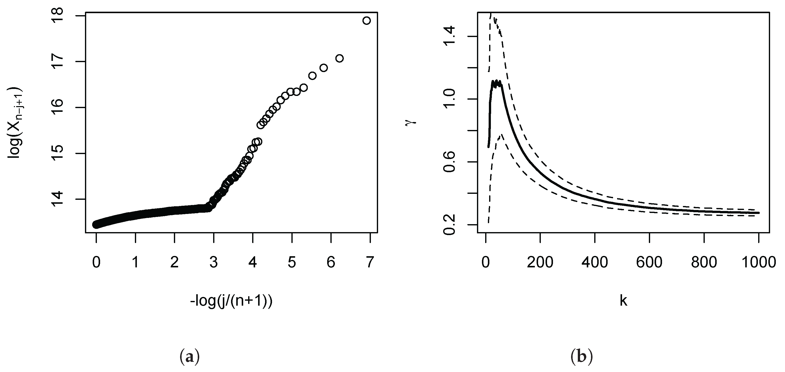
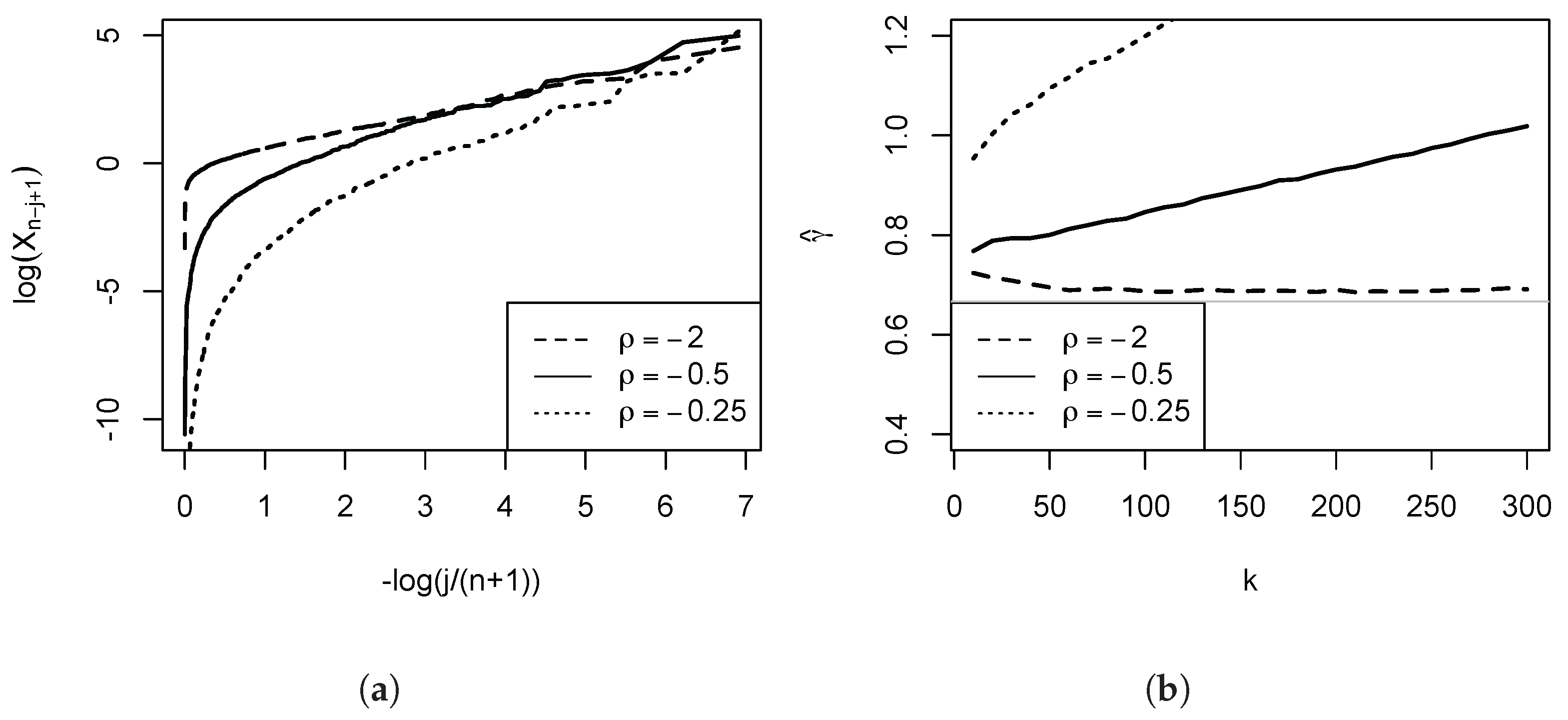
The empirical importance of this is illustrated in Figure 1, which depicts the Pareto QQ-plot for our administrative income data for the UK (the subject of our empirical application developed in Section 4 below), using the 1000 largest incomes. The plot exhibits a pronounced kink, and approximate linearity of the QQ-plot only holds for the very highest upper order statistics. Panel (b) shows the consequences for the OLS estimates: As we move in the QQ-plot from the right to the left, the departures from linearity become progressively more severe, and the OLS estimates progressively fall. Based on this first diagnostic QQ-plot, once the lower upper order statistics have been discarded as a source of downward bias, the subsequent analysis can then more clearly focus on the approximate linear part, the remaining distortions, and the choice of the number of order statistics. Figure 2 provides a further illustration for three Burr (Singh-Maddala) distributions (examined in detail in Section 3 below, being the leading parametric income distribution model) possessing the same $\gamma$. Here, the speed of decay of the nuisance function l is parametrised by the absolute value of the parameter $\rho$. The smaller the magnitude of $\rho$, the greater the initial curvature and steepness of the Pareto QQ-plot, and the larger the induced positive distortions of the OLS estimator of the slope coefficient.

In this paper, we examine the asymptotic distortions of the OLS estimator that arise in these circumstances, caused by the slow decay of the nuisance function l and modeled here as higher order regular variation. The theory is presented in Section 2 (proofs are collected in Appendix A), and numerical illustrations and quantifications of the distortions are provided in Section 3, as well as of the stark consequence for inference. More specifically, we show formally that the OLS estimator over-estimates the true value in the leading heavy-tailed model (i.e., the Hall class, which includes the Burr (Singh-Maddala) distribution, as well as the student, Fréchet, and Cauchy distributions). An empirical illustration in the context of top incomes in the UK using data on tax returns is the subject of Section 4.

1.1. The Log-Log Rank-Size Regression

We briefly review the rank size regression. Let $X_{1,n}\le \cdots \le X_{n,n}$ denote the order statistics of $X_1,\cdots ,X_n$, and consider the k upper order statistics. Let ranks be shifted by a constant $\eta <1$. The regression of sizes on ranks leads to the minimisation of the least squares criterion

$$\sum _{j=1}^k{\left(\log \frac{X_{n-j+1,n}}{X_{n-k,n}}-g\log \frac{k+1}{j-\eta }\right)}^2$$

(2)

with respect to g, where $\eta <1$ and $1\le j\le k<n$. The classic case is $\eta =0$. However, since the OLS estimator of the slope coefficient is not invariant to shifts in the data, it is conceivable that a purposefully chosen shift could yield an asymptotic refinement (Gabaix and Ibragimov 2011 consider this in the strict Pareto model $1-F\left(x\right)=c{x}^{-1/\gamma }$). The analysis below allows for this possibility.

The justification of considering regression (2) is based on a Pareto QQ-plot (Beirlant et al. 1996): For a sufficiently high threshold $X_{n-k,n}$ where $k<n$, the Pareto quantile plot in model (1) with coordinates $(-\log (j/(n+1)),$ $\log X_{n-j+1,n}{)}_{j=1,\cdots ,k}$ becomes ultimately linear. The line through point $-\log \left(\right(k+1)/(n+1\left)\right),$ $\log X_{n-k,n})$ with slope g is thus given by $y=\log X_{n-k,n}+g[x+\log ((k+1)/(n+1))]$ and the data points are $(x,y)=(-\log (j/(n+1)),$ $\log X_{n-j+1,n}{)}_{j=1,\cdots ,k}$. The regression estimator estimates this slope parameter. In particular, the OLS estimator of the slope coefficient g is

$$\begin{array}{ccc}\hfill \widehat{\gamma }& =& \frac{\frac{1}{k}{\sum }_{j=1}^k\log \left(\frac{k+1}{j-\eta }\right)\left[\log X_{n-j+1,n}-\log X_{n-k,n}\right]}{\frac{1}{k}{\sum }_{j=1}^k{\left[\log \frac{k+1}{j-\eta }\right]}^2}\equiv \frac{N_{n,k}}{D_k},\eta <1.\hfill \end{array}$$

(3)

Note that the denominator $D_k$ is a Riemann approximation to ${\int }_0^1{\log }^{2}x\mathrm{d}x=2$. An asymptotic expansion of the denominator reveals that

$$D_k=2+O\left(\frac{{\log }^{2}k}{k}\right)$$

(4)

From Kratz and Resnick (1996, proof of their Equation 2.4, p. 704) we know that the numerator $N_{n,k}$ converges in probability to $2\gamma$, hence the estimator is weakly consistent: $\widehat{\gamma }{\to }^P\gamma$ as $k\to \infty$ and $k/n\to 0$. We proceed in the next Section to refine this result by obtaining higher order expansions of the estimator in (3).

The literature contains several variants of regression (2). Rather regressing log sizes on log ranks, one could regress log ranks on log sizes, thus obtaining the ‘dual’ regression. In view of (3), our asymptotic analysis of the numerator carries immediately over to this dual regression. Another variant of (2) includes the additional estimation of a regression constant: $\log X_{n-j+1,n}$ is regressed on a constant and $\log j$. Kratz and Resnick (1996) obtain the distributional theory for this alternative estimator and show that its asymptotic variance is $2{\gamma }^2/k$, which exceeds, as will be shown below, the asymptotic variance of $\widehat{\gamma }$ given by (3). Hence this regression variant is less efficient. Schultze and Steinebach (1996) also prove weak consistency of the estimator in this setting.

2. Asymptotic Expansions and Distributional Theory

2.1. Preliminaries: Higher Order Regular Variation

In order to obtain our asymptotic expansions, we use an equivalent representation of model (1) based on regular variation and extreme value theory. First we recall the definition of first-order regular variation, and then proceed to model the slowly varying nuisance function l in (1) by a refinement to second-order regular variation. We then show that most heavy-tailed distributions of interest (in the income, finance and urban literature) satisfy this condition.

It is well known that model (1) has the equivalent (first-order regular variation) representation (e.g., Dekkers et al. 1989)

$$\underset{t\to \infty }{\lim }\frac{\log U\left(tx\right)-\log U\left(t\right)}{a\left(t\right)/U\left(t\right)}=\log x,$$

(5)

for all $x>0$ where a is a positive norming function with the property $a\left(t\right)/U\left(t\right)\to \gamma$. The problem for estimating the extreme value index $\gamma$ is the behaviour of the slowly varying function l in (1). It is, therefore, common practice in the extreme value literature to model such second-order behaviour, thus strengthening model (1), by strengthening the first-order regular representation (5) to second-order regular variation. Following De Haan and Stadtmüller (1996), we assume that the following refinement of (5) holds

$$\underset{t\to \infty }{\lim }\frac{\frac{\log U\left(tx\right)-\log U\left(t\right)}{a\left(t\right)/U\left(t\right)}-\log x}{A\left(t\right)}=H_{\gamma ,\rho }\left(x\right)$$

(6)

for all $x>0$, where $H_{\gamma >0,\rho <0}\left(x\right)=\frac{1}{\rho }(\frac{x^{\rho }-1}{\rho }-\log x)$ with $\rho <0$. This parameter $\rho$ is the so-called second-order parameter of regular variation, and $A\left(t\right)$ is a rate function that is regularly varying with index $\rho$, with $A\left(t\right)\to 0$ as $t\to \infty$. As $\rho$ falls in magnitude, the nuisance part of l in (1) decays more slowly. Our numerical illustrations will thus consider small magnitudes for $\rho$.

Examples. 

Most heavy-tailed distributions of interest satisfy representation (6). Consider the Hall class of distributions (Hall 1982), given by, for large x,

$$F\left(x\right)=1-a{x}^{-1/\gamma }[1+b{x}^{\beta }+o\left(x^{\beta }\right)]$$

with $\gamma ,a>0$, $b\in R$, $\beta <0$. In this class, the nuisance function l in model (1) converges to a constant at a polynomial rate. The Hall class nests, for instance, the Burr (Singh-Maddala), Student, Fréchet, and Cauchy distributions.2 The tail quantile function is $U\left(x\right)=c{x}^{\gamma }[1+d{x}^{\rho }+o\left(x^{\rho }\right)]$ where $c=a^{\gamma }$, $d=b\gamma a^{\gamma \beta }$. This Hall class satisfies the second order representation (6) with $\rho =\gamma \beta <0$, and rate function

$$A\left(t\right)=\frac{{\rho }^2}{\gamma }d{t}^{\rho }.$$

Figure 2 illustrates the role of $\rho$ for the Burr distribution (examined in greater detail in Section 3) in terms of the Pareto QQ-plot, and the implications for the estimator $\widehat{\gamma }$ of its slope parameter. For $\rho =-2$ the plot is close to linear, and the estimates close to the population value. However, as $\rho$ falls in magnitude, the initial curvature increases, and the slope estimates consequently becomes more positively distorted as the number of upper order statistics k entering the estimator increases.

2.2. The Main Results

We first state the higher order asymptotic expansion of the numerator $N_{n,k}$. We then obtain the distributional theory for our estimator $\widehat{\gamma }$, before returning to the distortions induced by deviations from the strict Pareto model (captured by second order regular variation).

Asymptotic expansion.

In the Appendix A we prove the following higher order expansion of the numerator $N_{n,k}$ under the assumption of second-order regular variation (6). Throughout, we will consider an intermediate sequence $k=k_n$ of positive integers such that $k_n\to \infty$ and $k_n/n\to 0$ as $n\to \infty$. It is then true that, for $\gamma >0$ and $\rho <0$,

$$\begin{array}{ccc}\hfill N_{n,k}/\gamma & =& 2-\left(\frac{1}{2}-\eta \right)\frac{\log (k-\eta )}{k}-\left(\frac{1}{2}-\eta \right)\frac{{\log }^{2}k}{2k}\hfill \\ & +& O_p\left(\frac{1}{k^{1/2}}\right)+O\left(\frac{1}{k}\right)+O_p\left(\frac{\log k}{k^{1/2}}\right)\hfill \\ & +& A\left(\frac{n}{k}\right)\frac{1}{\rho }\left[\frac{2-\rho }{{(1-\rho )}^2}\right]+O_p\left(\frac{\log k}{k}\right)+o_p\left(A(n/k)\right)\hfill \end{array}$$

(7)

A few comments are in order. The first two lines of this expression characterise the first-order behaviour of the numerator. It can be seen that setting the regression shift factor $\eta$ to 1/2 eliminates the second and third term. However, the term $O_p\left(\log k/k^{1/2}\right)$ is still present. The asymptotic refinement due to second-order regular variation is given by the terms of line 3. Although $A\left(t\right)\to 0$ as $t\to \infty$, this decay might be slow: $A\left(t\right)$ is regularly varying with index $\rho$, and as $\rho$ falls in magnitude the nuisance part of l in (1) decays more slowly. A slow decay then introduces a noticeable distortion in finite samples. We examine these distortions after stating the distributional theory for the estimator.

Distributional theory.

Beirlant et al. (1996) observe that our slope estimator $\widehat{\gamma }$, given by (3), is (to first order) a member of the class of kernel estimators discussed in Csorgo et al. (1985) with kernel $K\left(t\right)=1-\log t$. Since ${\int }_0^{1}K\left(t\right)\mathrm{d}t=2$ and not unity, a scale correction is required. Since ${\int }_0^1{K}^2\left(t\right)\mathrm{d}t=5$, the following result obtains as $k\to \infty$ and $k/n\to 0$, and if $\sqrt{k}A(n/k)\to 0$

$$\sqrt{k}(\widehat{\gamma }-\gamma ){\to }^{d}N\left(0,\frac{5}{4}{\gamma }^2\right)$$

(8)

Higher order distortions.

Asymptotically, the estimator is thus unbiased if $\sqrt{k}A(n/k)\to 0$. If this decay is slow, however, the estimator will suffer from a higher order distortion in finite samples. By (7), this distortion equals, for $\gamma >0$ and $\rho <0$,

$$b_{k,n}\equiv \frac{1}{2}\frac{\gamma }{\rho }\frac{2-\rho }{{(1-\rho )}^2}A(n/k)$$

(9)

In particular, in the Hall model, $A\left(t\right)=({\rho }^2/\gamma )d{t}^{\rho }$. The sign of the higher order distortion of $N_{n,k}$ and hence $\widehat{\gamma }$ is, since $\rho <0$, then given by -sgn$\left(d\right)$. For the Burr (Singh-Maddala), student, Fréchet, and Cauchy distributions it can be shown that $d<0$, leading to a positive higher order distortion. We conclude that the higher order distortion induced by higher order regular variation is positive for many popular distribution -i.e., for which the nuisance function l in model (1) converges to a constant at a polynomial rate- leading to an overestimation of $\gamma$.3

Simulation evidence for these theoretical results is presented next. We also quantify the higher order distortions and the consequences for statistical inference about $\gamma$.

3. Numerical Illustrations

We illustrate numerically several of our results in a Monte Carlo study. First, we verify the distributional theory, then show that most of the empirical distortion is captured by the bias function $b_{k,n}$. At the same time, we show that the distortions can be sizeable, leading to substantial test size distortions, while a bias correction using $b_{k,n}$ would reconcile nominal and actual test sizes.

Our Monte Carlo study is based on the Burr distribution, a member of the Hall class, parametrised here as $F_{(\gamma ,\rho )}\left(x\right)=1-{(1+x^{-\rho /\gamma })}^{1/\rho }$ with parameters $\gamma$ and $\rho <0$. In the income distribution and inequality literature, this distribution is also know as the Singh-Maddala distribution, and used frequently in parametric income models. Specifically, we set $\gamma =2/3$, and $\rho =-1/2$ to begin with. Qualitatively similar results are obtained for the student, Fréchet, and Cauchy distributions, all of which are members of the Hall class, and therefore not reported here. Since $1<1/\gamma <2$ we consider a situation of fairly heavy tails (as second moments of the distribution do not exist). However, the qualitative insights depend little on the actual choice of $\gamma$. We have chosen $\rho =-1/2$ as our leading example since we are interested in the consequences of deviating from a strict Pareto model. As $\rho$ falls in magnitude the nuisance part of l in (1) decays more slowly. This is illustrated in Figure 2, where we depict three Pareto QQ-plots for different $\rho$. For $\rho =-2$, the plot is almost linear throughout. The deviations from the strict Pareto model become increasingly more pronounced in the left part of the plot as $\rho$ falls in magnitude.

For the simulation study, we draw $R=1000$ samples of size $n=\mathrm{10,000}$ at first (then $n=1000$), and consider the upper k order statistics. In order to choose a particular k, we follow standard practice and minimise the theoretical asymptotic Mean Squared Error (AMSE) (e.g., Hall 1982, or Beirlant et al. 1996), given by $b_{k,n}^2+(1/k)(5/4){\gamma }^2$, trading off distortion and dispersion. The theoretical higher order bias in $\widehat{\gamma }$ induced by higher order regular variation in this Burr case is

$$b_{k,n}=\frac{1}{2}\gamma \frac{2-\rho }{{(1-\rho )}^2}{\left(\frac{n}{k}\right)}^{\rho }$$

which is, of course, increasing in k. The theoretical AMSE is minimised around $k^{*}=200$, which also corresponds to the minimiser of the empirical AMSE based on the R samples. The mean of $\widehat{\gamma }$ at this $k^{*}$ is 0.739, and exceeds, as predicted by the theory, the population value $\gamma =2/3$.

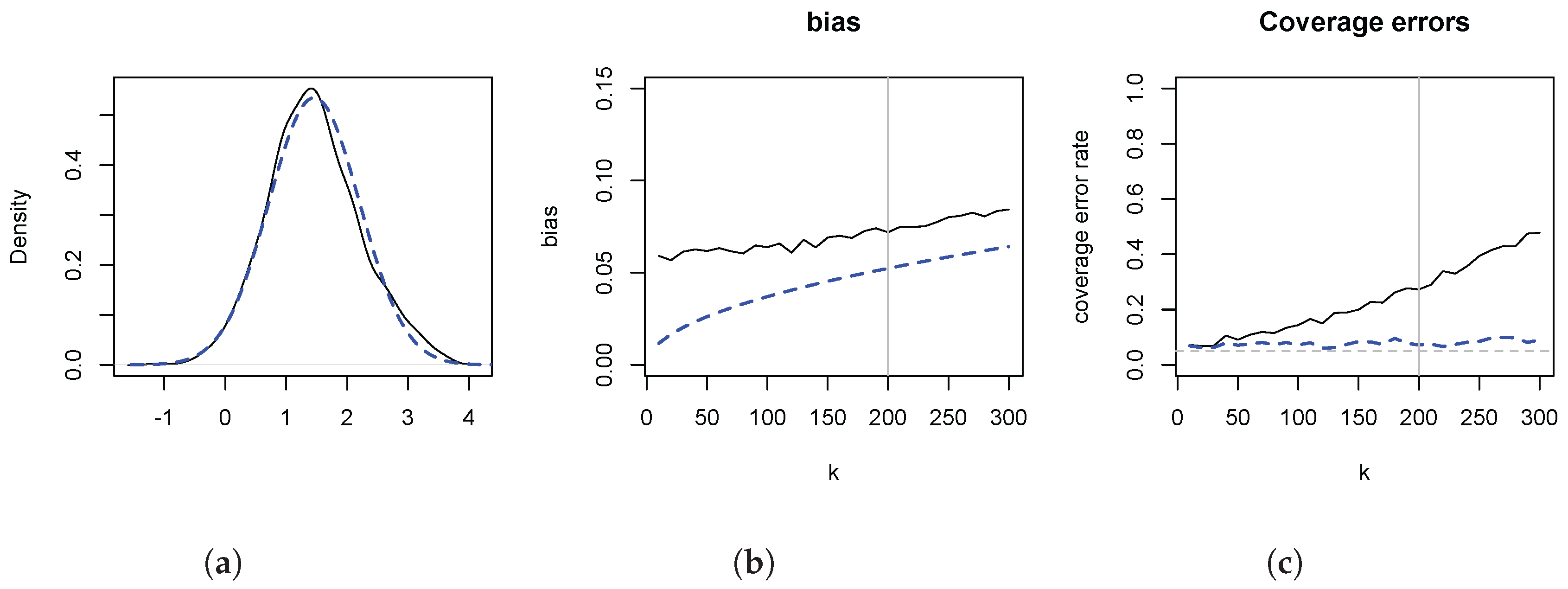
Figure 3 depicts the results. In panel (a) we illustrate the distributional theory, given by (8), for $k^{*}$, by plotting a kernel density estimate of $\sqrt{k^{*}}\widehat{\gamma }$ (solid line), as well as a normal density with variance $(5/4){\gamma }^2$, centered on the empirical mean of the simulated data. The two are in close agreement. The figure also implies that any inferential problems are due to location shifts. In panel (b) we contrast the empirical distortions (solid line) with $b_{k,n}$ (dashed line). $\widehat{\gamma }$ overestimates $\gamma$, and the distortion increases in k. It is evident that most of the distortion is captured by $b_{k,n}$. In panel (c) we illustrate the consequences of the distortions for statistical inference, by plotting the empirical coverage error rates of the usual 95% symmetric confidence intervals. The higher order distortions lead to undermining inference because of the considerable size distortions. For instance, at $k^{*}$, the empirical coverage error rate is 30% for a nominal 5% rate. Shifting the estimate by $b_{k^{*},n}$ reduces the coverage error rate to 7%.

Next, we consider the role of the sample size n. Reducing the sample sizes in the Monte Carlo to $n=1000$ yields results that are in line with the above theory, and therefore not depicted. The bias of $\widehat{\gamma }$ increases by a factor predicted by the theory, namely $b_{k,1000}/b_{k,\mathrm{10,000}}={10}^{1/2}=3.16$. The optimal $k^{*}$ shrinks by a factor of 4, as now $k^{*}=50$. The density of $\sqrt{k^{*}}\widehat{\gamma }$ is in good agreement with the theory, and empirical coverage error rates at this $k^{*}$ are 32% for the uncorrected and 11% for the corrected estimator. The empirical coverage error rate for the uncorrected estimator rises steeply after $k^{*}$, reaching 64% at $k=100$. Reducing the sample sizes further to 100 results in $k^{*}=20$, and an empirical coverage error rate for the uncorrected estimator of 46% at this $k^{*}$. Biases are increased by a factor $b_{k,100}/b_{k,\mathrm{10,000}}=10$.

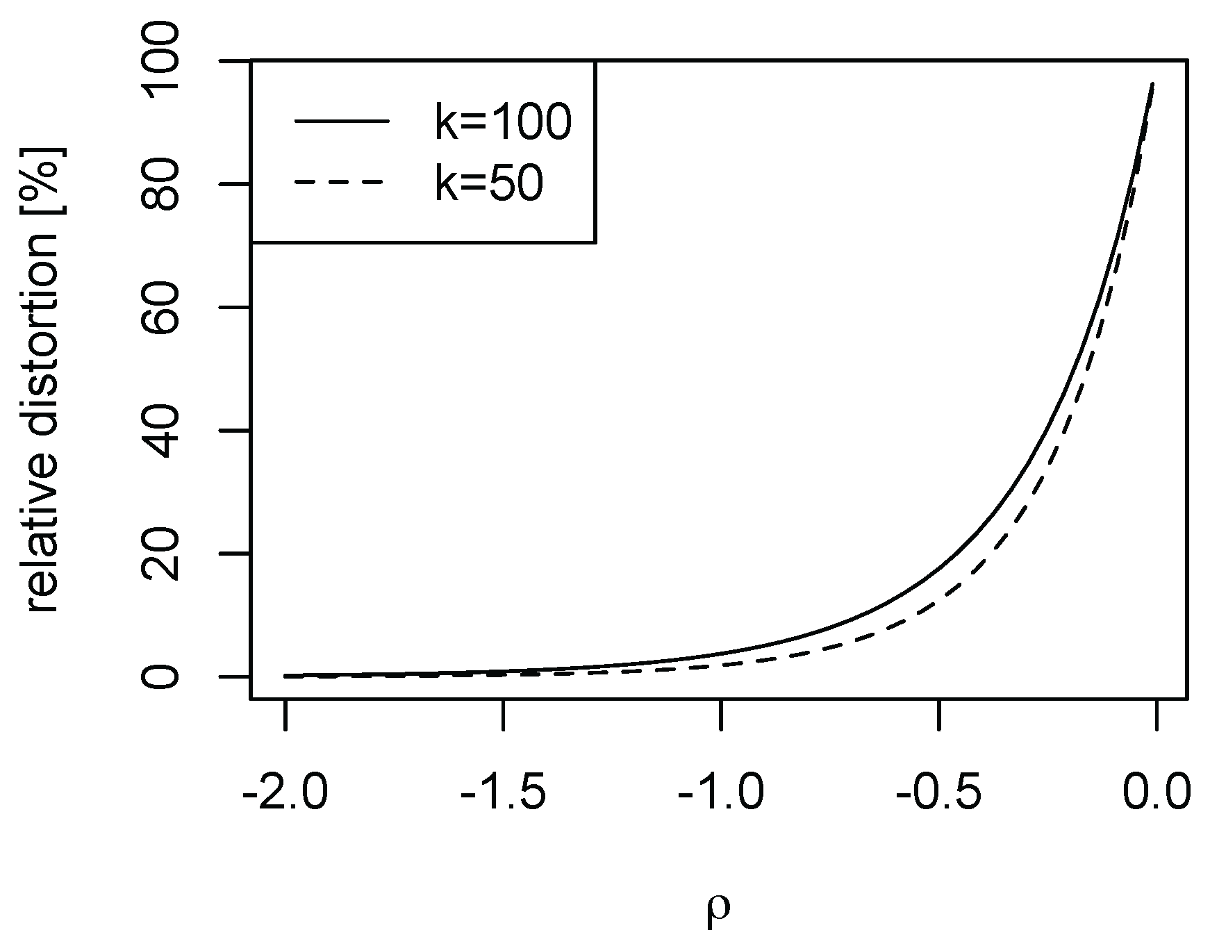
Finally, we illustrate the importance of the speed of decay in the nuisance function l of model (1). As $\rho$ falls in magnitude, the nuisance function l decays more slowly. For the Burr case with $\gamma =2/3$, we depict in Figure 4 $b_{k,n}$ as $\rho$ falls in magnitude for $n=1000$ and selected k. While for $\rho =-2$ the distortions are negligible (in line with Figure 2, it is evident that for small magnitudes of $\rho$ the higher order distortions cannot be ignored).

As the purpose of our simulation study is the provision of numerical evidence for our theory, we have used the theoretical bias function $b_{k,n}$ in the Burr case. When no such external knowledge is available, estimating the bias function requires non-parametric estimates of the second order parameter $\rho$ and the function $A(·)$. However, existing methods perform poorly, yielding excessively volatile estimates. The theory then informs a sensitivity analysis which is described in Section 4.1 in the context of our empirical application.

4. Empirical Illustration: Top incomes in the UK

Our empirical application uses administrative income tax return data are from the public-release files of the Survey of Personal Incomes (SPI) for the year 2009/10 (see e.g., Jenkins 2017 for a detailed description, and an analysis that includes rank size regressions). The SPI data underlie the UK top income share estimates in the World Top Incomes Database (WTID), and is a stratified sample of the universe of tax returns. The unit of taxation is the individual, and we use total taxable income as the income variable. The file contains 674,715 individuals, and we consider the n largest incomes.

In Figure 1 panel (a), we have depicted the Pareto QQ-plot for the 1000 largest incomes. It is evident that the data clearly reject a strict Pareto model: The plot exhibits a pronounced kink, and approximate linearity of the QQ plot only holds for the very highest upper order statistics. The function l in (1) captures this significant departure from the strict Pareto model. The Pareto QQ-plot thus conveys crucial information that is usually ignored by practitioners in economics, making it a key diagnostic device. For instance, a common mechanical approach is to set k by choosing ‘blindly’ (i.e., without reference to the Pareto QQ-plot) e.g., the top 1% or the top 1000 observations. Since the approximate linearity only obtains for about the 70 largest observations, the estimate of the slope parameter of the Pareto QQ-plot, i.e., the OLS estimator (3), will be severely biased if k is set to 1000 or higher. This is illustrated in panel (b) of the figure: The estimates fall for higher values of k, since the estimation procedure then attributes increasing weights to the left of the kink in the Pareto QQ-plot.

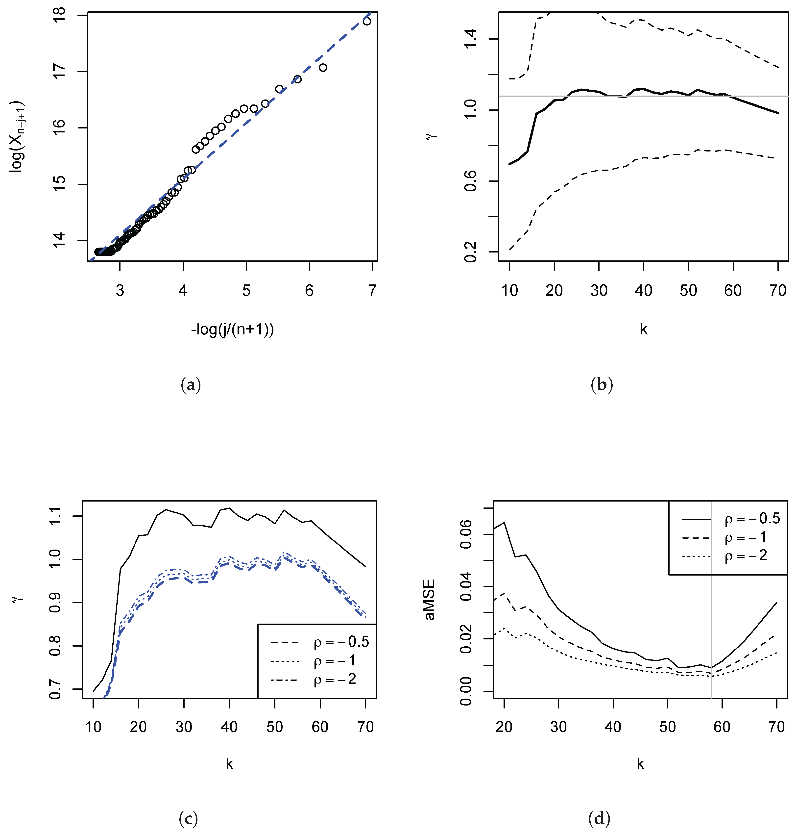
In the light of these observations, we restrict our subsequent analysis to the range of k in which the Pareto QQ-plot is approximately linear. We confirm this in Figure 5 panel (a), having restricted the plot to the $n=70$ highest incomes. The plot now appears fairly linear. In panel (b), we depict the regression estimates $\widehat{\gamma }$ and the 95% symmetric pointwise confidence intervals. One first visual way of choosing an estimate is to consider an area of the plot where the estimate is fairly stable (as is done by inspecting Hill or so-called alternative Hill plots) and picking the largest such k since the variance of the estimate falls in k. Such subjective choice would be around $k=60$ with an estimate of $\widehat{\gamma }=1.070$ (indicated by the horizontal faint line in the figure).4 Overall, the visual method would suggest an estimate of $\gamma$ between 0.9 and 1, implying very heavy tails. Taking into consideration the variability of the estimate, one cannot reject the hypothesis that the tail index be unity, i.e., Zipf’s law. Returning to panel (a) we have also plotted the line with slope 1. This line does well in describing the data. We turn to a method that permits an objective choice of a particular k, and examine the remaining distortions in the estimate of $\gamma$.

4.1. Sensitivity Analysis, and the Choice of k

The preceding analysis has shown that $\widehat{\gamma }$ is likely to suffer from positive higher order distortions, captured by $b_{k,n}$. Estimating this bias function requires non-parametric estimates of the second order parameter $\rho$ and the function $A(·)$, but existing methods perform poorly, yielding excessively volatile estimates. Hence we limit ourselves to a sensitivity analysis, taking $\rho$ as a sensitivity parameter, whose objective is to gauge plausible values of the potential distortions based on diagnostics of the rank size regression. This approach is sketched next.

Following Beirlant et al. (1996), we observe that the mean weighted theoretical squared deviation

$$\frac{1}{k}\sum _{j=1}^k{w}_{j,k}E{\left(\log \left(\frac{X_{n-j+1,n}}{X_{n-k,n}}\right)-\gamma \log \left(\frac{k+1}{j}\right)\right)}^2$$

equals, to first order,

$$c_{k}Var\left(\widehat{\gamma }\right)+d_k\left(\rho \right)b_{k,n}^2$$

(10)

for some coefficients $c_k$ depending only on k, and $d_k\left(\rho \right)$ depending on k and $\rho$ (these are stated explicitly in the Appendix A). Set $w_{j,k}\equiv 1$. An estimate of the mean theoretical deviation is the mean of the squared residuals $k^{-1}SS{R}_k$ of the rank size regression. In view of the usual bias-variance trade-off for our estimator $\widehat{\gamma }$ for fixed n, we ascribe all the measured deviation $k^{-1}SS{R}_k$ to the bias, thereby defining a very conservative bound, and let

$${\tilde{b}}_{k,n}\left(\rho \right)={[k^{-1}SS{R}_k/d_k\left(\rho \right)]}^{1/2}$$

This conservative sensitivity analysis then consists of examining $\widehat{\gamma }-{\tilde{b}}_{k,n}\left(\rho \right)$ for a range of values of $\rho$.

Figure 5 panel (c) reports the results of such a sensitivity analysis for k being restricted to the $n=70$ highest incomes. Since under this restriction the Pareto QQ-plot is approximately linear, we expect that the remaining distortions are fairly modest. This is borne out in the sensitivity plot, as the precise value of $\rho$ now plays only a minor role.

Should a researcher wish to choose a particular k by minimising an approximation to the AMSE, Equation (10) is the basis of the procedure proposed in Beirlant et al. (1996): Apply two weighting schemes $w_{j,k}^{\left(i\right)}$ ($i=1,2$), estimate the corresponding two mean weighted theoretical deviations using the residuals, and compute a linear combination thereof such that $Var\left(\widehat{\gamma }\right)+b_{k,n}^2$ obtains. We have carried out this programme (see Appendix A for further details) for weights $w_{j,k}^{\left(1\right)}\equiv 1$ and $w_{j,k}^{\left(2\right)}=j/(k+1)$ for given $\rho$, and Figure 5 panel (d) depicts the results. Minimising this approximation to the AMSE yields $k^{*}\left(\rho \right)$, which, for $\rho \in \{-2,-1,-0.5\}$, resulted in $k^{*}=58$ across the selected $\rho$, for which ${\widehat{\gamma }}_{k^{*}}=1.089$ obtains. In view of the results depicted in panel (c) it is not surprising that changing $\rho$ has only a small effect. This estimate of $\gamma$ is very close to the subjective visual choice of $\widehat{\gamma }$ of 1.075, reported above, based on Figure 5b.

5. Conclusions

The OLS estimator of the slope coefficient in the rank size regression (shifted or unshifted) can suffer significant higher order distortions that arise from the slow decay of the nuisance function l in the model $1-F\left(x\right)=x^{-\frac{1}{\gamma }}l\left(x\right)$ for $\gamma >0$. Modeling the tail as second order regular variation, we have shown that the estimator over-estimates the true value in models in which l converges to a constant at a polynomial rate (i.e., in the leading heavy-tailed distributions). Our numerical illustrations have shown that these distortions can be dramatic, leading to test size distortions in which actual error rates are multiples of nominal error rates. The empirical illustration based on the Pareto QQ-plot has revealed a further distortion, namely the presence of a pronounced kink. Figure 1 has revealed that using the common rule to choose 1% of the observation for tail estimation would lead to a severe under-estimation of how heavy the tail is.

The higher order distortions are functions of $A(·)$ and the second order regular variation parameter $\rho$. Since existing methods usually result in poor estimates of these, reliable bias corrections are not feasible. In view of this we have proposed a sensitivity analysis based on diagnostics from the rank size regression. When applied to our data on top incomes, we still cannot reject the hypothesis $\gamma$ be unity, a situation often described in several fields as Zipf’s law (e.g., Schluter and Trede 2017).

The simplicity of the regression estimator is undoubtedly the principal reason for its popularity among practitioners in economics. This paper has shown that in many situations the naive (i.e., ‘blind’) use of this estimator should be considered with care: Pareto QQ-plot, the sensitivity plot and the AMSE plot convey jointly important information about the behaviour of the estimator.

References

- Atkinson, Anthony Barnes. 2017. Pareto and the upper tail of the income distribution in the UK: 1799 to the present. Economica 84: 129–56. [Google Scholar]
- Beirlant, Jan, Petra Vynckier, and Jozef L. Teugels. 1996. Tail index estimation, Pareto quantile plots, and regression diagnostics. Journal of the American Statistical Association 9: 1659–67. [Google Scholar]
- Beirlant, Jan, Yuri Goegebeur, Johan Segers, and Jozef L. Teugels. 2004. Statistics of Extremes. Wiley Series in Probability and Statistics; Chichester: Wiley. [Google Scholar]
- Burkhauser, Richard V., Shuaiz hang Feng, Stephen Jenkins, and Jeff Larrimore. 2012. Recent trends in top income shares in the USA: Reconciling estimates from March CPS and IRS tax return data. Review of Economics and Statistics 94: 371–88. [Google Scholar]
- Cowell, Frank A. 1989. Sampling variances and decomposable inequality measures. Journal of Econometrics 42: 27–41. [Google Scholar]
- Cowell, Frank A., and Emmanuel Flachaire. 2007. Income distribution and inequality measurement: The problem of extreme values. Journal of Econometrics 141: 1044–72. [Google Scholar]
- Csorgo, Sandor, Paul Deheuvels, and David Mason. 1985. Kernel Estimates of the Tail Index of a Distribution. The Annals of Statistics 13: 1050–77. [Google Scholar]
- Davidson, Russell, and Emmanuel Flachaire. 2007. Asymptotic and bootstrap inference for inequality and poverty measures. Journal of Econometrics 141: 141–66. [Google Scholar]
- De Haan, Laurens, and Ana Ferreira. 2006. Extreme Value Theory. New York: Springer. [Google Scholar]
- De Haan, Laurens, and Ulrich Stadtmüller. 1996. Generalized regular variation of second order. Journal of the Australian Mathematical Society (Series A) 61: 381–95. [Google Scholar]
- Dekkers, Arnold L. M., John H. J. Einmahl, and Laurens de Haan. 1989. A moment estimator for the index of an extreme-value distribution. Annals of Statistics 17: 1833–55. [Google Scholar]
- Embrechts, Paul, Claudia Kluppelberg, and Thomas Mikosch. 1997. Modelling Extremal Events. Berlin: Springer. [Google Scholar]
- Gabaix, Xavier, and Rustam Ibragimov. 2011. Rank - 1/2: A simple way to improve the OLS estimation of tail exponents. Journal of Business and Economic Statistics 29: 24–39. [Google Scholar]
- Hall, Peter. 1982. On some simple estimate of an exponent of regular variation. Journal of the Royal Statistical Society Ser. B 44: 37–42. [Google Scholar]
- Kratz, Marie, and Sidney I. Resnick. 1996. The QQ-estimator and heavy tails. Communications in Statistics. Stochastic Models 12: 699–724. [Google Scholar]
- Jenkins, Stephen P. 2017. Pareto models, top incomes and recent trends in UK income inequality. Economica 84: 261–89. [Google Scholar]
- Schluter, Christian, and Mark Trede. 2002. Tails of Lorenz curves. Journal of Econometrics 109: 151–66. [Google Scholar]
- Schluter, Christian, and Mark Trede. 2017. Size distributions reconsidered. Econometric Reviews. forthcoming. [Google Scholar]
- Schultze, J., and J. Steinebach. 1996. On least squares estimates of an exponential tail coefficient. Statistics and Decisions 14: 353–72. [Google Scholar]
- Wellner, Jon A. 1978. Limit theorems for the ratio of the empirical distribution function to the true distribution function. Zeitschrift fuer Wahrscheinlichkeitstheorie und verwandte Gebiete 45: 73–88. [Google Scholar]