Estimating Unobservable Inflation Expectations in the New Keynesian Phillips Curve


Department of Economics, University of Ottawa, 120 University Private, Ottawa, ON K1N 6N5, Canada
†
I would like to thank the participants to the brown bag workshop at the University of Ottawa for their comments and suggestions. I am also grateful to two anonymous reviewers for their constructive comments, which helped improve the quality of the paper. The usual disclaimer applies.
Econometrics 2018, 6(1), 6; https://doi.org/10.3390/econometrics6010006
Submission received: 1 December 2017
/
Revised: 27 January 2018
/
Accepted: 31 January 2018
/
Published: 5 February 2018
(This article belongs to the Special Issue Recent Developments in Macro-Econometric Modeling: Theory and Applications)
Abstract
:This paper uses an econometric model and Bayesian estimation to reverse engineer the path of inflation expectations implied by the New Keynesian Phillips Curve and the data. The estimated expectations roughly track the patterns of a number of common measures of expected inflation available from surveys or computed from financial data. In particular, they exhibit the strongest correlation with the inflation forecasts of the respondents in the University of Michigan Survey of Consumers. The estimated model also shows evidence of the anchoring of long run inflation expectations to a value that is in the range of the target inflation rate.
JEL Classification:
C1; E3; E51. Introduction
Expectations about future values of inflation and other economic variables play a central role in macroeconomic models. Theoretical research can provide precise information about the type of expectations that should affect the economy (of firms, households, policymakers, etc.) and specify the way in which these expectations should be formed (from rational expectations to alternative forms of bounded rationality). However, expectations cannot be directly observed from the data, which implies that the recommendations of the theoretical model are often difficult to translate into empirical research. It is then not surprising that the question of how to measure expectations has been at the center of a long stream of research in empirical macroeconomics. One branch of this literature, which builds upon the original work of McCallum (1976), has focused on the development of econometric-based measures that can be employed to approximate expectations in the models to be estimated. Another approach, which has become increasingly common in recent years, is to use survey data, or other measures that can be extracted from the observable data, as a proxy for expectations.
This paper is related to the literature concerned with the measurement of expectations in models of the New Keynesian Phillips Curve (NKPC). In particular, this work contributes to the branch of research that examines the extent to which observable measures of expectations are able to approximate their model-consistent counterparts (see, among the others, Roberts 1995; Nunes 2010; Coibion and Gorodnichenko 2015; Coibion et al. 2017; Lopez-Perez 2017). The paper follows along the lines of this literature, and in particular it builds upon Coibion and Gorodnichenko (2015). As in these previous contributions, I take the NKPC model and its predicaments seriously. However, I use a very different methodological approach. Most of the works in this area are focused on the analysis of the model fit to the data when alternative proxies for expectations are used in the estimation. Instead, I employ an econometric framework and Bayesian methods to reverse engineer the path of inflation expectations implied by the NKPC and the data. I then compare this path to several available measures of inflation expectations. The questions of interest in this paper are: 1. In the context of a NKPC model, what path of expectations emerges from the data? And, in more detail, what does this path look like? What are its time series properties? 2. Is this path similar to the expectations that we can observe from surveys or compute from the data?
This paper is not the first one to treat expectations as unobservable variables and to estimate their path using an empirical framework and the data. Previous contributions have adopted this approach to study trend inflation and long run inflation expectations (see, in particular, Kozicki and Tinsley 2012; Chan et al. 2015; and Stock and Watson 2016), using frameworks that are built upon the econometric model of Stock and Watson (2007). The strategy employed by some of the contributions in this area is to exploit survey data on expectations to back-up estimates of the parameters of the model (as for instance in Nason and Smith 2013; Mertens 2016; Mertens and Nason 2017). The empirical model of expectations used in this paper is less general than the frameworks adopted in this literature, and it is dependent on the equation of the NKPC. However, the model is estimated using a more unrestricted approach, in which the path of expectations is obtained jointly with all the other parameters of the model. The framework employed in this paper is closer to Blanchard (2016). However, Blanchard (2016) uses the model to study the changes over time in the parameters of the Phillips Curve, while I am most interested in estimating the unobservable expectations and in computing their correlation with the available data on inflation forecasts. Methodologically, the Bayesian procedure adopted in this work follows the approach used by Primiceri (2006) to estimate the unknown natural rate of unemployment.
The results show that the estimated expectations are relatively persistent, and that they are not characterized by permanent shifts over time. The estimated path resembles the data from various surveys, especially in some parts of the sample. In particular, the paper finds that household expectations are strongly correlated with the model-consistent expectations that emerge from the NKPC. This result confirms the conclusions of Coibion and Gorodnichenko (2015). The estimated slope of the Phillips curve, and its changes over time, are also in line with the values obtained in the previous literature (Coibion and Gorodnichenko 2015; Blanchard 2016). Finally, I find evidence of the anchoring of long run inflation expectations to a value that is in the range of the target inflation rate, which is consistent with the conclusions of Bernanke (2010) and Svensson (2015).
It is worth remarking that the analysis performed in this paper is not normative, in the sense that the econometric model used to estimate expectations does not make any structural assumptions about the way in which expectations are formed. This implies that the results of this study cannot be directly employed for monetary policy analysis, because the framework that I adopt cannot make any statements about how expectations would change following a change in policy. However, the results of this paper, in particular those related to the relationship between the estimated expectations and the available survey data, are relevant, and can be exploited, in the research using the NKPC for normative monetary policy analysis.
The remainder of the paper is organized as follows. Section 2 describes the model and Section 3 outlines the empirical strategy used to estimate its parameters and the unknown inflation expectations. Section 3 discusses the results and compares the estimated path of expectations to the available data on inflation forecasts. Section 4 concludes. The Appendix A provides more details about the Bayesian empirical procedure and its implementation.
2. The Model
The model is a standard expectations-adjusted New Keynesian Phillips Curve (NKPC), the specification that I employ is the same as in Coibion and Gorodnichenko (2015) and Svensson (2015):
In this equation, is the inflation rate, is expected inflation, is a measure of “slack”, such as the unemployment or output gap1, and is a shock.
The basic NKPC is augmented of an empirical model for expectations:
where and are and innovations, respectively. I assume that and Frameworks similar to the one described by (2) and (3) have been previously employed in the literature to characterize the path of inflation expectations (for instance by Blanchard 2016) but also other unobservable variables, as the natural rate of unemployment (Staiger et al. 2001; Primiceri 2006).
The econometric model for defined by (2) and (3) is relatively simple, but flexible enough to be able to reproduce several of the features that could potentially be present in the time series path of this variable. More specifically, the parameter can measure the autocorrelation of inflation expectations over time, the innovation can capture transitory variations in expectations, while permanent shifts can be reflected by changes in the time-varying intercept . The intercept can be viewed as related to the expected long run inflation rate according to the relationship: . Thus, variations in can further be interpreted as revisions in agents’ long run inflation expectations.2
The path of is estimated jointly with the parameters of the econometric model defined by (2) and (3), the history of , and the parameters of the NKPC (1), using the observable data for and Thus, the time series of inflation expectations emerging from this estimation procedure will reflect the information carried by the data, “filtered” through the structure of the NKPC.
3. Estimation
The model is estimated using data for the U.S. The inflation rate is the annualized log difference in the quarterly CPI (Consumer Price Index). The measure of “slack” is the unemployment rate gap , where is the civilian unemployment rate while is the CBO measure of the short-term NAIRU.3 The choice of the variables to be used in the estimation follows Coibion and Gorodnichenko (2015), and allows the results to be comparable; however, robustness checks performed replacing the CPI with core or headline PCE (Personal Consumption Expenditure) delivered comparable results. The data are quarterly and go from to .4 The main analysis uses observations from to while data from to are used to set the parameters of the prior distributions in the Bayesian estimation procedure.
As previously explained, in the second part of the analysis I compare the estimated path of to observable data on inflation forecasts. Following Coibion and Gorodnichenko (2015), I use three different sources of data, with the purpose of capturing the expectations of different groups of agents in the economy. The first source is the University of Michigan Survey of Consumers, which measures households’ inflation expectations. The data that I employ for the baseline analysis are the “median forecast of price changes over the next 12 months”, available from the University of Michigan Surveys of Consumers webpage. The series is monthly and was transformed to quarterly observations for the period .5 The second source of data reflects the market’s inflation expectations. The specific measure that I employ is maintained by the Federal Reserve Bank of Cleveland, which uses “Treasury yields, inflation data, inflation swaps, and survey-based measures of inflation expectations to calculate the expected inflation rate (CPI)”.6 The series includes monthly data starting from January 1982, which were transformed to quarterly observations from to . The last source of data that I employ is the Survey of Professional Forecasters. The inflation forecasts contained in this survey are widely used to approximate expectations in empirical macroeconomic research. The specific series that I use are the median of the respondents’ forecasts of headline and core CPI inflation for the current period, the next period, and the next year (i.e. the average of the next four quarters). The data are quarterly; for headline CPI the sample starts in , while for core CPI the data are only available from .
3.1. Empirical Strategy
Using a framework with time-varying parameters, Blanchard (2016) shows that the slope of the NKPC decreased after 1985, a result that is supported by the estimations of Coibion and Gorodnichenko (2015). In order to account for this result, I follow the approach adopted by Coibion and Gorodnichenko (2015) and I estimate a modified version of the NKPC:
where is an indicator variable that takes the value of 1 for .7 The parameter captures the possible shift in the slope of the NKPC that happened in the mid-1980s.
The framework composed of Equations (4), (2), and (3) is estimated using Bayesian methods. The measure of interest is the joint posterior distribution of all the parameters of the model, together with the histories of the time-varying intercept and expectations . The estimation is performed through a Markov Chain Monte Carlo (MCMC) procedure which uses the data and the (known) conditional distributions of the parameters and variables of interest to obtain draws from their (unknown) joint posterior.
The empirical model to be estimated can be written in vectorial form as:
where , , and , with Notice that S is a matrix with zeros everywhere, except for the element in the first row, first column, which is equal to . Using this notation, the assumptions on the prior distributions of the parameters and variables of interest can be written as follows:
where denotes the Inverse Wishart distribution with scale parameter S and v degrees of freedom.
The assumptions about the priors follow previous works that use Bayesian methods to estimate models similar to (5)–(7), in particular Primiceri (2006). The vector B of (time invariant) parameters of the NKPC is assumed to have a Normal prior distribution. The priors for the initial state of the vector , denoted by , and the initial value of expectations, denoted by , are also assumed to be normally distributed. These assumptions are standard in the literature. For the vector B, the Normal prior and the Gaussian conditional likelihood of the data implied by (5) give a conditional posterior that is also a Normal distribution, with parameters that can be computed using simple formulas. For the vector and expectations , the priors (9) and (10), together with the laws of motion given by (5)–(7) and the assumptions about the distributions of the shocks of the model, imply that the conditional posteriors of and are known. Further details about these distributions are provided in the Appendix A. With respect to the variances of the shocks, the assumptions on their distribution are restricted by the fact that variances need to be non-negative numbers. The standard choice in the literature is to use an Inverse Wishart distribution, which is defined on positive-definite matrices. In Bayesian estimation, this assumption is convenient also because it allows to exploit the properties of conjugate priors. In the specific framework under analysis, the variances , , and , are assumed to be independent of each other and to have each an Inverse Wishart prior as defined by (11)–(13).8 The corresponding conditional posterior probabilities are detailed in the Appendix A.
The parameters of the prior distributions (8)–(13) are set using the training sample . Within this period, I approximate expectations as . I employ the approximated expectations, together with the observations for and to estimate Equations (5) and (6) by OLS, using a time-invariant intercept in the equation for inflation expectations. I then exploit the results of these regressions to set the parameters of the prior distributions. In the Normal prior (8), is the estimated vector of parameters B obtained from (5) and is the variance of this estimate. Similarly, in the Normal prior (9), is the estimated vector of parameters D obtained from (6) and is the variance of this estimate. In (10), denotes expected inflation at time 0 of the estimation period, i.e. in . In the Normal prior for this variable, the mean is the approximated value of expectations for the last period of the training sample, and is the variance of in the training sample. In the Inverse Wishart priors for and , the parameters and are the variance of the residuals in the OLS regressions of Equation (5) and (6), respectively. In both (11) and (12), is the number of observations in the training sample. Finally, is the variance of the OLS estimate of the time-invariant intercept in (6). In the prior for , the scale parameter is multiplied by the factor and the degrees of freedom are set to 2, which corresponds to the dimension of plus one. The assumptions on the prior for follow Cogley and Sargent (2001) and Primiceri (2005); they are adopted to avoid an excessive time-variation of and to ensure, at the same time, that this time variation is driven by the data and not by the choice of parameters in (13). The results are almost unaffected if alternative values of (for instance, 0.1 or 0.5) are used instead.
The conditional posteriors of the parameters and variables of interest can be obtained from the prior distributions, using the likelihood of the data and the properties of conjugate priors. These posteriors are then employed in the MCMC algorithm to produce draws from the unknown joint posterior distribution of the parameters , , , , , , and histories and . The MCMC method is a simulation procedure used to generate draws from unknown (or complex) joint posterior distributions. The algorithm samples successively from known distributions, which in the framework under study in this paper are the conditional posteriors of the parameters of the model and histories and . The “ chain” structure of the procedure implies that each new set of values is drawn conditional on the values obtained in the previous step of the sequence. Once the algorithm has converged, the additional draws will have the same distribution as if they were sampled from the true joint posterior of interest.
In the model described by (4), (2), and (3), the MCMC procedure is implemented according to the following sequence. First, a history is drawn conditional on and the parameters and . A value for can then be sampled given . Second, a history is drawn conditional on , the parameters B, , and , and the data. A value for can then be sampled given , , and . Finally, values for B and can be drawn conditional on and the observed data. The first 200,000 draws are discarded as burn in period, then one every 300 draws is saved until a total of 1000 is retained. The Appendix A provides a detailed description of the MCMC procedure and its implementation.
4. Results
The MCMC algorithm outlined in the previous section delivers 1000 draws from the joint posterior distribution of the parameters , , , , , , and histories and . These values are used to produce the results discussed in this section. The algorithm converges quickly and is quite insensitive to changes in the assumptions about the parameters of the prior distributions.9 The plots of the retained draws do not exhibit evident autocorrelation patterns and, overall, the procedure seems to perform well given the framework and the data at hand. Some convergence diagnostics are presented in the Appendix A.
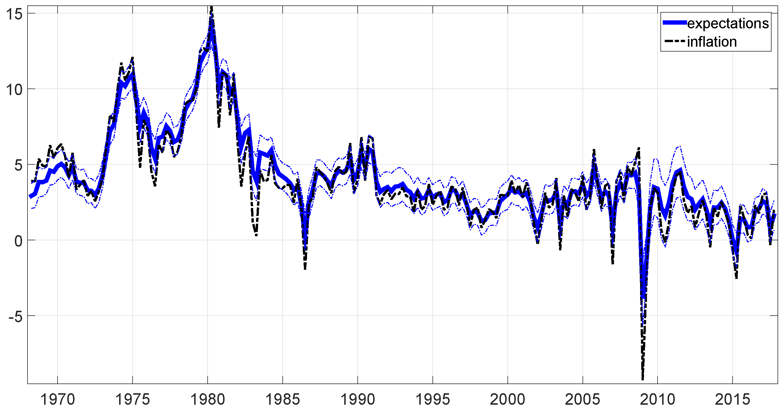
The estimated path of inflation expectations is reported in Figure 1. This figure shows the median value of the retained draws of for each time the dotted bands are the 16th and 84th percentiles of the draws. The figure also reports the path of the inflation rate for comparison. Figure 2 provides some further information by plotting the difference between the actual inflation rate and the median of the draws of . These figures show that the estimated expectations quite closely track the behaviour of the actual inflation rate, but their changes over time are smoother. Expectations mistakes are larger in more turbulent times, as for instance in the 1970s or during the recent financial crisis. Overall, the estimated expectations seem to exhibit a behaviour that is consistent with what we would have anticipated, and that is relatively easy to rationalize.
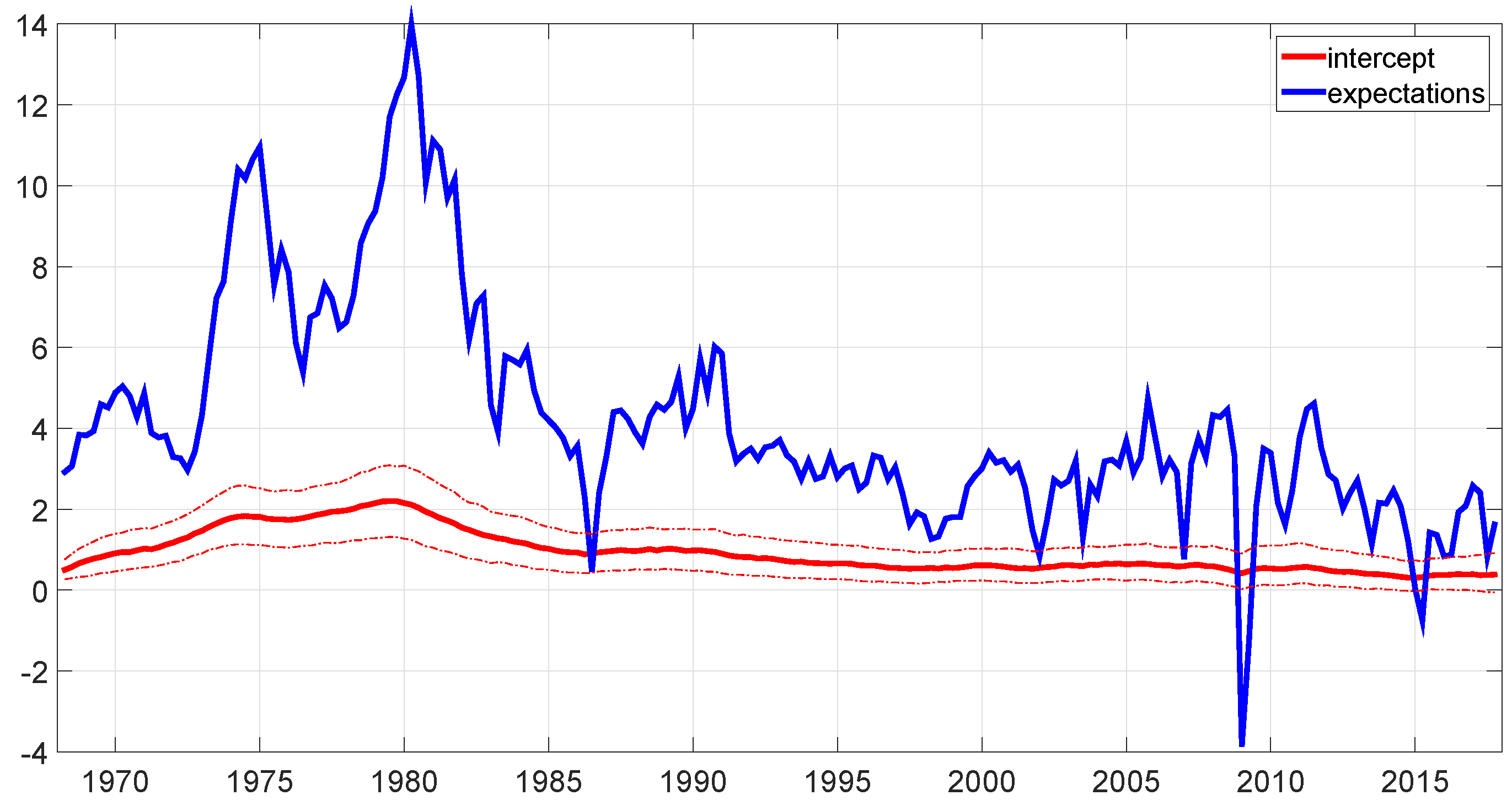
Figure 3 analyses the estimated history of inflation expectations and its components in more detail. More specifically, the figure reports the median value of the retained draws of for each time the dotted bands are the 16th and 84th percentiles of the draws. The figure also shows the median path of It is clear from this figure that the contribution of the time-varying intercept to the pattern of expectations is quite moderate. The estimated expectations do not seem to feature any sizeable permanent changes during the time period under analysis, and starting from the mid 1980s, the median value of stabilizes around values in the range 0.4–0.6.
The estimated parameters of the model are reported in Table 1. This information can be used to study the time-series properties of The median value of (0.7606) indicates that inflation expectations are quite autocorrelated over time. As predictable given the path of shown in Figure 3, the volatility of the permanent shocks is very small (0.0273). The transitory shocks have much larger volatility, and because of the autocorrelation implied by the magnitude of , they are predicted to have long lasting effects on the path of
The slope of the Phillips curve (i.e. the parameter ) reported in Table 1 is in the range of values obtained in recent works using similar models of the NKPC (Blanchard et al. 2015; Coibion and Gorodnichenko 2015; Svensson 2015; Blanchard 2016). The estimates point in the direction of a shift in the slope of the Phillips Curve in the mid-1980s, although the parameter is not statistically significant. The results are consistent in magnitude with the time-varying slope estimated by Blanchard et al. (2015) and Blanchard (2016), and with the values of both and obtained by Coibion and Gorodnichenko (2015).10
Finally, the value of and the path of can be used to study the behaviour of long run inflation expectations based on the interpretation of the time-varying intercept as The value of computed using this relationships has been in the range 1.5%–2.5% since the late 1990s. Thus, the estimated model does seem to suggest that long run inflation expectations have been “anchored” to the target rate for quite a few years. This result is again consistent with the conclusions of Blanchard (2016).
4.1. Comparison with the Observable Data on Expectations
Next, I study the extent to which the estimated path of is comparable to the available inflation forecasts data series described in Section 3. Figure 4 and Figure 5 report the median, and 16th and 84th percentiles, of the retained draws of together with the Michigan, Cleveland, and SPF measures of inflation expectations. For the SPF, I report the inflation forecasts for the next quarter (denoted as ) and for the next year (denoted as y). Figure 4 shows all the available data, while Figure 5 focuses on the sub-sample , which is the period under analysis in Coibion and Gorodnichenko (2015).
Table 2 and Table 3 report information about the correlations between the estimated path of and the observable measures of inflation expectations. For each measure, one correlation value is computed with each of the 1000 retained draws of ; the tables report the median, 16th and 84th percentiles of these values. Table 2 uses all the available data, while Table 3 splits the sample in two periods: before (excluded) and after (included). Again, the analysis on the split sample is done to compare the results with those of Coibion and Gorodnichenko (2015). In this table, the data from the SPF includes one additional variable, inflation forecasts for the current period, for both headline and core CPI. 11
Figure 4 and Figure 5 show that, in most periods, the estimated path of mimics the behaviour of several of the available measures of inflation forecasts. These results are confirmed by the correlations reported in Table 2 and Table 3. Most notably, the forecasts of the University of Michigan Survey of Consumers are found to be very highly correlated with the estimated expectation, particularly in the part of the sample before 2007 (the median correlation is 0.9128 for this period). In addition, Figure 5 shows that the forecasts of the Michigan Survey still behave quite similarly to the estimated in the years from 2007 to 2012 (result that is consistent with the findings of Coibion and Gorodnichenko 2015), but the relationship seems to become weaker after 2012. In general, Table 3 suggests that for several of the measures the correlation with the estimated decreases after 2007, with the exception of the expectations computed by the Federal Reserve Bank of Cleveland and the SPF forecasts of headline CPI inflation for the current period.
The findings of this paper contribute to the discussion about the “missing disinflation” puzzle, which is the focus of the analysis of Coibion and Gorodnichenko (2015). This puzzle refers to the absence of disinflation during the recent Great Recession, when the “slack” in the economy was very high so, according to standard models of the Phillips curve, the inflation rate should have been much lower. A model of the Phillips Curve as the one described by (1) will rationalize the variation in as due to changes in the measure of slack , to realizations of the shocks , and to the behaviour of expectations. The specific framework employed in this paper allocates this variation among , , and , by estimating the parameters of the models jointly with the entire history . This implies that, by construction, any missing disinflation (or excess inflation) arising from the estimated model will be accompanied by a path that can rationalize it. The exercise of comparing the observable measures of expectations to the estimated history can thus also provide information on the extent to which each of these measures can explain the missing disinflation. As shown in Figure 5, in the years from 2007 to 2012 the inflation forecasts of the Michigan Survey appear to more closely track the behaviour of the estimated expectations relative to the Cleveland or SPF forecasts. This result suggests that, indeed, the expectations of households recorded in the Michigan Survey can explain the missing disinflation puzzle, consistently with what argued by Coibion and Gorodnichenko (2015) and Binder (2015).
To provide a more thorough analysis of the similarities between the estimated and the observable inflation forecasts, I computed a few other statistics in addition to the correlations reported in Table 2 and Table 3. These statistics are the average, variance, and first order autocorrelation of the expected inflation series. The results obtained using all the available data are shown in Table 4, while Table 5 and Table 6 focus on 3 different sub-periods: the period before the Great Moderation (1978–1984), the Great Moderation (1985–2006), the Great Recession and post-Great Recession period (2007–2017).12 For simplicity of the analysis, in this exercise I only used the median of the retained draws of .
Table 4 and Table 5 show that the estimated expectations and the observable inflation forecasts imply very similar average expected inflation rates, although the differences are slightly larger for the period 2007–2017 (see Table 5, third column). In terms of variances, Table 4 suggests that the estimated series is generally more volatile than the observable measures of expectations. However, the results reported in Table 6 indicate that there are some differences across measures and across periods. For instance, the expectations recorded in the Michigan Survey exhibit a volatility that is quite high, and almost comparable to that of , in the sub-sample 1978–1984 but not in later years. On the other hand, the SPF forecasts of headline CPI inflation for the current period are as volatile as the estimated expectations across the entire sample period. The variance of all the other observable measures of expectations is lower, particularly in the years from 2007 to 2017. Finally, Table 4 and Table 7 report the first order autocorrelations of the series. The Michigan Survey data and the estimated expectations exhibit very similar autocorrelations; this is true across the entire sample period under analysis. With respect to the other measures, many of them (specifically, the SPF inflation forecasts for the next period or the next year and the Cleveland inflation expectations) seem to be more autocorrelated than the estimated , especially during the sub-period 1985–2006.
Theoretical models of the NKPC are typically clear about what type of expectations should be included in equations like (1). For instance, in the standard New Keynesian model presented in Gali (2008), expectations are assumed to be formed at time t for the horizon . As these models are often interpreted in terms of quarterly data, the horizon for which they assume expectations to be formed is in fact very short. The framework that I employ in this paper, however, is built to simply reverse-engineer a path of the variable , that evolves according to (2), and that captures the fraction of the variation of that cannot be explained by or attributed to the shock This implies that the estimated path of could, in practice, reflect different types of expectations. Overall, the results presented so far seem to indicate that the short term measures of expectations employed in the analysis resemble the estimated path of model-consistent expectations in several directions. However, longer term expectations could in principle perform equally well.
In order to address this question, I considered one additional observable measure of expectations: the Michigan Survey “median forecast of price changes over the next 5 to 10 years”. I examined the correlation with the estimated , in addition to the variance and the autocorrelation of the series, and I compared these statistics to those obtained in the first part of the analysis for the Michigan Survey “median forecast of price changes over the next 12 months”. As the forecasts over the next 5 to 10 years are only available starting from 1990, I computed all the statistics for the full sample 1990–2017, and for the two sub-samples 1990–2006 and 2007–2017. The results of this exercise are reported in Table 8. The table shows that for almost all the calculated statistics, the estimated path of expectations is more similar to the forecasts of inflation over the next 12 months than to the forecasts over the next 5 to 10 years. This result seems to indicate that the estimated history more closely mirrors expectations for the short horizon, in line with the theoretical assumptions of the NKPC model. However, the differences emerging from Table 8 are not very large, and do not allow to make strong statements in this respect.
The path of estimated in this paper could capture different types of expectations not only with respect to the horizon of reference, but also in other dimensions. For instance, these expectations could refer to alternative measures of inflation, or they could reflect the forecasts of some groups of the population more than others. In terms of inflation measures, the SPF data used in the paper include both headline and core CPI inflation forecasts. This choice was an attempt to account for the fact that agents could base their expectations over different measures of inflation. Unfortunately, the core inflation forecasts are only available for a very short period of time, so the results of this analysis are only indicative. With respect to the expectations of different demographic groups, the recent work of Binder (2015) has shown that their impact on the dynamics of inflation might not be uniform.13 To explore this direction in more depth, I performed one last exercise in which I studied the correlations between the estimated expectations and the Michigan Survey “median forecast of price changes over the next 12 months” for different demographic groups. In this exercise, I used all the available disaggregated data, for all the available years. The results are reported in Table 9; the first row reproduces the results obtained from the aggregate data, for comparison. The table shows that the correlation between the estimated expectations and the survey data is roughly the same across regions, and is not affected by the gender of the respondents. The forecasts of respondents over 55 years of age or in the bottom 33% income group are less correlated to the estimated and, in general, the correlations increase with the income and education of the respondents. These results are consistent with those reported by Binder (2015), although, overall, the differences among demographic groups emerging from Table 9 do not seem to be very large.
As previously mentioned, I performed several robustness checks using different values of the parameters in the prior distributions (more specifically, the means and variances of the normal distributions and the scale parameters of the Inverse Wishart distributions). I also experimented with different burn in periods and sampling lengths in the MCMC estimation procedure, as detailed in the Appendix A. Finally, I repeated the estimation using core or headline PCE instead of CPI to compute . The main results of the paper were materially unaffected by these changes.
5. Conclusions
This paper employed an econometric model to estimate the model-consistent path of inflation expectations emerging from the NKPC and the data. The estimated expectations are relatively persistent and do not exhibit large permanent shifts during the period under analysis, not even following major events as for instance the recent financial crisis. These results can be interpreted as providing evidence of the anchoring of long run inflation expectation to the target rate.
The path of expectations estimated in this paper shows the strongest correlation with the inflation forecasts of households recorded in the University of Michigan Survey of Consumers. This is true especially for the period before 2012. This result strongly supports the argument of Coibion and Gorodnichenko (2015), who suggest that households forecasts are the most model-appropriate measure of expectations in the context of the NKPC, as they are close to the expectations of firms which are not observable in the data.
Clearly, the results of this paper are model dependent, as the MCMC procedure used to estimate the path of expectations exploits the equation of the NKPC. In addition, this work does not make any structural assumptions about the way in which expectations are formed, and how they would change following a change in policy. In this sense, the analysis is fully positive, and does not aim at making statements about policy recommendations. Despite these caveats, I do believe that the results of this paper are important for the literature on monetary policy analysis in the context of the NKPC. In particular, the conclusions of this paper are in line with the recommendations of Coibion and Gorodnichenko (2015) and Coibion et al. (2017) about the use of survey data, in particular household inflation forecasts, as a proxy for expectations in monetary policy analysis.
Conflicts of Interest
The author declares no conflict of interest.
Appendix A. The Markov Chain Monte Carlo Procedure
The measure of interest is the joint posterior distribution of all the parameters of the model, together with the histories of the time-varying intercept and the history of expectations . In order to simplify notation, I am going to group the parameters as and ; the superscript T denotes the history of the variable up to time T. Using this notation, the posterior distribution of interest can be written as:
where is the observable data. As previously explained, the MCMC procedure samples from the conditional posterior distributions of the parameters of interest, which are known.
Drawing , and
I first draw a path for the time varying intercept and a value of the parameters and The conditional distribution can be factored as shown in Carter and Kohn (1994):
where:
This expression can be used to draw a history . The values and can be obtained from the “Kalman smoother” of Carter and Kohn (1994). The smoother is based upon a forward recursion (the Kalman filter) that delivers the final values and , and on a subsequent backward recursions that gives each and 14 The formulas of the forward recursion, applied to the specific model under analysis in this paper, are:
The initial values of the recursion, and are set using data from the training sample, as discussed in the main text.
The final values of the recursion, and can be used to draw a value for from Then, this value can be used in the first step of the backward recursion to obtain and , and then these values can be used to draw a value for from The process can be repeated for all t. The generic formulas of this backward recursion are:
Notice that, because of the form of the matrix S, this approach will deliver vectors which are composed of a time-varying and a time-invariant (i.e. the value of will be the same for all t), consistently with the model described by (2) and (3).
Drawing a Path of Inflation Expectations
Given the history , the data, and the parameters of the NKPC, the conditional distribution of can be written as: . This density can be factored again following Carter and Kohn (1994) as:
The procedure for drawing is exactly the same as the one used for Notice that the equation of the NKPC can be re-arranged as: Given the data and the parameters in the left hand side of this equation is known. The formulas of the forward recursion used to obtain and are:
The initial values of the recursion, and are again set using data from the training sample, as explained in Section 3.1. The values and can be used to draw a value for from this value can be employed to obtain and , which can then be used to draw a value for from and so on. The formulas of the backward recursion are:
Drawing and
Given the assumption on the prior distributions, the conditional posteriors of the variances and (the only non-zero element of the matrix S) are Inverse Wishart distributions:
where:
- Values of and can be sampled from these Inverse Wishart distributions.
Drawing the Parameters of the NKPC
Given the assumptions on their prior distributions, the history and the data, the parameters of the NKPC have a Normal-Inverse Wishart posterior:
where:
- Values of B and can be sampled from these distributions.
In Summary
The steps of the MCMC procedure can be summarized as follows:
- Start with some initial values for the history and the parameters
- draw a history from and a value from ;
- draw a history from and a value from ;
- draw B from and from ;
- go back to point 2.
The first 200,000 draws were discarded as burn in period. Then, one every 300 draws was saved, in order to break the autocorrelation of the values sampled from the Markov Chain. This ensures that the saved draws can be treated as approximately independent observations from the joint posterior distribution of interest. The procedure was ended when the number of saved draws reached 1000.
Convergence of the MCMC Algorithm
The results do not change if the number of discarded draws is decreased to 50,000 or increased to 500,000. The results remain unaffected as well if one every 50 or one every 100 draws are saved.
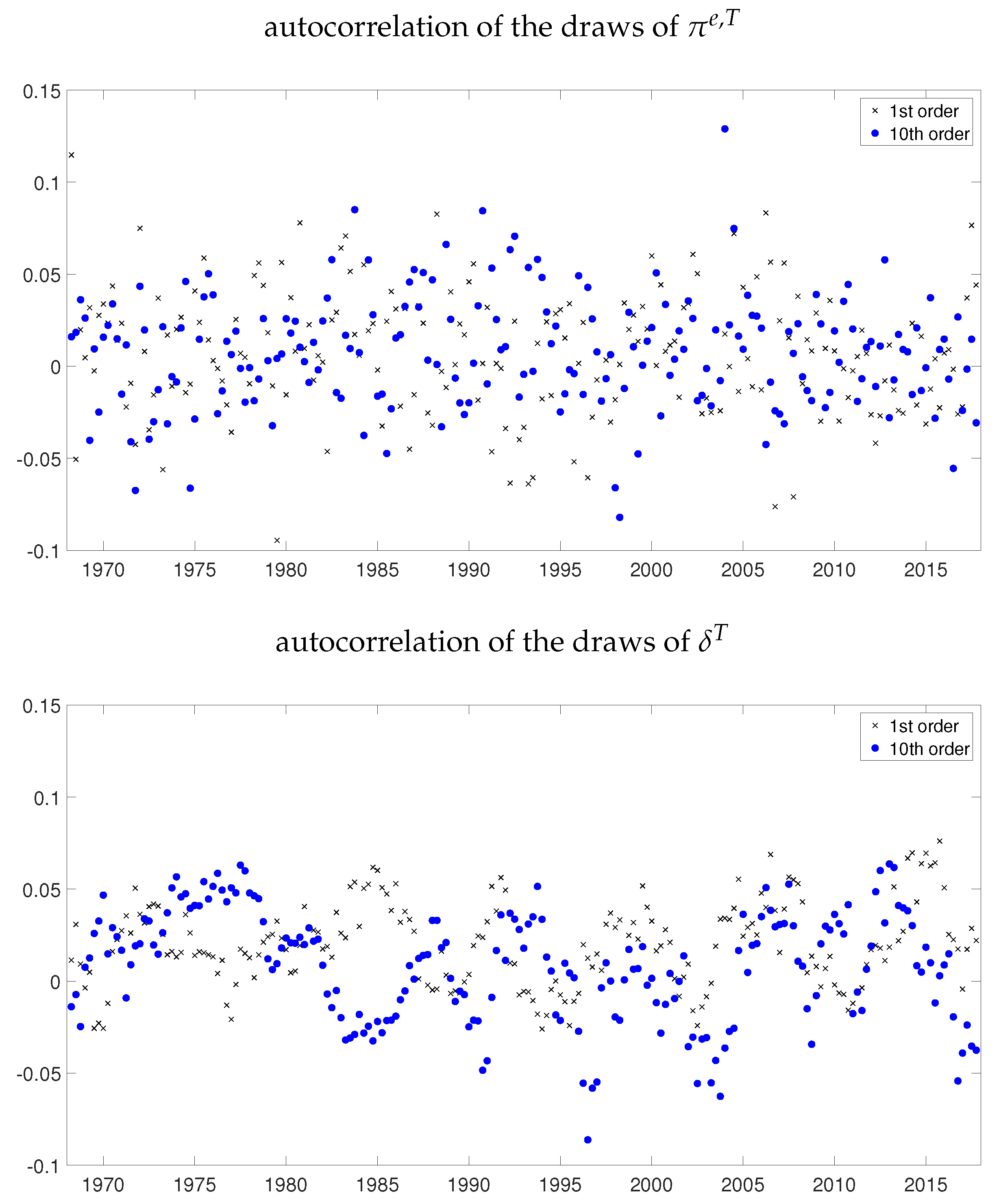
In order to further assess the convergence of the MCMC algorithm, I studied the autocorrelations of the draws. I first verified that the plots of the retained draws do not exhibit evident autocorrelation patterns. To substantiate the results of this graphical analysis, I then computed the autocorrelation functions of the draws. Below, I report the results for the 1st and 10th order autocorrelations; Table A1 refers to the parameters of the model and Figure A1 to each and in the histories and . All of these autocorrelations are very small, often smaller than 0.05 in absolute value, confirming that the convergence of the MCMC algorithm does not seem to be a reason for concern in this exercise.

Table A1.
Autocorrelations of the retained draws.
| 1st OrderAutocorrelation | 10th OrderAutocorrelation | |
|---|---|---|
| 0.0370 | 0.0409 | |
| 0.0719 | 0.0273 | |
| 0.0088 | −0.0003 | |
| 0.0283 | 0.0304 | |
| 0.0674 | 0.0034 | |
| 0.0754 | 0.0299 | |
| 0.0051 | 0.0524 |
Figure A1.
Autocorrelations of the retained draws.
References
- Baştürk, Nalan, Cem Çakmakli, S. Pinar Ceyhan, and Herman K. van Dijk. 2014. Posterior-Predictive Evidence On Us Inflation Using Extended New Keynesian Phillips Curve Models With Non-Filtered Data. Journal of Applied Econometrics 29: 1164–82. [Google Scholar] [CrossRef]
- Bernanke, Ben. 2010. The Economic Outlook and Monetary Policy. Speech delivered at the Federal Reserve Bank of Kansas City Economic Symposium, Jackson Hole, WY, USA, August 27. [Google Scholar]
- Binder, Carola Conces. 2015. Whose expectations augment the Phillips curve? Economics Letters 136: 35–8. [Google Scholar] [CrossRef]
- Blanchard, Olivier. 2016. The Phillips Curve: Back to the ’60s? American Economic Review 106: 31–4. [Google Scholar] [CrossRef]
- Blanchard, Olivier, Eugenio Cerutti, and Lawrence Summers. 2015. Inflation and Activity—Two Explorations and their Monetary Policy Implications. NBER Working Paper 21726, National Bureau of Economic Research, Cambridge, MA, USA. [Google Scholar]
- Carter, C. K., and R. Kohn. 1994. On Gibbs sampling for state space models. Biometrika 81: 541–53. [Google Scholar] [CrossRef]
- Chan, Joshua C. C., Todd E. Clark, and Gary Koop. 2015. A New Model of Inflation, Trend Inflation, and Long-Run Inflation Expectations. Working paper 15-20, Federal Reserve Bank of Cleveland, Cleveland, OH, USA. [Google Scholar]
- Cogley, Timothy, and Thomas J. Sargent. 2001. Evolving Post-World War II U.S. Inflation Dynamics. NBER Macroeconomics Annual 16: 331–73. [Google Scholar]
- Coibion, Olivier, and Yuriy Gorodnichenko. 2015. Is the Phillips Curve Alive and Well after All? Inflation Expectations and the Missing Disinflation. American Economic Journal: Macroeconomics 7: 197–232. [Google Scholar] [CrossRef]
- Coibion, Olivier, Yuriy Gorodnichenko, and Rupal Kamdar. 2017. The Formation of Expectations, Inflation and the Phillips Curve. NBER Working Papers 23304, National Bureau of Economic Research, Inc., Cambridge, MA, USA. [Google Scholar]
- Galì, Jordi. 2008. Monetary Policy, Inflation and the Business Cycle: An Introduction to the New Keynesian Framework. Princeton: Princeton University Press. [Google Scholar]
- Haubrich, Joseph G., George Pennacchi, and Peter H. Ritchken. 2008. Estimating Real and Nominal Term Structures Using Treasury Yields, Inflation, Inflation Forecasts, and Inflation Swap Rates. Working paper 08-10, Federal Reserve Bank of Cleveland, Cleveland, OH, USA. [Google Scholar]
- Kozicki, Sharon, and P. A. Tinsley. 2012. Effective Use of Survey Information in Estimating the Evolution of Expected Inflation. Journal of Money, Credit and Banking 44: 145–69. [Google Scholar] [CrossRef]
- Lopez-Perez, Víctor. 2017. Do professional forecasters behave as if they believed in the New Keynesian Phillips Curve for the euro area? Empirica 44: 147–74. [Google Scholar] [CrossRef]
- McCallum, Bennett T. 1976. Rational Expectations and the Estimation of Econometric Models: An Alternative Procedure. International Economic Review 17: 484–90. [Google Scholar] [CrossRef]
- Mertens, Elmar. 2016. Measuring the Level and Uncertainty of Trend Inflation. The Review of Economics and Statistics 98: 950–67. [Google Scholar] [CrossRef]
- Mertens, Elmar, and James M. Nason. 2017. Inflation and Professional Forecast Dynamics: An Evaluation of Stickiness, Persistence, and Volatility. CAMA Working Papers 2017-60, Centre for Applied Macroeconomic Analysis, Crawford School of Public Policy, The Australian National University, Canberra, Australia. [Google Scholar]
- Nason, James M., and Gregor W. Smith. 2013. Reverse Kalman Filtering U.S. Inflation with Sticky Professional Forecasts. Working Papers 13-34, Federal Reserve Bank of Philadelphia, Philadelphia, PA, USA. [Google Scholar]
- Nunes, Ricardo. 2010. Inflation Dynamics: The Role of Expectations. Journal of Money, Credit and Banking 42: 1161–72. [Google Scholar] [CrossRef]
- Primiceri, Giorgio E. 2005. Time Varying Structural Vector Autoregressions and Monetary Policy. The Review of Economic Studies 72: 821–52. [Google Scholar] [CrossRef]
- Primiceri, Giorgio E. 2006. Why Inflation Rose and Fell: Policy-Makers’ Beliefs and U. S. Postwar Stabilization Policy. The Quarterly Journal of Economics 121: 867–901. [Google Scholar] [CrossRef]
- Roberts, John. 1995. New Keynesian Economics and the Phillips Curve. Journal of Money, Credit and Banking 27: 975–84. [Google Scholar] [CrossRef]
- Staiger, Douglas, James H. Stock, and Mark W. Watson. 2001. Prices, Wages and the U.S. NAIRU in the 1990s. Working Paper 8320, National Bureau of Economic Research, Cambridge, MA, USA. [Google Scholar]
- Stock, James H., and Mark W. Watson. 2007. Why Has U.S. Inflation Become Harder to Forecast? Journal of Money, Credit and Banking 39: 3–33. [Google Scholar] [CrossRef]
- Stock, James H., and Mark W. Watson. 2016. Core Inflation and Trend Inflation. The Review of Economics and Statistics 98: 770–84. [Google Scholar] [CrossRef]
- Svensson, Lars E. O. 2015. The Possible Unemployment Cost of Average Inflation below a Credible Target. American Economic Journal: Macroeconomics 7: 258–96. [Google Scholar] [CrossRef]
| 1 | See Coibion and Gorodnichenko (2015) for a discussion of the interpretation of this variable in alternative structural models of the Phillips Curve. |
| 2 | The random walk process assumed in (3) is quite general, but other approaches to model long run inflation expectations within the context of the NKPC are also possible. For instance, see the framework used in Baştürk et al. (2014). |
| 3 | The natural rate of unemployment could also be estimated using a similar econometric model as the one employed for . However, treating both the natural rate and inflation expectations as unknown would have made the estimation of the full framework quite challenging. Given that the focus of this paper is on expectations, I decided to simply use the measure of the natural rate computed by the CBO and treat the variable as fully observable. |
| 4 | Monthly variables were transformed into quarterly by taking averages of the months in the quarter. The data for and were all downloaded from the FRED Federal Reserve Bank of St. Louis webpage. |
| 5 | Two additional exercises use the median forecast of price changes over the next 12 months for different demographic groups, and the median forecast of price changes over the next 5 to 10 years. As for the baseline series, these additional data were obtained from the University of Michigan Surveys of Consumers webpage and transformed into quarterly observations. |
| 6 | The methodology used to compute this series is described in Haubrich et al. (2008). |
| 7 | Equation (4) is not exactly the same as the one estimated by Coibion and Gorodnichenko (2015), because I do not include the indicator variable by itself as an additional variable. Thus, the model described by (4) is only able to capture a shift in the slope , but not in the intercept . This choice was forced by the fact that adding one more parameter considerably decreased the precision of all the estimated parameters of the NKPC. Thus, I decided to include the indicator variable only in the form of an interaction with which still allows the model to incorporate possible shifts in the slope of the NKPC, without increasing the dispersion of the estimates to a troublesome degree. |
| 8 | Notice that these are univariate Inverse Whisart distributions, which are equivalent to Inverse Gamma distributions. |
| 9 | I experimented with a range of different values for and for the mean in the prior for . I also tried to increase the dispersion of the Normal priors (8), (9), and (10), by multiplying the original variances by 4. Finally, I included factors and in (11) and (12) in addition to (13), and I experimented with different values for these factors. Neither the results nor the convergence of the algorithm were substantially affected by any of these changes. |
| 10 | The estimated value of is not statistically significant in Coibion and Gorodnichenko (2015) as well. |
| 11 | |
| 12 | For several of the inflation forecasts measures, the data are only available for some of these sub-periods. In each case, I only computed the statistics of interest if I had data for all the quarters in the sub-period. |
| 13 | |
| 14 | For more details, see Carter and Kohn (1994). |
Figure 1.
The estimated path of expectations. For each t, the figure reports the median of the retained posterior draws of (blue line), together with the 16th and 84th percentiles of the draws. The figure also reports the path of the inflation rate for comparison (dashed black line).
Figure 1.
The estimated path of expectations. For each t, the figure reports the median of the retained posterior draws of (blue line), together with the 16th and 84th percentiles of the draws. The figure also reports the path of the inflation rate for comparison (dashed black line).

Figure 2.
Expectations mistakes. For each t, the figure plots the difference between the actual inflation rate and the median of the draws of together with the 16th and 84th percentiles of this difference.
Figure 2.
Expectations mistakes. For each t, the figure plots the difference between the actual inflation rate and the median of the draws of together with the 16th and 84th percentiles of this difference.
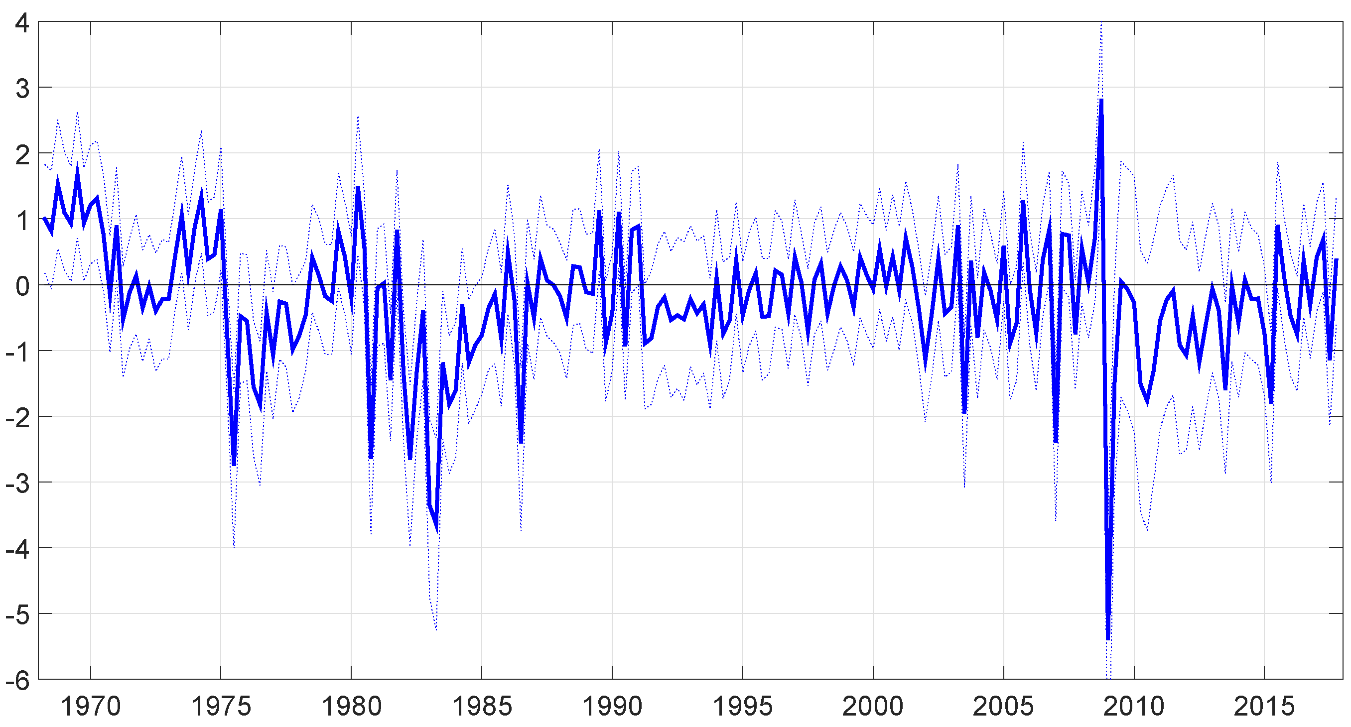
Figure 3.
The time-varying intercept. For each t, the figure reports the median of the retained draws of (red line), together with the 16th and 84th percentiles of the draws. The figure also reports the median of the retained posterior draws of (blue line).
Figure 3.
The time-varying intercept. For each t, the figure reports the median of the retained draws of (red line), together with the 16th and 84th percentiles of the draws. The figure also reports the median of the retained posterior draws of (blue line).

Figure 4.
The estimated and observable expectations, . For each t, the figure plots the median of the retained draws of (together with the 16th and 84th percentiles of the draws) and the measures of inflation forecasts described in the main text.
Figure 4.
The estimated and observable expectations, . For each t, the figure plots the median of the retained draws of (together with the 16th and 84th percentiles of the draws) and the measures of inflation forecasts described in the main text.
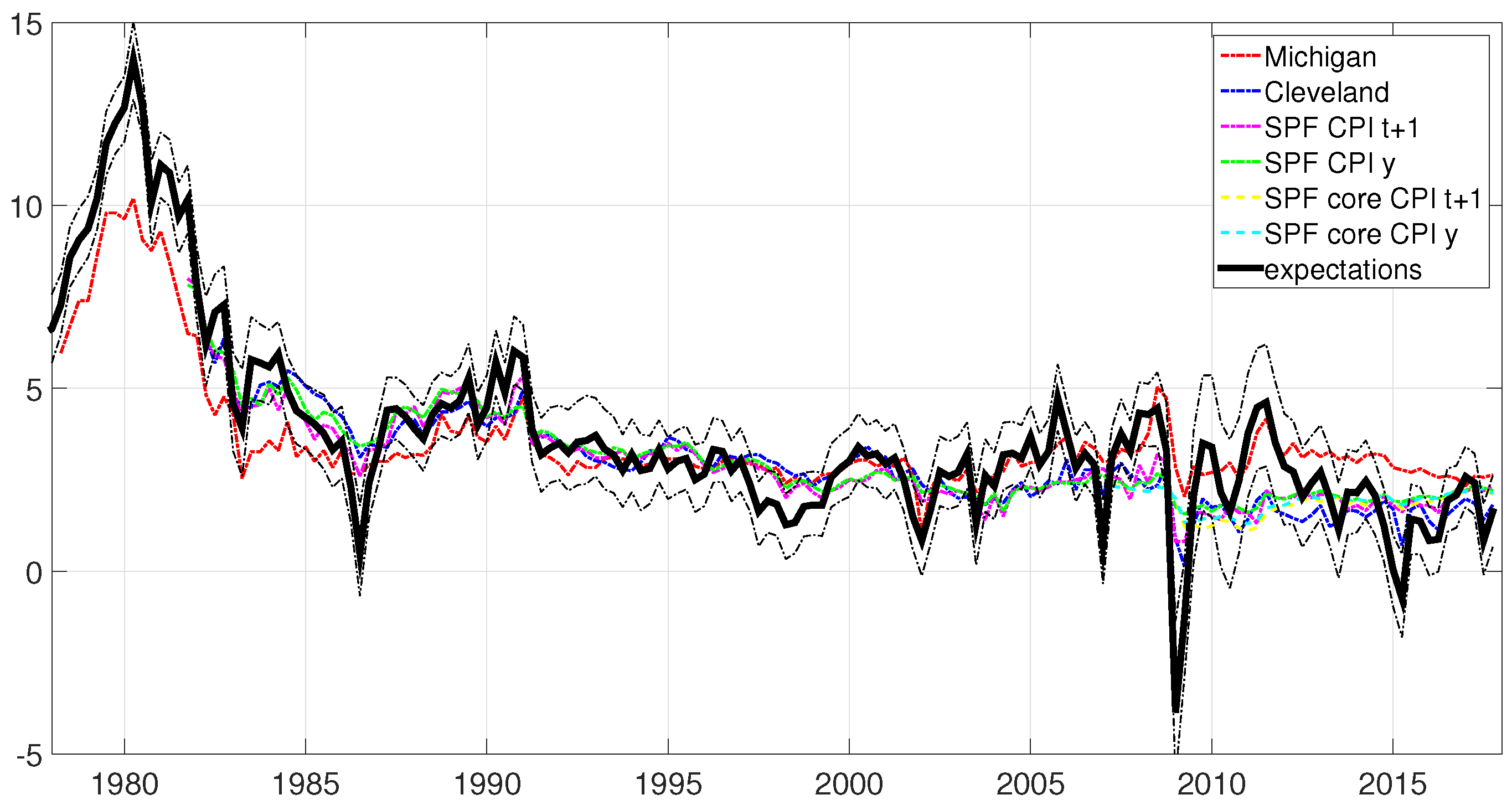
Figure 5.
The estimated and observable expectations, . For each t, the figure plots the median of the retained draws of (together with the 16th and 84th percentiles of the draws) and the measures of inflation forecasts described in the main text.
Figure 5.
The estimated and observable expectations, . For each t, the figure plots the median of the retained draws of (together with the 16th and 84th percentiles of the draws) and the measures of inflation forecasts described in the main text.
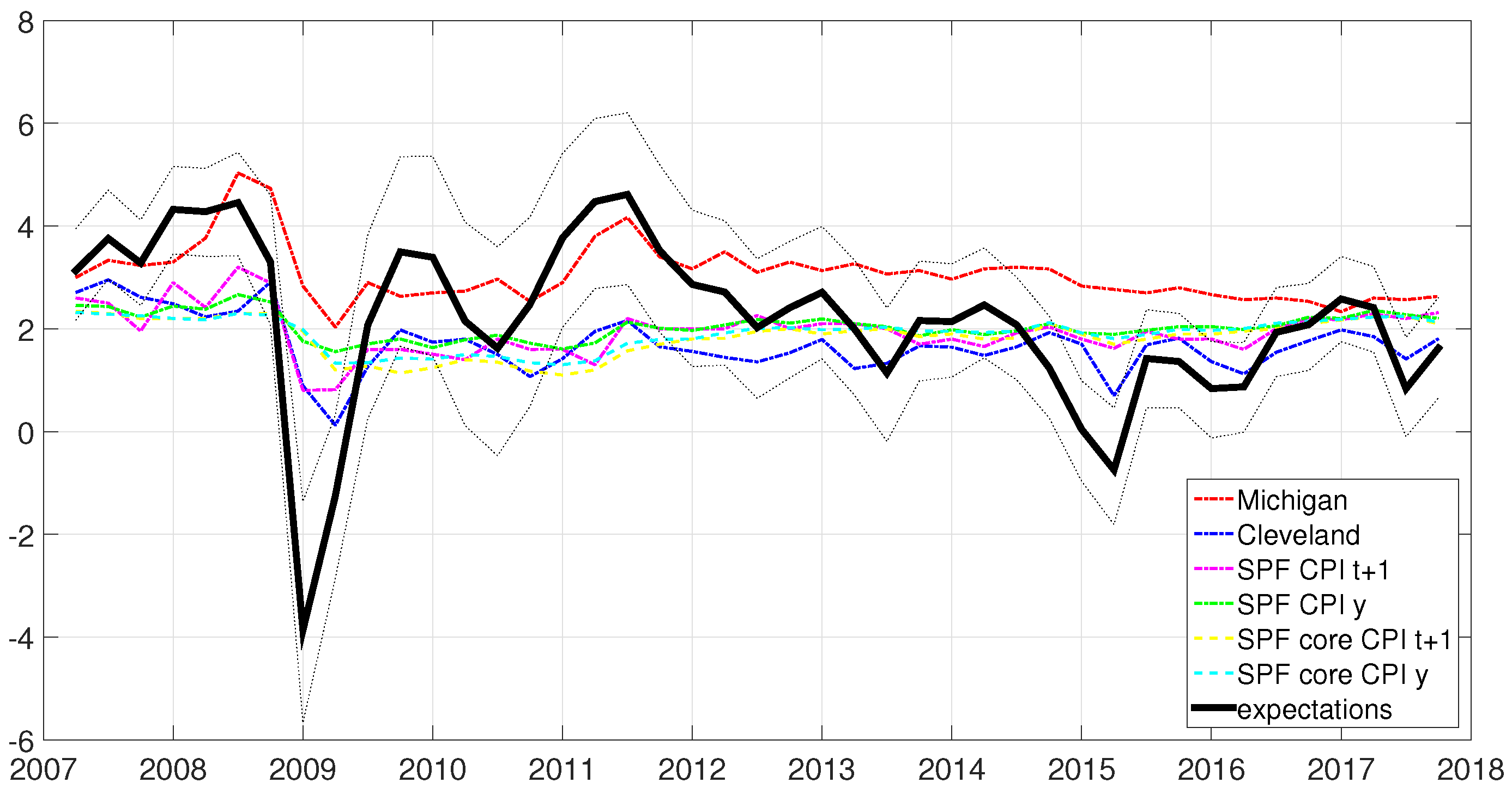
Table 1.
Estimated parameters of the model. The table reports the median, together with the 16th and 84th percentiles, of the 1000 retained posterior draws obtained from the MCMC estimation procedure.
Table 1.
Estimated parameters of the model. The table reports the median, together with the 16th and 84th percentiles, of the 1000 retained posterior draws obtained from the MCMC estimation procedure.
| 16th | Median | 84th | |
|---|---|---|---|
| −0.3075 | −0.0597 | 0.1461 | |
| −0.6963 | −0.4990 | −0.3246 | |
| −0.1570 | 0.2976 | 0.7105 | |
| 0.6881 | 0.7606 | 0.8508 | |
| 0.9464 | 1.2597 | 1.7059 | |
| 1.0767 | 1.9009 | 2.6421 | |
| 0.0113 | 0.0273 | 0.0554 |
Table 2.
Correlations between the estimated path of expectations and different measures of inflation forecasts, all available data. For each measure, the table reports the median, together with the 16th and 84th percentiles, of the 1000 correlations computed using the retained posterior draws of .
Table 2.
Correlations between the estimated path of expectations and different measures of inflation forecasts, all available data. For each measure, the table reports the median, together with the 16th and 84th percentiles, of the 1000 correlations computed using the retained posterior draws of .
| Correlations | Sample | 16th | Median | 84th |
|---|---|---|---|---|
| Michigan | 1978–2017 | 0.8414 | 0.8620 | 0.8830 |
| Cleveland | 1982–2017 | 0.5092 | 0.6459 | 0.7250 |
| SPF CPI (t) | 1981–2017 | 0.6967 | 0.7777 | 0.8185 |
| SPF CPI () | 1981–2017 | 0.5990 | 0.7065 | 0.7699 |
| SPF CPI (y) | 1981–2017 | 0.5564 | 0.6603 | 0.7359 |
| SPF core CPI (t) | 2007–2017 | −0.0625 | 0.1810 | 0.4196 |
| SPF core CPI () | 2007–2017 | −0.2842 | 0.0055 | 0.3203 |
| SPF core CPI (y) | 2007–2017 | −0.2712 | 0.0221 | 0.3395 |
Table 3.
Correlations between the estimated path of expectations and different measures of inflation forecasts; the sample is split in . For each measure, the table reports the median, together with the 16th and 84th percentiles, of the 1000 correlations computed using the retained posterior draws of .
| Correlations | Sample | 16th | Median | 84th | Sample | 16th | Median | 84th |
|---|---|---|---|---|---|---|---|---|
| Michigan | 1978–2006 | 0.8983 | 0.9128 | 0.9265 | 2007–2017 | 0.3823 | 0.4650 | 0.5370 |
| Cleveland | 1982–2006 | 0.5690 | 0.6415 | 0.7071 | 2007–2017 | 0.4175 | 0.6085 | 0.7325 |
| SPF CPI (t) | 1981–2006 | 0.7206 | 0.7630 | 0.7940 | 2007–2017 | 0.5877 | 0.7251 | 0.8095 |
| SPF CPI () | 1981–2006 | 0.6933 | 0.7442 | 0.7916 | 2007–2017 | 0.2634 | 0.4956 | 0.6755 |
| SPF CPI (y) | 1981–2006 | 0.6574 | 0.7145 | 0.7763 | 2007–2017 | 0.0586 | 0.3286 | 0.5771 |
| SPF core CPI (t) | - | - | - | - | 2007–2017 | −0.0625 | 0.1810 | 0.4196 |
| SPF core CPI () | - | - | - | - | 2007–2017 | −0.2842 | 0.0055 | 0.3203 |
| SPF core CPI (y) | - | - | - | - | 2007–2017 | −0.2712 | 0.0221 | 0.3395 |
Table 4.
Average, variance, and first order autocorrelation of the estimated path of expectations and different measures of inflation forecasts, all available data. For the estimated expectations, these statistics were computed using the median value of the 1000 retained posterior draws of .
Table 4.
Average, variance, and first order autocorrelation of the estimated path of expectations and different measures of inflation forecasts, all available data. For the estimated expectations, these statistics were computed using the median value of the 1000 retained posterior draws of .
| Average | Variance | Autocorrelation | |
|---|---|---|---|
| Sample period 1978–2017 | |||
| Estimated | 3.7903 | 7.4360 | 0.9188 |
| Michigan | 3.6138 | 2.8630 | 0.9554 |
| Sample period 1982–2017 | |||
| Estimated | 3.0425 | 2.3068 | 0.7468 |
| Cleveland | 2.9029 | 1.4444 | 0.9385 |
| Sample period 1981–2017 | |||
| Estimated | 3.1243 | 2.7763 | 0.7733 |
| SPF CPI (t) | 2.8799 | 2.6685 | 0.6252 |
| SPF CPI () | 2.9583 | 1.5487 | 0.9393 |
| SPF CPI (y) | 3.0597 | 1.5025 | 0.9788 |
| Sample period 2007–2017 | |||
| Estimated | 2.1912 | 2.6422 | 0.5640 |
| SPF core CPI (t) | 1.8103 | 0.1723 | 0.6025 |
| SPF core CPI () | 1.8383 | 0.1327 | 0.8820 |
| SPF core CPI (y) | 1.9094 | 0.0946 | 0.8898 |
Table 5.
Average expected inflation—the table reports the same information shown in Table 4, left column, but for different sub-periods.
Table 5.
Average expected inflation—the table reports the same information shown in Table 4, left column, but for different sub-periods.
| Average | 1978–1984 | 1985–2006 | 2007–2017 |
|---|---|---|---|
| Estimated | 8.3280 | 3.1279 | 2.1912 |
| Michigan | 6.2940 | 3.0295 | 3.0643 |
| Cleveland | - | 3.1651 | 1.7018 |
| SPF CPI (t) | - | 3.0346 | 1.8138 |
| SPF CPI () | - | 3.0678 | 1.9542 |
| SPF CPI (y) | - | 3.1531 | 2.0488 |
| SPF core CPI (t) | - | - | 1.8103 |
| SPF core CPI () | - | - | 1.8383 |
| SPF core CPI (y) | - | - | 1.9094 |
Table 6.
Variance of expected inflation rate—the table reports the same information shown in Table 4, middle column, but for different sub-periods.
Table 6.
Variance of expected inflation rate—the table reports the same information shown in Table 4, middle column, but for different sub-periods.
| Variance | 1978–1984 | 1985–2006 | 2007–2017 |
|---|---|---|---|
| Estimated | 8.8005 | 1.1633 | 2.6422 |
| Michigan | 6.3941 | 0.2493 | 0.3301 |
| Cleveland | - | 0.5958 | 0.3048 |
| SPF CPI (t) | - | 1.2955 | 2.0618 |
| SPF CPI () | - | 0.7813 | 0.2251 |
| SPF CPI (y) | - | 0.7306 | 0.0670 |
| SPF core CPI (t) | - | - | 0.1723 |
| SPF core CPI () | - | - | 0.1327 |
| SPF core CPI (y) | - | - | 0.0946 |
Table 7.
First order autocorrelation of the expected inflation series—the table reports the same information shown in Table 4, right column, but for different sub-periods.
Table 7.
First order autocorrelation of the expected inflation series—the table reports the same information shown in Table 4, right column, but for different sub-periods.
| Autocorrelation | 1978–1984 | 1985–2006 | 2007–2017 |
|---|---|---|---|
| Estimated | 0.9136 | 0.7582 | 0.5640 |
| Michigan | 0.9495 | 0.7061 | 0.6431 |
| Cleveland | - | 0.9179 | 0.5220 |
| SPF CPI (t) | - | 0.5604 | 0.3198 |
| SPF CPI () | - | 0.9129 | 0.5019 |
| SPF CPI (y) | - | 0.9677 | 0.7446 |
| SPF core CPI (t) | - | - | 0.6025 |
| SPF core CPI () | - | - | 0.8820 |
| SPF core CPI (y) | - | - | 0.8898 |
Table 8.
The table reports the correlations with the estimated expectations, the variances, and the autocorrelations, of two observable measures of expectations: “Michigan” and “Michigan 5 years”. “Michigan” refers to the measure used in the baseline analysis, i.e. the Michigan Survey “median forecast of price changes over the next 12 months”. “Michigan 5 years” is the Michigan Survey “median forecast of price changes over the next 5 to 10 years”. The results are presented for all the available data (1990–2017), and for two different sub-periods (1990–2006 and 2007–2017).
| 1990–2006 | 2007–2017 | 1990–2017 | |
|---|---|---|---|
| Correlation with | |||
| Michigan | 0.5851 | 0.4650 | 0.4722 |
| [16th, 84th] | [0.4931, 0.6574] | [0.3823, 0.5370] | [0.3904, 0.5253] |
| Michigan 5 years | 0.4695 | 0.3608 | 0.4091 |
| [16th, 84th] | [0.3489, 0.5816] | [0.2374, 0.4499] | [0.3422, 0.4800] |
| Variance | |||
| Estimated | 0.9228 | 2.6422 | 1.6963 |
| Michigan | 0.2204 | 0.3301 | 0.2648 |
| Michigan 5 years | 0.2294 | 0.0322 | 0.1842 |
| Autocorrelation | |||
| Estimated | 0.7279 | 0.5640 | 0.6347 |
| Michigan | 0.6597 | 0.6431 | 0.6579 |
| Michigan 5 years | 0.9672 | 0.7844 | 0.9602 |
Table 9.
The table reports the correlations between the estimated expectations and the Michigan Survey “median forecast of price changes over the next 12 months” for different demographic groups. For each group, the table reports the median, together with the 16th and 84th percentiles, of the 1000 correlations computed using the retained posterior draws of . The results are computed using all the available data for each group.
| Correlations | 16th | Median | 84th |
|---|---|---|---|
| 0.8414 | 0.8620 | 0.8830 | |
| Age groups (sample 1978–2017) | |||
| 18–34 | 0.8442 | 0.8658 | 0.8906 |
| 35–54 | 0.8528 | 0.8731 | 0.8938 |
| 55+ | 0.7654 | 0.7932 | 0.8152 |
| Regions (sample 1978–2017) | |||
| West | 0.8382 | 0.8593 | 0.8831 |
| North Central | 0.8263 | 0.8482 | 0.8685 |
| Northeast | 0.8522 | 0.8727 | 0.8912 |
| South | 0.8282 | 0.8499 | 0.8713 |
| Gender (sample 1978–2017) | |||
| Male | 0.8493 | 0.8693 | 0.8883 |
| Female | 0.8290 | 0.8514 | 0.8732 |
| Income group (sample 1979–2017) | |||
| Bottom 33% | 0.7315 | 0.7617 | 0.7853 |
| Middle 33% | 0.7913 | 0.8160 | 0.8401 |
| Top 33% | 0.8189 | 0.8452 | 0.8675 |
| Education level (sample 1978–2017) | |||
| High School or less | 0.7908 | 0.8175 | 0.8383 |
| Some college | 0.8186 | 0.8410 | 0.8614 |
| College degree | 0.8576 | 0.8790 | 0.9014 |
© 2018 by the author. Licensee MDPI, Basel, Switzerland. This article is an open access article distributed under the terms and conditions of the Creative Commons Attribution (CC BY) license (http://creativecommons.org/licenses/by/4.0/).
Share and Cite
MDPI and ACS Style
Rondina, F. Estimating Unobservable Inflation Expectations in the New Keynesian Phillips Curve. Econometrics 2018, 6, 6. https://doi.org/10.3390/econometrics6010006
AMA Style
Rondina F. Estimating Unobservable Inflation Expectations in the New Keynesian Phillips Curve. Econometrics. 2018; 6(1):6. https://doi.org/10.3390/econometrics6010006
Chicago/Turabian StyleRondina, Francesca. 2018. "Estimating Unobservable Inflation Expectations in the New Keynesian Phillips Curve" Econometrics 6, no. 1: 6. https://doi.org/10.3390/econometrics6010006
Note that from the first issue of 2016, this journal uses article numbers instead of page numbers. See further details here.