A Multivariate Kernel Approach to Forecasting the Variance Covariance of Stock Market Returns


1
Economics, School of Social Sciences, University of Manchester, Oxford Road, Manchester M13 9PL, UK
2
School of Economics and Finance, Queensland University of Technology, Brisbane City, QLD 4000, Australia
3
The Business School, University of Huddersfield, Huddersfield HD1 3DH, UK
*
Author to whom correspondence should be addressed.
Econometrics 2018, 6(1), 7; https://doi.org/10.3390/econometrics6010007
Submission received: 29 September 2017
/
Revised: 30 January 2018
/
Accepted: 13 February 2018
/
Published: 17 February 2018
(This article belongs to the Special Issue Volatility Modeling)
Abstract
:This paper introduces a multivariate kernel based forecasting tool for the prediction of variance-covariance matrices of stock returns. The method introduced allows for the incorporation of macroeconomic variables into the forecasting process of the matrix without resorting to a decomposition of the matrix. The model makes use of similarity forecasting techniques and it is demonstrated that several popular techniques can be thought as a subset of this approach. A forecasting experiment demonstrates the potential for the technique to improve the statistical accuracy of forecasts of variance-covariance matrices.
JEL Classification:
C53; C581. Introduction
Forecasting variance-covariance matrices (VCMs) is an important issue in finance, having applications in portfolio selection and risk management as well as being directly used in the pricing of several financial assets. In recent years an increasing body of literature has developed multivariate models to forecast this matrix, these include the DCC of Engle and Sheppard (2001), the VARFIMA model of Chiriac and Voev (2011) and Riskmetrics of J.P. Morgan (1996). All of these models can be used to forecast the VCM of a portfolio and do so only using returns data from the assets under consideration.
Previous studies, focusing on modelling the volatility of single assets, have identified economic predictor variables that may be related to the variance of returns and attempted to utilise such variables in forecasting. For example Aït-Sahalia and Brandt (2001) investigate which of a range of factors influence stock volatility such as dividend yields and default spreads. However, advances in terms of multivariate volatility models are complicated by the requirement that forecasts of VCMs must be positive semi-definite (psd) and symmetric, restrictions which make the incorporation of predictor variables difficult. As the dimension of the problem increases two issues arise. First, without complex restrictions this will result in a proliferation of parameters, making identification and estimation difficult. Second, the implicit assumption of model stability becomes less defendable as the model dimension grows.
In this paper a semi-parametric kernel based forecasting method is proposed where forecasts are based on a weighted average of past observations of VCMs. This approach builds on the work by Clements et al. (2011), who show that in a univariate setting, employing kernels to determine weighting structures dependent on the similarity of volatility observations through time can improve forecast accuracy when compared to more established methods. As this essentially generates VCM forecasts as weighted averages of past VCMs it guarantees symmetry and positive-semi-definiteness by construction and hence avoid the issues discussed earlier.
The proposed method is similar in spirit to Riskmetrics forecasts and the Heterogeneous Autoregressive (HAR) model of Corsi (2009)1. However the proposed approach does not make the potentially restrictive assumption that more recent observations attract a larger weight, with the weights being a decreasing function of the time difference between when the forecast is formed and the time at which a VCM was observed2. Additionally, the impact of predictor variables are easily included within the kernel weighting function while avoiding the problems discussed above that are commonly encountered with multivariate models. The methodology proposed here is merely a forecasting tool. It is not meant to represent an underlying data generating process. It is therefore understood that, as a representation of the unknown data generating process it is surely misspecified. Its value lies in (potentially) improved forecast quality.
An empirical analysis is undertaken to examine the efficacy of the proposed forecasting framework. Given the nature of the approach, and the potentially wide range of exogenous variables, it is not straightforward to design a representative simulation experiment. As a result, a thorough and careful forecasting exercise is undertaken, focusing on forecasting the variance-covariance matrix of the returns on 20 large U.S. stocks. A range of predictor variables including matrix similarity measures, interest rate information, commodity returns, and a range of macroeconomic data and option implied volatility are used.
This empirical analysis is designed to address a number of issues. Does the proposed forecasting approach compare favourably to more established forecasting techniques for relatively high dimensional VCMs? Do the predictor variables help improve the accuracy of VCM forecasts? And finally, do the use of matrix comparison measures lead to improved forecasting performance? Overall, the results of the forecasting experiment are promising in that they establish that the proposed non-parametric approach produces forecasts of the VCM that are statistically superior to those from a range of competing models. The results also demonstrate that the variables which measure the similarity of VCM realisations can significantly improve on forecasts based only on kernels that are a function of time. However, there is little evidence to show that using any of the other variables adds significantly to forecast performance.
The paper proceeds as follows. Section 2 introduces important terminology and notation and offers an overview of the current forecasting approaches including the role played by exogenous predictor variables. Section 3 shows how a number of common forecasting methods can be expressed as a kernel based approach. Section 4 outlines the methodology underlying the proposed forecasting approach. Section 5 describes the data used in the empirical analysis. Section 6 outlines the structure of the empirical analysis including the forecasting exercise and the competing models. Section 7 and Section 8 report the results of the empirical analysis focusing on the behaviour of the kernel weighting functions and forecast performance respectively. Section 9 provides concluding comments.
2. Background
This section will discuss the framework on which this paper builds. Important notation and terminology will be presented followed by an outline of the existing approaches to forecasting the VCM.
2.1. Notation and Terminology
The approach presented here is used to forecast the volatility of stock returns at a daily frequency for an n stock portfolio. For a given trading day, the vector of returns is denoted by where is the return on stock i on day and it is assumed that given all information available at time , . The object of interest is the positive-definite variance-covariance matrix of returns, which is assumed to be time-varying, predictable, and although unobserved, consistently estimated by a realized variance-covariance matrix . In this paper represents the true but unobservable VCM, denotes an observed realized measure of the VCM, calculated from intraday data, and is used to denote a forecast of the matrix.
A realized estimate of is made possible by the availability of intra-day returns data but estimation is complicated by the presence of micro-structure noise, non-synchronous trading and the need for to be positive semi-definite (psd). Here the multivariate realised kernel estimator of Barndorff-Nielsen et al. (2011) is employed which takes into account microstructure noise, non-synchronous trading at the same time guaranteeing a psd estimate. The estimation of under the approach is supported by a literature of its own right and will not be discussed further here3.
2.2. Approaches to Modelling the VCM
The multivariate volatility modelling literature continues to be an active field of research. There is a well established literature on multivariate GARCH-type models, see Silvennoinen and Teräsvirta (2009) for a comprehensive review. Given the focus here is on forecasts using , GARCH models will be not be discussed further. Models for the realized variance-covariance matrix (rVCM) share a common starting point in that they treat the unique elements of as observed, rather than having to infer them from n observed returns, which is the approach of GARCH models. A simple approach to forecasting would be to apply standard multivariate time-series models (e.g., a Vector Autoregressive Model, VAR) to the observed unique elements of the rVCM. However, this approach will potentially deliver forecasts that are not psd. A number of approaches exist to deal with this issue, including the method proposed here.
A useful approach for guaranteeing psd forecasts is to deal with a decomposition of the rVCM. Standard multivariate time-series models can be applied to the elements of the decomposition and subsequently reverse the decomposition to obtain forecasts for the rVCM, guaranteeing the resulting rVCM forecast is psd. Two different decompositions have been proposed in this context. Chiriac and Voev (2011) use a Cholesky decomposition to obtain a set of variables they were then free to model with a standard VARFIMA approach before reversing the decomposition. Bauer and Vorkink (2011) model latent factors of the matrix logarithm of the rVCM, a process which once again can be reversed to guarantee a psd forecast. The factors are driven by past volatility along with exogenous predictor variables. While these are interesting approaches and avoid concerns regarding positive-semi definiteness of the forecasts, the role of predictor variables are difficult to interpret in such a framework as the decomposed elements of the matrices are not easily related to the elements of the original VCM.
Golosnoy et al. (2012) find an alternative way to meet the restriction that the resulting variance-covariance matrix needs to be positive-semi definite by allowing the covariance matrix to follow a conditional central Wishart distribution. The scale matrix in the context of the central Wishart distribution is modelled as a linear function of past realizations and forecasts of the rVCM matrices and positive definiteness is guaranteed with trivial restrictions on the initial matrices used in the model4.
The simplest way to obtain psd forecasts of the rVCM is to produce forecasts by merely averaging past observations of the rVCM, which by construction, are psd themselves. The Riskmetrics approach to forecasting the variance-covariance matrix is based on this principle with an exponentially weighted moving average (EWMA) applied to the history of . Fleming et al. (2003) use a similar weighting scheme applied directly to in order to demonstrate the economic benefit of forecasting using RVCMs as opposed to daily returns. The use of the EWMA scheme imposes decaying weights. A recent approach gaining popularity is the Heterogeneous Autoregressive (HAR) model of Corsi (2009) which can be applied to forecasting the rVCM. Similar to the Riskmetrics approach, the weights in a HAR model decline with time but as a step function rather than smoothly. As shown by Chiriac and Voev (2011) and Bauer and Vorkink (2011), HAR models can be applied to the transformed elements (Cholesky or Matrix Logarithm transformation) of the rVCM. This is appealing as it facilitates the straightforward estimation of rather complex dynamics of these elements which in turn can be used to produce psd forecasts (see details in Section 6.2).
The approach proposed here generates forecasts that are weighted averages of previously observed rVCMs. However the weight applied to past observations of the rVCM is not solely determined by the lags at which it is observed. This approach builds upon Clements et al. (2011) who developed a univariate volatility forecasting scheme, where forecasts are a weighted average of historical values of realized volatility and the weights are related to the similarity between historical volatility and volatility at the time at which the forecast is formed. Clements et al. (2011) show that at a 1 day forecast horizon such an approach performs well against competing volatility forecasting techniques.
This principle is extended to the multivariate setting in this paper with a kernel based approach proposed for forecasting the VCM and is an application of the general technique of empirical similarity, as described more generally in Gilboa et al. (2006). The kernel density acts as a similarity function and the forecasts of the rVCM are similarity weighted averages. This technique allows for the weights to be determined by a vector of variables rather than only one variable (e.g., time difference as in the Riskmetrics or HAR models). It is notable that the only previous explicit use of similarity forecasting in volatility forecasting is in Golosnoy et al. (2014) who used the general approach to combine univariate forecasts of stock return volatility using similarity based weights which compare the forecast period to previous periods, in this case similarity is computed based on the closeness of forecasts of models of the value of volatility at the current forecast point. It is shown that the proposed method encompasses Riskmetrics as a special case5.
2.3. The Role of Predictor Variables
The basic idea of using variables that describe macroeconomic or market conditions in making forecasts is to give larger weights to past rVCMs from periods which have conditions that are similar to those prevalent at the time of forming the forecast. A wide range of such variables have been considered in the context of mainly univariate models for volatility. Building on earlier work, Aït-Sahalia and Brandt (2001) consider dividend yield, default spreads and term spreads. Campbell (1987), Fama and French (1989) and Harvey (1991) investigate the relationship between term spreads and volatility while Fama and French (1989), Whitelaw (1994) and Schwert (1989) consider a volatility-default spread relationship. In addition Harvey (1989) considers the impact of default spreads on covariances. Hence there is an established literature relating these variables to the behaviour of elements of a VCM.
Empirical evidence in Schwert (1989), Hamilton and Lin (1996), and Campbell et al. (2001) suggests that during market downturns/recessions stock return volatility can be expected to increase. Therefore, the algorithm of Pagan and Sossounov (2003) is used to identify periods in bullish/bearish periods in the stock market, as VCMs in such periods may have common characteristics. Commodity prices, such as gold (Sjaastad and Scacciavillani 1996) and oil (Sadorsky 1999; Hamilton 1996) prices, have also been linked to stock market volatility and are therefore considered here as potential variables to contribute to the kernel weighting functions.
The final variable that falls into this category is implied volatility, namely the VIX index of the Chicago Board of Exchange. This is often interpreted as a market’s view on future stock market volatility. This measure has been used in the context of univariate volatility forecasting (Poon and Granger 2003; Blair et al. 2001) and is here considered as another variable in the multivariate kernel weighting scheme.
Another important class of variables considered for the kernel weighting algorithm are scalar transformations of matrices as they can be used to establish the closeness or similarity of matrices. The idea is to give higher weight to past observations from periods when the rVCM was similar to the current rVCM (regardless of how distant in time that observation is). To the best of our knowledge such variables have not previously been used in the context of VCM forecasting. There is, however, a literature that discusses matrix distance measures. Moskowitz (2003) proposes three statistics to evaluate the closeness of rVCMs. The first metric compares the matrix eigenvalues, the second looks at the relative differences between the individual matrix elements and the third considers how many of the correlations have the same sign in the matrices. These three metrics will be utilised to determine the level of similarity between two rVCMs. Other functions used to compare matrices, often called loss functions, have been discussed in the forecast evaluation literature (for example in Laurent et al. 2013). One such loss function is the Stein distance, also known as the MVQLIKE function6. This loss function is shown to perform well in discriminating between VCM forecasts in Becker et al. (2014) and Laurent et al. (2012) and represents another useful tool for comparing VCMs.
3. Riskmetrics and HAR Models Interpreted as Kernel (Similarity) Based Forecasts
Commonly used forecasting approaches can be interpreted as a kernel or a similarity based approach. It is therefore related to the more general methodology introduced in Section 5 in which a multivariate kernel is introduced which potentially utilises several exogenous variables. In this section a result by Gijbels et al. (1999) is restated that establishes that a Riskmetrics type, exponential smoothing forecast can be represented as a univariate kernel forecast in which weights vary with time.
In a multivariate setting, the standard Riskmetrics forecast, at time T is given by
when observations are equally spaced in time and is a smoothing parameter, commonly set at a value recommended in J.P. Morgan (1996). From recursive substitution and with , the forecast of the VCM can be expressed as
The sum of the weights is equal and as noted in Gijbels et al. (1999) which approaches 1 as T approaches infinity. However in order to normalise the sum of the weights to be exactly 1, the Riskmetrics model can be restated as
which can reformulated with kernel weights7, defining and , allowing (3) to be restated as
This replicates the conclusion of Gijbels et al. (1999) that Riskmetrics is a zero degree local polynomial kernel estimate with bandwidth h. From a practical point of view the Riskmetrics kernel determines weights, , are based on how close observations of are to time T, the period at which a forecast is being made. The largest weight is attached to the observation at time T with the weights exponentially decaying.
In the univariate volatility context, the HAR model is based on a step kernel, rather than the smoothly decaying kernel built under the Riskmetrics approach. In the context of multivariate forecasting the application of either Riskmetrics or HAR is hampered by the fact that the estimation of kernel bandwidths is not straightforward. This is the reason why Riskmetrics approaches tend to be applied with fixed, pre-determined bandwidths. However, it is argued here that a bandwidth can be estimated with a cross-validation approach. It is useful to demonstrate that the Riskmetrics model can be represented as a kernel based model as this highlights that the basic methodology proposed here encompasses existing popular methods, while at the same time including measures of closeness of dimensions other than time. While this may be the case, empirical results show that time based weighting remains important.
4. Methodology
This section presents the method by which the kernel weighting scheme and subsequent forecasts of the VCM are obtained. The inputs are a set of p variables, which may contain information relevant to forecasting the VCM and a time series of rVCMs. Calculation of the rVCM, , is a non-trivial issue. Here it is computed using two standard methods from the realized (co)variance literature and it is assumed that is psd. The method used to calculate the matrices used in the rest of this paper is now described.
4.1. Calculation of Realised Variance Covariance Matrices
The estimate is treated as an observed estimate of the integrated covariance (e.g., Christensen et al. 2010; Barndorff-Nielsen et al. 2011). The methods to achieve this are now summarised. For any given trading day, the vector of returns is denoted by where is the return on stock i on day t. Also for day t there are M vectors of synchronised intra-day returns for 8.
The calculation of is accomplished along the lines proposed by Barndorff-Nielsen et al. (2011), producing a multivariate realised kernel (MVRK) estimate9.
Both the kernel function and the bandwidth, H, are chosen in the manner recommended in Barndorff-Nielsen et al. (2011). The kernel is the Parzen kernel and the bandwidth is estimated from the data. Importantly, this estimate will produce a positive semi-definite matrix that allows for non-synchronous trading and the existence of some microstructure noise10.
4.2. Kernel Approach to Forecasting
Assume that at time T a forecast of the d step ahead VCM from to , denoted by is required11. The forecasts is obtained by taking a weighted average of past rVCMs,
As this is a weighted combination of symmetric, psd matrices, also inherits these properties and so is a valid covariance matrix without resorting parameter restrictions or transformations. As discussed in Section 3 the Riskmetrics and HAR forecasting models can be seen as special cases of this approach.
The focus of much of the remainder of this section is a description of how the optimal weights in (5), are found. In order to ensure that the weights sum to one the following normalisation is imposed,
which allows Equation (5) to be interpreted as a weighted average, ensuring an appropriate scaling for .
The central idea is to determine which of the past time periods experienced conditions most similar to those at the time of forming the forecast, T, a logic based on the similarity forecasting approach framework of Gilboa et al. (2011). More weight is placed on the VCMs that occurred over the d periods following the dates that were most similar to time T, the forecast point. The similarity of historical periods to time T is determined using p variables and employs a multivariate kernel to calculate the raw weight applicable to day t, hence
where is the element from the row and column of the dimensional data matrix which collects all T observations for the p potential weighting variables is the bandwidth for the variable.
For continuous variables is the standard normal density kernel12 (Silverman 1986; Bowman 1997) defined as
In the case of a discrete variable, such as a bull/bear market dummy used below, the discrete univariate kernel proposed by Aitchison and Aitken (1976) is used. The form of the kernel is
where is the number of possible values the discrete variable can take ( in the case of the bull/bear market variable). In the two state discrete case . If the value of the discrete variable has no impact on the forecast, while if we disregard data points which do not share the same discrete variable value as .
As discussed earlier, it is possible to think of several time based approaches to forecasting , thus a kernel based on Riskmetrics weighting is used here to explicitly account for time When time is included as one of the p variables the kernel with the form,
is employed, which has the same structure as the Riskmetrics approach in Equation (3). However, here a flexible bandwidth, , is allowed as opposed to a pre-specified value as in J.P. Morgan (1996). This time kernel will generally tend to produce weighting patterns for time which are similar to those produced by other exponential smoothing approaches. The largest weights will be placed on the most recent observations of the realized VCM and will generally fall away to zero quickly. This is important in the multivariate kernel as the multiplicative nature of Equation (7a) means that this property will be inherited by the weights used in the multivariate kernel. While the general approach presented through Equations (5), (6) and (7a) captures the Riskmetrics approach as a special case, it introduces a significant amount of additional flexibility, by allowing the weights to be determined from a set of p variables other than just time13.
4.3. Cross Validation Optimisation of Kernel Bandwidths
The choice of bandwidth is a non-trivial issue in non-parametric econometrics, however a common rule of thumb quoted for multivariate density estimation is
where is the standard deviation of the variable. Although this rule of thumb provides a simple method for choosing bandwidths, as noted in Wand and Jones (1995) these bandwidths may be sub-optimal.
Importantly, if one was to optimise (using cross-validation) the bandwidth parameters, the optimised bandwidths , will reflect the importance of the jth element in for determining the optimal weights . As noted in Li and Racine (2007, pp. 140–41), irrelevant (continuous) variables are associated with . For binary variables (and kernel as in Equation (7c)) and a time variable (and a kernel as in Equation (7d)) the bandwidths and respectively represent irrelevant variables.
Cross-validation is a bandwidth optimisation strategy introduced by Rudemo (1982) and Bowman (1984). It selects bandwidths to minimise the mean integrated squared error (MISE) of density estimates and is generally recommended as the method of choice in the context of non-parametric density and regression analysis (see Wand and Jones 1995; Li and Racine 2007). As forecast performance rather than density estimation is of interest here, the bandwidths are obtained by minimising the MVQLIKE of the forecasts. Alternative loss functions, such as MSE are available, however they are not considered as most are not robust to estimation error in the volatility estimates, see Patton and Sheppard (2009). This choice is discussed further in Section 8.1.
4.3.1. Cross-Validation Criterion and Setup
MVQLIKE is a robust loss function for the comparison of matrices14, where is the dimensional 1 period ahead forecast of the VCM at time t and is the realized VCM at time t15. The notation makes it explicit that the forecasts are a function of the bandwidth vector h. The loss function is defined as
which is to be minimised during cross-validation.
There is data available up to and including time period T and the aim is to forecast the VCM for . The available data over time periods 1 to T can be used to identify the optimal bandwidths for use in forecasting. This is done by evaluating forecasts for periods to T. At any given bandwidth h the initial observations 16 are used to produce the first forecast . For any period , , the forecast is based on observations of variables in available at time .
A non-linear optimisation algorithm then determines the bandwidths that minimise the mean of MVQLIKE over these in-sample forecasts
4.3.2. Practical Implementation
The optimised bandwidths reflect how the p variables included in contribute to the determination of the weights in Equation (5). This aspect of the bandwidth parameter has also been pointed out by Gilboa et al. (2011) in the context of similarity forecasts. Li and Racine (2007) suggest that a cross-validation approach in the context of a multivariate kernel regression should, asymptotically, deliver bandwidth estimates that approach their irrelevant values discussed above (, and respectively for continuous, binary and time variables), meaning there should be no need to manually eliminate irrelevant variables.
To begin, when all variables were considered jointly, difficulties were encountered in the optimisation process and the non-linear bandwidth optimisation of (9) was unable to identify an optimum.
An alternative strategy is proposed in which first attempts to eliminate variables that contribute little to improving forecasts, before identifying optimal bandwidths only for the remaining subset of variables. This is achieved as follows. Each variable is used as the individually in to determine kernel weights.
The optimal bandwidth, , for each variable is found by minimising the criterion in (9). The optimal is then compared to a benchmark from taking simple moving averages of past VCMs to form a forecast. The rationale is that a relevant variable should deliver improvements compared to a naïve approach. Weighting variables that do not improve on the by at least 1% are then eliminated17.
In short the process of variable elimination and bandwidth optimisation can be summarised in the following three step procedure:
- For each of the p variables considered for inclusion in the multivariate kernel, apply cross validation to obtain the optimal bandwidth when only that variable is included in the kernel estimator. These are referred to as univariate optimised bandwidths .
- Compare the forecasting performance of the univariate optimised bandwidths from Step 1, , against from a simple moving average forecast model. Any of the p variables that fail to improve on the rolling average forecast performance by at least 1% are eliminated at this stage as it is considered to have little value for forecasting. We are left with variables used as weighting variables.
- Estimate the multivariate optimised bandwidths for the variables that are not eliminated in Step 2 by minimising the cross validation criterion in Equation (9). As opposed to Step 1 this optimisation is done simultaneously over all bandwidths.
5. Data
The stock return data and additional predictor variables used are now outlined. The predictor variables can be grouped into two classes, namely those which are based on observations of the variance-covariance matrix and those which represent exogenous macroeconomic variables. All models considered below also make use, either explicitly or implicitly, of a time variable which is defined as the number of trading days between two points in time.
5.1. Stock Data
The empirical analysis is based on a portfolio of 20 large stocks traded on the New York Stock Exchange (NYSE) from across a variety of industries. Intra-day price data is obtained from the NYSE Trade and Quote database via the Wharton Research Data Service for the period covering 02/01/1997-31/12/2012. This delivers 4,026 trading days with information. Appendix A lists the 20 stocks included in the analysis18.
This data is used to create realisations of the variance-covariance matrix, , as described in Section 4.119. These realisations of the VCM are then used in creating the variables which are based on comparisons of the elements of the matrix which are then included in the kernel model.
5.2. Weighting Variables
5.2.1. Matrix Comparison Variables
Moskowitz (2003) discusses a range of statistics that measure the difference between two covariance matrices. Three of these statistics are considered here as they provide a direct comparison of matrices. The first measure is the ratio of the eigenvalues of the variance covariance matrix at time t relative to those of the VCM at time T (EigValues):
Values closer to 1 indicate that a greater degree of similarity. The second statistic, adopted from Moskowitz (2003), evaluates the absolute element-wise differences between the matrices and . The sum of all absolute differences is standardised by the sum of all elements in (ElemDiff). The statistic is defined as
where is an vector of ones. For identical matrices this statistic will take a value of 0.
This makes use of the realized correlation matrices and 20. is an indicator taking the value of 1 when the statement inside the brackets is true and 0 otherwise and is the number of unique correlations in the correlation matrix. Equation (12) compares how similar and are in relation to the average realized correlation matrix . This measure compares correlations to their long run-average values. delivers a positive (negative) sign if the realized correlation (of the unique element) at time t is larger (smaller) than the relevant average correlation. The statistic considered here essentially calculates the proportion of the m unique elements in that have identical patterns of deviations from the long-run correlations as those in (SignDiff). If matrices are identical with respect to this measure this statistic will take a value of 1.
The weighting scheme also employs a comparison of matrices using the MVQLIKE loss function (Laurent et al. 2012) due to it being a robust multivariate loss function (as well as playing a key role in the cross validation procedure), defined as
such that matrices which are identical will deliver a statistic of value 0. These four statistics are used to measure the degree of similarity between the VCMs at time t and time T. The variable selection and bandwidth estimation strategy described previously will determine which of these variables are relevant for VCM forecasting.
5.2.2. Economic Variables
The variables introduced in this section form the set of predictor variables, chosen, based on findings in the existing volatility forecasting literature. The variable is the term spread, used in Aït-Sahalia and Brandt (2001) and defined as the difference between 1 and 10 year US government bond yields21. Aït-Sahalia and Brandt (2001) also investigated the relation between return volatility and default spread, given by the difference in yield between Moody’s Aaa and Baa rated corporate bonds at time t 22.
Both oil prices and gold prices have been shown to influence stock return volatility (Sjaastad and Scacciavillani 1996; Sadorsky 1999; Hamilton 1996), based on this we include daily price levels of both of these commodities in the set of kernel variables2324. While this means that the set of variables will include non-stationary variables, there is no reason why such variables can not be included in the kernel approach.
Schwert (1989), Hamilton and Lin (1996) and Campbell et al. (2001) demonstrate that volatility increases during economic downturns. This motivates the use of a dummy variable identifying bull and bear market periods as described in Pagan and Sossounov (2003)25. When constructing this variable26, only historical information is used in determining turning points between states of the market and hence this can be used for forecasting purposes. The variable is defined as having a value of one when the market is bullish and 0 otherwise and is the only variable which uses the discrete kernel described above.
As this model is focused on the volatility of a stock portfolio it may also be useful to include a market-wide measure of volatility in the list of potential variables. In order to do this the volatility index (VIX) level quoted by the Chicago Board Options Exchange is used as one of the variables across which time periods are compared27.
While no simulation study is undertaken, as a test of the efficacy of this approach, two irrelevant variables are included which should be excluded during the estimation stage. The spurious variables used are the temperature in Dubai28, and a normally distributed random variable. In all subsequent estimation, these variables are eliminated from all of the kernel based models.
6. Empirical Framework
The proposed model is to be viewed as a forecasting tool only and it not designed to represent underlying data generating process. Thus, as its potential lies in improved forecast accuracy this analysis in the tradition of the work by Engle et al. (2013), Bauer and Vorkink (2011) and Chiriac and Voev (2011). The empirical application of the kernel technique presented in this paper is designed to answer the following questions. First, does the forecasting approach introduced in Section 4 compare favourably to more established forecasting techniques for relatively high dimensional VCMs? Second, do the predictor (economic) indicators discussed in Section 5.2.2 provide valuable information for the purposes of VCM forecasting? Third, do the matrix comparison variables help to improve forecasting performance? These questions will eventually be answered in Section 8. To that end the following forecasting structure is devised. The full sample represents daily from 2 January 1997 to 29 November 2012. 2,901 one day ahead forecasts will be produced for the purposes of the forecast analysis, beginning with a forecast for 19 June 2001 finishing with a forecast for 31 December 2012. The next two Subsections (Section 6.1) describe the variations of Kernel forecasting models used followed by a description of their competitor models (Section 6.2). Section 7 analyses the weight vectors used in these forecasts in order to highlight the different characteristics produced by the different models. In Section 8 a formal forecast evaluation is presented.
6.1. Variations of Kernel Forecasting Models
In order to address these questions, the Multivariate Kernel approach will be implemented with different sets of potential weighting variables. Under the most general set of kernel forecasts (Kernel_TimeDistanceMacro, K_TDM) the variable elimination and bandwidth optimisation strategy described in Section 4.3 is applied to the entire set of potential weighting variables described in Section 5. Other kernel forecast models (K_DM,K_TD, and K_D) only including the respective subsets of these weighing variables. Each forecast only uses observations available at the time which the forecast is formed, both in the bandwidth estimation and the conditioning process, with the window of data available for forecasting expands. The variable elimination and bandwidth optimisation procedure are computationally expensive and therefore are repeated every 264 days (approximately one calender year for the variable elimination) and 22 days (approximately one calender month for the bandwidth optimisation) respectively.
6.2. Competing Forecasting Models
The forecast performance of the proposed approach is compared to a group of benchmark models, with these models described here for completeness and to highlight the differences between them and the kernel method.
The first two benchmarks are two versions of the Riskmetrics forecast. In the first version, the recommended smoothing parameter from J.P. Morgan (1996) is used, with below,
A forecast is also generated from Equation (14) where the smoothing parameter is chosen by cross validation in the same manner in which cross-validation is used to optimise bandwidths for the kernel forecasting models. In fact one can think of this model as a special case of the kernel forecasting model, a model that uses time as its only weighting variable29. In subsequent results these two models are denoted RM and RM_Opt respectively.
The HAR model is applied to the Cholesky transformation of as described in Chiriac and Voev (2011). Let represent the Cholesky decomposition of the psd realised variance covariance matrix where is an upper triangular matrix. Further define to be the vector of unique elements in . The HAR model (used for 1 step ahead forecasts) is then estimated on this vector of unique Cholesky decomposition elements30:
The constant is a vector of element specific constants and for are scalar coefficients which determine the weight for the daily, , weekly, , bi-weekly, , and monthly, , trailing averages (1, 5, 10 and 22 day) of the elements in the Cholesky decomposition. Importantly, these parameters can be estimated by OLS. Using the estimated coefficients, forecasts for , can be produced, which in turn can be used to produce forecasts for the rVCM, 31, by reversing the operation and using the Cholesky decomposition32. Forecasts from this model will be denoted as HAR_CD. The parameters of the model are re-estimated at each of the forecast points considered using either a fixed window length of about 4 years worth of data or a recursive, increasing window.
This transform/model/re-transform (TMR) approach is extremely convenient as the particular transformation chosen, here the Cholesky transformation, ensures that the re-transformed variance-covariance matrix forecast is psd without having to impose any restrictions on the chosen forecasting model of the transformed unique elements . The Cholesky decomposition is not the only decomposition that can be used, Bauer and Vorkink (2011) propose the use of a matrix logarithm transformation. Therefore a HAR_LOG forecast is also generated based on the matrix logarithm transformation33.
HAR type forecasting models can be seen as a step kernel forecast for that, by design, puts 0 weight on all realisations of for which . The reason that this approach does not perfectly fit into the framework of the kernel forecasting model (as described by Equations (5), (6) and (7a)) as a special case is that it applies a kernel-type approach to , the unique elements of the Cholesky (or matrix logarithm) decomposition rather than the rVCM directly; the latter being a non-linear combination of the former. However, the step kernel interpretation will still be useful in terms of understanding what lags of information are being used. It would be conceptually possible to apply a step kernel approach directly to the rVCM. This would, for instance, replace the smooth kernel in the Riskmetrics forecasting model (14). But as argued above, there would be no easy way to estimate these parameters and one would have to apply a cross-validation type approach as for RM_Opt. In comparison to the smooth kernel applied in RM_Opt, the step kernel of a HAR-type model appears more restrictive and will not used a time based weighting function in the kernel forecasting approach.
6.3. Model Confidence Sets
In order to statistically distinguish between the forecast performance of the competing models, the Model Confidence Set (MCS) approach, introduced in Hansen et al. (2003) is used. The MCS approach distils a larger set of models into a final group that contain the best forecasting models with a given confidence level. This collection of forecasting models is called the model confidence set (MCS). The forecast performance of the remaining models are statistically equivalent.
The process begins with a set of forecasting models . The first stage of the process tests the null hypothesis that all of the models considered have equal predictive accuracy (EPA). Let be the forecast of the VCM at time t as produced by the forecasting model. is the observed VCM (essentially a consistent estimate34) at time t. Then a loss function is based on a comparison of these, The evaluation of the EPA hypothesis is based on loss differentials between the values of the loss functions for different models where the loss differential between forecasting models i and j for time t, , is defined as
Stationarity of the is one of the assumptions for the application of the block bootstrap procedure used to establish the MCS. This is difficult to establish in the context of the loss functions used here, which are a scalar mapping of a matrix. It is well known that the presence of estimated parameters makes these considerations even more intractable. Therefore the MCS methodology is applied here in the knowledge that the validity of its assumptions cannot be established. Nevertheless it is the best available technology to tackle the current research question (also see Caporin and McAleer 2012; Laurent et al. 2012; and Becker et al. 2014, for applications of the MCS in a similar context).
If all of the forecast models are equally accurate then the loss differentials between all pairs of forecast models should not be significantly different from zero. The null hypothesis of EPA is then
and failure to reject implies all forecasting models in the set have equal predictive ability. The test (17) is conducted using the semi-quadratic test statistic described in Hansen and Lunde (2007). If the null hypothesis is rejected at an confidence level, the worst performing model is removed and the process is repeated with the reduced set of forecasting models, This process is iterated until the test of equal predictive accuracy cannot be rejected, or a single model remains. The model(s) which survive form the MCS with confidence35.
The loss function used is the MVQLIKE (Stein distance) function described above in (13). This is a robust loss function, as described in Laurent et al. (2013). Becker et al. (2014) and Laurent et al. (2012) established that this loss function, compared to other loss functions, identifies a correctly specified forecasting model in a smaller MCS, hence it is more discriminatory. Analysis is also conducted using mean average deviation (MAD) and mean square error (MSE) loss functions36. However, consistent with findings in Becker et al. (2014) and Laurent et al. (2012) show they tend to be non-discriminatory (MSE) or inconsistent (MAD) in the sense of Patton and Sheppard (2009). Therefore the main conclusions drawn here are based on the MVQLIKE results but those utilising MAD and MSE are also shown to illustrate how the results change in the way predicted by the earlier literature.
7. Analysis-Kernel Weights and Variables
This section sheds light on the substantial differences between the proposed Kernel forecasting method and the more traditional forecasting methods. The focus of Section 7.1 will be on characterising the empirical properties of the resulting kernel weights. Section 7.2 describes the outcomes of the variable selection algorithm described in Section 4.
7.1. Kernel Weights
In this section a visual representation of the weights implied by the kernel approach are compared with those from the HAR and Riskmetrics forecasting models. This will provide an intuitive understanding of the kernel approach and how the inclusion of variables other than time impact on the weights used in the kernel forecasting model. Emphasis in this Section will be on highlighting the differences between the forecasting models, hence the examples selected are designed to make the differences between the kernel technique and the other methods as clear as possible and should not be assumed to always be typical.
In Figure 1 the weights, as defined in Equation (6), for six of the forecasting methods are displayed for a given forecasting period, T. The weights are plotted against the time difference . These plots illustrate the different weighting patterns implicit in each technique. The most easily recognisable pattern is that of the optimised Riskmetrics technique (RM_Opt, bottom row left column) in which the weights exponentially decrease as the time lag from the point of forecast increases. The HAR weights (bottom right) also decrease over time but do so in a stepwise manner37. These patterns are as expected, as the weights in these forecasting models are only a function of the time difference . Interestingly the weights for both the HAR and RM models both reach zero after a time difference of 25 lags.
The estimated weights for four different kernel models are shown in the top and middle rows. They produce more flexible weighting structures which need not be decreasing as the time difference to the time of the forecast, T, increases. The most obvious example of this is in the kernel which includes only matrix distance measures (K_D, top left), this model includes no explicit time variable nor macroeconomic indicators, and hence the weights show no consistent pattern with reference to time. It should be noted though that the largest weights are still given to the s that are closest to the forecasting point. It is noteworthy to mention that this method produces positive weights for lags larger than the maximum lag of 100 days in Figure 1, but also that the largest weights, for this particular example, relate to observations very close to T (values close to 0 on the horizontal axis).
When the economic predictor variables are included (K_DM, top right), or a time variable itself (K_DT, middle left) the kernel weighting scheme becomes increasingly influenced by time, however in neither case do the weights monotonically decrease as the time lag increases. When all of the proposed variables are included in the kernel (K_DTM, middle right), at least for this particular day, the largest weight is placed on the most recent observations. But also note that there is a very distinct hump which allocates larger weights to observations two weeks prior to T than to those one week prior to T.
Lastly it is interesting to compare the weighting functions for the RM and the K_DT models. While the inclusion of the distance measures described in Section 5.2.1 (in this particular example) do not change the general shape of the weighting function, now significantly positive weights out to a lag of 50 rather than 25 are observed.
The differences in the weighting patterns in Figure 1 are an important illustration of how the kernel method allows for flexible weights. The results in Section 8 will consider, on the basis of a small experiment, whether these weighting patterns can be translated into improved statistical accuracy of forecasts for the variance-covariance matrix.
Histograms, showing the distribution of weighted average lag values, , are shown in Figure 2. Where
These histograms provide evidence showing that the weighted lags from the kernel model are noticeably different from those models which focus exclusively on time. While an increased variance of is an outcome that appears sensible, as it indicates that the kernel forecasting methods do utilise information that previously has been ignored by the time based forecasting methods, it is also likely that a sole reliance on matrix distance measures seems implausible. The variation in for K_D evident in Figure 2 is too great to great to make it a plausible forecasting model. When comparing the histograms for from RM_Opt and K_DT, qualitatively similar shapes are observed (right skewed distributions) but the kernel method does allocate significantly more weight to older observations. Values for are extremely rare for the RM_Opt model but occur frequently for the RM_DT. The right tail for the distribution gets even longer when we either also include macroeconomic variables (K_DTM) or exclude the time variable (K_DM). Lastly, the HAR forecasting model seems again overly restrictive in its use of past information38.
7.2. Weighting Variables
At the core of the proposed forecasting methodology lies the ability to utilise information beyond asset returns. Importantly, increasing the dimension of the variance-covariance matrix does not result in an inflation of parameters as the size of the parameter (bandwidth) vector scales with the number of variables used as weighting variables and not with the number of elements in the variance-covariance matrix. Section 4 described how the estimated bandwidth (as in Equation (7a)) determines the weighting scheme of variable j and hence the importance of the jth variable in the forecasting process. In order to facilitate the estimation of , as a first step, it is proposed that variables which do not contribute to the forecast quality are eliminated from the set of variables. As described in Section 4.3 this involves an in-sample comparison of forecasts based on a comparison of using the jth variable to an historical average forecast. Figure 3 illustrates the percentage improvement in fit (as measured by the QLIKE/Stein measure) of a selection of variables39.
Weighting variables are included in the multivariate kernel if when they are used as the sole weighting variable, the accuracy of the resulting forecasts improve by at least 1% compared an historical average forecast. The results indicate that almost all variables pass this test and so are included in the multivariate kernel in almost all time periods. The only variables excluded from the multivariate kernel using the RMVK VCMs and a recursive estimation scheme are the temperature in Dubai40 and the sign difference variables which are excluded in all periods, the elementwise difference measure, which is excluded in the first three time periods and the bull and bear dummy which is excluded in only the first period. All of the other variables discussed in Section 5.2 are included in all of the estimation periods.
The low threshold in improvement in the preliminary univariate kernel analysis is sufficient to render the joint multivariate optimisation problem feasible by eliminating uninformative variables. Otherwise, the numerical optimisation of the multivariate bandwidths can run for long periods without converging on an optimal solution as any uninformative variables have bandwidths large enough to make all densities for that variable equal and hence have discriminatory power.
Figure 3 is based on forecasts of the RVCM with a recursive sampling scheme. The results remain qualitatively very similar when using the RMVK rather than the RVCM as a proxy for the variance covariance matrix. When using the rolling sampling scheme the results are again qualitatively fairly similar. What the analysis of univariate improvements in Figure 3 illustrates is how important the respective weighting variables are when considered in isolation.
The one stark difference between the use of RMVK and RVCM in the univariate kernels occurs in the variable selection exercise for the 2007–2010 sample period. The rolling sample exhibits significantly reduced improvements of the univariate kernels relative to the historical rolling average, during the 2007–2010 period, thus all of the lines in Figure 3 dip towards the x-axis in the 2007–2010 period when using RVCM rather than RMVK. Otherwise the results illustrated in Figure 3 can be thought of as being a good representation of univariate kernel behaviour across sampling schemes and methods of obtaining observations of the VCM.
Eventually these variables are used in combination and establishing which of these variables are most influential in terms of determining weights is not straightforward. At each point in time, the influence of variable j is a function of its own bandwidth , its value at the time of forecasting and its difference to all previous values for all , and also the respective bandwidth and variable values for all other variables (see Equations (7a)–(7d)).
In order to gain an insight into the importance of individual variables, a detailed analysis of is undertaken, potentially including all weighting variables (K_DTM) using RVCM proxies and a recursive estimation scheme. At each forecast period T, the weighted average lag as per Equation (18), is calculated. New weights41, are then calculated which result excluding the jth weighting variable and a corresponding is then determined. If a particular weighting variable j was not influential in the weight calculation at a particular forecast period T we will see values for close to 0; and conversely values significantly different from 0 if the jth variable was important at a particular T.
Figure 4 plots the resulting values for across all forecasting periods and for all weighting variables. The most dominant feature in these results is that time variable is by far the most influential variable (note the different scale for the time variable). Only in periods when the time variable is least influential (2002–2003 and 2009–2012) is a significant influence exerted by the other weighting variables. In particular the Yield Spread, MVQLIKE and the VIX are influential during the 2002–2003 period and the MVQLIKE, the element wise difference (ElemDiff), the VIX and the Gold Price are important between 2009 and 2012. These findings are consistent with those obtained from evaluating the importance of individual weighting variables in Figure 3.
8. Analysis-Forecast Evaluation
This section presents the formal forecast evaluation. The forecasting results for the full sample are presented in Section 8.1. An analysis of sub-sample results concludes this Section.
8.1. Full-Sample Results
In this section, the full sample MCS are presented. The eight forecasting models used are summarised in Table 1.
Both a rolling (fixed estimation window length) and a recursive (uses all available data at the point of forecasts) estimation scheme are used. The analysis is also undertaken for two different estimators of realised covariance matrices to be used in the kernel model (5). The realised multivariate kernel estimator (RMVK) as described in Section 4.1 and a standard estimator of realised covariation using 5 min intra-day returns (RVCM) are used.
In Table 2 results of MCS analyses of the forecasts from the models are presented. MCS p-values are reported with values smaller than 0.05 indicating that the respective model is excluded from the 95% MCS.
To interpret these results, begin by concentrating on the results for forecasts using a recursive scheme. When evaluating forecasts with MVQLIKE, K_DT is the only remaining model in the MCS, with the K_TDM having MCS p-values just below 5%. These results are interesting in a number of respects. First, it is important to note that the addition of matrix distance measures deliver significant improvements in the VCM forecasts. This is indicated by the fact that the RM_Opt forecasts (which are equivalent to kernel forecasts with only time as a weighting variable) are not included in the MCS. Second, the addition of exogenous variables (M, in addition to matrix distance measures, D) appear not to improve the forecasts. In fact, they seem to have a slightly detrimental effect on the resulting forecasts, noting that K_DTM is marginally rejected from the MCS (at but not at ). Third, the previously discussed differences in terms of summary statistics between the kernel forecasts using the time variable (K_DT and K_DTM) and those not (K_D and K_DM) turns out to be a statistically significant one. Consequently, the inclusion of a time variable as one of the weighting variables is important in order to make the best use of the matrix distance and exogenous variables.
When turning to the results (focusing on those for recursive sampling) using MSE the MCS methodology is unable to identify any of the models as being inferior to any other. Confirming the results of Becker et al. (2014) we find the MSE criterion to be unable to discriminate between forecasting models. The results that are based on the rolling sampling scheme are somewhat different and less favourable for the kernel forecasting methodology. Of course, it was argued earlier that, as long as the time variable is included as a weighting variable, the recursive scheme is a sensible choice for the kernel methodology as it allows the forecasting model to access information from “distant” history if the variable similarities demand this. It also seems that restricting the available information via a rolling scheme is to the detriment of the method. A similar result can be seen in the MCS results. Where K_TD was judged to be superior to other forecasting models using the recursive sampling scheme, it is now either not superior to the Riskmetrics forecasting model (RM_Opt) or it is indeed judged to be inferior (for the case of a RVCM proxy).
Overall these results indicate that the qualitative differences we identified in the weighting functions (7) can result in statistically significant forecast differences. It is, however, important to note that such results would need to be corroborated by many more forecasting scenarios before we could make general statements about the use of the method as a forecasting tool.
8.2. Sub-Sample Analysis
The results in Table 2 are interesting, however it is notable that they cover a turbulent twelve year period which included the global financial crisis and so it is worth considering whether the results of the full sample analysis are valid over shorter periods. In this section results are presented using the same methodology but instead focusing on six sub-periods, each of two years in duration (2001/2002, 2003/2004, ..., 2011/2012). The results of the sub-sample analyses are presented in Table 3 and are based on the recursive sampling scheme and use the RVCM estimator42.
Examining the loss functions over these sub-periods reveals that in the first three sub-samples the K_DTM and in the last three sub-samples the K_DT models provide the best forecast performance (the best model will be associated with an MCS p-value of 1). While this seems to suggest that there is more value to the exogenous (M) variables in the earlier part of the sample, in fact in all but one sub-sample both of these models are always part of the MCS.
In addition to these models it is found that least one of the Riskmetrics models is in the MCS (the exception being the 2007–2008 sub-period) although their loss measure are marginally inferior to the kernel models. These results are consistent with the full sample results. The reduced sample size in the sub-periods will make the MCS methodology less powerful and hence the slightly inferior RM, though still as part of the MCS in the full-sample analysis they have been eliminated here. The remaining models (kernel models that do not utilise the time variable and HAR models) never exceed a MCS p-value of 0.002 and are therefore, even in the smaller sub-samples, always judged to be statistically inferior. These results suggest that the previous findings are robust to a sub-sample analysis across periods with extremely different properties.
These sub-sample results are robust to using RMVK in the forecasting model and as a proxy for the variance covariance matrix in the forecast evaluation. When a rolling sampling scheme is used, the RM models are always in the MCS and other kernel models are occasionally included. This finding is consistent with the earlier results based on the rolling sampling scheme43.
8.3. Results Summary
At the outset of the empirical exercise, the question of whether the forecasting approach introduced in Section 4 compares favourably to more established techniques applicable to high dimensional VCMs was posed. The kernel method, when using the QLIKE loss function, clearly outperforms the HAR approach. It also proves very competitive if not superior to Riskmetrics models.
As an aside it is interesting to briefly discuss the empirical differences between the HAR and Riskmetrics models. The major difference between the two approaches is in the method used to guarantee the positive semi-definiteness (psd) of VCM forecasts. Riskmetrics achieves this by creating forecasts as weighted averages of already psd inputs, this guaranteeing psd of the forecast matrices. This is the same approach the kernel method takes. HAR models, however, guarantee this by building forecast models for transformed VCM elements (using a Cholesky or matrix logarithm) and the psd is guaranteed by the nature of this transform (transform/model/re-transform, TMR, approach). The RM and HAR models are very similar in how they weigh past information (see Figure 1). As it turns out (on the basis of the empirical application used here) the TMR approach is disadvantageous in terms of statistical forecast precision44. Clearly, while the results here are indicative of such an interpretation, they cannot seen as conclusive evidence of this conjecture45.
With respect to the second question, whether the economic indicators discussed in Section 5.2.1 and Section 5.2.2 are valuable in terms of VCM forecasting, results show that there is value in using information other than the time lag mainly in terms of matrix distance measures. When comparing the Kernel forecast results to those of the Riskmetrics approach (essentially a Kernel forecast but only using time as a weighting variable) it is notable that almost without fail the Kernel models that in addition to time include the matrix distance measures (K_TD and K_TDM) outperform the Riskmetrics forecasts. It therefore transpires that the combination of time and matrix distance measures, on the basis of the results presented here, are the most successful kernel weighting variables.
9. Conclusions and Outlook
This paper proposes a forecasting method for variance covariance matrices that extends the methodology of the popular Riskmetrics approach and is in the spirit of similarity forecasting. Importantly this methodology, a kernel forecasting approach, inherits from the Riskmetrics approach the way in which variance covariance forecasts are naturally restricted to be positive semi-definite. This is guaranteed as the forecast is constructed as a weighted average of positive semi-definite realised variance covariance matrices (rVCM). It extends the Riskmetrics approach such that it allows for a much richer pattern of weights given to past realised variance covariance matrices. The main advantage of this approach is that this extension does not come at the price of additional model complexity. The inclusion of additional variables to determine the kernel weight is conceptually straightforward.
Under the Riskmetrics approach, weights associated with past observations decay exponentially with the time lag to the point at which the forecast is formed. The proposed approach allows for richer variation in the weighting function as it may be driven by additional variables. The difficulty lies in the determination of the bandwidth vector that determines how each variable contributes to the varying weights. A cross-validation methodology is proposed that allows the researcher to find the best vector of kernel bandwidths and at the same time identifies those variables that are relevant in terms of improving forecasts for the variance covariance matrix.
The empirical analysis is based on forecasting a variance covariance matrix for stocks traded on the NYSE. It is shown that in particular, variables that describe the matrix distance between the current and past rVCMs improve the forecast performance beyond that of the standard Riskmetrics approach. This approach also performs very favourably when compared to models of the transform/model/re-transform type such as the HAR model as applied in either Chiriac and Voev (2011) or Bauer and Vorkink (2011).
There are a range of adjustments one might make to refine the Kernel forecasting model. The proposed cross-validation methodology is based on optimising the QLIKE fit of VCM forecasts in a hold-out sample. This was consistent with the eventual forecast evaluation methodology that was also based on the QLIKE loss function. It would be interesting to establish whether superior QLIKE performance was available with different cross-validation criteria.
The macro variables used in this paper were mainly such variables that were available on a daily frequency and had been previously linked to variations in stock return variances. Given the conceptual ease with which variables can be included (also variables that are observed at lower than daily frequencies), it would be interesting to not only consider a wider range of variables, but also, of course, different assets. Given that bandwidth estimation in kernel methods require large data-sets, in particular if one needs to estimate several bandwidth parameters, it is likely that this method will not be applicable for small data-sets.
Further it would be interesting to investigate the relative forecast performance of the kernel forecasting technique for a variety of portfolio sizes. Given the easy scalability of this model, it is conjectured that its performance should rate favourably as the number of assets increases. Another direction of research that was not investigated in this paper is how this methodology fairs as the forecast horizon is expanded beyond one-day ahead forecast periods. A direct multi-step ahead forecasting approach is a natural extension to the methodology presented here and was anticipated in the formal model presentation. The forecasts generated can also be applied to a wide range of economic applications commonly that require variance covariance predictions.
Author Contributions
This paper is based on a Chapter of a PhD thesis submitted by Robert O’Neill to the University of Manchester in 2011. All authors contributed significantly to the development of the paper and the improvement to the idea presented in that thesis.
Conflicts of Interest
There are no conflicts of interest.
Appendix A. List of Stocks
Data for the following stocks, all traded on the New York Stock Exchange (NYSE) were used in this paper:

Table A1.
List of stocks used in empirical analysis.
| Symbol | Company | NAICS Sector |
|---|---|---|
| AA | Alcoa Inc | Manufacturing |
| AXP | American Express | Finance and Insurance |
| BA | Boeing | Manufacturing (Aerospace) |
| BAC | Bank of America | Finance and Insurance |
| BMY | Bristol-Myers Squibb | Manufacturing (Pharmaceutical) |
| CL | Colgate-Palmolive | Manufacturing (Householdand Personal Products) |
| DD | DuPont | Manufacturing (Agricultural) |
| DIS | Walt Disney | Information |
| GD | General Dynamics | Manufacturing (Aircraft) |
| GE | General Electric | Manufacturing |
| IBM | International Business Machines Corporation | Services |
| JNJ | Johnson & Johnson | Manufacturing (Pharmaceutical) |
| JPM | JPMorgan Chase | Finance and Insurance |
| KO | The Coca-Cola Company | Manufacturing (Beverages) |
| MCD | McDonald’s Corporation | Food Servics |
| MMM | 3M Company | Manufacturing (Medical) |
| PEP | PepsiCo | Manufacturing (Beverages) |
| PFE | Pfizer Inc | Manufacturing (Pharmaceutical) |
| TYC | Tyco International | Services (Security Systems) |
| WFC | Wells Fargo | Finance and Insurance |
References
- Aït-Sahalia, Yacine, and Michael W. Brandt. 2001. Variable selection for portfolio choice. The Journal of Finance 56: 1297–351. [Google Scholar] [CrossRef]
- Aitchison, J., and C. G. G. Aitken. 1976. Multivariate binary discrimination by the kernel method. Biometrika 63: 413–20. [Google Scholar] [CrossRef]
- Barndorff-Nielsen, Ole E., Peter Reinhard Hansen, Asger Lunde, and Neil Shephard. 2009. Realized kernals in parctice: Trades and quotes. Econometrics Journal 12: C1–C32. [Google Scholar] [CrossRef]
- Barndorff-Nielsen, Ole E., Peter Reinhard Hansen, Asger Lunde, and Neil Shephard. 2012. Multivariate realised kernals: Consistent positive semi-definite estimators of the covariation of equity prices with noise and non-synchronous trading. Journal of Econometrics 162: 149–69. [Google Scholar] [CrossRef]
- Bauer, Gregory H., and Keith Vorkink. 2011. Forecasting multivariate realized stock market volatility. Journal of Econometrics 160: 93–101. [Google Scholar] [CrossRef]
- Becker, Ralf, Adam Clements, Mark Doolan, and Stan Hurn. 2014. Selecting volatility forecasting models for portfolio allocation purposes. International Journal of Forecasting 31: 849–61. [Google Scholar] [CrossRef]
- Blair, Bevan J., Ser-Huang Poon, and Stephen J. Taylor. 2001. Forecasting S&P 100 volatility: The incremental information content of implied volatilities and high-frequency index returns. Journal of Econometrics 105: 5–26. [Google Scholar]
- Bowman, Adrian W. 1984. An alternative method of cross-validation for the smoothing of density estimates. Biometrika 71: 353–60. [Google Scholar] [CrossRef]
- Bowman, Adrian W. 1997. Applied Smoothing Techniques for Data Analysis: The Kernel Approach with S-Plus Illustrations. Oxford: Clarendon Press. [Google Scholar]
- Caporin, Michael, and Massimiliano McAleer. 2012. Robust Ranking Multivariate GARCH Models by Problem Dimension: An Empirical Evaluation. Working Paper No. 815. Kyoto, Japan: Institute of Economic Research, Kyoto University. [Google Scholar]
- Campbell, John Y. 1987. Stock returns and the term structure. Journal of Financial Econometrics 18: 373–99. [Google Scholar] [CrossRef]
- Campbell, John Y., Martin Lettau, Burton G. Malkiel, and Yexiao Xu. 2001. Have individual stocks become more volatile? An empirical exploration of idiosyncratic risk. The Journal of Finance 56: 1–43. [Google Scholar] [CrossRef]
- Christensen, Kim, Silja Kinnebrock, and Mark Podolskij. 2010. Pre-averaging estimators of the ex-post covariance matrix in noisy diffusion models with non-synchronous data. Journal of Econometrics 159: 116–33. [Google Scholar] [CrossRef]
- Clements, Adam E., Stan Hurn, and Ralf Becker. 2011. Semi-Parametric Forecasting of Realized Volatility. Studies in Nonlinear Dynamics & Econometrics 15: 1–21. [Google Scholar]
- Chiriac, Roxana, and Valeri Voev. 2011. Modelling and forecasting multivariate realized volatility. Journal of Applied Econometrics 26: 922–47. [Google Scholar] [CrossRef]
- Corsi, Fulvio. 2009. A simple approximate long-memory model of realized volatility. Journal of Financial Econometrics 7: 1–23. [Google Scholar] [CrossRef]
- Engle, Robert F., Eric Ghysels, and Bumjean Sohn. 2013. Stock market volatility and macroeconomic fundamentals. The Review of Economics and Statistics 95: 776–97. [Google Scholar] [CrossRef]
- Engle, Robert F., and Kevin Sheppard. 2001. Theoretical and Empirical Properties of Dynamic Conditional Correlation Multivariate GARCH. NBER Working Paper No. 8554. Cambridge, MA, USA: NBER. [Google Scholar]
- Fama, Eugene F., and Kenneth R. French. 1989. Business conditions and expected returns on stocks and bonds. Journal of Financial Economics 25: 23–49. [Google Scholar] [CrossRef]
- Fleming, Jeff, Chris Kirby, and Barbara Ostdiek. 2003. The economic value of volatility timing using ’realized’ volatility. Journal of Financial Economics 67: 473–509. [Google Scholar] [CrossRef]
- Gijbels, Itzhak, Alun Lloyd Pope, and M. P. Wand. 1999. Understanding exponential smoothing via kernel regression. Journal of the Royal Statistical Society 61: 39–50. [Google Scholar] [CrossRef]
- Gilboa, Itzhak, Offer Lieberman, and David Schmeidler. 2006. Empirical similarity. The Review of Economics and Statistics 88: 433–44. [Google Scholar] [CrossRef]
- Gilboa, Itzhak, Offer Lieberman, and David Schmeidle. 2011. A similarity-based approach to prediction. Journal of Econometrics 162: 124–31. [Google Scholar] [CrossRef]
- Golosnoy, Vasyl, Alain Hamid, and Yarema Okhrin. 2014. The empirical similarity approach for volatility prediction. Journal of Banking & Finance 40: 321–29. [Google Scholar] [CrossRef]
- Golosnoy, Vasyl, Alain Hamid, and Yarema Okhrin. 2012. The conditional autoregressive Wishart model for multivariate stock market volatility. Journal of Econometrics 167: 211–23. [Google Scholar] [CrossRef]
- Hamilton, James D., and Gang Lin. 1996. Stock market volatility and the business cycle. Journal of Applied Econometrics 11: 573–93. [Google Scholar] [CrossRef]
- Hamilton, James D. 1996. This is what happened to the oil price-macroeconomy relationship. Journal of Monetary Economics 38: 215–20. [Google Scholar] [CrossRef]
- Hansen, R. P., and A. Lunde. 2007. MULCOM 1.00, Econometric toolkit for multiple comparisons. (Packaged with Mulcom package). Unpublished. [Google Scholar]
- Hansen, Peter Reinhard, Asger Lunde, and James M. Nason. 2003. Choosing the best volatility models: the model confidence set approach. Oxford Bulletin of Economics and Statistics 65: 839–61. [Google Scholar] [CrossRef]
- Harvey, Campbell R. 1989. Time-varying conditional covariance in tests of asset pricing models. Journal of Financial Economics 24: 289–317. [Google Scholar] [CrossRef]
- Harvey, Campbell R. 1991. The Specification Of Conditional Expectations. Working Paper. Durham, NC, USA: Duke University. [Google Scholar]
- Heiden, Moritz D. 2015. Pitfalls of the Cholesky Decomposition for Forecasting Multivariate Volatility. Available online: http://ssrn.com/abstract=2686482 (accessed on 29 September 2017).
- J.P. Morgan. 1996. Riskmetrics Technical Document, 4th ed. New York: J.P. Morgan. [Google Scholar]
- Laurent, Sébastien, Jeroen V. K. Rombouts, and Francesco Violante. 2012. On the forecasting accuracy of multivariate GARCH models. Journal of Applied Econometrics 27: 934–55. [Google Scholar] [CrossRef]
- Laurent, Sébastien, Jeroen V. K. Rombouts, and Francesco Violante. 2013. On loss functions and ranking forecasting performances of multivariate volatility models. Journal of Econometrics 173: 1–10. [Google Scholar] [CrossRef]
- Li, Qi, and Jeffrey S. Racine. 2007. Nonparametric Econometrics Theory and Practice. Oxford: Princeton University Press. [Google Scholar]
- Moskowitz, Tobias J. 2003. An analysis of covariance risk and pricing anomalies. The Review of Financial Studies 16: 417–57. [Google Scholar] [CrossRef]
- Pagan, Adrian R., and Kirill A. Sossounov. 2003. A simple framework for analysing bull and bear markets. Journal of Applied Econometrics 18: 23–46. [Google Scholar] [CrossRef]
- Patton, Andrew J., and Kevin Sheppard. 2009. Evaluating volatility and correlation forecasts. In Handbook of Financial Time Series. Edited by Torben Gustav Andersen, Richard A. Davis, Jens-Peter Kreib and Thomas V. Mikosch. Berlin: Springer Verlag. [Google Scholar]
- Poon, Ser-Huang, and Clive W. J. Granger. 2003. Forecasting volatility in financial markets: A review. Journal of Economic Literature 41: 478–539. [Google Scholar] [CrossRef]
- Rudemo, Mats. 1982. Empirical choice of histograms and kernel density estimators. Scandinavian Journal of Statistics 9: 65–78. [Google Scholar]
- Sadorsky, Perry. 1999. Oil price shocks and stock market activity. Energy Economics 21: 449–69. [Google Scholar] [CrossRef]
- Schwert, G. William. 1989. Why does stock market volatility change over time. The Journal of Finance 44: 1115–53. [Google Scholar] [CrossRef]
- Silvennoinen, Annastiina, and Timo Teräsvirta. 2009. Multivariate GARCH Models. In Handbook of Financial Time Series. Edited by Torben Gustav Andersen, Richard A. Davis, Jens-Peter Kreib and Thomas V. Mikosch. Berlin: Springer. [Google Scholar]
- Silverman, Bernard W. 1986. Density Estimation for Statistics and Data Analysis. London: Chapman & Hall. [Google Scholar]
- Sjaastad, Larry A., and Fabio Scacciavillani. 1996. The price of gold and the exchange rate. Journal of International Money and Finance 15: 79–97. [Google Scholar] [CrossRef]
- Wand, M. P., and M. C. Jones. 1995. Kernel Smoothing. London: Chapman & Hall. [Google Scholar]
- Whitelaw, Robert F. 1994. Time variations and covariations in the expectation and volatility of stock market returns. The Journal of Finance 49: 515–41. [Google Scholar] [CrossRef]
| 1 | The HAR approach has not been applied to forecasting the full variance-covariance matrix. To do so would require a range of possible transformations to ensure positive definiteness, which leads to a deterioration in forecast performance. |
| 2 | In practice the HAR model will deliver a decreasing step-function, although it could also produce non-decreasing step functions. |
| 3 | Please refer to the discussion of the literature in Barndorff-Nielsen et al. (2011) for more information on recent developments in this area. |
| 4 | The scale matrix is the conditional expectation of the rVCM. |
| 5 | Gijbels et al. (1999) show that the Riskmetrics approach can be interpreted as a kernel approach in which weights on historical observations are determined by the lag at which a realization was observed. See Section 3. |
| 6 | Below this is abbreviated as QLIKE. |
| 7 | More accurately this is a half kernel as it is zero for etc. |
| 8 | As different assets will trade at different irregular intervals, intra-day returns require synchronisation. The synchronisation used here is the refresh-time synchronisation as described in Barndorff-Nielsen et al. (2011). There you will also find information on a necessary end-point correction (jittering) that has been applied to obtain this synchronised intra-day return vector. |
| 9 | The computations of the MVRK were done using the “realized_multivariate_kernel” function of Kevin Sheppard’s MFE Toolbox for MATLAB https://www.kevinsheppard.com/MFE_Toolbox. |
| 10 | The following empirical analysis was repeated with an alternative estimator, using intra-daily 5 min return data. None of the results reported in this paper changes qualitatively when using this alternative estimator. Some results that use this alternative estimator for the rVCM are reported in Section 8. |
| 11 | In this paper we restrict our applied analysis to the case where however in general there is no reason why the approach should not be extended to multi-day forecasts, although this requires consideration of the impact and inclusion of overnight returns in the construction of realized VCMs. |
| 12 | We normalise continuous variables before applying the kernel function. |
| 13 | Using rather than a realized VCM. |
| 14 | This measure has been successfully used in the forecast evaluation literature, e.g., in Laurent et al. (2013), and is sometimes called the Stein distance measure. |
| 15 | The following argument is, for notational ease, made for 1 period ahead forecasts but the extension to d period forecasts is straight forward. |
| 16 | We set , which means that every forecast used in cross-validation is based on a minimum of 300 observations. |
| 17 | In order to gauge the size of this threshold 1000 random variables were simulated which were subsequently considered as potential weighting variables (and there ) calculated. As it turns out a threshold of 1% would eliminate virtually all of these irrelevant random variables. We also applied a more conservative threshold of 2% but results remained virtually unchanged and are therefore not reported. Despite this the threshold is essentially ad-hoc and it is envisaged that future research may improve on this aspect of the proposed methodology. |
| 18 | Wharton Research Data Services (WRDS) was used in preparing this paper. This service and the data available thereon constitute valuable intellectual property and trade secrets of WRDS and/or its third-party suppliers. |
| 19 | The data cleaning advice provided in Barndorff-Nielsen et al. (2009) is followed. |
| 20 | The realized correlation matrices are calculated from where is a diagonal matrix with on the ith diagonal element and is the element of . |
| 21 | Difference between 1 and 10 year maturity treasury yield curve rates for US treasury issued bonds, see http://www.treasury.gov/resource-center/data-chart-center/interest-rates/Pages/TextView.aspx?data=yield. |
| 22 | Difference between yields on Moody’s Aaa and Baa rated corporate bonds. Data obtained from https://research.stlouisfed.org/fred2/categories/119. |
| 23 | Gold price is Gold Fixing price in London Bullion Market, 3:00 pm London time, from https://research.stlouisfed.org/fred2/series/GOLDPMGBD228NLBM#. Oil price is crude oil brent, price per barrel. Obtained from datastream, with the identifier OILBREN. |
| 24 | While all these variables are available on a daily frequency, the methodology can easily handle lower frequency data such as Industrial Production and inflation measures which were used to model slow moving stock market volatility by Engle et al. (2013). |
| 25 | While, of course, bull and bear markets are not synonymous with booms and recessions, we feel that the use of the more narrow definition of a stock market state is justified for the problem at hand. The algorithm identifies bull and bear periods based on monthly data, daily data is often too noisy to support identification of broad trends. As a result once the algorithm identifies a month as belonging to a bull/bear period all of the constituent days are also assumed to belong to this period. |
| 26 | Data used here is closing price of the S&P500 index for the last day of the month. |
| 27 | Daily observations of the CBOE volatility index, data obtained from: http://www.cboe.com/micro/vix/historical.aspx. |
| 28 | Temperature data was obtained from the University of Dayton’s daily temperature archive. See http://academic.udayton.edu/kissock/http/Weather/. |
| 29 | The cross-validation procedure is repeated for every new forecasting period. |
| 30 | Chiriac and Voev (2011) propose a VARFIMA model rather than the simpler to estimate HAR model although there seems little forecasting improvement from using this different model. |
| 31 | Recall that forecasts of the VCM were labelled as . |
| 32 | It should be noted that the elements of are non-linear combinations of the elements in . Therefore, while this procedure can produce unbiased forecasts for , it will not deliver unbiased forecasts for . While Chiriac and Voev (2011) devise a bias correction strategy they also conclude that it is likely to be practically negligible and hence we refrain from applying this bias correction. The same issue and conclusion are reached in Bauer and Vorkink (2011). |
| 33 | This was also implemented in Chiriac and Voev (2011). |
| 34 | In the below forecast experiments we use the realized VCM, , using a regular 5 min grid of intra-daily returns, in place of as it is a consistent estimator of the unobserved VCM. To establish the robustness of the results we also use the realised multivariate kernel. Some such robustness results will be included in subsequent tables. |
| 35 | We use the mcs function implemented in Kevin Sheppard’s MFE toolbox for MATLAB (https://www.kevinsheppard.com/MFE_Toolbox). |
| 36 | See the definitions in Section 8.1. |
| 37 | |
| 38 | Of course one could allow for longer lag use in a HAR-type model by allowing longer averages than the standard maximum of 22 days. |
| 39 | The results for the variables not shown here, to keep the image readable, are similar to the ones shown. |
| 40 | The temperature was introduced as a sensibility check. In fact, when using the rolling (rather than recursuve) sample scheme, this variable does survive the first elimination step. This could be the seasonal nature of this variable which may pick up some element of local trending in the variance covariance matrix. |
| 41 | This is done keeping all other bandwidths constant. |
| 42 | As our first forecasting period is the 19 June 2001, the first of these sub-samples has somewhat fewer observations, 384, than the others which all have around 500 observations. |
| 43 | These results are available on request. |
| 44 | TMR models model and forecast combinations of elements in the VCM (see e.g., Heiden 2015), whereas kernel and RM approaches essentially forecast each element as a weighted average of that same element. |
| 45 | Note that the QLIKE was used to find the optimal bandwidth parameters for the kernel forecasting models and the RM_Opt. While these were in-sample QLIKE, one may argue that this therefore provides these models with an inherent advantage when evaluated using a QLIKE loss function. Interestingly though, the RM model with fixed bandwidth makes no use of any in-sample QLIKE information and still retains a clear advantage to the HAR models. |
Figure 1.
Graph of weights (vertical axis) for six different forecasting methods on 19 June 2001. Time lag relative to the period T at which the forecast is formed on the horizontal axis.
Figure 1.
Graph of weights (vertical axis) for six different forecasting methods on 19 June 2001. Time lag relative to the period T at which the forecast is formed on the horizontal axis.
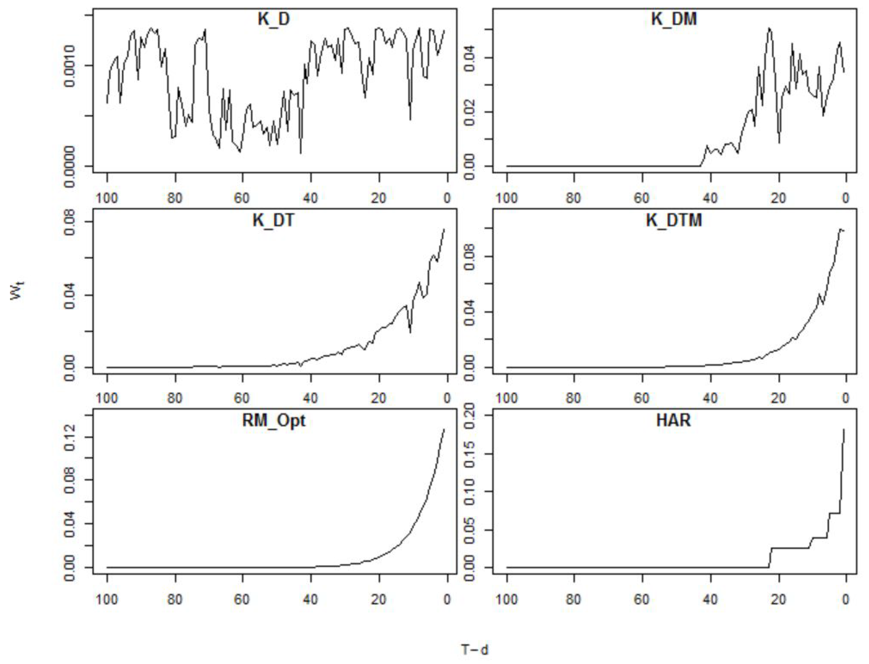
Figure 2.
Histograms of weighted lags, as per Equation (18), for six different forecasting methods during the forecast period. The statistics are calculated from the forecasting models using the RVCM and the recursive sampling scheme.
Figure 2.
Histograms of weighted lags, as per Equation (18), for six different forecasting methods during the forecast period. The statistics are calculated from the forecasting models using the RVCM and the recursive sampling scheme.

Figure 3.
Percentage improvement of the QLIKE/Stein statistics, applied to a hold-out sample (see Section 4.3) when using a variable as the only kernel weighting variable, compared to a simple historical average (equal weights). The evaluation is undertaken for the kernel models using RVCM and a recursive sample scheme. This exercise is repeated every 264 trading days. The results for the variables not represented in this Figure are qualitatively comparable to one of the included variables. Eigenvalue Ratios (Equation (10)) is similar to the included MVQlike; Sign Differences (Equation (12)) is similar to the Temperature in Dubai; Risk Premium and Oil Price are similar to the Yield Spread and VIX and Gold Price are similar to MVQlike.
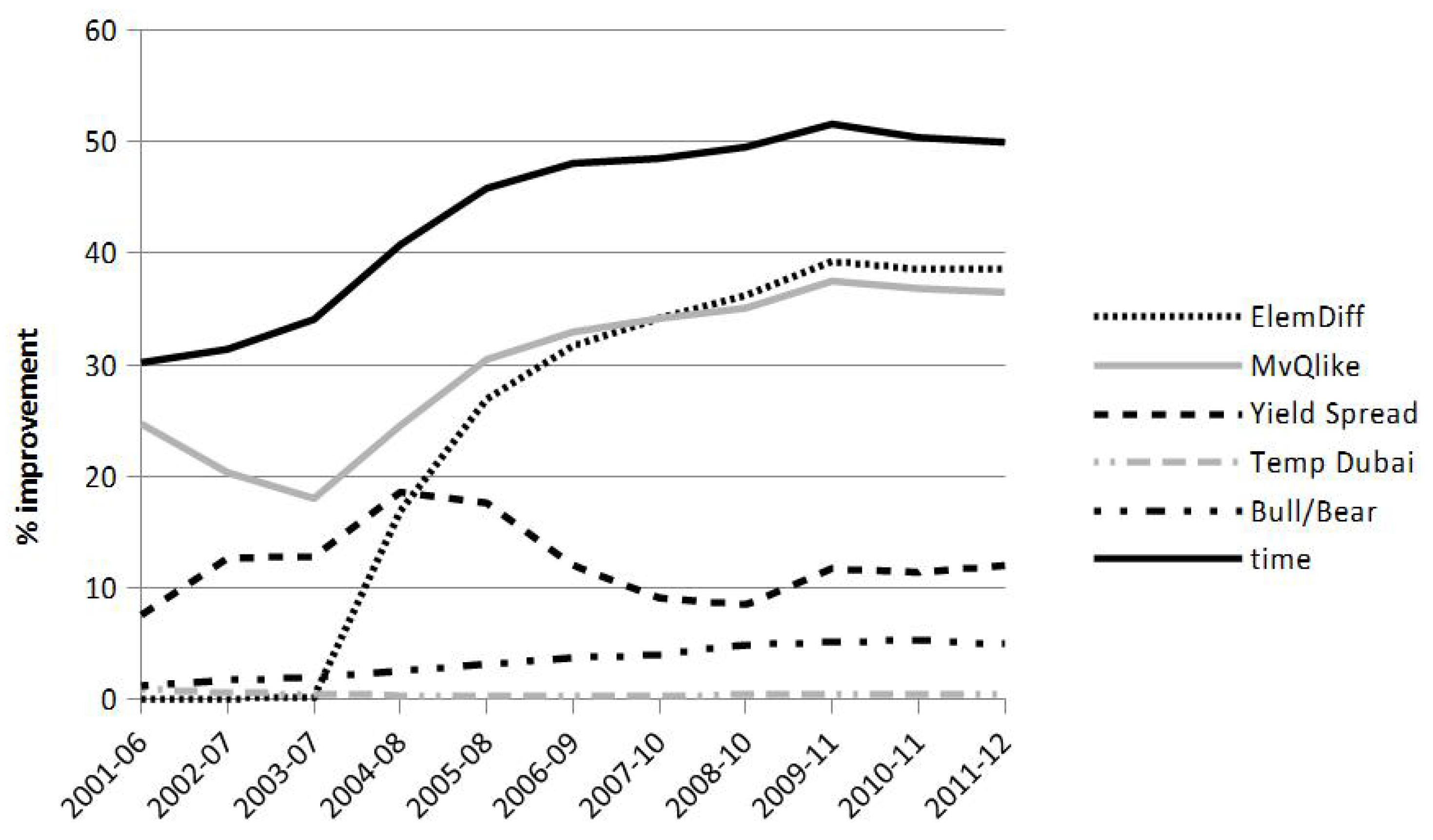
Figure 4.
Graph of for each of the 12 variables across the forecasting period.
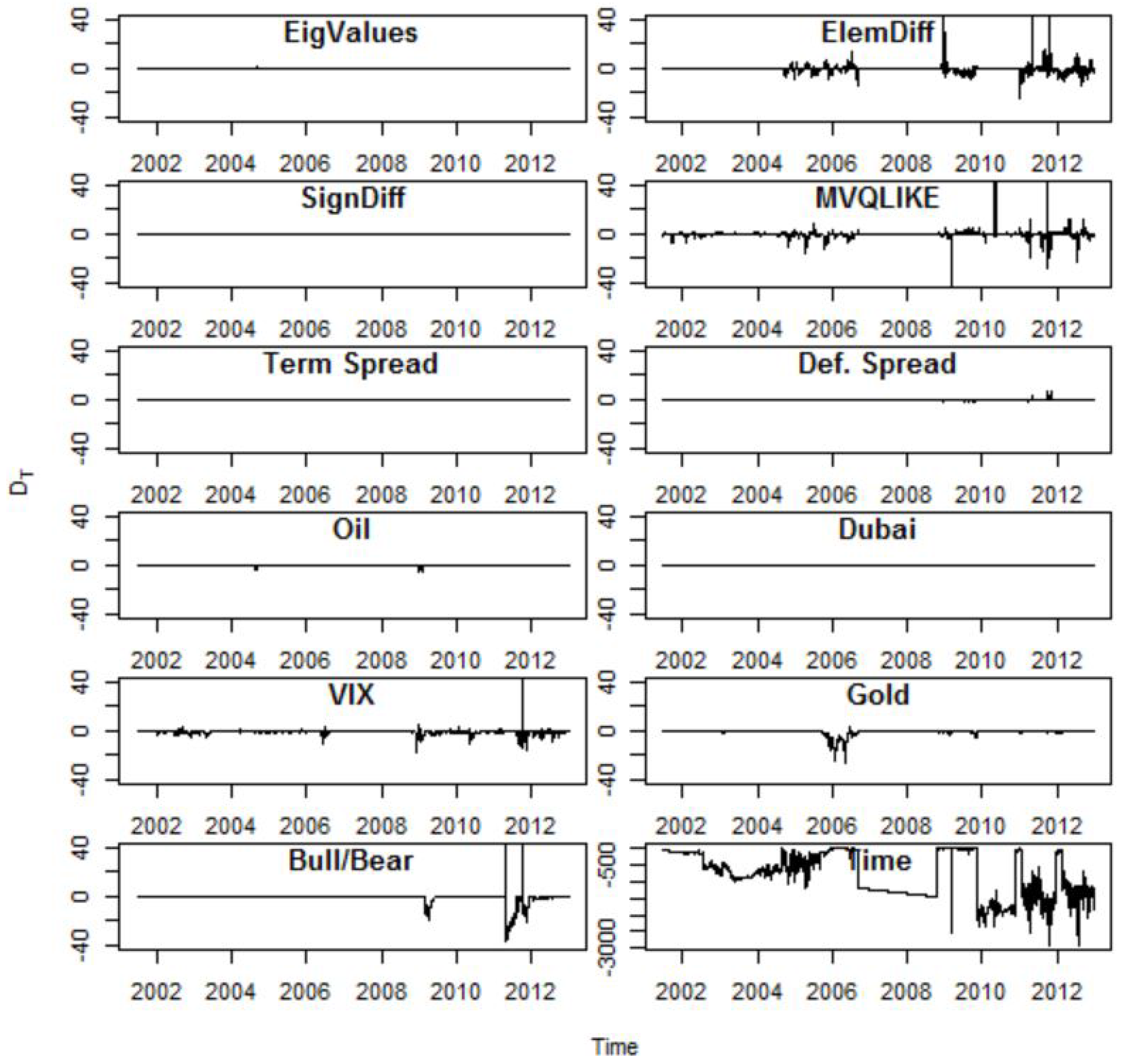
Table 1.
VCM Forecasting Models considered.
| Label | Short Description |
|---|---|
| K_TDM | Kernel forecasting method with time, matrix distance and macroeconomic information as explanatory variables |
| K_DM | Kernel forecasting method with matrix distance and macroeconomic variables |
| K_TD | Kernel forecasting method time and matrix distance variables |
| K_D | Kernel forecasting method which excludes both time and macroeconomic variables and only includes matrix distance measures |
| HAR_CD | HAR Forecasting method using the Cholesky Decomposition |
| HAR_LOG | HAR Forecasting method using the Matrix Logarithm Decomposition |
| RM | Riskmetrics method using pre-defined values for decay |
| RM_Opt | Riskmetrics using an optimised decay parameter |
Table 2.
Model Confidence Set (MCS) p-values for different forecast models. On the basis of 2901 daily 1-day ahead forecasts (19 June 2001 to 31 December 2012). The MCS algorithm is applied to the indicated loss functions. Values larger than 0.05 indicate models that would be included in 95% confidence MCS. is proxied by the realized variance covariance matrix using a regular grid of 5 min intra-day returns. Recursive/Rolling indicates the type of estimation window used. RMVK represents models that used the multivariate kernel estimates to estimate the variance covariance matrix while RVCM indicates that the model used an estimate based on a regular grid of 5 min intra-day returns. Loss functions: (MV)QLIKE as defined in (16); MSE is the mean squared difference between the forecast and observed variance covariance matrix as measured across all elements, , scaled by .
| VCM est | RMVK | RVCM | ||||||
|---|---|---|---|---|---|---|---|---|
| Sampling | Rolling | Recursive | Rolling | Recursive | ||||
| Model | QLIKE | MSE | QLIKE | MSE | QLIKE | MSE | QLIKE | MSE |
| K_D | 1 | 0.538 | 0 | 0.46 | 0.1 | 0.896 | 0 | 0.64 |
| K_DM | 0.02 | 0.538 | 0 | 0.3 | 0.896 | 0.01 | 0 | 0.6 |
| K_TDM | 0.53 | 0.538 | 0.047 | 1 | 0 | 0.896 | 0.022 | 1 |
| K_TD | 0.2 | 1 | 1 | 0.77 | 0 | 0.896 | 1 | 0.64 |
| HAR_CD | 0 | 0.986 | 0 | 0.34 | 0 | 1 | 0 | 0.64 |
| HAR_LOG | 0 | 0.243 | 0 | 0.22 | 0 | 0.297 | 0 | 0.26 |
| RM | 0.06 | 0.177 | 0.005 | 0.15 | 0.01 | 0.156 | 0 | 0.14 |
| RM_Opt | 0.06 | 0.986 | 0 | 0.46 | 1 | 0.896 | 0 | 0.64 |
Table 3.
Results of MCS analysis of 1 day ahead forecasts over two year periods the period 2001–2012. Results in this Table are based on forecasting models that use the RVCM as estimates for the variance covariance model in the forecasting models, and as proxies for , the variance covariance matrix. Sampling method is recursive and the loss function used in the MCS algorithm is the QLIKE loss function.
| 2001–2002 | 2003–2004 | 2005–2006 | 2007–2008 | 2009–2010 | 2011–2012 | |||||||
|---|---|---|---|---|---|---|---|---|---|---|---|---|
| Av. Loss | Pval | Av. Loss | Pval | Av. Loss | Pval | Av. Loss | Pval | Av. Loss | Pval | Av. Loss | Pval | |
| K_DM | 7.4926 | 0.01 | 7.3289 | 0 | 7.6893 | 0.001 | 11.3613 | 0 | 10.6056 | 0 | 9.8433 | 0.016 |
| K_D | 9.6571 | 0 | 10.2559 | 0 | 7.9274 | 0 | 10.7996 | 0.002 | 10.7521 | 0 | 10.2044 | 0 |
| K_TDM | 7.1727 | 1 | 7.1398 | 1 | 7.3832 | 1 | 9.8082 | 0.008 | 9.5993 | 0.118 | 9.3501 | 0.21 |
| K_TD | 7.2663 | 0.158 | 7.2028 | 0.003 | 7.3833 | 0.997 | 9.4967 | 1 | 9.4073 | 1 | 9.1939 | 1 |
| HAR_CD | 8.1583 | 0.009 | 7.3687 | 0 | 7.5808 | 0 | 11.2403 | 0.002 | 11.067 | 0 | 10.3472 | 0 |
| HAR_LOG | 8.6004 | 0 | 7.9947 | 0 | 8.4708 | 0 | 12.1655 | 0 | 11.6134 | 0 | 11.2819 | 0 |
| RM | 8.0545 | 0.01 | 7.1912 | 0.133 | 7.4499 | 0.184 | 10.6856 | 0.008 | 10.0059 | 0.005 | 9.4448 | 0.21 |
| RM_Opt | 7.2539 | 0.158 | 7.2429 | 0 | 7.4573 | 0.001 | 9.8331 | 0.008 | 9.6222 | 0.118 | 9.4153 | 0.016 |
© 2018 by the authors. Licensee MDPI, Basel, Switzerland. This article is an open access article distributed under the terms and conditions of the Creative Commons Attribution (CC BY) license (http://creativecommons.org/licenses/by/4.0/).
Share and Cite
MDPI and ACS Style
Becker, R.; Clements, A.; O'Neill, R. A Multivariate Kernel Approach to Forecasting the Variance Covariance of Stock Market Returns. Econometrics 2018, 6, 7. https://doi.org/10.3390/econometrics6010007
AMA Style
Becker R, Clements A, O'Neill R. A Multivariate Kernel Approach to Forecasting the Variance Covariance of Stock Market Returns. Econometrics. 2018; 6(1):7. https://doi.org/10.3390/econometrics6010007
Chicago/Turabian StyleBecker, Ralf, Adam Clements, and Robert O'Neill. 2018. "A Multivariate Kernel Approach to Forecasting the Variance Covariance of Stock Market Returns" Econometrics 6, no. 1: 7. https://doi.org/10.3390/econometrics6010007
Note that from the first issue of 2016, this journal uses article numbers instead of page numbers. See further details here.