Parametric Inference for Index Functionals

Abstract

In this paper, we study the finite sample accuracy of confidence intervals for index functional built via parametric bootstrap, in the case of inequality indices. To estimate the parameters of the assumed parametric data generating distribution, we propose a Generalized Method of Moment estimator that targets the quantity of interest, namely the considered inequality index. Its primary advantage is that the scale parameter does not need to be estimated to perform parametric bootstrap, since inequality measures are scale invariant. The very good finite sample coverages that are found in a simulation study suggest that this feature provides an advantage over the parametric bootstrap using the maximum likelihood estimator. We also find that overall, a parametric bootstrap provides more accurate inference than its non or semi-parametric counterparts, especially for heavy tailed income distributions.

1. Introduction

In this paper, we consider the problem of inference for an index functional T, i.e., quantities of interest that can be written as a function of the data generating model. Given a sample $x_i,i=1,\dots ,n$ and an associated distribution F such that one can assume that $X_i\sim F,i=1,\dots ,n$, we are interested in computing confidence intervals or proceeding with hypothesis testing for $T(F)$. For that, there exists many different approaches that are based on either $T(F^{(n)})$ or $T(F_{\theta })$, where $F^{(n)}$ is the empirical distribution (hence leading to a nonparametric approach) and $F_{\theta },\theta \in \Theta \subset {\mathrm{I}\mathrm{R}}^p$ is a parametric model for which $\theta$ needs to be estimated from the sample (hence leading to a parametric approach).

As a leading example, we consider T to be an inequality index and F an income distribution. Inequality indices are welfare indices which can be very generally written in the following quasi-additively decomposable form (see Cowell and Victoria-Feser (2002, 2003) for the original formal setting)

$$W_{\mathrm{QAD}}(F)=\int \phi \left(x,\mu (F)\right)dF(x),$$

(1)

where $\phi$ is piecewise differentiable in $\mathrm{I}\mathrm{R}$. The generalized entropy family of inequality indices given by

$$I_{\mathrm{GE}}^{\xi }(F)=\frac{1}{{\xi }^2-\xi }\left[\int {\left[\frac{x}{\mu (F)}\right]}^{\xi }dF(x)-1\right],$$

(2)

is obviously obtained by setting

$$\phi \left(x,\mu (F)\right)=\frac{1}{{\xi }^2-\xi }\left[{\left[\frac{x}{\mu (F)}\right]}^{\xi }-1\right].$$

(3)

For example, the cases $\xi =0$ and $\xi =1$ are given by

$$\begin{array}{ccc}\hfill I_{\mathrm{GE}}^0(F)& =& -\int log\left(\frac{x}{\mu (F)}\right)dF(x),\hfill \\ \hfill I_{\mathrm{GE}}^1(F)& =& \int \frac{x}{\mu (F)}log\left(\frac{x}{\mu (F)}\right)dF(x),\hfill \end{array}$$

(4)

with $I_{\mathrm{GE}}^0(F)$ being the Mean Logarithmic Deviation (see Cowell and Flachaire 2015) and $I_{\mathrm{GE}}^1(F)$ being the Theil index. A notable exception to the class in (1) is the Gini coefficient which can be expressed in several forms, such as

$$I_{\mathrm{Gini}}(F)=1-2{\int }_0^1\frac{C(F;q)}{\mu (F)}dq,$$

(5)

with $C(F;q)={\int }^{F^{-1}(q)}xdF(x)$, the cumulative income functional. Inference on $T(F)$ can be done in several manners:

• The (nonparametric) bootstrap is a distribution-free approach that allows to derive the sample distribution of $T(F^{(n)})$ from which quantiles (for confidence intervals) and variance (for testing) can be estimated; for application to inequality indices, see e.g., Mills and Zandvakili (1997) and Biewen (2002).
• Another distribution-free approach consists in deriving the asymptotic variance of the index using the Influence Function ($IF$) of Hampel (1974) (see also Hampel et al. 1986) as is done in Cowell and Victoria-Feser (2003) (for different types of data features such as censoring and truncating) and estimate it directly from the sample (see also Victoria-Feser 1999; Cowell and Flachaire 2015).
• A parametric (and asymptotic) approach, given a chosen parametric model $F_{\theta }$ for the data generating model, consists in first consistently estimating $\theta$, say $\widehat{\theta }$, then considering its asymptotic properties such as its variance $\mathrm{var}(\widehat{\theta })$ and derive the corresponding asymptotic variance of $T(F_{\widehat{\theta }})$ using e.g., the delta method (based on a first order Taylor series expansion).
• A parametric (finite sample) approach, given a chosen parametric model $F_{\theta }$ for the data generating model, consists in first consistently estimating $\theta$, say $\widehat{\theta }$, then using parametric bootstrap to derive the sample distribution of $T(F_{\widehat{\theta }})$ from which quantiles (for confidence intervals) and variance (for testing) can be estimated.
• Refinements and combinations of these approaches.

While most would agree that the fully parametric and asymptotic approach based on the delta method cannot provide as accurate inference as the other methods, it is not clear that avoiding the specification of a parametric model is the way to go. Indeed, for example, Cowell and Flachaire (2015) notice that nonparametric bootstrap inference on inequality indices is sensitive to the exact nature of the upper tail of the income distribution, in that bootstrap inference is expected to perform reasonably well in moderate and large samples, unless the tails are quite heavy. Similar conclusions are also drawn in Davidson and Flachaire (2007); Cowell and Flachaire (2007); Davidson (2009); Davidson (2010) and Davidson (2012). This has for example motivated Schluter and van Garderen (2009) and Schluter (2012), using the results of Hall (1992), to propose normalizing transformations of inequality measures using Edgeworth expansions, to adjust asymptotic Gaussian approximations.

Alternatively, Davidson and Flachaire (2007) and Cowell and Flachaire (2007) consider a semi-parametric bootstrap, where bootstrap samples are generated from a distribution which combines a parametric estimate of the upper tail, namely the Pareto distribution, with a nonparametric estimate the other part of the distribution. We note that modelling the upper tail with a parametric model is common in instances were not only the interest lies in the upper tail itself but also where the data are sparse. For example, in finance, determination of the value at risk or expected shortfall is central to portfolio management, and in insurance, it is important to estimate probabilities associated with given levels of losses. A critical challenge is then to select the threshold from which the upper tail is modelled parametrically (see for example Danielsson et al. 2001; Guillou and Hall 2001; Beirlant et al. 2002; Dupuis and Victoria-Feser 2006 and the references therein).

Cowell and Flachaire (2015) propose to use a another type of semi-parametric approach by which a mixture of lognormal distributions is first considered and then data are generated from the estimated mixture. A mixture of lognormal distributions to model the data can be thought of as a compromise between fully parametric and nonparametric estimation. The use of mixtures for income distribution estimation can be found for example in Flachaire and Nuñez (2007) and the references in Cowell and Flachaire (2015).

Through a simulation study, Cowell and Flachaire (2015), Table 7, compare the actual coverage probabilities of 95% confidence intervals for the Theil index, using, as data generating models, the lognormal distribution and the Singh-Maddala (SM) distribution (Singh and Maddala 1976), with varying parameters to increase the heaviness of the tail. The different methods cited above are compared. Cowell and Flachaire (2015) conclude that, in the presence of very heavy-tailed distributions, even if significant improvements can be obtained on the fully asymptotic and the standard bootstrap methods, none of the alternative methods provides very good results overall.

Moreover, Cowell and Flachaire (2015) do not consider a parametric bootstrap and this has motivated the present paper. Namely, we study the behaviour of coverage probabilities associate to the index functional $T(F)$ using a parametric bootstrap based on samples generated from $F_{\widehat{\theta }}$ (i.e., Approach 4). A parametric model introduces a form of smoothness into the inferential procedure which can lead to more accurate inference. This is for example a fundamental argument for modelling the upper tail with a Pareto distribution. Specifying a parametric distribution for the data generating process can be considered as an additional risk of introducing “error” in the inferential procedure. With income distributions, common wisdom however suggests that some parametric models are sufficiently flexible to encompass most of the data generating processes observed with real data. For example, the four parameters generalized beta distribution of second kind (GB2) proposed by (McDonald 1984), which encompasses the generalized gamma, the Singh-Maddala and Dagum distribution (Dagum 1977) (see also McDonald and Xu 1995), can be considered as sufficiently general to model income data. If this is not the case, then one would wonder if the lack of flexibility of a general four parameter model is not due to a spurious amount of observations, and hence consider a robust estimation approach as proposed and motivated in Cowell and Victoria-Feser (1996), see also (Cowell and Victoria-Feser 2000).

In this paper, as an alternative to the classical Maximum Likelihood Estimator (MLE), we propose a Target Matching Estimator (TME), a member of the class of Generalized Method of Moments (GMM) estimators (Hansen 1982), where one of the “moments” is the targeted inequality index T. It has the advantage that for inference on T, the scale parameter does not need to be estimated (and hence can be set to an arbitrary value), so that the estimation exercise is simpler in that the optimization is performed in a smaller dimension. We derive its asymptotic properties and compare them to the MLE when targeting $T(F_{\theta })$. As illustrated in a simulation study, it turns out that the finite sample coverage probabilities obtained from a parametric bootstrap based on this alternative estimator are far more accurate than the ones computed with other methods, especially with heavy tailed income distributions.

2. A Target Matching Estimator

Recall that we are interested in making inference on an inequality index T and we assume that the sample data are generated from a (sufficiently general) parametric mode $F_{\theta }$, $\theta \in \Theta \subset {\mathrm{I}\mathrm{R}}^p$. We let $\nu ={(T,S_1,\cdots ,S_{q-1})}^{\prime }$ be a vector of statistics of length q, where the first element is the statistic of interest and the remaining $q-1$ elements are additional statistics. We denote by $\widehat{\nu }$ the sample vector of statistics and by ${\nu }_n(\theta )$ its expectation at the model $F_{\theta }$, for a fixed sample size n. Assuming that the mapping $\theta \mapsto {\nu }_n(\theta )$ is bijective, a GMM estimator can be defined as

$$\widehat{\theta }=\underset{\theta \in \Theta }{argmin}{∥\widehat{\nu }-{\nu }_n(\theta )∥}_{\Omega }^2$$

(6)

where $\Omega$ is positive definite $q\times q$ matrix of weights, possibly estimated from the sample (in that case one assumes that it converges to a non-stochastic quantity), used to adjust the statistical efficiency of $\widehat{\theta }$. If ${\nu }_n(\theta )$ cannot be obtained in an analytically tractable form, one can use instead $\nu (\theta )={lim}_{n\to \infty }{\nu }_n(\theta )$, or alternatively, use Monte Carlo simulations to approximate ${\nu }_n(\theta )$, leading to a Simulated Method of Moments (SMM) estimator (McFadden 1989) given by

$$\widehat{\theta }=\underset{\theta \in \Theta }{argmin}{∥\widehat{\nu }-{\overline{\nu }}_n(\theta )∥}_{\Omega }^2$$

(7)

where ${\overline{\nu }}_n(\theta )=\frac{1}{B}{\sum }_{b=1}^B{\widehat{\nu }}_b$ and ${\widehat{\nu }}_b={\widehat{\nu }}_b(F_{\theta })$ is the b-th vector of statistics obtained on pseudo-values simulated from $F_{\theta }$. If the number of simulation B is infinite, then the estimators in (6) and (7) are equivalent, otherwise the latter is (asymptotically) less efficient.

It is computationally advantageous to have an analytic expression for $\nu (\theta )$ and thus prefer this approximation over ${\overline{\nu }}_n(\theta )$. However, in finite samples, the bias on $\widehat{\theta }$ using $\nu (\theta )$ may be more important than the one resulting from using ${\overline{\nu }}_n(\theta )$ (see Guerrier et al. 2018). An other approach, considered for example by Arvanitis and Demos (2015), is to directly approximate ${\nu }_n(\theta )$ with expansions on analytical functions.

Given that the interest here is to make inference about a functional T, one also needs to consider a suitable choice for the (additional) statistics in $\nu$. Obviously one needs to choose a number of statistics at least as large as the number of parameter in the assumed model, i.e., $q\ge p$. If these statistics are sufficient, then $q=p$. Moreover, T may depend only on $q_s<p$ of the elements of $\theta$, and for this purpose, the whole estimation of $\theta$ maybe an unnecessary burden. Let $\theta ={({{\theta }^s}^{\prime },{{\theta }^c}^{\prime })}^{\prime }$ where ${\theta }^s$, of dimension $q_s\ge 1$ is the vector of parameters that (uniquely) determines T whereas ${\theta }^c$, of dimension $q_c$, is the vector of “nuisance parameters” that do not influence T. Then, instead of solving (6) or (7), we propose to consider a Target Matching Estimator (TME) defined as

$${\widehat{\theta }}^s=\underset{{\theta }^s\in {\Theta }^s\subset {\mathrm{I}\mathrm{R}}^{q_s}}{argmin}{∥{\widehat{\nu }}^s-\nu ({\theta }^s)∥}_{\Sigma }^2.$$

(8)

It is known that in an homogeneous system the asymptotic covariance of ${\widehat{\theta }}^s$ is not influenced by the weighting matrix $\Sigma$ (supposedly independent from $\theta$) as long as $\Sigma$ is a positive-definite matrix. Since we consider the case when the dimension of the statistics and the parameters of interest are the same, i.e., $dim(\nu )=dim({\theta }^s)=q^s$, taking the identity matrix for $\Sigma$, and assuming that the minimum of the quadratic function is attained in the interior of the parameter space ${\Theta }^s$, we then have that (8) can be equivalently written as

$${\widehat{\theta }}^s=\underset{{\theta }^s\in {\Theta }^s\subset {\mathrm{I}\mathrm{R}}^{q_s}}{argzero}\left[{\widehat{\nu }}^s-\nu ({\theta }^s)\right].$$

The generalized entropy family of measures and the Gini index are scale invariant whereas the models $F_{\theta }$ usually suggested in the literature (Kleiber and Kotz 2003) are parametrised with a scale component. Indeed, let $\delta$, an element of $\theta$, denote the scale parameter, then with the linear property of the expectation, $I_{\mathrm{GE}}^{\xi }(F)$ in (2) is invariant to any transformation $\delta X$. The same statement is true for the Gini coefficient. This is not surprising as scale-invariance is indeed one of the required property of inequality indices. We hence have $(\partial /\partial \delta )T(F_{\theta })=0$, so that ${\theta }^s$ is $\theta$ without the scale parameter $\delta$. Note that $(\partial /\partial \delta )T(F_{\theta })=0$ may be useful in situations where the analytical form of $T(F_{\theta })$ is not available.

More generally, suppose we are in the situation where T is such that $(\partial /\partial {\theta }^c)T(F_{\theta })=0$ and $(\partial /\partial {\theta }^s)T(F_{\theta })\ne 0$. Also suppose that the statistics $S_1,\cdots ,S_{q-1}$ are chosen such that $(\partial /\partial {\theta }^c)S_j(F_{\theta })=0$ and $(\partial /\partial {\theta }^s)S_j(F_{\theta })\ne 0$, $j=1,\dots ,q-1$, $q=p$, then (8) provides a suitable estimator for inference on T. For scale invariant inequality measures T, any statistics of the form

$$S_k(x)=\frac{1}{n}\sum _{i=1}^n{\left(\frac{x_i}{\widehat{\mu }}\right)}^k,k\in \mathrm{I}\mathrm{R},\widehat{\mu }=\frac{1}{n}\sum _{i=1}^n{x}_i,$$

(9)

is also scale-invariant. This is also true with a logarithmic transformation as

$$U_l(x)=\frac{1}{n}\sum _{i=1}^n{(log(x_i)-\widehat{m})}^l,l\in \mathrm{I}\mathrm{R},\widehat{m}=\frac{1}{n}\sum _{i=1}^{n}log(x_i).$$

(10)

Finally, for the choice of $F_{\theta }$, one can consider the GB2 (see Section 4) which is sufficiently general to encompass real data situations with income data (Bandourian et al. 2002). Alternatively, as suggested for example in Cowell and Flachaire (2015), one can also consider the SM distribution.

In the simulation Section 4 we propose suitable statistics $\nu$ that are used in (8). Given these statistics $\nu$ and an assumed data generating model $F_{\theta }$, inference about T, using the parametric bootstrap, is obtained using Algorithm 1.

Algorithm 1: TME-percentile confidence interval

Note that if $\overline{\nu }({\theta }^s)$ is used instead of $\nu ({\theta }^s)$ in (8), the last step of the optimization leading to ${\widehat{\theta }}^s$ readily delivers $(T_1,\cdots ,T_B)$.

3. Asymptotic Properties

We now look at the asymptotic distribution of the TME in (8). Since ${\theta }^c$ is fixed but ${\theta }^s$ is estimated by matching some statistics $\nu$, a crucial question is on whether ${\widehat{\theta }}^s$ is more efficient than say ${\widehat{\theta }}_{\mathrm{MLE}}^s$, the estimator that we would have obtained by the MLE on the whole vector $\theta$. In order to answer this question consider a setting in which the regular conditions for the MLE ${\widehat{\theta }}_{\mathrm{MLE}}$ to be square root-n consistent are met. In this case, we let $\mathcal{I}$ denotes the Fisher information matrix evaluated at the point ${\theta }_0\in \Theta$, we have

$$n^{1/2}\left({\widehat{\theta }}_{\mathrm{MLE}}-{\theta }_0\right)⇝\mathcal{N}\left(0,{\mathcal{I}}^{-1}\right).$$

This setting is clearly not the weakest possible in theory for our analysis and may be further relaxed. We do not attempt to pursue the weakest possible conditions to avoid overly technical treatments in establishing the theoretical result given in this section.

Theorem 1.

Let ${\Theta }^s\subset {\mathrm{I}\mathrm{R}}^{q_s}$ be compact. Suppose that the point ${\theta }_0^s$ is in the interior of ${\Theta }^s$. Suppose that $\nu ({\theta }_0^s)$ is the expectation of ${\widehat{\nu }}^s$ when n is large. If $n^{1/2}\left({\widehat{\nu }}^s-\nu ({\theta }_0^s)\right)$ satisfies a central limit theorem with covariance matrix Ξ, the mapping $\theta \mapsto \nu$ is bijective, continuously once differentiable in an open neighborhood of the point ${\theta }_0^s\in {\Theta }^s$ and the derivative $\dot{\nu }$ is nonsingular at the point ${\theta }_0^s$, then

$$n^{1/2}\dot{\nu }({\theta }_0^s)\left({\widehat{\theta }}^s-{\theta }_0^s\right)⇝\mathcal{N}\left(0,\mathrm{\Xi }\right).$$

The proof is provided in the Appendix A.

Compared to the MLE, the additional condition that the statistics ${\widehat{\nu }}^s$ satisfy a central limit theorem is mild and generally met in practice for sample moments and the inequality indices considered here. The results on the delta method and the continuous mapping theorem of Phillips (2012) may be employed to refine Theorem 1 to the case where the known function $\nu$ is replaced by the function evaluated by simulation ${\overline{\nu }}_n$.

The asymptotic covariance matrix of ${\widehat{\theta }}^s$, given in Theorem 1 by ${[\dot{\nu }{({\theta }_0^s)}^{\prime }]}^{-1}\mathrm{\Xi }\dot{\nu }{({\theta }_0^s)}^{-1}$, is proportional to the inverse of the derivative of the expectation of the statistics with respect to $\theta$ and the asymptotic covariance matrix of the statistics. The choice of statistics should then be guided by their sensitivity to $\theta$ and their variability at the model. The same argument is found in Heggland and Frigessi (2004).

If the statistics $\nu$ are sufficient, then the asymptotic covariance matrix of ${\widehat{\theta }}^s$ is equivalent to the asymptotic covariance matrix of the MLE conditionally on ${\widehat{\theta }}_{\mathrm{MLE}}^c$ fixed. From the properties of the normal distribution, we have asymptotically that

$$n^{1/2}\left({\widehat{\theta }}_{\mathrm{MLE}}^s-{\theta }_0^s\right)|\left({\widehat{\theta }}_{\mathrm{MLE}}^c={\theta }_0^c\right)⇝\mathcal{N}\left(\mathbf{0},V_{ss}\right),$$

where $V_{ss}={\mathcal{I}}_{ss}^{-1}-{[{\mathcal{I}}^{-1}]}_{sc}{\mathcal{I}}_{cc}{[{\mathcal{I}}^{-1}]}_{cs}$, ${\mathcal{I}}_{ss}$ denotes the partition of $\mathcal{I}$ corresponding to ${\theta }^s$, ${\mathcal{I}}_{cc}$ for ${\theta }^c$ and ${[{\mathcal{I}}^{-1}]}_{sc}$ for the covariances between ${\widehat{\theta }}_{\mathrm{MLE}}^s$ and ${\widehat{\theta }}_{\mathrm{MLE}}^c$. Thus, the estimator ${\widehat{\theta }}^s$ obtained from (8) has a smaller variance than the unconditional MLE by a factor ${[{\mathcal{I}}^{-1}]}_{sc}{\mathcal{I}}_{cc}{[{\mathcal{I}}^{-1}]}_{cs}\ge 0$. In particular, this gain could by substantial if ${\widehat{\theta }}^c$ has a large variance. On the other hand, the gain would be null if ${\widehat{\theta }}^s$ and ${\widehat{\theta }}^c$ are independent as their covariances ${[{\mathcal{I}}^{-1}]}_{sc}={[{\mathcal{I}}^{-1}]}_{cs}^{\prime }=0$.

Choosing “good” statistics ${\widehat{\nu }}^s$ remains a difficult task: sufficient statistics with appropriate data reduction and with the property of being independent (asymptotically) from ${\theta }^c$ may be hard to find. Heggland and Frigessi (2004) suggest a graphical procedure based on simulation to find statistics “sensitive enough” to the parameter of interest. In a similar context, Gallant and Tauchen (1996) propose to use the likelihood score function of a model “close” to the one of interest as statistics. In the present context, it could be a probability model parametrised by ${\theta }^s$ only. There are however no guarantee that such a model exists, and if it does, it might be not unique.

4. Simulation Study

We consider here two parametric distributions, namely the four parameters GB2 and the three parameters SM distributions. We compare the coverage probabilities provided by the parametric bootstrap using on the one hand the MLE and on the other hand the TME approach presented in Section 2 (using Algorithm 1) to the nonparametric bootstrap for the GB2. We also compare the coverage probabilities assuming a SM data generating process, to a variance stabilizing transform of the index proposed by Schluter (2012) (Varstab), the semi-parametric approach of Davidson and Flachaire (2007) and Cowell and Flachaire (2007) (Semip) and when mixtures of lognormal distributions are used to fit the density as proposed in Cowell and Flachaire (2015).

The GB2 has density function

$$f_{\theta }(x)=\frac{a{x}^{ap-1}}{b^{ap}\mathcal{B}(p,q){(1+{(x/b)}^a)}^{p+q}},x,a,b,p,q>0,$$

(11)

where $\mathcal{B}$ is the beta function, b is the scale parameter, a, p and q are shape parameters. Note that here we consider a to be positive, yet, the distribution of the inverse may be obtained by allowing a to be negative (McDonald and Xu 1995). Suppose we are interested in the Theil index defined in (4), the population index, with $\theta ={(a,b,p,q)}^{\prime }$, is given by

$$\begin{array}{cc}\hfill T(F_{\theta })=& log(\Gamma (p))+log(\Gamma (q))-log\left(\Gamma \left(\frac{aq-1}{a}\right)\right)-log\left(\Gamma \left(\frac{ap+1}{a}\right)\right)\hfill \\ & +\frac{1}{a}\left[\psi \left(\frac{ap+1}{a}\right)-\psi \left(\frac{aq-1}{a}\right)\right],\hfill \end{array}$$

where $\Gamma$ is the gamma function and $\psi$ is the digamma function. Clearly the Theil index is scale invariant, so that we set ${\theta }^s={(a,p,q)}^{\prime }$ and ${\theta }^c=b$.

The population values of the statistics $S_k$ in (9) are given by

$$S_k(F_{\theta })=\frac{{\left[\Gamma (p)\Gamma (q)\right]}^{k-1}\Gamma \left(\frac{aq-k}{a}\right)\Gamma \left(\frac{ap+k}{a}\right)}{{\left[\Gamma \left(\frac{aq-1}{a}\right)\Gamma \left(\frac{ap+1}{a}\right)\right]}^k},k\in \mathrm{I}\mathrm{R},$$

and the ones for $U_l$ in (10), for $l=2,3$, are given by

$$\begin{array}{cc}\hfill U_2(F_{\theta })& =\frac{{\psi }^{(1)}(p)+{\psi }^{(1)}(q)}{a^2},\hfill \\ \hfill U_3(F_{\theta })& =\frac{{\psi }^{(2)}(p)-{\psi }^{(2)}(q)}{a^3},\hfill \end{array}$$

where ${\psi }^{(m)}$ is the polygamma function, i.e., the m-th derivative of the digamma function $\psi$.

As is done in Cowell and Flachaire (2015), we consider the SM distribution with density

$$f_{\theta }(x)=\frac{aq{x}^{a-1}}{b^a{(1+{(x/b)}^a)}^{1+q}},x,a,b,q>0,$$

(12)

and corresponding population statistics T, $S_k$ and $U_l$, $l=2,3$, given by

$$\begin{array}{cc}\hfill T(F_{\theta })=& 1+log(\Gamma (q))-log\left(\Gamma \left(\frac{aq-1}{a}\right)\right)-log\left(\Gamma \left(\frac{a+1}{a}\right)\right)\hfill \\ & +\frac{1}{a}\left[\psi \left(\frac{1}{a}\right)-\psi \left(\frac{aq-1}{a}\right)\right],\hfill \\ \hfill S_k(F_{\theta })=& \frac{a^k\Gamma {(q)}^{k-1}\Gamma \left(\frac{aq-k}{a}\right)\Gamma \left(\frac{k+a}{a}\right)}{\Gamma \left(\frac{1}{a}\right)\Gamma \left(\frac{aq-1}{a}\right)},k\in \mathrm{I}\mathrm{R},\hfill \\ \hfill U_2(F_{\theta })=& \frac{{\pi }^2+6{\psi }^{(1)}(q)}{6a^2},\hfill \\ \hfill U_3(F_{\theta })=& \frac{-{\psi }^{(2)}(q)-2\zeta (3)}{a^3},\hfill \end{array}$$

where $\zeta (3)$ is the Apéry’s constant.

Under the GB2, for generating the data, we set ${\theta }^s={(a=3,p=3.5,q=0.8)}^{\prime }$, ${\theta }^c=(b=10)$ and $n=250,500,1000$. For the TME, we choose the vector of statistics to be $\nu ={[T(x),U_2(x),U_3(x)]}^{\prime }$ with $T(x)$ the Theil index and $U_j(x),j=2,3$ given in (10). We fix the value of the scale parameter to the arbitrary value of one ($b=1$) in Algorithm 1. We repeat the experiment ${10}^4$ times and set the number of bootstrap replicates to $B={10}^3$.

To solve for ${\widehat{\theta }}^s$ in (8) or for the MLE, we use the classical quasi-Newton optimization algorithm with starting values obtained from the differential evolution heuristic (Storn and Price 1997), in order to mimic a real situation in which the true parameter’s values are unknown.

In

Table 1. Finite sample coverage probability with respect to a nominal confidence level (two-sided) of 95% for the Theil Index. Data are simulated under the GB2 with ${\theta }^s={(a=3,p=3.5,q=0.8)}^{\prime }$, ${\theta }^c=(b=10)$. $\nu ={[T(x),U_2(x),U_3(x)]}^{\prime }$ with $T(x)$ the Theil index. In Algorithm 1, $b=1$. The experiment is repeated ${10}^4$ times and $B={10}^3$.

Sample Size	Boot	MLE	TME
$n=250$	0.708	0.962	0.927
$n=500$	0.753	0.978	0.942
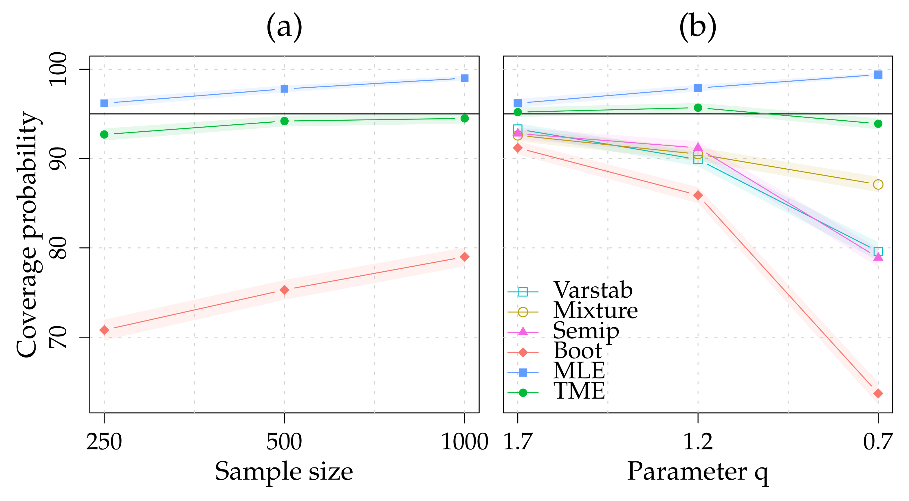
$n=1000$	0.790	0.990	0.949

, we report the performances of the three approaches with respect to a nominal confidence level of 95% for the three sample sizes. As already shown in the literature (see e.g., Cowell and Flachaire 2015), we find poor performance for the nonparametric bootstrap (Boot), far from the nominal confidence level. The parametric bootstrap using the MLE provides reasonable finite sample coverage that are nevertheless conservatives. On the other hand, the performance of parametric bootstrap using the TME is overall satisfactory, with enhanced performance when sample size increases.

In

Table 2. Finite sample coverage probability with respect to a nominal confidence level (two-sided) of 95% for the Theil Index. The values for Varstab, Semip and Mixture are directly reported from (Cowell and Flachaire 2015, Table 6.6). Data are simulated under the Singh-Madalla with $n=500$, ${\theta }^s=(a=2.8,q)$, ${\theta }^c=(b=0.193)$. The parameter q accounts for the shape of the upper tail of the distribution, the smaller the heavier the tail. $\nu ={[T(x),U_2(x)]}^{\prime }$ with $T(x)$ the Theil index. In Algorithm 1, $b=1$. The experiment is repeated ${10}^4$ times and $B={10}^3$.

Singh-Madalla	Varstab	Semip	Mixture	Boot	MLE	TME
$q=1.7$	0.933	0.926	0.928	0.912	0.962	0.952
$q=1.2$	0.899	0.905	0.912	0.859	0.979	0.957
$q=0.7$	0.796	0.871	0.789	0.637	0.994	0.939

, we replicate the simulation study in (Cowell and Flachaire 2015, Table 6.6), and report the values for Varstab, Semip and Mixture. We have ${\theta }^s={(a=2.8,q)}^{\prime }$, ${\theta }^c=(b=0.193)$ and set $\nu ={[T(x),U_2(x)]}^{\prime }$ with $T(x)$ the Theil index and $U_2(x)$ given in (10). We fix the value of the scale parameter to the arbitrary value of one ($b=1$) in Algorithm 1. We repeat the experiment ${10}^4$ times and set the number of bootstrap replicates to $B={10}^3$. The results reported in Table 2 are also presented graphically in Figure 1. Both parametric approaches present finite sample coverage probabilities that are far more accurate than the other approaches, especially in the heavy tail case. As with the GB2, the parametric bootstrap based on the MLE tends to provide conservative coverage probabilities.

5. Conclusions

In this paper, we study the finite sample accuracy of confidence intervals built via parametric bootstrap. We also propose a GMM estimator, the TME, that targets the quantity of interest, namely the considered inequality index. Its primary advantage is that the scale parameter of the assumed parametric model does not need to be estimated to perform parametric bootstrap, since inequality measures are scale invariant. The theoretical result and the simulation study suggest that this feature provides an advantage over the parametric bootstrap using the MLE and also over other established simulation-based inferential methods.

As noted by an anonymous referee, an important point that has not been directly assessed is the specification robustness, i.e., the properties of the proposed method when the assumed general model is not the exact one. This point deserves more (formal) investigation that we leave for further research.

On the more practical side, although this study is limited to two income distributions and one inequality index, the methodology presented here can be extended to other settings in a relative straightforward manner. For example, it is possible to extend the TME to include trimmed inequality indices since it suffices to use the trimmed version of T in $\nu$. If trimming is done for robustness purposes as proposed in Cowell and Victoria-Feser (2003), then the other statistics in $\widehat{\nu }$ should also be robust (see also Victoria-Feser 2000). This is the case, for example, with trimmed moments.

References

- Arvanitis, Stelios, and Antonis Demos. 2015. A class of indirect inference estimators: Higher-order asymptotics and approximate bias correction. The Econometrics Journal 18: 200–41. [Google Scholar] [CrossRef]
- Bandourian, Ripsy, James McDonald, and Robert S. Turley. 2002. A Comparison of Parametric Models of Income Distribution Across Countries and over Time. Available online: http://www.lisdatacenter.org/wps/liswps/305.pdf (accessed on 28 November 2017).
- Beirlant, Jan, Goedele Dierckx, A. Guillou, and Catalin Stărică. 2002. On exponential representations of log-spacings of extreme order statistics. Extremes 5: 157–80. [Google Scholar] [CrossRef]
- Biewen, Martin. 2002. Bootstrap inference for inequality, mobility and poverty measurement. Journal of Econometrics 108: 317–42. [Google Scholar] [CrossRef]
- Cowell, Frank A., and Emmanuel Flachaire. 2007. Income distribution and inequality measurement: The problem of extreme values. Journal of Econometrics 141: 1044–72. [Google Scholar] [CrossRef] [Green Version]
- Cowell, Frank A., and Emmanuel Flachaire. 2015. Statistical Methods for Distributional Analysis. In Handbook of Income Distribution. Edited by François Bourguignon and Anthony B. Atkinson. Amsterdam: Elsevier, vol. 2, pp. 359–465. [Google Scholar]
- Cowell, Frank A., and Maria-Pia Victoria-Feser. 1996. Robustness properties of inequality measures. Econometrica 64: 77–101. [Google Scholar] [CrossRef]
- Cowell, Frank A., and Maria-Pia Victoria-Feser. 2000. Distributional analysis: A robust approach. In Putting Economics to Work, Volume in Honour of Michio Morishima. Edited by Anthony Atkinson, Howard Glennerster and Nicholas Stern. London: STICERD. [Google Scholar]
- Cowell, Frank A., and Maria-Pia Victoria-Feser. 2002. Welfare rankings in the presence of contaminated data. Econometrica 70: 1221–33. [Google Scholar] [CrossRef]
- Cowell, Frank A., and Maria-Pia Victoria-Feser. 2003. Distribution-free inference for welfare indices under complete and incomplete information. Journal of Economic Inequality 1: 191–219. [Google Scholar] [CrossRef]
- Dagum, Camilo. 1977. A new model of personal income distribution: Specification and estimation. Economie Appliquée 30: 413–36. [Google Scholar]
- Danielsson, Jon, Lauredns de Haan, Liang Peng, and Casper G. de Vries. 2001. Using a bootstrap method to choose sample fraction in Tail index estimation. Journal of Multivariate Analysis 76: 226–48. [Google Scholar] [CrossRef]
- Davidson, Russell. 2009. Reliable inference for the Gini index. Journal of Econometrics 150: 30–40. [Google Scholar] [CrossRef]
- Davidson, Russell. 2010. Innis lecture: Inference on income distributions. Canadian Journal of Economics 43: 1122–48. [Google Scholar] [CrossRef]
- Davidson, Russell. 2012. Statistical inference in the presence of heavy tails. Econometrics Journal 15: 31–53. [Google Scholar] [CrossRef]
- Davidson, Russell, and Emmanuel Flachaire. 2007. Asymptotic and bootstrap inference for inequality and poverty measures. Journal of Econometrics 141: 141–66. [Google Scholar] [CrossRef] [Green Version]
- Dupuis, Debbie J., and Maria-Pia Victoria-Feser. 2006. A robust prediction error criterion for Pareto modeling of upper tails. Canadian Journal of Statistics 34: 639–58. [Google Scholar] [CrossRef]
- Flachaire, Emmanuel, and Olivier G. Nuñez. 2007. Estimation of income distribution and detection of subpopulations: An explanatory model. Computational Statistics & Data Analysis 51: 3368–80. [Google Scholar]
- Gallant, A. Ronald, and George Tauchen. 1996. Which moments to match? Econometric Theory 12: 657–81. [Google Scholar] [CrossRef]
- Guerrier, Stephane, Elise Dupuis, Yanyuan Ma, and Maria-Pia Victoria-Feser. 2018. Simulation based bias correction methods for complex models. Journal of the American Statistical Association (Theory & Methods). in press. [Google Scholar] [CrossRef]
- Guillou, Armelle, and Peter Hall. 2001. A diagnostic for selecting the threshold in extreme-value analysis. Journal of the Royal Statistical Society, Series B 63: 293–305. [Google Scholar] [CrossRef]
- Hall, Peter. 1992. The Bootstrap and Edgeworth Expansions. New York: Springer Verlag. [Google Scholar]
- Hampel, Frank R. 1974. The influence curve and its role in robust estimation. Journal of the American Statistical Association 69: 383–93. [Google Scholar] [CrossRef]
- Hampel, Frank R., Elvezio M. Ronchetti, Peter J. Rousseeuw, and Werner A. Stahel. 1986. Robust Statistics: The Approach Based on Influence Functions. New York: John Wiley. [Google Scholar]
- Hansen, Lars Peter. 1982. Large sample properties of generalized method of moments estimators. Econometrica 50: 1029–54. [Google Scholar] [CrossRef]
- Heggland, Knut, and Arnoldo Frigessi. 2004. Estimating functions in indirect inference. Journal of the Royal Statistical Society: Series B (Statistical Methodology) 66: 447–62. [Google Scholar] [CrossRef]
- Kleiber, Christian, and Samuel Kotz. 2003. Statistical Size Distributions in Economics and Actuarial Sciences. New York: John Wiley & Sons, vol. 470. [Google Scholar]
- McDonald, James B. 1984. Some generalized functions for the size distribution of income. Econometrica 52: 647–64. [Google Scholar] [CrossRef]
- McDonald, James B., and Yexiao J. Xu. 1995. A generalization of the beta distribution with applications. Journal of Econometrics 66: 133–52. [Google Scholar] [CrossRef]
- McFadden, Daniel. 1989. Method of simulated moments for estimation of discrete response models without numerical integration. Econometrica 57: 995–1026. [Google Scholar] [CrossRef]
- Mills, Jeffrey A., and Sourushe Zandvakili. 1997. Statistical inference via bootstrapping for measures of inequality. Journal of Applied Econometrics 12: 133–50. [Google Scholar] [CrossRef]
- Newey, Whitney K., and Daniel McFadden. 1994. Large sample estimation and hypothesis testing. In Handbook of Econometrics. Amsterdam: Elsevier, vol. 4, pp. 2111–245. [Google Scholar]
- Phillips, Peter C. B. 2012. Folklore theorems, implicit maps, and indirect inference. Econometrica 80: 425–54. [Google Scholar]
- Rudin, Walter. 1976. Principles of Mathematical Analysis (International Series in Pure & Applied Mathematics). New York: McGraw-Hill Education. [Google Scholar]
- Schluter, Christian. 2012. On the problem of inference for inequality measures for heavy-tailed distributions. The Econometrics Journal 15: 125–53. [Google Scholar] [CrossRef]
- Schluter, Christian, and Kees Jan van Garderen. 2009. Edgeworth expansions and normalizing transforms for inequality measures. Journal of Econometrics 150: 16–29. [Google Scholar] [CrossRef]
- Singh, S. K., and G. S. Maddala. 1976. A function for the size distribution of income. Econometrica 44: 963–70. [Google Scholar] [CrossRef]
- Storn, Rainer, and Kenneth Price. 1997. Differential evolution—A simple and efficient heuristic for global optimization over continuous spaces. Journal of Global Optimization 11: 341–59. [Google Scholar] [CrossRef]
- Van der Vaart, Aad W. 1998. Asymptotic Statistics. Cambridge: Cambridge University Press, vol. 3. [Google Scholar]
- Victoria-Feser, Maria-Pia. 1999. Comment on Giorgi’s chapter: The sampling properties of inequality indices. In Income Inequality Measurement: From Theory to Practice. Edited by J. Silber. Boston: Kluwer Academic Publisher, pp. 260–67. [Google Scholar]
- Victoria-Feser, Maria-Pia. 2000. A general robust approach to the analysis of income distribution, inequality and poverty. International Statistical Review 68: 277–93. [Google Scholar] [CrossRef]
Figure 1.
Illustration of the coverage probabilities obtained over 10,000 Monte Carlo experiments for the GB2 (a) (see Table 1) and the Singh-Madalla (b) (see Table 2). Each color represents a different method. The shade area around each line is the 99.9% asymptotic confidence interval for proportion. The black line is the nominal confidence level of 95%.