Forecasting Inflation Uncertainty in the G7 Countries

1
Department of Economics (CQE), Westfälische Wilhelms-Universität Münster, Am Stadtgraben 9, 48143 Münster, Germany
2
Department of Accounting and Finance, Athens University of Economics and Business, Trias 2, GR 11362 Athens, Greece
3
Department of Economics, European University Institute, Via delle Fontanelle 18, I-50014 Florence, Italy
*
Author to whom correspondence should be addressed.
Econometrics 2018, 6(2), 23; https://doi.org/10.3390/econometrics6020023
Submission received: 16 February 2018
/
Revised: 22 February 2018
/
Accepted: 16 April 2018
/
Published: 27 April 2018
(This article belongs to the Special Issue Recent Developments in Macro-Econometric Modeling: Theory and Applications)
Abstract
:There is substantial evidence that inflation rates are characterized by long memory and nonlinearities. In this paper, we introduce a long-memory Smooth Transition AutoRegressive Fractionally Integrated Moving Average-Markov Switching Multifractal specification [-] for modeling and forecasting inflation uncertainty. We first provide the statistical properties of the process and investigate the finite sample properties of the maximum likelihood estimators through simulation. Second, we evaluate the out-of-sample forecast performance of the model in forecasting inflation uncertainty in the G7 countries. Our empirical analysis demonstrates the superiority of the new model over the alternative --type models in forecasting inflation uncertainty.
JEL Classification:
C22; E311. Introduction
The financial crisis of 2007–2009 and the long-lasting economic recovery has renewed the interest in studying and measuring inflation uncertainty. Studies by Baker et al. (2015) and Jurado et al. (2015), for example, discuss new approaches to defining and measuring inflation and, more generally, macroeconomic uncertainty. Theoretical and empirical studies indicating that uncertainty negatively affects economic growth are well-documented in the literature (see Bernanke 1983; Bloom 2009, 2014; Stock and Watson 2012; Henzel and Rengel 2017). In this context, Stock and Watson (2012) find that liquidity risk and uncertainty shocks account for about two-thirds of the US GDP decline during the Great Recession. Bloom (2014) and Henzel and Rengel (2017) provide evidence for a countercyclical behavior of uncertainty. Gurkaynak and Wright (2012) and Wright (2011) argue that inflation uncertainty may explain the behavior of bond risk premia and thus plays a major role in understanding the different effects of monetary policy on short- and long-term interest rates. As stressed in Goodhart (1999) and Greenspan (2003), effective monetary policy purposes prevail as reliable, easy-to-update, and accurate measures of inflation uncertainty.
In spite of being inherently unobservable, inflation uncertainty can be estimated from econometric models. One of the most frequently used approaches to measuring inflation uncertainty consists of applying Engle’s (1982) AutoRegressive Conditional Heteroscedasticity (ARCH) processes and their generalized variants. These models are motivated by stylized facts on inflation uncertainty, in particular volatility clustering, high persistence, and asymmetry (see, among others, Baillie et al. 1996; Fountas et al. 2004; Karanasos and Schurer 2008; Caporale et al. 2012; Clements 2014; Makarova 2018). The popularity of GARCH-type models stems from their formal simplicity, flexibility, low computational costs, and their capacity to reproduce clustering effects. However, thorough investigations reveal that alternative inflation uncertainty measures (distinct absolute powers of inflation rates) typically exhibit structural dynamics and persistence patterns that GARCH-type models cannot reproduce. This leads to the question as to which econometric models may be appropriate for modeling (and producing accurate measures of) inflation uncertainty.
In this paper, we consider a new modeling approach by combining long-memory Smooth Transition AutoRegressive Fractionally Integrated Moving Average (STARFIMA) specifications with Markov Switching Multifractal (MSM) models, as recently developed by Calvet and Fisher (2004). MSM processes represent an alternative tool for modeling and forecasting volatility in financial and commodities markets, which regularly outperform GARCH-type models in out-of-sample forecasting evaluations (see Lux et al. 2016; Wang et al. 2016; Segnon et al. 2017). Owing to its formal construction, MSM models properly reproduce the structural dynamics observed in different absolute powers of inflation rates.1
The rest of the paper is organized as follows. Section 2 introduces the STARFIMA-MSM model. The statistical properties of the model are established in Section 3. Section 4 briefly outlines maximum likelihood estimation and optimal forecasting. Section 5 presents the data analysis for the G7 countries, forecasting methodologies, and the empirical results. Section 6 concludes.
2. The STARFIMA-MSM Model
We define the STARFIMA-MSM model to be a discrete-time stochastic process satisfying the equation
where and
In Equations (1) and (2), L denotes the lag operator and is the -field generated by the information set . The lag polynomials are defined as , where the p autoregressive coefficients are nonlinear functions of the state variable . is a vector of parameters, and . is a real number, and is the fractional differencing operator given by
where denotes the gamma function.
In Equation (2), denote the random volatility components (called multipliers). At date t, each multiplier is drawn from the base distribution M (to be specified) with positive support. Depending on its rank within the hierarchy of multipliers, changes from one period to the next with probability and remains unchanged with probability . We specify these transition probabilities as
so that the transition matrix related to the jth multiplier is given by
In this paper, we draw each multiplier (in case of a change) from a binomial distribution with support and (binomial) probability , implying the unconditional expectation . If we assume stochastic independence among the multipliers, the transition matrix of the vector becomes the matrix , where ⊗ denotes the Kronecker product. Using the binomial base distribution for the single multipliers implies the finite support for .
Remark 1.
The stochastic process in Equation (1) can be viewed as a special case of the model proposed by Hillebrand and Medeiros (2016) with constant conditional variance and multiple regimes. The process reduces to the linear AutoRegressive Fractionally Integrated Moving Average (ARFIMA) model, when setting , . In this paper, we consider only two regimes, since this turns out to be sufficient in our empirical application below. We allow the conditional variance in Equation (2), which we model as the product of the time-varying multipliers and the positive scaling factor , to vary over time (see Calvet and Fisher 2004). As the transition function, we specify the first-order logistic function, , which is arbitrarily often differentiable and satisfies and . For the function approaches the indicator function . The parameter τ regulates the smoothness of the transition from one regime to another (cf. van Dijk et al. 2002).
Remark 2.
The transition probabilities defined in Equation (4) have been proposed by Lux (2008). This specification reduces the number of parameters to be estimated and enables us to obtain some statistical properties of the model. In Calvet and Fisher (2001), the k transition probabilities are specified as with and , which guarantees the convergence of the discrete-time MSM model to the Poisson multifractal process in the continuous-time limit. Calvet and Fisher (2004) assume binomial and log-normal base distributions for the multipliers. Liu et al. (2007) find that assuming other base distributions, such as lognormal and gamma, makes little difference in empirical applications.
Our Markov-Switching Multifractal (MSM) volatility process as specified in Equations (2) and (4) could alternatively be specified as a GARCH-type process. In our out-of-sample forecasting analysis below, we compare the performance of our STARFIMA-MSM model to that of a number of STARFIMA-GARCH-type processes. He and Terasvirta (1999) propose a general class of GARCH models of the form
with , , and where is a sequence of i.i.d. standard normal random variables, and are nonnegative functions. This class of GARCH-type models includes, among others, the specifications of Bollerslev (1986) (standard GARCH), Glosten et al. (1993) (GJR-GARCH), Nelson (1991) (EGARCH), Sentana (1995) (QGARCH), and Ding et al. (1993) (APGARCH).
3. Statistical Properties
In this section, we consider statistical properties of the STARFIMA-MSM and the general STARFIMA-GARCH-type processes, as defined in Section 2.
Assumption .
The roots of the characteristic polynomials and lie outside the unit circle and the logistic transition function is well-defined.
Assumption 2.
The volatility components with are nonnegative and independent of each other for all t, and for the transition probabilities, we have .
Proposition 1.
Proof.
Under Assumption 2, the conditions of Theorem 1 in (Shiryaev 1995, p. 118) are satisfied. It follows that the Markov chain underlying the dynamics of the multipliers is geometrically ergodic. The probabilities of the ergodic distribution are given by , . Under Assumptions 1 and 2, are strictly stationary, ergodic, and invertible. ☐
Proposition 2.
Proof.
The proof follows from Assumption 1 and the conditions in Theorem 2.1 of Ling and McAleer (2002a), where we replace the constant mean process with our stationary STARFIMA process from Equations (1) and (3). ☐
Proposition 3.
Under Proposition 1 and with m denoting a positive integer, it follows that the -th moments of are finite.
Proof.
The proof follows from Proposition 1 and the conditions in Theorem 1 in Shiryaev (1995, p. 118). ☐
Proposition 4.
Under Proposition 2, it follows that the -th moments of exist.
Proof.
The proof follows from Proposition 2 and Theorem in Ling and McAleer (2002a). ☐
Remark 3.
Second moments and autocovariances of the MSM process for binomial and lognormal base distributions of the multipliers are given in Lux (2008). As argued in Ling and McAleer (2002a), Proposition 4 cannot easily be extended to higher-order generalized GARCH processes, as specified in Equation (5). However, Ling (1999) provides a sufficient condition for the existence of -th moments for the standard GARCH process. Ling and McAleer (2002b) establish necessary and sufficient higher-order moment conditions for standard GARCH and APARCH processes.
Next, we present results for (i) the autocorrelation function of the process from Equation (1), which we denote by , and (ii) the q-order autocorrelation function of the process denoted by , for every moment q and every integer n. For this purpose, we consider the two arbitrary numbers , which we use to define the following set of integers (as before, k denotes the number of volatility multipliers in Equation (2)): . It is easy to check that contains a wide range of intermediate lags.
Proposition 5.
Under Assumption 1, we have as , where c is a real constant.
Proposition 6.
Under Assumption 2, it follows that as , where . (M is a random variable distributed as the base distribution of the multipliers ).
Proof.
The proof follows from Proposition 2 and the proof of Proposition 1 in Calvet and Fisher (2004). ☐
Remark 4.
MSM processes only exhibit apparent long memory with asymptotic hyperbolic decay in the autocorrelation of absolute powers over a finite horizon. This does not coincide with the traditional definition of long memory with asymptotic power-law behavior of the autocorrelation function in the limit or divergence of the spectral density (see Beran 1994).
4. Maximum Likelihood Estimation and Optimal Forecasting
4.1. Maximum Likelihood Estimation
Hillebrand and Medeiros (2016) suggest using Nonlinear Least Squares (NLS) for parameter estimation of the STARFIMA model. We collect all parameters of the STARFIMA specification in the vector and denote (i) an appropriately defined subset of the parameter space by and (ii) the true parameter vector by . Then, for a sample of T observations, the NLS estimator is given by
In the case of normally distributed innovations , NLS is equivalent to Maximum Likelihood Estimation (MLE), whereas for non-normal innovations NLS can be interpreted as Quasi MLE (QMLE). Wooldridge (1994), Pötscher and Prucha (1997), and Hillebrand and Medeiros (2016) show that the NLS estimator is consistent and asymptotically normal under appropriate regularity conditions. Li and McLeod (1986) derive asymptotic properties of the MLE for the ARFIMA processes, and a portmanteau test for checking model adequacy.
Proposition 7.
Let be the solution to the minimization problem (6). Under Assumption 1, it follows that is (i) a consistent estimator of and (ii) asymptotically normal.
Proof.
Under Assumption 1, the conditions of Theorems 1 and 2 in Hillebrand and Medeiros (2016) are satisfied, yielding the proof. ☐
Using a binomial base distribution for the k multipliers, Calvet and Fisher (2004) derive a closed-form solution for the log-likelihood and exact ML estimators of the parameters in the MSM(k) model. In fact, discrete base distributions with positive support for the multipliers imply a finite number of states for the hidden Markov process in the MSM model. This allows us to derive the exact likelihood function via Bayesian updating. For pre-specified k, it is known that the MLE is consistent and asymptotically efficient.
Since the off-diagonal blocks in the information matrix of a - model are zero, the parameters in the STARFIMA and MSM specifications can be estimated separately, without asymptotic efficiency loss (see Lundbergh and Terasvirta 1999). Therefore, in a first stage, we estimate the conditional mean via NLS, thus providing consistent estimates of the ’s, which we use in the second stage to estimate the parameters of the conditional variance from the specification
Denoting the parameter vector by (defined on a compact subset of the parameter space), we obtain the parameters in the second stage by maximizing the log-likelihood
In Equation (8), is a vector containing the conditional densities of any observation given by
where denotes the standard normal density and with being the i-th element of vector . The transition matrix has the components . is latent, but we can recursively compute the conditional probabilities through Bayesian updating as
Proposition 8.
Let denote the complete parameter vector of the STARFIMA()-MSM(k) model. Under Assumptions 1 and 2 and Propositions 3 and 4, there exists an MLE that is consistent and asymptotically efficient.
Proof.
Under the given assumptions, the conditions of Theorem 1 in Hillebrand and Medeiros (2016) are met, yielding the proof. ☐
Remark 5.
The shortcoming of the exact MLE is that it becomes computationally demanding for a large number of multipliers . Furthermore, a continuous base distribution with positive support for the multipliers implies an infinite state space of the hidden Markov chain, so that the MLE is not applicable. To circumvent these issues, Lux (2008) proposes a generalized method-of-moments estimator with linear forecasting. Recently, Žikeš et al. (2017) established the Whittle estimation approach.
In Section 4.3, we show that numerical optimization of the MSM(k) log-likelihood function produces satisfactory results for a moderate number of volatility components.
4.2. Optimal Forecasting
Using the maximum likelihood estimation approach, we easily obtain volatility forecasts in the MSM(k) model via Bayesian updating of the conditional probabilities. The h-step-ahead volatility forecasts of the MSM model are given by
In fact, to produce volatility forecasts over arbitrary, long-term horizons as given in Equation (11), we need the conditional probabilities of future multipliers. These conditional state probabilities can be iterated forward via the transition matrix as follows:
For GARCH-type models the formula for the h-step-ahead volatility forecasts are available in the literature (see, for example, Lux et al. 2016, Appendix A).
4.3. Monte Carlo Simulation
We assess the robustness of the MLE in small samples via Monte Carlo simulations. We choose the number of volatility components as , which turns out to be optimal in our empirical application below.2 As the base distribution, we consider a binomial distribution taking on the values and 2 − each with probability . Along with the switching probabilities from Equation (4), our simulation of the MSM model only requires two parameters: the binomial parameter and the scale factor (unconditional standard deviation) , which we normalize to unity. We simulate 500 independent sample paths of our restricted MSM model for (i) the three different binomial parameters and (ii) the three different sample sizes .
Table 1 reports the Monte Carlo maximum likelihood estimation results for small sample sizes. The first two rows provide the average bias and the mean squared error (MSE) of the parameter estimates, relative to the true parameters. The results of the ML estimation appear reasonable and exhibit a decrease in the MSEs with increasing sample size T. From to , the MSEs decrease roughly with a factor of about 2. Overall, our Monte Carlo simulation demonstrates that ML estimation produces reliable results.
Next, we analyze the capacity of the MSM model for reproducing the statistics of empirical data. We first estimate the binomial parameter and the scaling factor for each G7 country and then use the parameter estimates to simulate 500 independent sample paths with country-specific sample sizes corresponding to those from the empirical data. The country-specific averaged means, standard deviations, skewness and kurtosis values, and the Hurst exponents are reported in Table 2. Overall, the results indicate that the MSM model reproduces the inflation-rate characteristics accurately. We note, however, that the MSM model is not able to capture the asymmetric properties observed in the data.
5. Empirical Application
5.1. Data
Our data set consists of seasonally adjusted consumer-price-index (CPI)-based inflation rates for the G-7 countries (USA, UK, Germany, France, Italy, Canada and Japan). The monthly data were compiled from the International Financial Statistics (IFS). Our data cover the following country-specific time spans: (i) January 1985–December 2015 for the USA, France, and Italy; (ii) January 1985–November 2015 for Canada and Japan; (iii) January 1989–December 2015 for UK; (iv) January 1992–December 2015 for Germany.
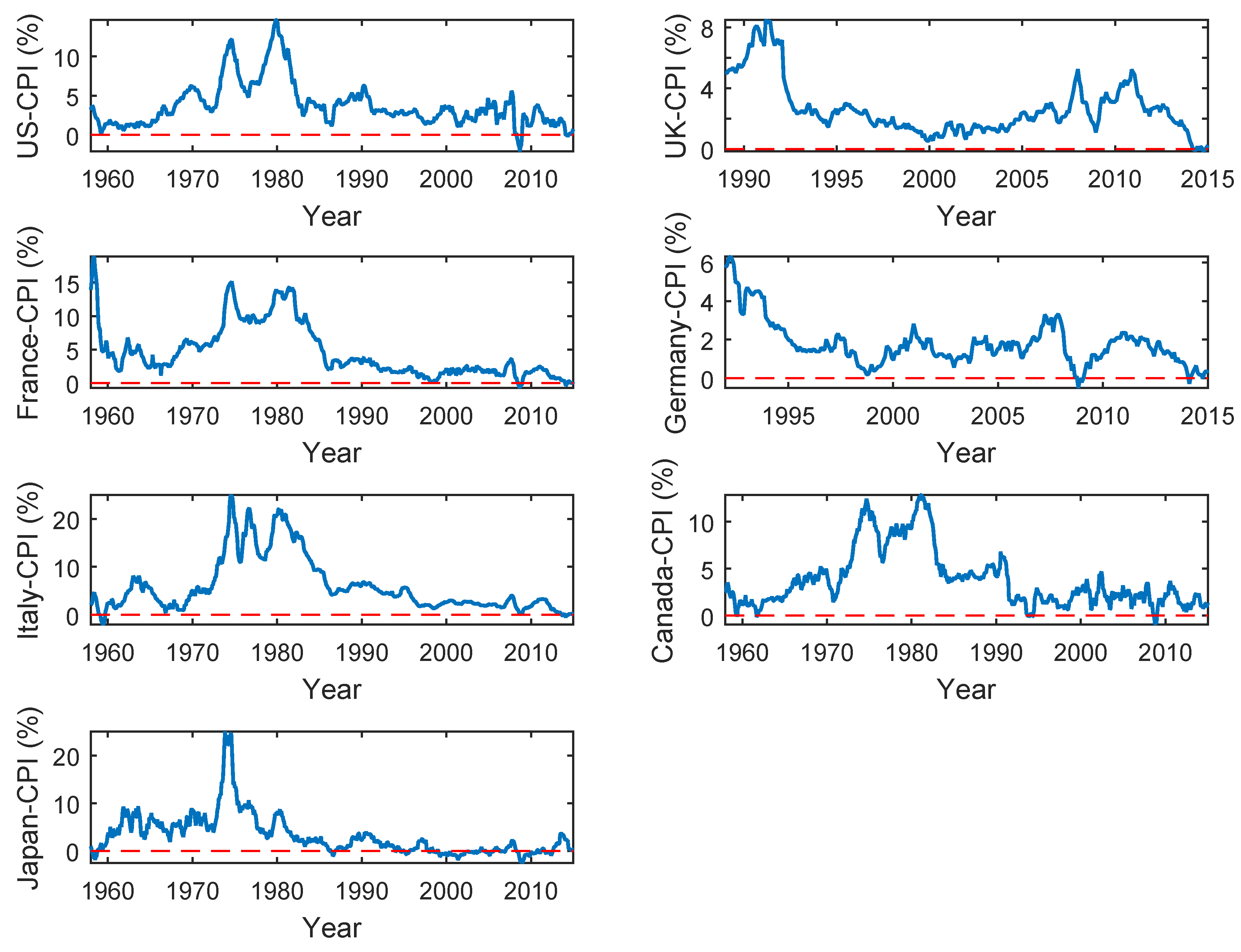
The descriptive statistics of the inflation rates are reported in Table 3. The inflation-rate time series exhibit positive skewness and excess kurtosis (greater than 3) for all G7 countries. This indicates a deviation from the normal distribution that is confirmed by the Jarque-Bera test. To test for stationarity, we apply the Phillips-Perron unit-root test, which does not reject the null hypothesis of a unit root at the 1% level for any of G7 countries (see Table 4). We also apply the KPSS test for the stationarity, the results of which are also reported in Table 4. Here, the null hypothesis of stationarity is rejected for all G7 countries at any conventional significance level. In order to analyze the decay in the tails of the unconditional distributions, we also disclose the country-specific tail indices in Table 3, which range between 2 and 13. For the USA, UK, France, Germany, Italy, and Canada, the tail indices are substantially larger than 2, indicating convergence under time-aggregation towards the normal distribution. For Japan, the tail index is close to 2, indicating that the unconditional distribution exhibits tail behavior like the normal distribution. The results of the ARCH tests in Table 3 suggest the presence of heteroscedasticity in the G7 inflation-rate time series. Figure 1 displays the inflation-rate series.
5.2. Forecasting Methodology
To analyze the predictive ability of our proposed model in forecasting inflation uncertainty, we adopt a rolling forecasting scheme that keeps fixed the estimation sample size over the out-of-sample period and adds new (and removes old) observations on a monthly basis. We define the following in-sample (out-of-sample) periods: (i) January 1958–October 2009 (November 2009–November 2015) for the USA, Canada, and Japan; (ii) January 1989–November 2009 (December 2009–December 2015) for the UK; (iii) January 1958–November 2009 (December 2009–December 2015) for France and Italy; (iv) January 1992–November 2009 (December 2009–December 2015) for Germany. For each country and model specification, we consider inflation uncertainty forecasts for the horizons months. We consider the end of the global financial crisis 2007–2009 as the splitting point in our forecasting analysis.
In a first step, we first evaluate the forecasting performance of our specifications on the basis of two loss functions, (i) the mean squared error (MSE) and (ii) the mean absolute error (MAE), given by
with denoting the volatility forecast obtained from the binomial MSM or GARCH-type models, and the monthly actual inflation uncertainty proxy obtained from the monthly squared residuals from suitably selected STARFIMA model specifications. (Here, T is the number of out-of-sample observations.)
Next, we use of the predictive ability tests of Hansen (2005) and Diebold and Mariano (1995) to test the relative forecasting performance of our proposed specification against competitor models. The Equal Predictive Ability (EPA) test of Diebold and Mariano (1995) enables us to directly compare the forecasting accuracy of two competing models (say, and ) under a predefined loss function. The null hypothesis of no difference in the forecasting accuracy between the competing models is stated as
where , with and denoting the forecast errors obtained from the models and , respectively. The loss function is either the squared error loss or the absolute error loss . The Diebold-Mariano test statistic is given by
where , and is the heteroscedasticity and autocorrelation consistent (HAC) variance estimator. ( is the estimate of the autocovariance function at lag j, N is the nearest integer larger than .) Under the null hypothesis, the test statistic in Equation (16) is asymptotically standard normally distributed.
Based on the framework of the Reality Check (RC) proposed by White (2000), the Superior Predictive Ability (SPA) test of Hansen (2005) enables us to compare a benchmark forecast model, , with K alternative competing models, , under predefined loss functions. The null hypothesis, stating that the benchmark model is not outperformed by any of the K competing models, is formalized as
where for and denotes either the squared-error or the absolute-error loss function, as defined above. To formally state the test statistic, we consider (i) the sample mean of the ith loss differential, , and (ii) the estimated variance for . We refer the reader to Hansen (2005) for the technical details on how to estimate this latter variance by bootstrapping. To test the null hypothesis in Equation (17), we use the test statistic
the p-values of which can be obtained via a stationary bootstrap procedure.
5.3. Forecasting Results
The G7 country-specific root mean squared error (RMSE) and mean absolute error (MAE) values for alternative STARFIMA-MSM and STARFIMA-GARCH-type specifications at the forecasting horizons months are reported in Table 5, Table 6, Table 7 and Table 8. Instead of considering the general STARFIMA() class in modeling our mean process, we restrict attention to two special cases, namely, the STARFI model (by setting ) and the ARFIMA model (by setting for in the lag polynomial on the left side of Equation (1)).
Based on the RMSEs and MAEs in Table 5 and Table 6, the ARFIMA-MSM specification appears to fit best the US and UK inflation rates. For France, Germany, Italy, Canada, and Japan, the ARFIMA-GARCH model yields relatively similar RMSEs and MAEs, that are superior to those of the ARFIMA-MSM model. In order to test whether the observed RMSE- and MAE-differences between the ARFIMA-MSM and -GARCH-type models are statistically significant, we apply the SPA test of Hansen (2005). The p-values obtained from 5000 bootstrap samples using both, the squared and absolute error loss functions, are reported in Table 9 and Table 10. While the null hypothesis (that the ARFIMA-MSM model is not outperformed by any of the ARFIMA-GARCH specifications) cannot be rejected for the US, UK, and France at the 10% level, we find rejection of the null hypothesis for Germany, Italy, Canada, and Japan. We also apply the EPA test in order to compare the ARFIMA-MSM specification with each of the ARFIMA-GARCH-type models (see Table 11 and Table 12). The null hypothesis (no difference in forecast accuracy) can only be rejected for the US, UK, and France (in most cases) at the 10% level. For Germany, Italy, Canada, and Japan, the ARFIMA-MSM and -GARCH models appear to exhibit similar forecasting performance.
When modeling the inflation-rate mean process by the STARFI specification, we obtain substantial gains in forecast accuracy. The RMSEs and MAEs in Table 7 and Table 8 as well as the SPA and EPA tests in Table 13, Table 14, Table 15 and Table 16 indicate that the STARFI-MSM specification systematically outperforms the respective STARFI-GARCH specifications for all G7 countries, except for Japan. Our results suggest that the STARFI-MSM model fits the G7 inflation rates considerably well, thus producing accurate inflation uncertainty forecasts. For Japan, all models perform well, but it appears impossible to find a specific model systematically dominating the others.
6. Conclusions
This paper proposes the ARFIMA- and STAR-MSM models for forecasting inflation uncertainty in the G7 countries. The specifications are found to model the dynamics of inflation uncertainty appropriately, since they are able to capture (i) dual long memory, (ii) clustering effects, (iii) non-linearities, and (iv) asymmetries observed in inflation rates. Our out-of-sample forecasting analysis confirms these capacities and the robustness of our models, which yield accurate forecasts of inflation uncertainty. In particular, the performance of the STARFI-MSM is interesting and should have major implications for monetary policy, which merit careful investigation in future research.
Author Contributions
All authors contributed equally to the paper.
Conflicts of Interest
The authors declare no conflict of interest.
References
- Baillie, Richard T., Ching-Fan Chung, and Margie A. Tieslau. 1996. Analyzing inflation by the fractionally integrated ARFIMA-GARCH model. Journal of Applied Econometrics 11: 23–40. [Google Scholar] [CrossRef]
- Baker, R. Scott, Nicholas Bloom, and Steven J. Davis. 2015. Measuring economic policy uncertainty. Quarterly Journal of Economics 136: 1593–636. [Google Scholar]
- Beran, Jan. 1994. Statistics for Long-memory Processes. New York: Chapman and Hall. [Google Scholar]
- Bernanke, Ben S. 1983. Irreversibility, uncertainty, and cyclical investment. Quarterly Journal of Economics 98: 85–106. [Google Scholar] [CrossRef]
- Bloom, Nicholas. 2009. The impact of uncertainty shocks. Econometrica 77: 623–85. [Google Scholar]
- Bloom, Nicholas. 2014. Fluctuations in uncertainty. Journal of Economic Perspectives 28: 153–76. [Google Scholar] [CrossRef]
- Bollerslev, Tim. 1986. Generalized autoregressive conditional heteroskedasticity. Journal of Econometrics 31: 307–27. [Google Scholar] [CrossRef]
- Calvet, Laurant E., and Adlai J. Fisher. 2001. Forecasting multifractal volatility. Journal of Econometrics 105: 27–58. [Google Scholar] [CrossRef]
- Calvet, Laurant E., and Adlai J. Fisher. 2004. Regime-switching and the estimation of multifractal processes. Journal of Financial Econometrics 2: 44–83. [Google Scholar] [CrossRef]
- Caporale, Guglielmo, Luca Onarante, and Paolo Paesani. 2012. Inflation uncertainty in Euro Aera. Empirical Economics 43: 597–615. [Google Scholar] [CrossRef]
- Clements, Michael P. 2014. Forecast uncertainty—Ex ante and Ex post: US inflation and output growth. Journal of Business and Economic Statistics 32: 206–16. [Google Scholar] [CrossRef]
- Diebold, Francis X., and Roberto S. Mariano. 1995. Comparing predictive accuracy. Journal of Business and Economic Statistics 13: 253–63. [Google Scholar]
- Ding, Zhuanxin, Clive Granger, and Robert Engle. 1993. A long memory property of stock market returns and a new model. Journal of Empirical Finance 1: 83–106. [Google Scholar] [CrossRef]
- Engle, Robert F. 1982. Autoregressive conditional heteroscedasticity with estimates of the variance of United Kingdom inflation. Econometrica 50: 987–1007. [Google Scholar] [CrossRef]
- Fountas, Stilianos, Alexandra Ioannidis, and Menelaos Karanasos. 2004. Inflation, inflation uncertainty and a common European Monetary Policy. Manchester School 2: 221–42. [Google Scholar] [CrossRef]
- Glosten, Lawrence R., Ravi Jagannathan, and David E. Runkle. 1993. On the relation between the expected value and volatility of the nominal excess return on stocks. Journal of Finance 46: 1779–801. [Google Scholar] [CrossRef]
- Goodhart, Charles A. 1999. Central bankers and uncertainty. Bank of England Quarterly Bulletin 39: 102–21. [Google Scholar]
- Greenspan, Alan. 2003. Testimony before the Committee on Banking, Housing, and Urban Affairs. U.S. Senate, 16 July 2003. Technical Report, Federal Reserve Board’s Semiannual Monetary Policy Report to the Congress. Washington: Federal Reserve Board. [Google Scholar]
- Gurkaynak, Refet S., and Jonathan H. Wright. 2012. Macroeconomics and the term structure. Journal of Economic Literature 50: 331–67. [Google Scholar] [CrossRef]
- Hansen, Peter R. 2005. A test for superior predictive ability. Journal of Business and Economic Statistics 23: 365–80. [Google Scholar] [CrossRef]
- He, Changli, and Timo Terasvirta. 1999. Properties of moments of a family of GARCH processes. Journal of Econometrics 92: 173–92. [Google Scholar] [CrossRef]
- Henzel, Steffen R., and Malte Rengel. 2017. Dimensions of macroeconomic uncertainty: A common factor analysis. Economic Inquiry 55: 843–77. [Google Scholar] [CrossRef]
- Hillebrand, Eric, and Marcelo C. Medeiros. 2016. Nonlinearity, breaks and long-range dependence in time-series models. Journal of Business and Economic Statistics 34: 23–41. [Google Scholar] [CrossRef]
- Hosking, Jonathan R. 1981. Fractional differencing. Biometrika 68: 165–76. [Google Scholar] [CrossRef]
- Jurado, Kyle, Sydney C. Ludvigson, and Serena Ng. 2015. Measuring uncertainty. American Economic Review 105: 1177–216. [Google Scholar] [CrossRef]
- Karanasos, Menelaos, and Stefanie Schurer. 2008. Is the relationship between inflation and its uncertainty linear? German Economic Review 9: 265–86. [Google Scholar] [CrossRef]
- Li, Wai Keung, and A. I. McLeod. 1986. Fractional time series modeling. Biometrika 73: 217–21. [Google Scholar] [CrossRef]
- Ling, Shiqing. 1999. On the probabilistic properties of a double threshold ARMA conditional heteroskedasticity model. Journal of Applied Probability 36: 1–18. [Google Scholar] [CrossRef]
- Ling, Shiqing, and Michael McAleer. 2002a. Necessary and sufficient moment conditions for the GARCH(r,s) and asymmetric power GARCH(r,s) models. Econometric Theory 18: 722–29. [Google Scholar] [CrossRef]
- Ling, Shiqing, and Michael McAleer. 2002b. Stationary and the existence of moments of a GARCH processes. Journal of Econometrics 106: 109–17. [Google Scholar] [CrossRef]
- Liu, Ruipeng, Tiziana di Matteo, and Thomas Lux. 2007. True and apparent scaling: The proximity of the Markov-switching multifractal model to long-range dependence. Physica A 383: 35–42. [Google Scholar] [CrossRef]
- Lundbergh, Stefan, and Timo Terasvirta. 1999. Modelling Economic High Frequency Time Series with STAR-STGARCH Models. SSE/EFI Working Paper Series in Economics and Finance, No. 291; Stockholm, Sweden: Stockholm School of Economics. [Google Scholar]
- Lux, Thomas. 2008. The Markov-switching multifractal model of asset returns: GMM estimation and linear forecasting of volatility. Journal of Business and Economic Statistics 26: 194–210. [Google Scholar] [CrossRef]
- Lux, Thomas, and Mawuli Segnon. 2018. Multifractal models in finance: Their origin, properties and applications. In OUP Handbook on Computational Economics and Finance. Edited by Shu-Heng Chen, Mak Kaboudan and Ye-Rong Du. Oxford: Oxford University Press. [Google Scholar]
- Lux, Thomas, Mawuli Segnon, and Rangan Gupta. 2016. Forecasting crude oil price volatility and value-at-risk: Evidence from historical and recent data. Energy Economics 56: 117–33. [Google Scholar] [CrossRef]
- Makarova, Svetlana. 2018. European central bank footprints on inflation forecast uncertainty. Economic Inquiry 56: 637–52. [Google Scholar]
- Nelson, Daniel B. 1991. Conditional heteroskedasticity in asset returns: A new approach. Econometrica 59: 347–70. [Google Scholar] [CrossRef]
- Pötscher, Benedikt, and Ingmar R. Prucha. 1997. Dynamic Nonlinear Econometric Models—Asymptotic Theory. New York: Springer. [Google Scholar]
- Segnon, Mawuli, Thomas Lux, and Rangan Gupta. 2017. Modeling and forecasting the volatility of carbon dioxide emission allowance prices: A review and comparison of modern volatility models. Renewable and Sustainable Energy Reviews 69: 692–704. [Google Scholar] [CrossRef]
- Sentana, Enrique. 1995. Quadratic ARCH models. Review of Economic Studies 62: 639–61. [Google Scholar] [CrossRef]
- Shiryaev, Albert. 1995. Probability (Graduate Texts in Mathematics), 2nd ed.Springer: New York. [Google Scholar]
- Stock, James H., and Mark W. Watson. 2012. Disentangling the Channels of the 2007-09 Recession. NBER Working Paper No. 18094. 1050 Massachusetts Ave., Cambridge, MA, USA: NBER. [Google Scholar]
- Van Dijk, Dick, Timo Terasvirta, and Phillip H. Franses. 2002. Smooth transition autoregressive models—A survey of recent developments. Econometric Reviews 21: 1–47. [Google Scholar] [CrossRef]
- Wang, Yudon, Congfeng Wu, and Li Yang. 2016. Forecasting crude oil market volatility: A Markov switching multifractal volatility approach. International Journal of Forecasting 32: 1–9. [Google Scholar] [CrossRef]
- White, Halbert. 2000. A reality check for data snooping. Econometrica 68: 1097–126. [Google Scholar] [CrossRef]
- Wooldridge, Jeffrey. 1994. Chapter Estimation and Inference for Dependent Processes. In Aspects of Modelling Nonlinear Time Series. Amsterdam: Elsevier Science, pp. 2639–738. [Google Scholar]
- Wright, Jonathan H. 2011. Term premia and inflation uncertainty: Empirical evidence from an international panel dataset. American Economic Review 101: 1514–34. [Google Scholar] [CrossRef]
- Žikeš, Filip, Jozef Baruník, and Nikhil Shenai. 2017. Modeling and forecasting persistent financial durations. Econometric Reviews 36: 1081–110. [Google Scholar] [CrossRef]
| 1 | See Lux and Segnon (2018) for details on the genesis and alternative applications of multifractal processes in finance. |
| 2 | Technical details on the determination of the optimal number of multipliers are available upon request. |
Figure 1.
Consumer-price-index (CPI)-based inflation rates for the G7 countries.


Table 1.
Monte-Carlo maximum-likelihood-estimation results for small sample sizes.
| Binomial parameter | |||||||||
| Bias | −0.036 | −0.028 | −0.010 | −0.025 | −0.023 | −0.036 | −0.022 | −0.027 | −0.018 |
| MSE | 0.005 | 0.003 | 0.001 | 0.004 | 0.002 | 0.002 | 0.003 | 0.002 | 0.001 |
| Scaling factor | |||||||||
| Bias | −0.108 | −0.072 | −0.061 | −0.214 | −0.150 | −0.105 | −0.315 | −0.232 | −0.187 |
| MSE | 0.013 | 0.006 | 0.004 | 0.048 | 0.024 | 0.012 | 0.101 | 0.055 | 0.036 |
Note: The table reports average biases and mean-squared errors (MSEs) of parameter estimates from 500 MSM(k) simulation paths for .
Table 2.
Simulated moments and Hurst exponents via the binomial MSM(k) model.
| G7 Countries | |||||||
|---|---|---|---|---|---|---|---|
| US | UK | France | Germany | Italy | Canada | Japan | |
| Mean | 1.659 × 10 | 9.152 × 10 | −5.509 × 10 | 4.574 × 10 | 0.001 | −1.472× 10 | −6.959 × 10 |
| Standard deviation | 0.283 | 0.260 | 0.317 | 0.224 | 0.281 | 0.365 | 0.737 |
| Skewness | −6.932 × 10 | 0.032 | −0.003 | 0.021 | 0.006 | 0.006 | −0.029 |
| Kurtosis | 4.369 | 7.130 | 5.627 | 5.775 | 8.202 | 4.686 | 8.380 |
| Hurst Exponent for the G7 Countries | |||||||
| 0.499 | 0.491 | 0.508 | 0.504 | 0.515 | 0.499 | 0.508 | |
| 0.673 | 0.814 | 0.780 | 0.772 | 0.867 | 0.694 | 0.901 | |
| 0.630 | 0.773 | 0.766 | 0.721 | 0.813 | 0.673 | 0.848 | |
Note: For each country, we estimate the parameters in the binomial MSM specification and use the estimates to simulate data with country-specific sample sizes corresponding to those of the estimated residuals from the STARFIMA model. The moments and Hurst exponents are averaged over the number of replications.
Table 3.
Descriptive statistics of the G7 inflation-rate time series.
| US | UK | France | Germany | Italy | Canada | Japan | |
|---|---|---|---|---|---|---|---|
| No. of Obs | 696 | 324 | 696 | 288 | 696 | 695 | 695 |
| Mean | 3.778 | 2.643 | 4.582 | 1.771 | 6.004 | 3.815 | 3.157 |
| Standard deviation | 2.864 | 1.802 | 3.980 | 1.171 | 5.739 | 3.082 | 4.264 |
| Skewness | 1.536 | 1.395 | 1.238 | 1.482 | 1.424 | 1.248 | 2.206 |
| Kurtosis | 5.428 | 4.624 | 3.728 | 5.993 | 4.105 | 3.687 | 10.080 |
| Tail index | 7.688 | 11.719 | 12.251 | 6.720 | 10.922 | 13.050 | 2.09 |
| 4.825 × 10 | 2.056 × 10 | 4.769 × 10 | 1.359 × 10 | 5.123 E× 10 | 5.030 × 10 | 4.712 × 10 | |
| ARCH(1) | 685.983 | 309.386 | 684.018 | 271.658 | 684.284 | 684.306 | 660.613 |
| Jarque-Bera | 444.528 | 140.674 | 193.272 | 213.002 | 207.722 | 194.039 | 2.095 × 10 |
Note: denotes the Ljung-Box test for serial correlation out to lag 8. ARCH(1) denotes the Engle test for ARCH effects at lag 1.
Table 4.
Unit root tests for inflation time series.
| Country | PP | PP * | ST | ST * | |
|---|---|---|---|---|---|
| US | −2.044 | −1.876 | 3.634 | 6.001 | |
| UK | −1.851 | −1.669 | 2.101 | 3.963 | |
| France | −2.225 | −2.243 | 2.753 | 13.571 | |
| Germany | −3.357 | −3.363 | 1.148 | 3.495 | |
| Italy | −1.728 | −1.324 | 4.549 | 8.382 | |
| Canada | −2.052 | −1.798 | 4.356 | 8.033 | |
| Japan | −3.119 | −2.345 | 1.704 | 13.913 | |
Note: PP and PP* represent the Phillips-Perron adjusted t-statistics of the lagged dependent variable in a regression with (i) intercept and time trend and (ii) intercept only. The critical values at the 1% level are and . ST and ST denote the KPSS test statistics using residuals from regressions with (i) intercept and time trend and (ii) intercept only. The critical values at the 1% level are and .
Table 5.
Root mean squared errors (RMSEs), mean process: AutoRegressive Fractionally Integrated Moving Average (ARFIMA).
Table 5.
Root mean squared errors (RMSEs), mean process: AutoRegressive Fractionally Integrated Moving Average (ARFIMA).
| Forecasting Horizons | 1M | 2M | 3M | 4M | 5M | 6M | |||||
|---|---|---|---|---|---|---|---|---|---|---|---|
| Countries | GARCH | ||||||||||
| US | 0.179 | 0.184 | 0.187 | 0.183 | 0.178 | 0.173 | |||||
| UK | 0.110 | 0.115 | 0.120 | 0.123 | 0.124 | 0.126 | |||||
| France | 0.065 | 0.065 | 0.066 | 0.067 | 0.068 | 0.069 | |||||
| Germany | 0.078 | 0.077 | 0.076 | 0.069 | 0.068 | 0.066 | |||||
| Italy | 0.076 | 0.078 | 0.078 | 0.078 | 0.078 | 0.078 | |||||
| Canada | 0.213 | 0.210 | 0.210 | 0.211 | 0.209 | 0.209 | |||||
| Japan | 0.512 | 0.510 | 0.509 | 0.508 | 0.505 | 0.506 | |||||
| GJR | |||||||||||
| US | 0.196 | 0.201 | 0.206 | 0.204 | 0.198 | 0.192 | |||||
| UK | 0.117 | 0.119 | 0.121 | 0.125 | 0.128 | 0.130 | |||||
| France | 0.063 | 0.064 | 0.065 | 0.067 | 0.067 | 0.069 | |||||
| Germany | 0.082 | 0.081 | 0.079 | 0.073 | 0.072 | 0.071 | |||||
| Italy | 0.076 | 0.077 | 0.077 | 0.078 | 0.078 | 0.078 | |||||
| Canada | 0.213 | 0.210 | 0.210 | 0.211 | 0.210 | 0.209 | |||||
| Japan | 0.513 | 0.511 | 0.509 | 0.507 | 0.504 | 0.504 | |||||
| EGARCH | |||||||||||
| US | 0.169 | 0.171 | 0.171 | 0.169 | 0.162 | 0.156 | |||||
| UK | 0.117 | 0.115 | 0.116 | 0.116 | 0.116 | 0.117 | |||||
| France | 0.078 | 0.083 | 0.079 | 0.082 | 0.080 | 0.081 | |||||
| Germany | 0.085 | 0.084 | 0.082 | 0.077 | 0.075 | 0.073 | |||||
| Italy | 0.078 | 0.078 | 0.079 | 0.080 | 0.080 | 0.080 | |||||
| Canada | 0.215 | 0.210 | 0.210 | 0.210 | 0.211 | 0.211 | |||||
| Japan | 0.505 | 0.503 | 0.502 | 0.500 | 0.498 | 0.497 | |||||
| QGARCH | |||||||||||
| US | 0.180 | 0.183 | 0.185 | 0.183 | 0.177 | 0.171 | |||||
| UK | 0.103 | 0.104 | 0.106 | 0.107 | 0.108 | 0.110 | |||||
| France | 0.061 | 0.063 | 0.064 | 0.065 | 0.067 | 0.066 | |||||
| Germany | 0.083 | 0.082 | 0.080 | 0.072 | 0.071 | 0.069 | |||||
| Italy | 0.077 | 0.078 | 0.078 | 0.079 | 0.079 | 0.078 | |||||
| Canada | 0.213 | 0.210 | 0.210 | 0.211 | 0.209 | 0.208 | |||||
| Japan | 0.509 | 0.508 | 0.507 | 0.505 | 0.503 | 0.503 | |||||
| APGARCH | |||||||||||
| US | 0.203 | 0.209 | 0.216 | 0.212 | 0.206 | 0.201 | |||||
| UK | 0.120 | 0.123 | 0.123 | 0.128 | 0.128 | 0.125 | |||||
| France | 0.057 | 0.057 | 0.058 | 0.058 | 0.058 | 0.059 | |||||
| Germany | 0.086 | 0.086 | 0.086 | 0.078 | 0.076 | 0.075 | |||||
| Italy | 0.075 | 0.077 | 0.078 | 0.079 | 0.078 | 0.078 | |||||
| Canada | 0.214 | 0.212 | 0.213 | 0.214 | 0.212 | 0.211 | |||||
| Japan | 0.509 | 0.506 | 0.505 | 0.504 | 0.410 | 0.500 | |||||
| MSM | |||||||||||
| US | 0.153 | 0.157 | 0.156 | 0.154 | 0.151 | 0.150 | |||||
| UK | 0.104 | 0.104 | 0.103 | 0.105 | 0.106 | 0.106 | |||||
| France | 0.060 | 0.061 | 0.061 | 0.062 | 0.062 | 0.062 | |||||
| Germany | 0.082 | 0.081 | 0.080 | 0.075 | 0.074 | 0.073 | |||||
| Italy | 0.082 | 0.086 | 0.089 | 0.091 | 0.092 | 0.093 | |||||
| Canada | 0.219 | 0.215 | 0.215 | 0.216 | 0.214 | 0.214 | |||||
| Japan | 0.518 | 0.514 | 0.513 | 0.511 | 0.508 | 0.511 | |||||
Note: RMSEs are computed for the following out-of-sample periods: November 2009–November 2015 for Canada and Japan; December 2009–December 2015 for the US, UK, France, Germany, and Italy. The lag orders in the ARFIMA specification (not displayed here) were obtained from the Bayesian Information Criterion (BIC).
Table 6.
Mean absolute errors (MAEs), mean process: ARFIMA.
| Forecasting Horizons | 1M | 2M | 3M | 4M | 5M | 6M | |||||
|---|---|---|---|---|---|---|---|---|---|---|---|
| Countries | GARCH | ||||||||||
| US | 0.140 | 0.142 | 0.144 | 0.142 | 0.139 | 0.137 | |||||
| UK | 0.083 | 0.088 | 0.091 | 0.094 | 0.093 | 0.096 | |||||
| France | 0.059 | 0.060 | 0.061 | 0.062 | 0.063 | 0.064 | |||||
| Germany | 0.063 | 0.064 | 0.064 | 0.060 | 0.060 | 0.060 | |||||
| Italy | 0.049 | 0.049 | 0.050 | 0.050 | 0.049 | 0.050 | |||||
| Canada | 0.151 | 0.148 | 0.150 | 0.151 | 0.150 | 0.149 | |||||
| Japan | 0.199 | 0.199 | 0.200 | 0.199 | 0.198 | 0.199 | |||||
| GJR | |||||||||||
| US | 0.150 | 0.151 | 0.152 | 0.152 | 0.148 | 0.145 | |||||
| UK | 0.091 | 0.093 | 0.092 | 0.093 | 0.096 | 0.098 | |||||
| France | 0.056 | 0.058 | 0.059 | 0.061 | 0.061 | 0.063 | |||||
| Germany | 0.066 | 0.066 | 0.066 | 0.063 | 0.062 | 0.061 | |||||
| Italy | 0.048 | 0.047 | 0.049 | 0.049 | 0.048 | 0.048 | |||||
| Canada | 0.151 | 0.150 | 0.150 | 0.152 | 0.151 | 0.149 | |||||
| Japan | 0.214 | 0.215 | 0.214 | 0.214 | 0.213 | 0.215 | |||||
| EGARCH | |||||||||||
| US | 0.133 | 0.133 | 0.132 | 0.132 | 0.128 | 0.125 | |||||
| UK | 0.092 | 0.091 | 0.089 | 0.088 | 0.088 | 0.089 | |||||
| France | 0.072 | 0.078 | 0.073 | 0.077 | 0.074 | 0.076 | |||||
| Germany | 0.070 | 0.070 | 0.069 | 0.066 | 0.065 | 0.064 | |||||
| Italy | 0.050 | 0.050 | 0.051 | 0.051 | 0.051 | 0.050 | |||||
| Canada | 0.144 | 0.137 | 0.139 | 0.140 | 0.141 | 0.142 | |||||
| Japan | 0.191 | 0.192 | 0.190 | 0.189 | 0.190 | 0.192 | |||||
| QGARCH | |||||||||||
| US | 0.140 | 0.140 | 0.140 | 0.140 | 0.136 | 0.133 | |||||
| UK | 0.077 | 0.078 | 0.079 | 0.079 | 0.080 | 0.080 | |||||
| France | 0.056 | 0.058 | 0.060 | 0.060 | 0.062 | 0.061 | |||||
| Germany | 0.067 | 0.067 | 0.066 | 0.063 | 0.061 | 0.060 | |||||
| Italy | 0.049 | 0.049 | 0.050 | 0.051 | 0.050 | 0.050 | |||||
| Canada | 0.151 | 0.149 | 0.149 | 0.151 | 0.150 | 0.148 | |||||
| Japan | 0.204 | 0.205 | 0.207 | 0.207 | 0.207 | 0.210 | |||||
| APGARCH | |||||||||||
| US | 0.154 | 0.155 | 0.158 | 0.156 | 0.152 | 0.150 | |||||
| UK | 0.089 | 0.090 | 0.087 | 0.090 | 0.091 | 0.090 | |||||
| France | 0.052 | 0.052 | 0.053 | 0.054 | 0.054 | 0.055 | |||||
| Germany | 0.071 | 0.072 | 0.072 | 0.068 | 0.067 | 0.067 | |||||
| Italy | 0.048 | 0.048 | 0.050 | 0.050 | 0.048 | 0.049 | |||||
| Canada | 0.155 | 0.154 | 0.155 | 0.157 | 0.154 | 0.154 | |||||
| Japan | 0.186 | 0.188 | 0.186 | 0.187 | 0.188 | 0.190 | |||||
| MSM | |||||||||||
| US | 0.123 | 0.126 | 0.127 | 0.126 | 0.123 | 0.122 | |||||
| UK | 0.080 | 0.082 | 0.081 | 0.082 | 0.084 | 0.086 | |||||
| France | 0.051 | 0.052 | 0.053 | 0.054 | 0.054 | 0.055 | |||||
| Germany | 0.067 | 0.068 | 0.068 | 0.066 | 0.065 | 0.064 | |||||
| Italy | 0.063 | 0.066 | 0.071 | 0.073 | 0.074 | 0.077 | |||||
| Canada | 0.162 | 0.159 | 0.161 | 0.163 | 0.161 | 0.161 | |||||
| Japan | 0.216 | 0.219 | 0.227 | 0.231 | 0.234 | 0.240 | |||||
Note: MAEs are computed for the following out-of-sample periods: November 2009–November 2015 for Canada and Japan; December 2009–December 2015 for the US, UK, France, Germany, and Italy. The lag orders in the ARFIMA specification (not displayed here) were obtained from the Bayesian Information Criterion (BIC).
Table 7.
Root mean squared errors (RMSEs), mean process: Smooth Transition AutoRegressive Fractionally Integrated (STARFI).
Table 7.
Root mean squared errors (RMSEs), mean process: Smooth Transition AutoRegressive Fractionally Integrated (STARFI).
| Forecasting Horizons | 1M | 2M | 3M | 4M | 5M | 6M | |||||
|---|---|---|---|---|---|---|---|---|---|---|---|
| Countries | GARCH | ||||||||||
| US | 0.176 | 0.181 | 0.184 | 0.179 | 0.173 | 0.169 | |||||
| UK | 0.108 | 0.113 | 0.112 | 0.114 | 0.118 | 0.120 | |||||
| France | 0.067 | 0.067 | 0.067 | 0.068 | 0.068 | 0.069 | |||||
| Germany | 0.080 | 0.080 | 0.079 | 0.072 | 0.071 | 0.070 | |||||
| Italy | 0.075 | 0.076 | 0.076 | 0.076 | 0.076 | 0.076 | |||||
| Canada | 0.206 | 0.203 | 0.203 | 0.204 | 0.203 | 0.203 | |||||
| Japan | 0.516 | 0.514 | 0.513 | 0.511 | 0.509 | 0.509 | |||||
| GJR | |||||||||||
| US | 0.192 | 0.197 | 0.203 | 0.202 | 0.195 | 0.190 | |||||
| UK | 0.121 | 0.115 | 0.117 | 0.122 | 0.125 | 0.129 | |||||
| France | 0.066 | 0.066 | 0.067 | 0.068 | 0.068 | 0.069 | |||||
| Germany | 0.082 | 0.083 | 0.081 | 0.076 | 0.075 | 0.074 | |||||
| Italy | 0.074 | 0.075 | 0.075 | 0.075 | 0.075 | 0.075 | |||||
| Canada | 0.205 | 0.203 | 0.202 | 0.205 | 0.203 | 0.204 | |||||
| Japan | 0.517 | 0.515 | 0.513 | 0.511 | 0.507 | 0.508 | |||||
| EGARCH | |||||||||||
| US | 0.169 | 0.171 | 0.172 | 0.170 | 0.163 | 0.157 | |||||
| UK | 0.117 | 0.117 | 0.118 | 0.119 | 0.119 | 0.122 | |||||
| France | 0.078 | 0.084 | 0.079 | 0.081 | 0.080 | 0.081 | |||||
| Germany | 0.086 | 0.085 | 0.083 | 0.077 | 0.075 | 0.078 | |||||
| Italy | 0.077 | 0.077 | 0.077 | 0.078 | 0.078 | 0.078 | |||||
| Canada | 0.209 | 0.203 | 0.203 | 0.204 | 0.204 | 0.205 | |||||
| Japan | 0.508 | 0.507 | 0.506 | 0.503 | 0.501 | 0.503 | |||||
| QGARCH | |||||||||||
| US | 0.176 | 0.179 | 0.181 | 0.180 | 0.173 | 0.167 | |||||
| UK | 0.105 | 0.105 | 0.107 | 0.109 | 0.110 | 0.112 | |||||
| France | 0.061 | 0.060 | 0.059 | 0.060 | 0.060 | 0.060 | |||||
| Germany | 0.085 | 0.085 | 0.082 | 0.076 | 0.075 | 0.074 | |||||
| Italy | 0.076 | 0.076 | 0.077 | 0.077 | 0.077 | 0.077 | |||||
| Canada | 0.206 | 0.203 | 0.202 | 0.204 | 0.202 | 0.202 | |||||
| Japan | 0.513 | 0.512 | 0.510 | 0.508 | 0.506 | 0.508 | |||||
| APGARCH | |||||||||||
| US | 0.193 | 0.202 | 0.210 | 0.204 | 0.198 | 0.194 | |||||
| UK | 0.111 | 0.118 | 0.121 | 0.126 | 0.130 | 0.128 | |||||
| France | 0.060 | 0.060 | 0.061 | 0.061 | 0.062 | 0.062 | |||||
| Germany | 0.086 | 0.086 | 0.092 | 0.084 | 0.082 | 0.082 | |||||
| Italy | 0.073 | 0.076 | 0.076 | 0.076 | 0.075 | 0.074 | |||||
| Canada | 0.205 | 0.204 | 0.206 | 0.206 | 0.204 | 0.204 | |||||
| Japan | 0.512 | 0.509 | 0.507 | 0.505 | 0.503 | 0.504 | |||||
| MSM | |||||||||||
| US | 0.155 | 0.158 | 0.158 | 0.155 | 0.152 | 0.151 | |||||
| UK | 0.103 | 0.103 | 0.102 | 0.104 | 0.104 | 0.105 | |||||
| France | 0.061 | 0.061 | 0.061 | 0.062 | 0.062 | 0.062 | |||||
| Germany | 0.083 | 0.084 | 0.083 | 0.078 | 0.077 | 0.076 | |||||
| Italy | 0.082 | 0.086 | 0.088 | 0.089 | 0.089 | 0.091 | |||||
| Canada | 0.213 | 0.208 | 0.208 | 0.210 | 0.208 | 0.208 | |||||
| Japan | 0.522 | 0.518 | 0.517 | 0.515 | 0.511 | 0.515 | |||||
Note: RMSEs are computed for the following out-of-sample periods: November 2009–November 2015 for Canada and Japan; December 2009–December 2015 for the US, UK, France, Germany, and Italy. The lag orders in the STARFI specification (not displayed here) were obtained from the Bayesian Information Criterion (BIC).
Table 8.
Mean absolute errors (MAEs), mean process: STARFI.
| Forecasting Horizons | 1M | 2M | 3M | 4M | 5M | 6M | |||||
|---|---|---|---|---|---|---|---|---|---|---|---|
| Countries | GARCH | ||||||||||
| US | 0.136 | 0.138 | 0.138 | 0.136 | 0.133 | 0.131 | |||||
| UK | 0.081 | 0.087 | 0.086 | 0.088 | 0.091 | 0.093 | |||||
| France | 0.062 | 0.062 | 0.062 | 0.063 | 0.063 | 0.064 | |||||
| Germany | 0.064 | 0.064 | 0.064 | 0.061 | 0.061 | 0.060 | |||||
| Italy | 0.049 | 0.049 | 0.050 | 0.049 | 0.048 | 0.050 | |||||
| Canada | 0.152 | 0.149 | 0.150 | 0.151 | 0.150 | 0.149 | |||||
| Japan | 0.198 | 0.197 | 0.200 | 0.199 | 0.198 | 0.200 | |||||
| GJR | |||||||||||
| US | 0.142 | 0.144 | 0.146 | 0.145 | 0.142 | 0.141 | |||||
| UK | 0.095 | 0.091 | 0.090 | 0.094 | 0.097 | 0.097 | |||||
| France | 0.060 | 0.060 | 0.061 | 0.062 | 0.063 | 0.064 | |||||
| Germany | 0.065 | 0.066 | 0.066 | 0.063 | 0.062 | 0.061 | |||||
| Italy | 0.046 | 0.047 | 0.047 | 0.047 | 0.047 | 0.047 | |||||
| Canada | 0.150 | 0.149 | 0.149 | 0.152 | 0.152 | 0.151 | |||||
| Japan | 0.216 | 0.216 | 0.217 | 0.217 | 0.216 | 0.218 | |||||
| EGARCH | |||||||||||
| US | 0.128 | 0.129 | 0.129 | 0.128 | 0.123 | 0.121 | |||||
| UK | 0.093 | 0.093 | 0.092 | 0.091 | 0.092 | 0.093 | |||||
| France | 0.072 | 0.078 | 0.074 | 0.075 | 0.075 | 0.075 | |||||
| Germany | 0.071 | 0.070 | 0.068 | 0.067 | 0.066 | 0.067 | |||||
| Italy | 0.050 | 0.050 | 0.051 | 0.052 | 0.051 | 0.052 | |||||
| Canada | 0.147 | 0.140 | 0.142 | 0.143 | 0.144 | 0.145 | |||||
| Japan | 0.192 | 0.193 | 0.194 | 0.194 | 0.195 | 0.198 | |||||
| QGARCH | |||||||||||
| US | 0.132 | 0.132 | 0.134 | 0.134 | 0.130 | 0.127 | |||||
| UK | 0.081 | 0.080 | 0.083 | 0.083 | 0.084 | 0.084 | |||||
| France | 0.055 | 0.055 | 0.055 | 0.056 | 0.056 | 0.055 | |||||
| Germany | 0.067 | 0.068 | 0.066 | 0.064 | 0.063 | 0.061 | |||||
| Italy | 0.049 | 0.049 | 0.050 | 0.050 | 0.050 | 0.051 | |||||
| Canada | 0.151 | 0.149 | 0.149 | 0.152 | 0.150 | 0.149 | |||||
| Japan | 0.204 | 0.206 | 0.208 | 0.209 | 0.209 | 0.213 | |||||
| APGARCH | |||||||||||
| US | 0.144 | 0.149 | 0.151 | 0.146 | 0.143 | 0.143 | |||||
| UK | 0.085 | 0.091 | 0.088 | 0.091 | 0.094 | 0.093 | |||||
| France | 0.055 | 0.055 | 0.056 | 0.057 | 0.057 | 0.057 | |||||
| Germany | 0.072 | 0.073 | 0.075 | 0.070 | 0.070 | 0.069 | |||||
| Italy | 0.046 | 0.048 | 0.049 | 0.047 | 0.046 | 0.047 | |||||
| Canada | 0.153 | 0.151 | 0.154 | 0.156 | 0.152 | 0.152 | |||||
| Japan | 0.185 | 0.187 | 0.186 | 0.188 | 0.189 | 0.192 | |||||
| MSM | |||||||||||
| US | 0.123 | 0.126 | 0.126 | 0.124 | 0.122 | 0.122 | |||||
| UK | 0.081 | 0.082 | 0.081 | 0.082 | 0.084 | 0.085 | |||||
| France | 0.052 | 0.052 | 0.053 | 0.054 | 0.054 | 0.055 | |||||
| Germany | 0.067 | 0.068 | 0.068 | 0.066 | 0.065 | 0.064 | |||||
| Italy | 0.062 | 0.066 | 0.070 | 0.072 | 0.073 | 0.076 | |||||
| Canada | 0.163 | 0.159 | 0.161 | 0.162 | 0.159 | 0.160 | |||||
| Japan | 0.214 | 0.219 | 0.226 | 0.230 | 0.233 | 0.239 | |||||
Note: MAEs are computed for the following out-of-sample periods: November 2009–November 2015 for Canada and Japan; December 2009–December 2015 for the US, UK, France, Germany, and Italy. The lag orders in the STARFI specification (not displayed here) were obtained from the Bayesian Information Criterion (BIC).
Table 9.
Superior Predictive Ability (SPA) test, squared error loss, mean process: ARFIMA.
| Forecasting Horizons | 1M | 2M | 3M | 4M | 5M | 6M | |||||
|---|---|---|---|---|---|---|---|---|---|---|---|
| Benchmark Models | US | ||||||||||
| GARCH | 0.088 | 0.066 | 0.047 | 0.070 | 0.049 | 0.045 | |||||
| GJR | 0.034 | 0.032 | 0.026 | 0.024 | 0.021 | 0.039 | |||||
| EGARCH | 0.055 | 0.088 | 0.081 | 0.072 | 0.143 | 0.284 | |||||
| QGARCH | 0.041 | 0.047 | 0.041 | 0.031 | 0.031 | 0.032 | |||||
| APGARCH | 0.038 | 0.038 | 0.031 | 0.031 | 0.033 | 0.043 | |||||
| MSM | 1.000 | 1.000 | 1.000 | 1.000 | 0.857 | 0.716 | |||||
| UK | |||||||||||
| GARCH | 0.110 | 0.255 | 0.094 | 0.031 | 0.164 | 0.109 | |||||
| GJR | 0.017 | 0.028 | 0.036 | 0.034 | 0.033 | 0.031 | |||||
| EGARCH | 0.046 | 0.122 | 0.086 | 0.134 | 0.161 | 0.100 | |||||
| QGARCH | 0.621 | 0.748 | 0.259 | 0.328 | 0.287 | 0.208 | |||||
| APGARCH | 0.070 | 0.051 | 0.058 | 0.061 | 0.057 | 0.109 | |||||
| MSM | 0.379 | 0.735 | 0.741 | 0.672 | 0.713 | 0.792 | |||||
| France | |||||||||||
| GARCH | 0.006 | 0.002 | 0.001 | 0.001 | 0.000 | 0.000 | |||||
| GJR | 0.053 | 0.026 | 0.020 | 0.010 | 0.002 | 0.001 | |||||
| EGARCH | 0.000 | 0.000 | 0.000 | 0.000 | 0.000 | 0.000 | |||||
| QGARCH | 0.080 | 0.006 | 0.004 | 0.001 | 0.000 | 0.000 | |||||
| APGARCH | 0.780 | 0.856 | 0.821 | 0.859 | 0.839 | 1.000 | |||||
| MSM | 0.274 | 0.172 | 0.224 | 0.179 | 0.161 | 0.145 | |||||
| Germany | |||||||||||
| GARCH | 1.000 | 1.000 | 1.000 | 1.000 | 1.000 | 1.000 | |||||
| GJR | 0.020 | 0.049 | 0.076 | 0.016 | 0.034 | 0.037 | |||||
| EGARCH | 0.009 | 0.018 | 0.022 | 0.005 | 0.008 | 0.007 | |||||
| QGARCH | 0.012 | 0.021 | 0.064 | 0.037 | 0.075 | 0.091 | |||||
| APGARCH | 0.013 | 0.006 | 0.002 | 0.005 | 0.005 | 0.004 | |||||
| MSM | 0.055 | 0.049 | 0.101 | 0.010 | 0.011 | 0.016 | |||||
| Italy | |||||||||||
| GARCH | 0.240 | 0.367 | 0.232 | 0.474 | 0.553 | 0.476 | |||||
| GJR | 0.245 | 0.717 | 0.898 | 0.926 | 0.599 | 0.559 | |||||
| EGARCH | 0.092 | 0.202 | 0.144 | 0.151 | 0.061 | 0.109 | |||||
| QGARCH | 0.099 | 0.180 | 0.141 | 0.160 | 0.053 | 0.134 | |||||
| APGARCH | 0.781 | 0.770 | 0.312 | 0.387 | 0.765 | 0.785 | |||||
| MSM | 0.018 | 0.012 | 0.003 | 0.001 | 0.000 | 0.000 | |||||
| Canada | |||||||||||
| GARCH | 0.953 | 0.869 | 0.582 | 0.840 | 0.803 | 0.791 | |||||
| GJR | 0.727 | 0.521 | 0.630 | 0.450 | 0.431 | 0.416 | |||||
| EGARCH | 0.383 | 0.558 | 0.549 | 0.598 | 0.437 | 0.347 | |||||
| QGARCH | 0.802 | 0.838 | 0.951 | 0.870 | 0.993 | 0.998 | |||||
| APGARCH | 0.468 | 0.116 | 0.048 | 0.139 | 0.154 | 0.125 | |||||
| MSM | 0.004 | 0.059 | 0.025 | 0.041 | 0.033 | 0.005 | |||||
| Japan | |||||||||||
| GARCH | 0.210 | 0.267 | 0.217 | 0.238 | 0.114 | 0.172 | |||||
| GJR | 0.130 | 0.188 | 0.267 | 0.268 | 0.379 | 0.148 | |||||
| EGARCH | 0.749 | 0.733 | 0.993 | 0.993 | 0.853 | 0.764 | |||||
| QGARCH | 0.047 | 0.037 | 0.031 | 0.017 | 0.018 | 0.015 | |||||
| APGARCH | 0.373 | 0.492 | 0.451 | 0.400 | 0.541 | 0.350 | |||||
| MSM | 0.063 | 0.060 | 0.052 | 0.014 | 0.029 | 0.013 | |||||
Note: The displayed numbers are the p-values of the SPA test of Hansen (2005) using the squared error loss. We test the null hypothesis that the benchmark model is not outperformed by any of the other candidate models. The p-values are obtained for the following out-of-sample periods: November 2009–November 2015 for Canada and Japan; December 2009–December 2015 for the US, UK, France, Germany, and Italy. The inflation-rate mean process is ARFIMA.
Table 10.
Superior Predictive Ability (SPA) test, absolute error loss, mean process: ARFIMA.
| Forecasting Horizons | 1M | 2M | 3M | 4M | 5M | 6M | |||||
|---|---|---|---|---|---|---|---|---|---|---|---|
| Benchmark Models | US | ||||||||||
| GARCH | 0.075 | 0.032 | 0.014 | 0.026 | 0.025 | 0.018 | |||||
| GJR | 0.024 | 0.014 | 0.0150 | 0.017 | 0.017 | 0.028 | |||||
| EGARCH | 0.089 | 0.156 | 0.180 | 0.168 | 0.236 | 0.346 | |||||
| QGARCH | 0.053 | 0.076 | 0.036 | 0.052 | 0.078 | 0.051 | |||||
| APGARCH | 0.023 | 0.020 | 0.009 | 0.016 | 0.023 | 0.030 | |||||
| MSM | 1.000 | 0.844 | 0.820 | 0.832 | 0.764 | 0.678 | |||||
| UK | |||||||||||
| GARCH | 0.136 | 0.130 | 0.057 | 0.016 | 0.098 | 0.058 | |||||
| GJR | 0.007 | 0.004 | 0.014 | 0.012 | 0.003 | 0.002 | |||||
| EGARCH | 0.0122 | 0.020 | 0.051 | 0.073 | 0.050 | 0.036 | |||||
| QGARCH | 0.814 | 1.000 | 0.742 | 0.802 | 1.000 | 1.000 | |||||
| APGARCH | 0.058 | 0.043 | 0.159 | 0.058 | 0.049 | 0.091 | |||||
| MSM | 0.258 | 0.145 | 0.375 | 0.265 | 0.175 | 0.155 | |||||
| France | |||||||||||
| GARCH | 0.001 | 0.000 | 0.000 | 0.000 | 0.000 | 0.000 | |||||
| GJR | 0.008 | 0.003 | 0.001 | 0.000 | 0.000 | 0.000 | |||||
| EGARCH | 0.000 | 0.000 | 0.000 | 0.000 | 0.000 | 0.000 | |||||
| QGARCH | 0.098 | 0.004 | 0.001 | 0.002 | 0.000 | 0.001 | |||||
| APGARCH | 0.359 | 0.537 | 0.470 | 0.544 | 0.542 | 0.578 | |||||
| MSM | 0.641 | 0.463 | 0.530 | 0.456 | 0.458 | 0.422 | |||||
| Germany | |||||||||||
| GARCH | 1.000 | 1.000 | 0.847 | 1.000 | 0.756 | 0.691 | |||||
| GJR | 0.161 | 0.154 | 0.204 | 0.123 | 0.188 | 0.229 | |||||
| EGARCH | 0.006 | 0.007 | 0.014 | 0.004 | 0.004 | 0.003 | |||||
| QGARCH | 0.086 | 0.105 | 0.250 | 0.220 | 0.393 | 0.484 | |||||
| APGARCH | 0.033 | 0.018 | 0.006 | 0.012 | 0.008 | 0.001 | |||||
| MSM | 0.009 | 0.010 | 0.020 | 0.010 | 0.016 | 0.031 | |||||
| Italy | |||||||||||
| GARCH | 0.272 | 0.204 | 0.249 | 0.402 | 0.271 | 0.200 | |||||
| GJR | 0.611 | 1.000 | 1.000 | 0.913 | 0.822 | 0.715 | |||||
| EGARCH | 0.062 | 0.065 | 0.063 | 0.082 | 0.052 | 0.133 | |||||
| QGARCH | 0.045 | 0.024 | 0.030 | 0.043 | 0.012 | 0.060 | |||||
| APGARCH | 0.630 | 0.281 | 0.063 | 0.374 | 0.559 | 0.462 | |||||
| MSM | 0.000 | 0.000 | 0.000 | 0.000 | 0.000 | 0.000 | |||||
| Canada | |||||||||||
| GARCH | 0.365 | 0.084 | 0.066 | 0.094 | 0.139 | 0.261 | |||||
| GJR | 0.268 | 0.078 | 0.087 | 0.096 | 0.112 | 0.200 | |||||
| EGARCH | 0.880 | 1.000 | 1.000 | 1.000 | 1.000 | 1.000 | |||||
| QGARCH | 0.388 | 0.091 | 0.092 | 0.102 | 0.155 | 0.337 | |||||
| APGARCH | 0.050 | 0.012 | 0.010 | 0.006 | 0.036 | 0.009 | |||||
| MSM | 0.000 | 0.000 | 0.000 | 0.000 | 0.000 | 0.000 | |||||
| Japan | |||||||||||
| GARCH | 0.121 | 0.162 | 0.092 | 0.140 | 0.179 | 0.175 | |||||
| GJR | 0.007 | 0.007 | 0.003 | 0.003 | 0.004 | 0.003 | |||||
| EGARCH | 0.433 | 0.469 | 0.271 | 0.373 | 0.377 | 0.542 | |||||
| QGARCH | 0.045 | 0.039 | 0.013 | 0.007 | 0.010 | 0.005 | |||||
| APGARCH | 0.731 | 0.704 | 0.729 | 0.627 | 0.623 | 0.651 | |||||
| MSM | 0.006 | 0.001 | 0.000 | 0.000 | 0.000 | 0.000 | |||||
Note: The displayed numbers are the p-values of the SPA test of Hansen (2005) using the absolute error loss. We test the null hypothesis that the benchmark model is not outperformed by any of the other candidate models. The p-values are obtained for the following out-of-sample periods: November 2009–November 2015 for Canada and Japan; December 2009–December 2015 for the US, UK, France, Germany, and Italy. The inflation-rate mean process is ARFIMA.
Table 11.
Equal Predictive Ability (EPA) test, squared error loss, mean process: ARFIMA.
| Forecasting Horizons | |||||||
|---|---|---|---|---|---|---|---|
| Model 1 | Model 2 | 1M | 2M | 3M | 4M | 5M | 6M |
| US | |||||||
| GARCH | MSM | 0.026 | 0.087 | 0.087 | 0.068 | 0.136 | 0.192 |
| GJR | 0.015 | 0.067 | 0.074 | 0.055 | 0.106 | 0.155 | |
| EGARCH | 0.045 | 0.140 | 0.142 | 0.066 | 0.169 | 0.308 | |
| QGARCH | 0.022 | 0.084 | 0.086 | 0.050 | 0.118 | 0.190 | |
| APGARCH | 0.012 | 0.064 | 0.066 | 0.061 | 0.113 | 0.154 | |
| UK | |||||||
| GARCH | MSM | 0.057 | 0.163 | 0.034 | 0.021 | 0.120 | 0.067 |
| GJR | 0.018 | 0.059 | 0.092 | 0.135 | 0.148 | 0.162 | |
| EGARCH | 0.054 | 0.089 | 0.079 | 0.158 | 0.194 | 0.167 | |
| QGARCH | 0.633 | 0.549 | 0.317 | 0.397 | 0.382 | 0.334 | |
| APGARCH | 0.037 | 0.073 | 0.107 | 0.144 | 0.168 | 0.204 | |
| France | |||||||
| GARCH | MSM | 0.011 | 0.020 | 0.010 | 0.023 | 0.002 | 0.002 |
| GJR | 0.009 | 0.020 | 0.012 | 0.004 | 0.000 | 0.000 | |
| EGARCH | 0.000 | 0.000 | 0.000 | 0.000 | 0.000 | 0.000 | |
| QGARCH | 0.395 | 0.349 | 0.278 | 0.322 | 0.192 | 0.251 | |
| APGARCH | 0.777 | 0.800 | 0.728 | 0.745 | 0.718 | 0.706 | |
| Germany | |||||||
| GARCH | MSM | 0.965 | 0.969 | 0.930 | 0.958 | 0.940 | 0.919 |
| GJR | 0.464 | 0.633 | 0.670 | 0.806 | 0.825 | 0.791 | |
| EGARCH | 0.040 | 0.136 | 0.225 | 0.360 | 0.403 | 0.402 | |
| QGARCH | 0.284 | 0.382 | 0.558 | 0.760 | 0.776 | 0.751 | |
| APGARCH | 0.127 | 0.126 | 0.083 | 0.343 | 0.380 | 0.363 | |
| Italy | |||||||
| GARCH | MSM | 0.947 | 0.968 | 0.979 | 0.985 | 0.987 | 0.9871 |
| GJR | 0.890 | 0.966 | 0.980 | 0.982 | 0.981 | 0.981 | |
| EGARCH | 0.783 | 0.929 | 0.956 | 0.963 | 0.959 | 0.966 | |
| QGARCH | 0.846 | 0.950 | 0.971 | 0.975 | 0.970 | 0.976 | |
| APGARCH | 0.969 | 0.967 | 0.968 | 0.971 | 0.981 | 0.984 | |
| Canada | |||||||
| GARCH | MSM | 0.995 | 0.972 | 0.977 | 0.978 | 0.974 | 0.996 |
| GJR | 0.997 | 0.951 | 0.959 | 0.927 | 0.926 | 0.972 | |
| EGARCH | 0.738 | 0.747 | 0.791 | 0.797 | 0.689 | 0.677 | |
| QGARCH | 0.995 | 0.966 | 0.978 | 0.967 | 0.975 | 0.996 | |
| APGARCH | 0.991 | 0.814 | 0.743 | 0.853 | 0.846 | 0.981 | |
| Japan | |||||||
| GARCH | MSM | 0.937 | 0.831 | 0.772 | 0.736 | 0.657 | 0.809 |
| GJR | 0.729 | 0.658 | 0.675 | 0.701 | 0.691 | 0.941 | |
| EGARCH | 0.988 | 0.985 | 0.968 | 0.976 | 0.917 | 0.996 | |
| QGARCH | 0.966 | 0.946 | 0.893 | 0.922 | 0.823 | 0.973 | |
| APGARCH | 0.996 | 0.987 | 0.931 | 0.879 | 0.877 | 0.986 | |
Note: The displayed number are p-values of the EPA test of Diebold and Mariano (1995) using the squared error loss. We test the null hypothesis that the forecasts at horizon h of Model 1 are equal to those of Model 2 against the one-sided alternative that forecasts of Model 1 are inferior to those of Model 2. The p-values are obtained for the following out-of-sample periods: November 2009–November 2015 for Canada and Japan; December 2009–December 2015 for the US, UK, France, Germany, and Italy. The inflation-rate mean process is ARFIMA.
Table 12.
Equal Predictive Ability (EPA) test, absolute error loss, mean process: ARFIMA.
| Forecasting Horizons | |||||||
|---|---|---|---|---|---|---|---|
| Model 1 | Model 2 | 1M | 2M | 3M | 4M | 5M | 6M |
| US | |||||||
| GARCH | MSM | 0.015 | 0.085 | 0.099 | 0.128 | 0.185 | 0.225 |
| GJR | 0.010 | 0.064 | 0.089 | 0.108 | 0.158 | 0.206 | |
| EGARCH | 0.057 | 0.216 | 0.256 | 0.254 | 0.330 | 0.416 | |
| QGARCH | 0.021 | 0.126 | 0.159 | 0.173 | 0.237 | 0.293 | |
| APGARCH | 0.007 | 0.056 | 0.063 | 0.093 | 0.151 | 0.189 | |
| UK | |||||||
| GARCH | MSM | 0.246 | 0.149 | 0.054 | 0.045 | 0.188 | 0.102 |
| GJR | 0.024 | 0.086 | 0.142 | 0.191 | 0.199 | 0.200 | |
| EGARCH | 0.036 | 0.127 | 0.166 | 0.271 | 0.351 | 0.371 | |
| QGARCH | 0.834 | 0.835 | 0.696 | 0.724 | 0.775 | 0.764 | |
| APGARCH | 0.086 | 0.170 | 0.301 | 0.266 | 0.328 | 0.384 | |
| France | |||||||
| GARCH | MSM | 0.000 | 0.000 | 0.000 | 0.001 | 0.000 | 0.000 |
| GJR | 0.000 | 0.000 | 0.000 | 0.000 | 0.000 | 0.000 | |
| EGARCH | 0.000 | 0.000 | 0.000 | 0.000 | 0.000 | 0.000 | |
| QGARCH | 0.046 | 0.049 | 0.059 | 0.122 | 0.060 | 0.099 | |
| APGARCH | 0.324 | 0.515 | 0.464 | 0.515 | 0.514 | 0.532 | |
| Germany | |||||||
| GARCH | MSM | 0.999 | 0.993 | 0.963 | 0.957 | 0.930 | 0.891 |
| GJR | 0.833 | 0.917 | 0.917 | 0.935 | 0.956 | 0.939 | |
| EGARCH | 0.055 | 0.167 | 0.315 | 0.435 | 0.480 | 0.467 | |
| QGARCH | 0.494 | 0.641 | 0.804 | 0.844 | 0.855 | 0.826 | |
| APGARCH | 0.086 | 0.137 | 0.156 | 0.289 | 0.334 | 0.307 | |
| Italy | |||||||
| GARCH | MSM | 1.000 | 1.000 | 1.000 | 1.000 | 1.000 | 1.000 |
| GJR | 1.000 | 1.000 | 1.000 | 1.000 | 1.000 | 1.000 | |
| EGARCH | 1.000 | 1.000 | 1.000 | 1.000 | 1.000 | 1.000 | |
| QGARCH | 1.000 | 1.000 | 1.000 | 1.000 | 1.000 | 1.000 | |
| APGARCH | 1.000 | 1.000 | 1.000 | 1.000 | 1.000 | 1.000 | |
| Canada | |||||||
| GARCH | MSM | 1.000 | 1.000 | 1.000 | 1.000 | 1.000 | 1.000 |
| GJR | 1.000 | 0.999 | 0.999 | 0.997 | 0.991 | 0.997 | |
| EGARCH | 0.995 | 0.997 | 0.999 | 0.999 | 0.997 | 0.991 | |
| QGARCH | 1.000 | 1.000 | 1.000 | 1.000 | 1.000 | 1.000 | |
| APGARCH | 0.996 | 0.958 | 0.976 | 0.986 | 0.998 | 0.999 | |
| Japan | |||||||
| GARCH | MSM | 1.000 | 1.000 | 1.000 | 1.000 | 1.000 | 1.000 |
| GJR | 0.563 | 0.634 | 0.777 | 0.836 | 0.860 | 0.899 | |
| EGARCH | 0.997 | 0.991 | 0.994 | 0.996 | 0.995 | 0.999 | |
| QGARCH | 0.983 | 0.969 | 0.982 | 0.992 | 0.993 | 0.997 | |
| APGARCH | 1.000 | 1.000 | 1.000 | 1.000 | 1.000 | 1.000 | |
Note: The displayed number are p-values of the EPA test of Diebold and Mariano (1995) using the absolute error loss. We test the null hypothesis that the forecasts at horizon h of Model 1 are equal to those of Model 2 against the one-sided alternative that forecasts of Model 1 are inferior to those of Model 2. The p-values are obtained for the following out-of-sample periods: November 2009–November 2015 for Canada and Japan; December 2009–December 2015 for the US, UK, France, Germany, and Italy. The inflation-rate mean process is ARFIMA.
Table 13.
Superior Predictive Ability (SPA) test, squared error loss, mean process: STARFI.
| Forecasting Horizons | 1M | 2M | 3M | 4M | 5M | 6M | |||||
|---|---|---|---|---|---|---|---|---|---|---|---|
| Benchmark Models | US | ||||||||||
| GARCH | 0.108 | 0.068 | 0.051 | 0.099 | 0.058 | 0.038 | |||||
| GJR | 0.041 | 0.036 | 0.027 | 0.029 | 0.024 | 0.041 | |||||
| EGARCH | 0.081 | 0.111 | 0.094 | 0.081 | 0.142 | 0.292 | |||||
| QGARCH | 0.049 | 0.053 | 0.037 | 0.027 | 0.026 | 0.052 | |||||
| APGARCH | 0.058 | 0.047 | 0.035 | 0.052 | 0.045 | 0.055 | |||||
| MSM | 1.000 | 1.000 | 0.906 | 1.000 | 0.858 | 0.737 | |||||
| UK | |||||||||||
| GARCH | 0.197 | 0.099 | 0.088 | 0.044 | 0.080 | 0.063 | |||||
| GJR | 0.004 | 0.045 | 0.077 | 0.048 | 0.040 | 0.034 | |||||
| EGARCH | 0.026 | 0.046 | 0.066 | 0.080 | 0.092 | 0.062 | |||||
| QGARCH | 0.542 | 0.280 | 0.101 | 0.145 | 0.142 | 0.120 | |||||
| APGARCH | 0.217 | 0.080 | 0.050 | 0.068 | 0.055 | 0.101 | |||||
| MSM | 0.715 | 0.720 | 1.000 | 1.000 | 1.000 | 1.000 | |||||
| France | |||||||||||
| GARCH | 0.001 | 0.001 | 0.000 | 0.000 | 0.000 | 0.000 | |||||
| GJR | 0.029 | 0.012 | 0.006 | 0.003 | 0.001 | 0.000 | |||||
| EGARCH | 0.000 | 0.000 | 0.000 | 0.000 | 0.000 | 0.000 | |||||
| QGARCH | 0.623 | 0.817 | 0.719 | 0.776 | 0.758 | 0.833 | |||||
| APGARCH | 0.798 | 0.685 | 0.058 | 0.145 | 0.028 | 0.022 | |||||
| MSM | 0.422 | 0.360 | 0.318 | 0.254 | 0.283 | 0.195 | |||||
| Germany | |||||||||||
| GARCH | 1.000 | 0.901 | 1.000 | 1.000 | 1.000 | 1.000 | |||||
| GJR | 0.094 | 0.050 | 0.090 | 0.034 | 0.049 | 0.034 | |||||
| EGARCH | 0.023 | 0.056 | 0.095 | 0.040 | 0.090 | 0.005 | |||||
| QGARCH | 0.036 | 0.030 | 0.068 | 0.038 | 0.044 | 0.026 | |||||
| APGARCH | 0.150 | 0.171 | 0.007 | 0.007 | 0.001 | 0.004 | |||||
| MSM | 0.092 | 0.036 | 0.030 | 0.008 | 0.007 | 0.010 | |||||
| Italy | |||||||||||
| GARCH | 0.052 | 0.108 | 0.103 | 0.318 | 0.341 | 0.188 | |||||
| GJR | 0.263 | 1.000 | 1.000 | 0.942 | 0.542 | 0.397 | |||||
| EGARCH | 0.004 | 0.021 | 0.013 | 0.005 | 0.006 | 0.022 | |||||
| QGARCH | 0.044 | 0.023 | 0.019 | 0.013 | 0.004 | 0.019 | |||||
| APGARCH | 0.801 | 0.271 | 0.177 | 0.368 | 0.849 | 0.775 | |||||
| MSM | 0.007 | 0.006 | 0.003 | 0.000 | 0.001 | 0.000 | |||||
| Canada | |||||||||||
| GARCH | 0.638 | 0.801 | 0.350 | 0.914 | 0.875 | 0.722 | |||||
| GJR | 0.743 | 0.796 | 0.653 | 0.657 | 0.517 | 0.352 | |||||
| EGARCH | 0.356 | 0.612 | 0.510 | 0.622 | 0.447 | 0.381 | |||||
| QGARCH | 0.824 | 0.978 | 0.918 | 0.939 | 0.988 | 0.999 | |||||
| APGARCH | 0.795 | 0.453 | 0.108 | 0.529 | 0.419 | 0.512 | |||||
| MSM | 0.006 | 0.077 | 0.033 | 0.076 | 0.028 | 0.002 | |||||
| Japan | |||||||||||
| GARCH | 0.217 | 0.266 | 0.219 | 0.224 | 0.1456 | 0.198 | |||||
| GJR | 0.109 | 0.158 | 0.200 | 0.199 | 0.327 | 0.225 | |||||
| EGARCH | 0.712 | 0.680 | 0.985 | 0.987 | 0.907 | 0.995 | |||||
| QGARCH | 0.054 | 0.031 | 0.024 | 0.010 | 0.008 | 0.018 | |||||
| APGARCH | 0.430 | 0.561 | 0.543 | 0.514 | 0.459 | 0.388 | |||||
| MSM | 0.052 | 0.035 | 0.059 | 0.011 | 0.010 | 0.030 | |||||
Note: The displayed numbers are the p-values of the SPA test of Hansen (2005) using the squared error loss. We test the null hypothesis that the benchmark model is not outperformed by any of the other candidate models. The p-values are obtained for the following out-of-sample periods: November 2009–November 2015 for Canada and Japan; December 2009–December 2015 for the US, UK, France, Germany, and Italy. The inflation-rate mean process is STARFI.
Table 14.
Superior Predictive Ability (SPA) test, absolute error loss, mean process: STARFI.
| Forecasting Horizons | 1M | 2M | 3M | 4M | 5M | 6M | |||||
|---|---|---|---|---|---|---|---|---|---|---|---|
| Models | US | ||||||||||
| GARCH | 0.000 | 0.000 | 0.000 | 0.000 | 0.000 | 0.000 | |||||
| GJR | 0.000 | 0.000 | 0.000 | 0.000 | 0.000 | 0.000 | |||||
| EGARCH | 0.000 | 0.000 | 0.000 | 0.000 | 0.000 | 0.000 | |||||
| QGARCH | 0.000 | 0.000 | 0.000 | 0.000 | 0.000 | 0.000 | |||||
| APGARCH | 0.000 | 0.000 | 0.000 | 0.000 | 0.000 | 0.000 | |||||
| MSM | 1.000 | 1.000 | 1.000 | 1.000 | 1.000 | 1.000 | |||||
| UK | |||||||||||
| GARCH | 0.000 | 0.000 | 0.000 | 0.000 | 0.000 | 0.000 | |||||
| GJR | 0.000 | 0.000 | 0.000 | 0.000 | 0.000 | 0.000 | |||||
| EGARCH | 0.000 | 0.000 | 0.000 | 0.000 | 0.000 | 0.000 | |||||
| QGARCH | 0.000 | 0.000 | 0.000 | 0.000 | 0.000 | 0.000 | |||||
| APGARCH | 0.000 | 0.000 | 0.000 | 0.000 | 0.000 | 0.000 | |||||
| MSM | 1.000 | 1.000 | 1.000 | 1.000 | 1.000 | 1.000 | |||||
| France | |||||||||||
| GARCH | 0.000 | 0.000 | 0.000 | 0.000 | 0.000 | 0.000 | |||||
| GJR | 0.000 | 0.000 | 0.000 | 0.000 | 0.000 | 0.000 | |||||
| EGARCH | 0.000 | 0.000 | 0.000 | 0.000 | 0.000 | 0.000 | |||||
| QGARCH | 0.000 | 0.000 | 0.000 | 0.000 | 0.000 | 0.000 | |||||
| APGARCH | 0.000 | 0.000 | 0.000 | 0.000 | 0.000 | 0.000 | |||||
| MSM | 1.000 | 1.000 | 1.000 | 1.000 | 1.000 | 1.000 | |||||
| Germany | |||||||||||
| GARCH | 0.000 | 0.000 | 0.000 | 0.000 | 0.000 | 0.000 | |||||
| GJR | 0.000 | 0.000 | 0.000 | 0.000 | 0.000 | 0.000 | |||||
| EGARCH | 0.000 | 0.000 | 0.000 | 0.000 | 0.000 | 0.000 | |||||
| QGARCH | 0.000 | 0.000 | 0.000 | 0.000 | 0.000 | 0.000 | |||||
| APGARCH | 0.000 | 0.000 | 0.000 | 0.000 | 0.000 | 0.000 | |||||
| MSM | 1.000 | 1.000 | 1.000 | 1.000 | 1.000 | 1.000 | |||||
| Italy | |||||||||||
| GARCH | 0.000 | 0.000 | 0.000 | 0.000 | 0.000 | 0.000 | |||||
| GJR | 0.000 | 0.000 | 0.000 | 0.000 | 0.000 | 0.000 | |||||
| EGARCH | 0.000 | 0.000 | 0.000 | 0.000 | 0.000 | 0.000 | |||||
| QGARCH | 0.000 | 0.000 | 0.000 | 0.000 | 0.000 | 0.000 | |||||
| APGARCH | 0.000 | 0.000 | 0.000 | 0.000 | 0.000 | 0.000 | |||||
| MSM | 1.000 | 1.000 | 1.000 | 1.000 | 1.000 | 1.000 | |||||
| Canada | |||||||||||
| GARCH | 0.000 | 0.000 | 0.000 | 0.000 | 0.000 | 0.000 | |||||
| GJR | 0.000 | 0.000 | 0.000 | 0.000 | 0.000 | 0.000 | |||||
| EGARCH | 0.000 | 0.000 | 0.000 | 0.000 | 0.000 | 0.000 | |||||
| QGARCH | 0.000 | 0.000 | 0.000 | 0.000 | 0.000 | 0.000 | |||||
| APGARCH | 0.000 | 0.000 | 0.000 | 0.000 | 0.000 | 0.000 | |||||
| MSM | 1.000 | 1.000 | 1.000 | 1.000 | 1.000 | 1.000 | |||||
| Japan | |||||||||||
| GARCH | 0.115 | 0.174 | 0.101 | 0.148 | 0.179 | 0.217 | |||||
| GJR | 0.006 | 0.007 | 0.004 | 0.004 | 0.006 | 0.008 | |||||
| EGARCH | 0.395 | 0.437 | 0.390 | 0.443 | 0.450 | 0.441 | |||||
| QGARCH | 0.041 | 0.046 | 0.022 | 0.016 | 0.020 | 0.014 | |||||
| APGARCH | 0.931 | 0.935 | 0.936 | 0.935 | 0.934 | 0.931 | |||||
| MSM | 0.229 | 0.243 | 0.239 | 0.244 | 0.252 | 0.257 | |||||
Note: The displayed numbers are the p-values of the SPA test of Hansen (2005) using the absolute error loss. We test the null hypothesis that the benchmark model is not outperformed by any of the other candidate models. The p-values are obtained for the following out-of-sample periods: November 2009–November 2015 for Canada and Japan; December 2009–December 2015 for the US, UK, France, Germany, and Italy. The inflation-rate mean process is STARFI.
Table 15.
Equal Predictive Ability (EPA) test, squared error loss, mean process: STARFI.
| Forecasting Horizons | |||||||
|---|---|---|---|---|---|---|---|
| Model 1 | Model 2 | 1M | 2M | 3M | 4M | 5M | 6M |
| US | |||||||
| GARCH | MSM | 0.030 | 0.094 | 0.096 | 0.081 | 0.149 | 0.210 |
| GJR | 0.023 | 0.081 | 0.086 | 0.070 | 0.119 | 0.163 | |
| EGARCH | 0.068 | 0.167 | 0.158 | 0.096 | 0.186 | 0.319 | |
| QGARCH | 0.040 | 0.112 | 0.105 | 0.064 | 0.134 | 0.215 | |
| APGARCH | 0.024 | 0.081 | 0.076 | 0.078 | 0.134 | 0.173 | |
| UK | |||||||
| GARCH | MSM | 0.093 | 0.056 | 0.045 | 0.069 | 0.073 | 0.086 |
| GJR | 0.001 | 0.072 | 0.118 | 0.136 | 0.152 | 0.161 | |
| EGARCH | 0.015 | 0.057 | 0.088 | 0.147 | 0.183 | 0.170 | |
| QGARCH | 0.277 | 0.306 | 0.153 | 0.233 | 0.264 | 0.262 | |
| APGARCH | 0.099 | 0.077 | 0.081 | 0.130 | 0.155 | 0.187 | |
| France | |||||||
| GARCH | MSM | 0.003 | 0.006 | 0.008 | 0.018 | 0.004 | 0.003 |
| GJR | 0.005 | 0.005 | 0.003 | 0.004 | 0.000 | 0.000 | |
| EGARCH | 0.000 | 0.000 | 0.000 | 0.000 | 0.000 | 0.000 | |
| QGARCH | 0.553 | 0.610 | 0.634 | 0.674 | 0.650 | 0.690 | |
| APGARCH | 0.587 | 0.600 | 0.493 | 0.587 | 0.493 | 0.554 | |
| Germany | |||||||
| GARCH | MSM | 0.970 | 0.981 | 0.963 | 0.968 | 0.953 | 0.934 |
| GJR | 0.651 | 0.700 | 0.771 | 0.866 | 0.864 | 0.823 | |
| EGARCH | 0.212 | 0.371 | 0.500 | 0.573 | 0.674 | 0.389 | |
| QGARCH | 0.245 | 0.357 | 0.577 | 0.727 | 0.740 | 0.706 | |
| APGARCH | 0.265 | 0.301 | 0.038 | 0.098 | 0.115 | 0.044 | |
| Italy | |||||||
| GARCH | MSM | 0.976 | 0.983 | 0.984 | 0.989 | 0.987 | 0.988 |
| GJR | 0.960 | 0.981 | 0.981 | 0.980 | 0.976 | 0.980 | |
| EGARCH | 0.899 | 0.964 | 0.965 | 0.957 | 0.955 | 0.968 | |
| QGARCH | 0.920 | 0.967 | 0.965 | 0.960 | 0.953 | 0.970 | |
| APGARCH | 0.988 | 0.973 | 0.966 | 0.973 | 0.977 | 0.985 | |
| Canada | |||||||
| GARCH | MSM | 0.994 | 0.966 | 0.971 | 0.970 | 0.969 | 0.995 |
| GJR | 0.994 | 0.935 | 0.951 | 0.878 | 0.876 | 0.902 | |
| EGARCH | 0.775 | 0.783 | 0.779 | 0.792 | 0.693 | 0.714 | |
| QGARCH | 0.995 | 0.958 | 0.974 | 0.947 | 0.974 | 0.996 | |
| APGARCH | 0.993 | 0.886 | 0.703 | 0.907 | 0.855 | 0.983 | |
| Japan | |||||||
| GARCH | MSM | 0.931 | 0.833 | 0.766 | 0.741 | 0.677 | 0.813 |
| GJR | 0.696 | 0.637 | 0.649 | 0.684 | 0.716 | 0.935 | |
| EGARCH | 0.980 | 0.986 | 0.972 | 0.989 | 0.959 | 0.988 | |
| QGARCH | 0.954 | 0.949 | 0.905 | 0.945 | 0.881 | 0.944 | |
| APGARCH | 0.997 | 0.994 | 0.964 | 0.947 | 0.897 | 0.969 | |
Note: The displayed number are p-values of the EPA test of Diebold and Mariano (1995) using the squared error loss. We test the null hypothesis that the forecasts at horizon h of Model 1 are equal to those of Model 2 against the one-sided alternative that forecasts of Model 1 are inferior to those of Model 2. The p-values are obtained for the following out-of-sample periods: November 2009–November 2015 for Canada and Japan; December 2009–December 2015 for the US, UK, France, Germany, and Italy. The inflation-rate mean process is STARFI.
Table 16.
Equal Predictive Ability (EPA) test, absolute error loss, mean-process: STARFI.
| Forecasting Horizons | |||||||
|---|---|---|---|---|---|---|---|
| Model 1 | Model 2 | 1M | 2M | 3M | 4M | 5M | 6M |
| US | |||||||
| GARCH | MSM | 0.000 | 0.000 | 0.000 | 0.000 | 0.000 | 0.000 |
| GJR | 0.000 | 0.000 | 0.000 | 0.000 | 0.000 | 0.000 | |
| EGARCH | 0.000 | 0.000 | 0.000 | 0.000 | 0.000 | 0.000 | |
| QGARCH | 0.000 | 0.000 | 0.000 | 0.000 | 0.000 | 0.000 | |
| APGARCH | 0.000 | 0.000 | 0.000 | 0.000 | 0.000 | 0.001 | |
| UK | |||||||
| GARCH | MSM | 0.000 | 0.000 | 0.000 | 0.000 | 0.000 | 0.000 |
| GJR | 0.000 | 0.000 | 0.000 | 0.000 | 0.000 | 0.000 | |
| EGARCH | 0.000 | 0.000 | 0.000 | 0.000 | 0.000 | 0.000 | |
| QGARCH | 0.000 | 0.000 | 0.000 | 0.000 | 0.000 | 0.000 | |
| APGARCH | 0.000 | 0.000 | 0.000 | 0.000 | 0.000 | 0.000 | |
| France | |||||||
| GARCH | MSM | 0.000 | 0.000 | 0.000 | 0.000 | 0.000 | 0.000 |
| GJR | 0.000 | 0.000 | 0.000 | 0.000 | 0.000 | 0.000 | |
| EGARCH | 0.000 | 0.000 | 0.000 | 0.000 | 0.000 | 0.000 | |
| QGARCH | 0.000 | 0.000 | 0.000 | 0.000 | 0.000 | 0.000 | |
| APGARCH | 0.000 | 0.000 | 0.000 | 0.000 | 0.000 | 0.000 | |
| Germany | |||||||
| GARCH | MSM | 0.000 | 0.000 | 0.000 | 0.000 | 0.000 | 0.000 |
| GJR | 0.000 | 0.000 | 0.000 | 0.000 | 0.000 | 0.000 | |
| EGARCH | 0.000 | 0.000 | 0.000 | 0.000 | 0.000 | 0.000 | |
| QGARCH | 0.000 | 0.000 | 0.000 | 0.000 | 0.000 | 0.000 | |
| APGARCH | 0.000 | 0.000 | 0.000 | 0.000 | 0.000 | 0.000 | |
| Italy | |||||||
| GARCH | MSM | 0.000 | 0.000 | 0.000 | 0.000 | 0.000 | 0.000 |
| GJR | 0.000 | 0.000 | 0.000 | 0.000 | 0.000 | 0.000 | |
| EGARCH | 0.000 | 0.000 | 0.000 | 0.000 | 0.000 | 0.000 | |
| QGARCH | 0.000 | 0.000 | 0.000 | 0.000 | 0.000 | 0.000 | |
| APGARCH | 0.000 | 0.000 | 0.000 | 0.000 | 0.000 | 0.000 | |
| Canada | |||||||
| GARCH | MSM | 0.000 | 0.000 | 0.000 | 0.000 | 0.000 | 0.000 |
| GJR | 0.000 | 0.000 | 0.000 | 0.000 | 0.000 | 0.000 | |
| EGARCH | 0.000 | 0.000 | 0.000 | 0.000 | 0.000 | 0.000 | |
| QGARCH | 0.000 | 0.000 | 0.000 | 0.000 | 0.000 | 0.000 | |
| APGARCH | 0.000 | 0.000 | 0.000 | 0.000 | 0.000 | 0.000 | |
| Japan | |||||||
| GARCH | MSM | 0.738 | 0.738 | 0.736 | 0.742 | 0.746 | 0.759 |
| GJR | 0.684 | 0.679 | 0.680 | 0.684 | 0.692 | 0.711 | |
| EGARCH | 0.754 | 0.752 | 0.761 | 0.769 | 0.779 | 0.795 | |
| QGARCH | 0.719 | 0.714 | 0.711 | 0.713 | 0.717 | 0.726 | |
| APGARCH | 0.775 | 0.769 | 0.779 | 0.781 | 0.787 | 0.794 | |
Note: The displayed number are p-values of the EPA test of Diebold and Mariano (1995) using the absolute error loss. We test the null hypothesis that the forecasts at horizon h of Model 1 are equal to those of Model 2 against the one-sided alternative that forecasts of Model 1 are inferior to those of Model 2. The p-values are obtained for the following out-of-sample periods: November 2009–November 2015 for Canada and Japan; December 2009–December 2015 for the US, UK, France, Germany, and Italy. The inflation-rate mean process is STARFI.
© 2018 by the authors. Licensee MDPI, Basel, Switzerland. This article is an open access article distributed under the terms and conditions of the Creative Commons Attribution (CC BY) license (http://creativecommons.org/licenses/by/4.0/).
Share and Cite
MDPI and ACS Style
Segnon, M.; Bekiros, S.; Wilfling, B. Forecasting Inflation Uncertainty in the G7 Countries. Econometrics 2018, 6, 23. https://doi.org/10.3390/econometrics6020023
AMA Style
Segnon M, Bekiros S, Wilfling B. Forecasting Inflation Uncertainty in the G7 Countries. Econometrics. 2018; 6(2):23. https://doi.org/10.3390/econometrics6020023
Chicago/Turabian StyleSegnon, Mawuli, Stelios Bekiros, and Bernd Wilfling. 2018. "Forecasting Inflation Uncertainty in the G7 Countries" Econometrics 6, no. 2: 23. https://doi.org/10.3390/econometrics6020023
Note that from the first issue of 2016, this journal uses article numbers instead of page numbers. See further details here.