Satellite-Detected Carbon Monoxide Pollution during 2000–2012: Examining Global Trends and also Regional Anthropogenic Periods over China, the EU and the USA

Abstract

In this paper, we test if any statistically significant periodicities are detectable in carbon monoxide emissions over China, the European Union, and the United States of America. To do this, we performed a period analysis using 10 years of daily-averaged data, from the Measurements Of Pollution In The Troposphere (MOPITT) instrument. Besides a seasonal period, we found no clearly detectable periods at any timescale with the exception of a strong signal at 2.28 days. This period was observed over all tested regions and persisted when larger (hemisphere-wide) regions were considered. However, rather than resulting from a physical variation in carbon monoxide, it resulted from day-to-day changes in the area covered by MOPITT on-board its polar-orbiting satellite platform. We also examined linear trends over the dataset, and found that MOPITT identifies several centers of increasing carbon monoxide concentration—the largest being over China—although globally MOPITT reports a significant decrease in carbon monoxide has occurred over the past decade.

1. Introduction

Anthropogenic emissions may have important effects on the Earth’s climate connected with the indirect impacts of aerosols on clouds [1,2,3]. Uncertainties regarding the indirect impact of aerosols on the climate system hinder our ability to accurately project future climate scenarios [4]. A useful method of constraining the magnitude of these largely unknown effects is to attempt to identify periodic fluctuations in anthropogenic emissions distinct from natural variability, and then determine if (and by how much) these fluctuations relate to any corresponding changes in meteorology.

In particular, the seven day working week provides an excellent opportunity to test the aerosol indirect effect. Studies of the working week have focused on differences in pollution or meteorological properties either as: a sinusoidal periodicity; a statistical day of the week variation; or a weekend compared to weekday effect. Collectively, these are referred to as evidences of the weekly cycle (WC).

Studies have shown variability in pollution and meteorology corresponding to weekly cycles at local-to-regional scales (e.g., [5,6,7,8,9,10]). Significant weekly cycles have also been reported away from localized centers of urban activity over national scales [11,12], and even at hemispheric [13,14], and global scales [15]. Furthermore, evidence indicates that weekly cycles are not only confined to the troposphere, but also occur in the stratosphere [16]. The wide horizontal and vertical extent of weekly cycle detections suggests that there may be interactions between aerosols and atmospheric dynamics [12]. Studies investigating weekly cycles have recently been reviewed by Sanchez-Lorenzo et al. [17]: althogh evidence is accumulating supporting the existence of weekly cycles, the findings are not yet consistent or conclusive (e.g., [18,19]). Additionally, the studies of weekly cycles are complicated by results which demonstrate that the timing of weekly cycles may vary across regional scales [16], and also that the phase of localized signals may vary over time—this implies that quasi-weekly cycles of natural origin may also be occurring, and interfering with analyses [17].

Weekly cycle effects have also been reported in meteorological parameters such as diurnal temperature, humidity, and rainfall [8,20]—supporting the existence of an indirect link between aerosols and cloud properties (particularly precipitation). Model results support the idea that variations in sulphate aerosols over Europe experienced during a weekly cycle may indeed significantly alter cloud droplet numbers [9]. Local to regional scale trends in boundary layer pollution relating to changes in human activity have also been investigated, and have in some cases suggested long-term correlations exist between cloud properties such as precipitation and aerosols (e.g., [20,21,22,23,24]), although these results have also been conflicting [25,26,27].

In this work, we examine a satellite-detected measurement of tropospheric pollution at a regional-to-hemispheric scale, focusing on the regions of China, Europe, and the United States of America. We aim to provide an assessment independent to those derived from frequently used aerosol and meteorological data—which may be problematic to measure over similar spatio-temporal scales [28,29]. Specifically, we examine carbon monoxide (CO), a common emission product which has been routinely measured by ground-based networks since 1988 [30], and by satellite-based instrumentation for more than a decade [31]. While CO has natural sources, it is also a common byproduct of internal combustion technology and biomass burning, and as such it is found in high concentrations over centers of human activity [32].

2. Data

Our data are from the Measurements of Pollution In The Troposphere (MOPITT) instrument, developed by the Canadian Space Agency (CSA). MOPITT operates on-board the National Aeronautics and Space Administration’s (NASA) polar-orbiting Terra (EOS-AM1) satellite, launched 18 December 1999. It became operational in March 2000, and has since been providing data almost continually on the horizontal and vertical concentrations of tropospheric carbon monoxide (CO) globally [33]. This dataset has been used for a wide range of atmospheric science purposes, and has provided invaluable information over its more-than 10 years of operation [34].

The MOPITT data used in this analysis are a daily-averaged, multi-spectral, version 5 level 3, TIR/NIR product, obtained from the NASA Langley Research Center Atmospheric Science Data Center [35]. MOPITT operates in several spectral channels, utilizing thermal-infrared (TIR) measurements under nighttime conditions (for land and ocean pixels), and near-infrared (NIR) channels during daytime only conditions (for land and ocean pixels) [36]. In the case of measurements over land during daytime both TIR and NIR observations are made (referred to in this work as combined retrievals). The combined use of TIR and NIR observations and updates to the retrieval algorithm for version 5 gives the dataset a significant improvement in retrieval performance compared to older versions of the data [35].

Several short gaps exist in the MOPITT dataset of up to a few weeks in duration; these are mainly due to infrequent (<1 per year) calibration or decontamination events. Additionally, there is a gap in the data from 7 May 2001–24 August 2001 due to a mechanical failure in the MOPITT instrument [37].

MOPITT collects data every 0.4 s, with a pixel size of 484 km${}^2$, and a sensor swath width of 640 km, achieving global coverage over an approximately three-day period. The MOPITT data is particularly sensitive to CO in the middle troposphere (∼500 mb): as potential a limitation to this experiment, we note that MOPITT is only weakly sensitive to CO in the lower troposphere, where the primary sources of CO are situated. MOPITT uses principles of gas correlation radiometry to detect profiles of tropospheric CO and CH${}_4$ under clear-sky (cloud free) conditions: for details regarding this method see [38]. We note that data at latitudes greater than 65${}^{\circ }$ are prone to errors resulting from difficulties in cloud detection over ice covered surfaces.

A validation of the version 5 product is described in [39]. In earlier versions of the MOPITT data, total column CO was found to show a significant positive bias of around 20% compared to in situ measurements, and an increase in this bias over time due to instrumental drift [40,41]. The version 5 data posses an enhanced near-surface CO sensitivity relative to version 4, and a consideration of geophysical noise which resulted from motion of the field of view and surface heterogeneity affecting earlier MOPITT datasets Deeter et al. [35]. Despite this, the version 5 dataset contains effects of instrumental drift, known to be responsible for linear increases in upper and middle troposphere CO concentrations of 2 and 1 ppbv/year in the version 4 dataset Deeter et al. [41]. The updates made to the version 5 dataset mean that the total column CO may exhibit different absolute bias, vertical dependence, and drift than earlier versions of the dataset: comparison to ground-based observations over the USA region indicate retrieval biases in the version 5 data are on the order of a few percent, varying over season and location [36]. Version 5 data exhibit reduced long-term errors compared to earlier datasets, as erroneous long-term changes in pressure and temperature measurements have been explicitly accounted for. We shall briefly consider the long-term statistics of the dataset in Section 3.2.

It is possible that diurnal variations in anthropogenic emissions (particularly those from vehicles) may produce one of the strongest periodicities potentially detectable in pollution data: numerous studies have demonstrated diurnal changes in local pollution occur as a result of changes in traffic density and vehicle type over the course of a 24 h period (e.g., [42,43,44,45,46]). However, our analysis is insensitive to periodicities operating at timescales of <1 day. For our purposes, the detection of a period related to a 7-day week in pollution would be highly useful, whereas, the detection of a diurnal period in pollution would not be (as cloud properties themselves have a diurnal periodicity)—we would need to identify a periodicity clearly distinguishable from natural cloud-rhythms in order to examine the potential impacts of the indirect aerosol effect on clouds [8]. As such, while there is good reason to suspect anthropogenic diurnal periodicities may exist in the MOPITT data (as has been shown in MODIS data [8]), we make no attempt to identify these periods, and use daily-averaged data, making our experiment insensitive to sub-daily periods. Similarly, we apply a 50-day smoothing to the dataset to remove seasonal variations prior to our period analysis—this limits the longest periodicity we may reliably detect to ∼20 days. Therefore, our experiment is restricted to examining MOPITT data for periodicities between 1 and 20 days in length.

3. Analysis

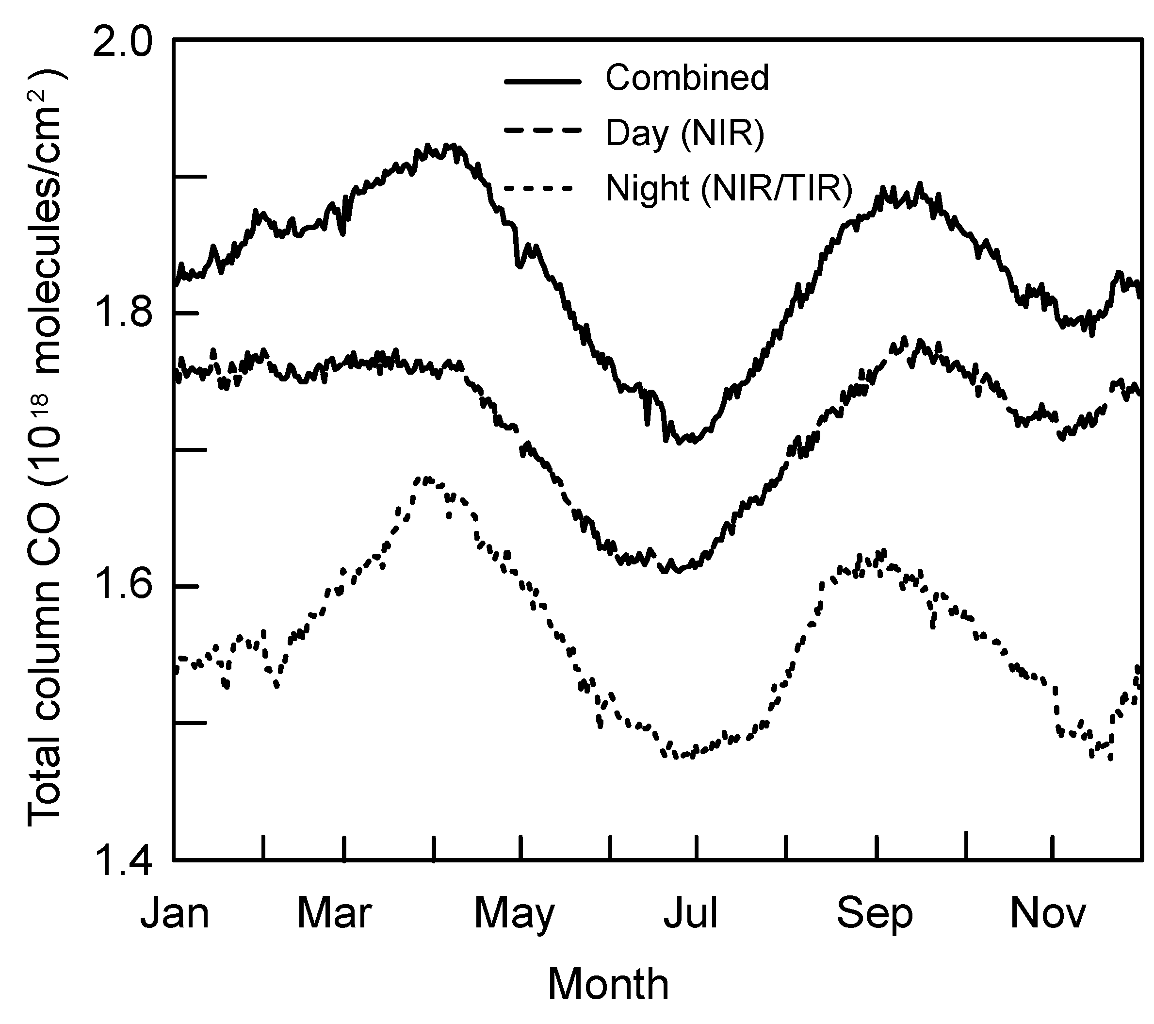
3.1. Globally Averaged CO Values

The daytime (NIR/TIR), nighttime (TIR), and combined daily-averaged global MOPITT data are presented in Figure 1 over the period of 3 March 2000–11 April 2012 for the variable “Retrieved CO Total Column”. The daytime and nighttime data both show a mean of 1.72 × 10${}^{18}$ molecules/cm${}^2$ respectively, and a ±1 standard error of the mean (SEM), of 1.45 and 1.12 × 10${}^{15}$ molecules/cm${}^2$. The daytime/nighttime datasets show a statistically significant correlation coefficient of r = 0.77 ($p<0.01$). We find that although the daytime data demonstrate higher levels of variability, the two datasets show a close agreement, and we proceeded under the assumption that the combined data provide more accurate CO values than the individual (daytime/nighttime) datasets alone.

Regarding the total column CO values (molecules/cm${}^2$) recorded by MOPITT (shown on the y-axis of Figure 1), we note that the absolute values vary between daytime and nighttime retrievals as, firstly, the measurement techniques have different sensitivity, and secondly, the sensor is viewing a different region of the globe under the day-side (daytime) and night-side (nighttime) conditions on the same calendar day. Consequently, the combined retrievals shown in Figure 1c (i.e., retrievals where both NIR/TIR are used in conjunction where available), are not an average of the data in Figure 1a,b.

It is evident from Figure 1 that seasonal variations dominate the CO time series. The nature and physical cause of seasonal CO variations are well understood, and relates to seasonal variations in OH concentrations (see [47], and references therein). The seasonal CO cycle is clearly shown in Figure 2, which presents the data averaged by their day-of-year (DOY) occurrence. Globally, peak total column CO values are found to occur during the month of April (∼1.91 × 10${}^{18}$ molecules/cm${}^2$ for the combined dataset), followed by a seasonal minimum value in July (of 1.71 × 10${}^{18}$ molecules/cm${}^2$): the globally averaged April–July CO difference is found to be approximately 11%. A second smaller peak and reduction in CO values also occurs in the months of October and December respectively (of 1.89 × 10${}^{18}$ and 1.79 × 10${}^{18}$ molecules/cm${}^2$): the total CO change between October–December months is only around 9.47 × 10${}^{-4}$%. However, we note that the CO concentration is higher in the Northern Hemisphere rather than Southern, and that the hemispheres posses seasonal CO cycles in anti-phase. Consequently, the global pattern of seasonal CO variability just described is dominated by the Northern Hemisphere.

Figure 1. Daily globally averaged Measurements of Pollution in the Troposphere (MOPITT) total column Carbon Monoxide (CO) retrievals (10${}^{18}$ molecules/cm${}^2$), for (a) daytime, (b) nighttime, and (c) combined (joint) data (black lines), with a 360-day running mean (red lines).

Figure 1. Daily globally averaged Measurements of Pollution in the Troposphere (MOPITT) total column Carbon Monoxide (CO) retrievals (10${}^{18}$ molecules/cm${}^2$), for (a) daytime, (b) nighttime, and (c) combined (joint) data (black lines), with a 360-day running mean (red lines).

Figure 2. Global total column CO climatology (molecules/cm${}^2$), calculated by averaging data from 3 March 2000–11 April 2012 by its day-of-year (DOY) occurrence. Data are presented for combined (solid line, near-infrared and thermal-infrared retrievals), daytime (dashed line, near-infrared retrievals only), and nighttime observations (dotted line, near-infrared and thermal-infrared retrievals).

Figure 2. Global total column CO climatology (molecules/cm${}^2$), calculated by averaging data from 3 March 2000–11 April 2012 by its day-of-year (DOY) occurrence. Data are presented for combined (solid line, near-infrared and thermal-infrared retrievals), daytime (dashed line, near-infrared retrievals only), and nighttime observations (dotted line, near-infrared and thermal-infrared retrievals).

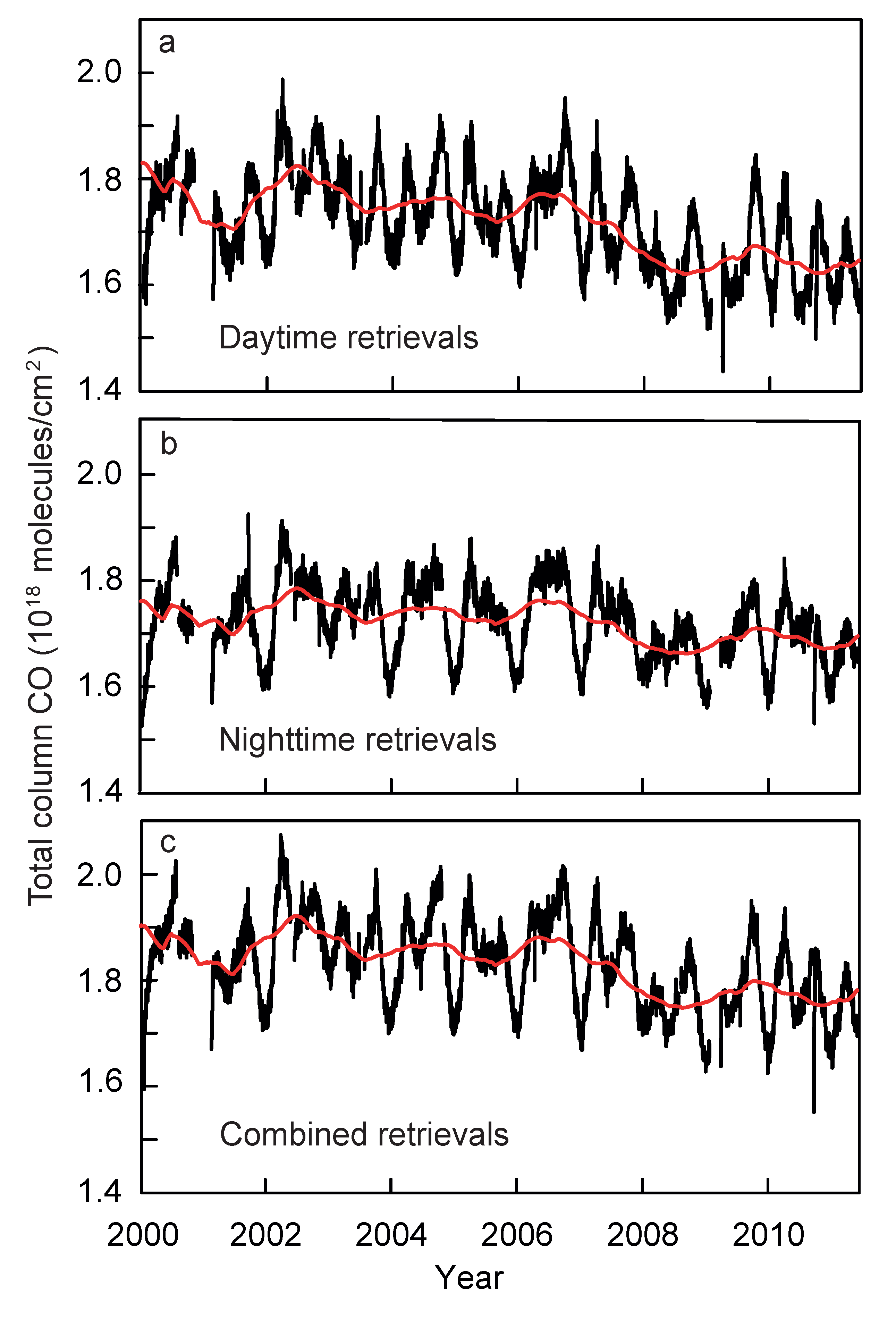
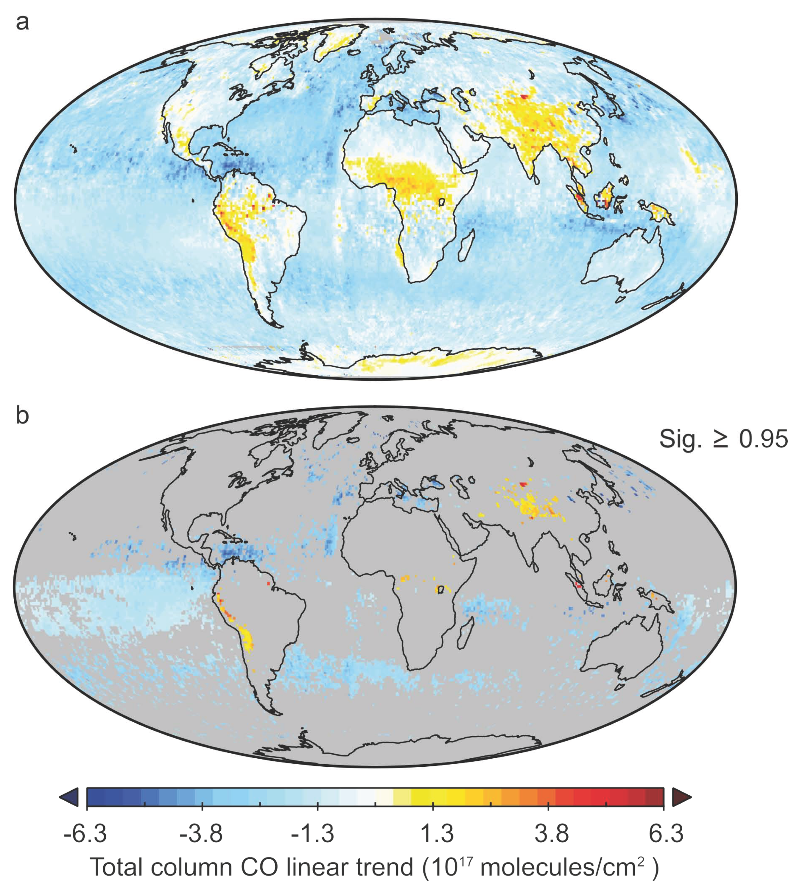
3.2. Trends in Tropospheric Carbon Monoxide: 2000–2012

Data compiled from ground-based measurement sites over the 1980s indicated CO was increasing at a rate of ∼1% per year [48,49]. However, continued monitoring showed significant reductions in CO emissions between 1980 to present, attributable to progressive improvements in vehicle efficiency and the implementation of catalytic converter technology [50,51]. Indeed, the globally-averaged combined retrievals shown in Figure 1c indicate that a statistically significant negative linear trend is present in the CO data between 2000–2012 of y = $-2.97$× 10${}^{13}$ x + 1.89 × 10${}^{18}$, r = $-0.42$, $p<0.01$ (degrees of freedom = 44): where the degrees of freedom (df) were estimated from the effective sample size of the data using the method of Neal [52] and Ripley [53]. The linear trend in the MOPITT data constitutes a globally-averaged CO reduction of 1.23 × 10${}^{17}$ molecules/cm${}^2$ over the March 2000–April 2012 period: equivalent to a net CO reduction of 6.85% (or 0.56% per year). We note the differences in the trends between daytime, nighttime, and combined retrievals in Figure 1 result from changes in instrumental sensitivity.

In Figure 3 we present an analysis of the long-term changes in CO, measured at each 1${}^{\circ }$ × 1${}^{\circ }$ pixel, between March 2000 and April 2012. For each pixel, the total column CO (combined) data are averaged into monthly values, and a linear regression is fitted to the resulting one-dimensional time-series. The long-term CO change was then calculated as the difference between the last and first values of the linear fit. In some instances we compensated for the presence of missing data by applying a linear interpolation to the time series where necessary: although if >50% of the data points were missing no interpolation was attempted, and the pixel was disregarded. The plot presented in Figure 3a shows the difference between the last and first point of the linear fits for the time-series of all successfully calculated pixels. In Figure 3b only data for pixels with a statistically significant ($p<0.05$) linear trend are shown. For these calculations, the assigned number of df for each pixel were calculated from the effective sample size.

Figure 3. Total column CO linear trends (10${}^{17}$ molecules/cm${}^2$) between March 2000 and April 2012 for: (a) the entire globe, and (b) statistically significant pixels ($p<0.05$).

Figure 3. Total column CO linear trends (10${}^{17}$ molecules/cm${}^2$) between March 2000 and April 2012 for: (a) the entire globe, and (b) statistically significant pixels ($p<0.05$).

MOPITT shows increasing CO trends over widespread regions of South America, Mexico, central Africa, Greenland, the eastern Antarctic, and the entire region of India and China. For virtually all other regions reductions in CO are observed. These negative trends are particularly prominent over northern middle latitude ocean regions, whereas the (less extensive) positive trends identified are restricted to land regions. Of the significant increases in CO, the changes are most intense over Eastern China (∼1.38 × 10${}^{15}$ molecules/cm${}^2$/year). While it is difficult to comment on the physical validity of these trends, it is likely that the positive trends are attributed to increased human activity, as similar significant increases in tropospheric pollution over China during the past decade have been widely reported from alternative sources (such as NO${}_x$ emissions), which have been found to be stable and reducing over Europe and North America while steadily increasing over Asia (e.g., [54,55,56,57]).

With regards to the comparatively weaker and more localized increases in total column CO observed over Africa and South America, biomass burning had previously been considered the primary factor influencing atmospheric pollution over such regions [58]. However, it is likely that the the observed CO increases of the past decade are attributable to increased economic growth, and may indicate a rise of major Southern Hemisphere contributors to atmospheric pollution, as suggested by Akimoto [54].

While significant localized increases in CO are observed over populated areas, for example over Eastern China (in the provinces of Xinjiang, Qinghai, Sichuan, and Tibet), some of the locally significant CO increases detected were situated in sparsely populated sites, such as the Gobi desert in Southern Mongolia/Northern China, and also along sparsely populated sites along the Western coast of South America. We speculate that the significant accumulation of CO in these regions may relate to local topography constraints on the horizontal transport of CO in the lower-troposphere [31].

It is known that MOPITT shows a positive measurement bias compared to in-situ CO observations, and that this bias is increasing over time due to instrumental drift [35,40,41]. Consequently, MOPITT has likely underestimated the decline in globally averaged total column CO over the past decade. While the magnitude of this underestimation may possibly be of the order of 20% according to validations from an earlier (version 4) MOPITT dataset [40], the long-term reliability of the version 5 data are improved [39].

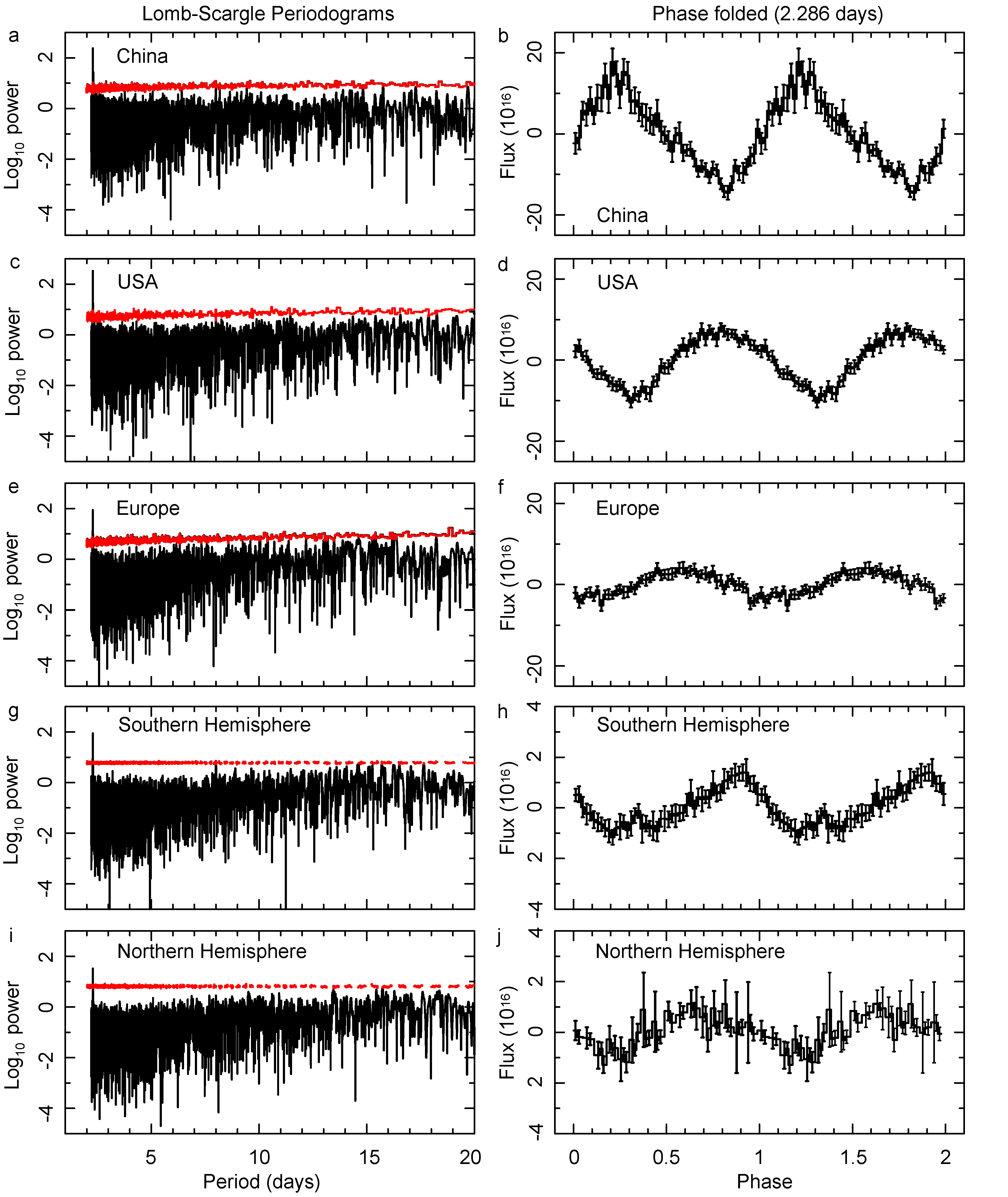
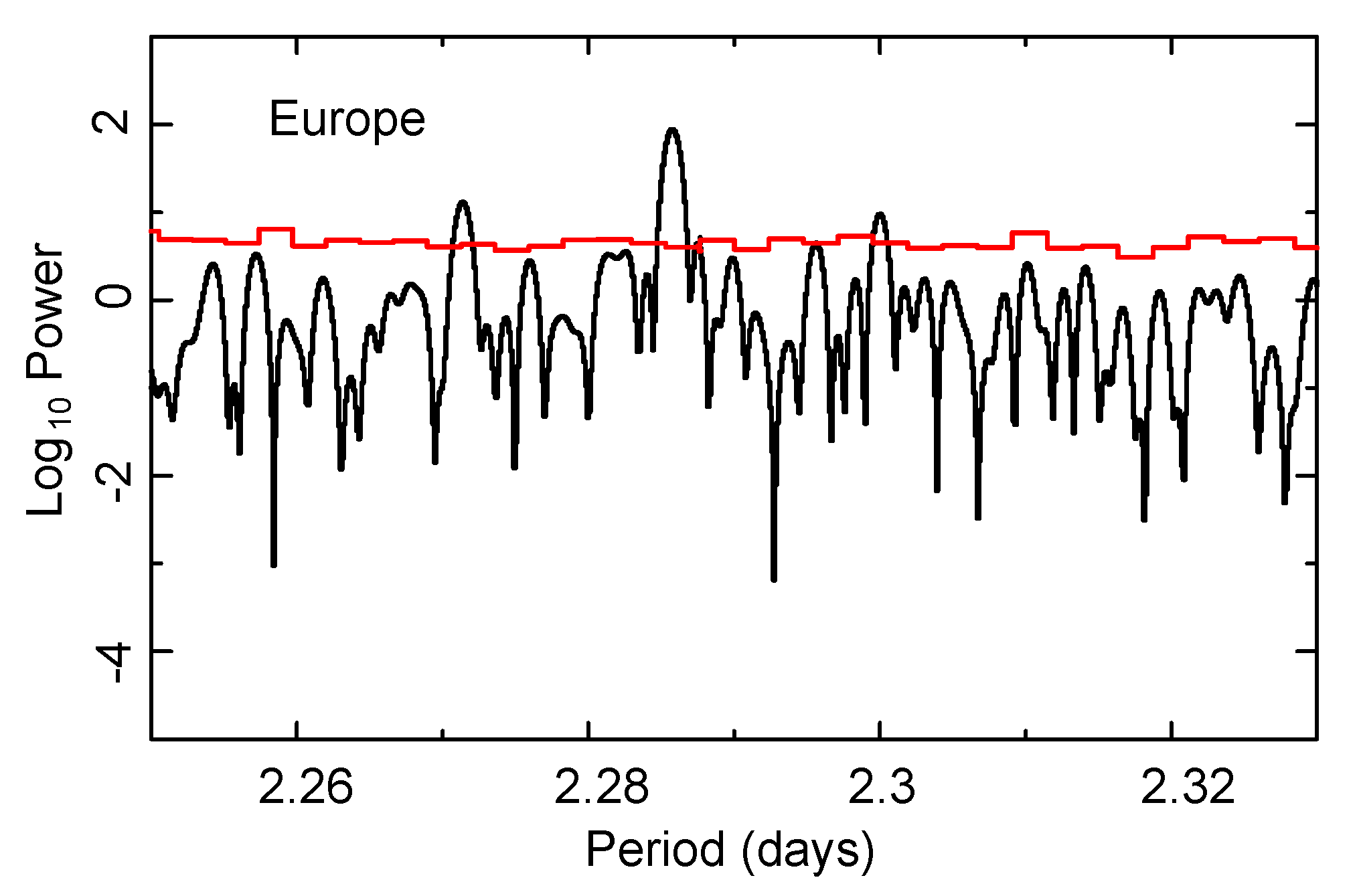
3.3. Period Analysis

We have identified several areas of the globe to examine independently for periodicities, these regions are as follows: China (75${}^{\circ }$E to 135${}^{\circ }$E, 20${}^{\circ }$N to 45${}^{\circ }$N), Europe ($-9$${}^{\circ }$E to 25${}^{\circ }$E, 35${}^{\circ }$N to 60${}^{\circ }$N), and the United States of America ($-68$${}^{\circ }$E to $-124$${}^{\circ }$E, 25${}^{\circ }$N to 48${}^{\circ }$N); only data over land is considered within these regions. In addition, we also examine the Northern (>0${}^{\circ }$N, 0–360${}^{\circ }$E) and Southern (<0${}^{\circ }$N, 0–360${}^{\circ }$E) hemispheres in their entirety. The use of regional scales is important, as although anthropogenic periods have been robustly identified at local scales, robustly detecting periodic, low-amplitude impacts of anthropogenic emissions in satellite-detected cloud properties at local scales with currently available datasets would be unlikely. To detect a low-amplitude signal in a dataset with a high level of spatio-temporal variability requires either a long observational period, averaging over a large-area, or both: as a result, we examine domains at a regional-scale.

We have applied the Lomb-Scargle period analysis [59,60] to the combined MOPITT data. The range of frequencies investigated was constrained using the limits imposed by the Nyquist frequency and the duration of the dataset, and the number of independent frequencies were determined using the method of Horne and Baliunas [61]. Prior to the analysis, the seasonal CO variations noted in Figure 2 were removed from the datasets by subtracting a 50-day smooth (running-mean) of the data from the daily values: consequently, the shortest period we could reliably identify begin at 2.0 days, while the longest are up-to 20 days. The resulting periodograms are shown in Figure 4.

Figure 4. Lomb-Scargle periodograms and 2.286 day phase folded data of MOPITT total column CO, averaged over: (a,b) China, (c,d) USA, (e,f) Europe, (g,h) the Northern Hemisphere, and (i,j) the Southern Hemisphere. The red lines indicate the Monte Carlo calculated significance thresholds at the $p<0.01$ (two-tailed) level. Statistically significant peaks in the power spectrum are found in all cases at 2.286 days.

Figure 4. Lomb-Scargle periodograms and 2.286 day phase folded data of MOPITT total column CO, averaged over: (a,b) China, (c,d) USA, (e,f) Europe, (g,h) the Northern Hemisphere, and (i,j) the Southern Hemisphere. The red lines indicate the Monte Carlo calculated significance thresholds at the $p<0.01$ (two-tailed) level. Statistically significant peaks in the power spectrum are found in all cases at 2.286 days.

In the periodograms the only clearly statistically significant peak in the spectrum occurs at a frequency of 0.4375 cycles/day (corresponding to a period of 2.286 days). The coherence, defined as the center frequency divided by the full width at half maximum (FWHM) of the peak, is >2,000 for all datasets and is consistent with a periodic modulation. The periodigrams are shown with corresponding phase folding plots, folded on to the 2.28 day period and binned into 50 phase bins. A clear modulation is evident, present not only at the regional scale in China, the USA, and Europe, but also across both the Northern and Southern hemispheres. For clarity, we present an expanded Lomb-Scargle plot focusing of the significant 2.286 day period, equivalent to Figure 4e, in Figure 5.

Figure 5. Lomb-Scargle periodogram of the European region, as shown in Figure 4e, focused on the statistically significant period centered around 2.286 days.

Figure 5. Lomb-Scargle periodogram of the European region, as shown in Figure 4e, focused on the statistically significant period centered around 2.286 days.

The standard false alarm probability estimate from the Lomb-Scargle algorithm gives the significance of the highest peak in the power spectrum assuming that all the data points are independent. However, in the presence of correlated data (i.e., red-noise), a different approach is needed in order to properly estimate the significance of the frequencies identified in the periodograms. We have done this numerically by means of Monte Carlo simulations. We simulated data with exactly the same sampling as the real MOPITT data, using a modeled red-noise data, and employing the method of Timmer and König [62] with a power-law as determined from the periodogram of the observed data. We then added Gaussian noise using the CO total column mean uncertainties from the MOPITT data. We then calculated the Lomb-Scargle periodograms and recorded the position and frequency of the highest peaks. We computed 10,000 randomized datasets using this methodology, and then calculated the 99% confidence levels at each frequency, taking into account a realistic number of independent trials [63]. In Figure 4 we display the resulting confidence levels over the periodograms: from these statistical evaluations, it is clear that the peak in the periodograms at 0.4375 cycles/day is significant above the 99% confidence level.

With the exception of the 2.28 day periodicity, we identified no statistically significant period in the total column CO data, existing between 1 and ∼20 days across the regions of China, the EU, or the USA: as a result we are unable to use regional scale data to examine the aerosol-indirect effect.

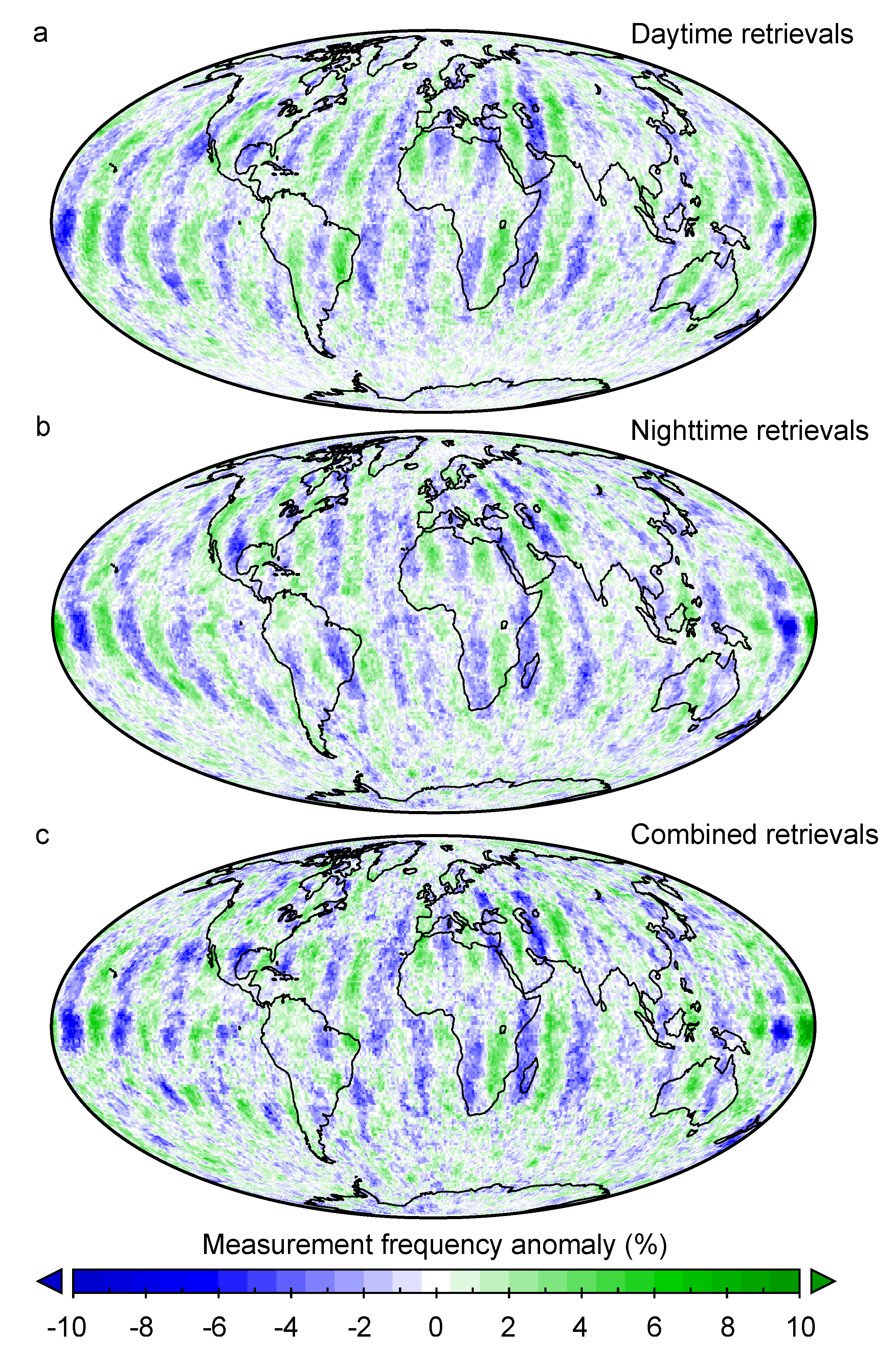
3.4. Periodic Changes in Measurement Frequency

We know of no physical process—anthropogenic or otherwise—that could account for a 2.28 day period being present in the CO data across the globe at both regional and hemispheric scales. The high coherence across the dataset suggests that the signal is most likely artificial in origin.

In order to further explore the origin of this period we have analyzed the difference in the number of observations made at each 1${}^{\circ }$ × 1${}^{\circ }$ pixel across the globe between the start and middle of the 2.28 day cycle (Figure 6). We find a very distinct distribution pattern, characteristic of the path of a polar orbiting satellite: we observe regular swath-shaped changes in measurement frequency across the globe of approximately ±10%. Additionally, these patterns are inclined in opposite directions between the daytime and nighttime retrievals—exactly as should be expected if these patterns are attributed to the path of a polar-orbiting satellite as it circumnavigates the globe from pole-to-pole. We note that the patterns also show some non-uniform noise. This is expected, as MOPITT data is only available for clear-sky conditions. Consequently, the noise is particularly prominent over regions that experience frequent cloud cover (e.g., Equatorial Africa, and the mid-to-high latitude Southern Hemisphere oceans).

Figure 6. Changes in MOPITT measurement signal (%) between the start and middle of the 2.28 day periodicity for (a) daytime, (b) nighttime, and (c) combined retrievals. Artificial shifts in sampling frequency of around 10% are observable over orbital tracks.

Figure 6. Changes in MOPITT measurement signal (%) between the start and middle of the 2.28 day periodicity for (a) daytime, (b) nighttime, and (c) combined retrievals. Artificial shifts in sampling frequency of around 10% are observable over orbital tracks.

This evidence suggests that the artificial cycle detected in the MOPITT data is the result of a regular variation in sampling frequency coupled with the spatially heterogeneous nature of the CO data (which is concentrated over centers of human activity): i.e., when more (fewer) measurements are taken from regions of relatively low (high) CO concentrations, it produces the impression that a fluctuation in regionally-averaged data has occurred. This effect creates a prominent ($p<0.01$) periodicity in the area-averaged CO data.

4. Conclusions

In order to investigate the indirect regional-scale impacts of emissions on clouds and climate we have attempted to identify anthropogenic periodicities in carbon monoxide data; this would indicate potential locations and periods to examine for evidence of indirect aerosol effects clearly distinguishable from natural variability. We examined several regional centers of human activity—China, the EU, and the USA—however, we found no clearly statistically significant period ($p<0.01$), with the exception of a 2.28 day signal. Not only was this signal present across all three regions, but it was also present when we considered data from the entire Northern and Souther hemispheres. Due to the spatial persistence and unexpected length of the period it is unlikely that it is due a physical change in carbon monoxide and associated anthropogenic emissions—consequently, we were unable to utilize these data as a means of examining the aerosol indirect effect. However, further examination of the data in relation to the 2.28 day periodicity indicated that the signal detected was artificial, related to the polar orbiting motion of the MOPITT instrument.

The significant periodicity in regional carbon monoxide data was essentially due to the MOPITT sensor repeatedly shifting back-and-fourth between areas of high and low concentrations of pollution. Consequently, the 2.28 day frequency appeared highly statistically significant. Similar sampling issues may also be present in other datasets with comparable spatio-temporal sampling from polar orbiting satellite data. These artifacts, however, may not be so easily detected in other datasets, as CO data is relatively unique in its temporal homogeneity yet spatial heterogeneity. We note that this artifact will only become problematic when sensitive measurements are needed at short timescales (<1 month) for data averaged over large regions (e.g., considering areas that span distances of more than one sensor-swath width).

References

1. Twomey, S. The influence of pollution on the shortwave albedo of clouds. J. Atmos. Sci. 1977, 34, 1149–1152. [Google Scholar] [CrossRef]
2. Platnick, S.; Twomey, S. Determining the susceptibility of cloud albedo to changes in droplet concentration with the Advanced Very High Resolution Radiometer. J. Appl. Meteorol. 1994, 33, 334–347. [Google Scholar] [CrossRef]
3. Lohmann, U.; Feichter, J. Global indirect aerosol effects: A review. Atmos. Chem. Phys. 2005, 5, 715–737. [Google Scholar] [CrossRef]
4. Solomon, S.; Qin, D.; Manning, M.; Chen, Z.; Marquis, M.; Averyt, K.; Tignor, M.; Miller, H. Climate Change 2007—The Physical Science Basis: Working Group I Contribution to the Fourth Assessment Report of the IPCC; Cambridge University Press: Cambridge, UK, 2007; Volume 4. [Google Scholar]
5. Cerveny, R.S.; Balling, R.C. Weekly cycles of air pollutants, precipitation and tropical cyclones in the coastal NW Atlantic region. Nature 1998, 394, 561–563. [Google Scholar] [CrossRef]
6. Graedel, T.E.; Farrow, L.A.; Weber, T.A. Photochemistry of the “Sunday Effect”. Environ. Sci. Technol. 1977, 11, 690–694. [Google Scholar] [CrossRef]
7. Karl, T. Day of the week variations of photochemical pollutants in the St. Louis area. Atmos. Environ. 1978, 12, 1657–1667. [Google Scholar] [CrossRef]
8. Jin, M.; Shepherd, J.M.; King, M.D. Urban aerosols and their variations with clouds and rainfall: A case study for New York and Houston. J. Geophys. Res. Atmos. 2005. [Google Scholar] [CrossRef]
9. Quaas, J.; Boucher, O.; Jones, A.; Weedon, G.; Kieser, J.; Joos, H. Exploiting the weekly cycle as observed over Europe to analyse aerosol indirect effects in two climate models. Atmos. Chem. Phys. 2009, 9, 8493–8501. [Google Scholar] [CrossRef]
10. Riga-Karandinos, A.; Saitanis, C.; Arapis, G. Study of the weekday-weekend variation of air pollutants in a typical Mediterranean coastal town. Int. J. Environ. Pollut. 2006, 27, 300–312. [Google Scholar] [CrossRef]
11. Forster, P.M.F.; Solomon, S. Observations of a weekend effect in diurnal temperature range. Proc. Natl. Acad. Sci. USA 2003, 100, 11225–11230. [Google Scholar] [CrossRef] [PubMed]
12. Bäumer, D.; Vogel, B. An unexpected pattern of distinct weekly periodicities in climatological variables in Germany. Geophys. Res. Lett. 2007. [Google Scholar] [CrossRef]
13. Tesouro, M.; de La Torre, L.; Nieto, R.; Gimeno, L.; Ribera, P.; Gallego, D. Weekly cycle in NCAR-NCEP reanalysis surface temperature data. Atmósfera 2005, 18, 205–209. [Google Scholar]
14. Sanchez-Lorenzo, A.; Calbó, J.; Martin-Vide, J. Reply to comment by HJ Hendricks Franssen et al. on “Winter ‘weekend effect’ in southern Europe and its connections with periodicities in atmospheric dynamics”. Geophys. Res. Lett. 2009. [Google Scholar] [CrossRef]
15. Gordon, A. Weekdays warmer than weekends? Nature 1994, 367, 325–326. [Google Scholar] [CrossRef]
16. Sitnov, S. Aerosol optical thickness and the total carbon monoxide content over the European Russia territory in the 2010 summer period of mass fires: Interrelation between the variation in pollutants and meteorological parameters. Izv. Atmos. Ocean. Phys. 2011, 47, 714–728. [Google Scholar] [CrossRef]
17. Sanchez-Lorenzo, A.; Laux, P.; Hendricks Franssen, H.J.; Calbó, J.; Vogl, S.; Georgoulias, A.; Quaas, J. Assessing large-scale weekly cycles in meteorological variables: A review. Atmos. Chem. Phys. 2012, 12, 5755–5771. [Google Scholar] [CrossRef]
18. Delisi, M.P.; Cope, A.M.; Franklin, J.K. Weekly precipitation Ccycles along the northeast corridor? Weather Forecast. 2001, 16, 343–353. [Google Scholar] [CrossRef]
19. Schultz, D.M.; Mikkonen, S.; Laaksonen, A.; Richman, M.B. Weekly precipitation cycles? Lack of evidence from United States surface stations. Geophys. Res. Lett. 2007. [Google Scholar] [CrossRef]
20. Choi, Y.S.; Ho, C.H.; Kim, B.G.; Hur, S.K. Long-term variation in midweek/weekend cloudiness difference during summer in Korea. Atmos. Environ. 2008, 42, 6726–6732. [Google Scholar] [CrossRef]
21. Givati, A.; Rosenfeld, D. Quantifying precipitation suppression due to air pollution. J. Appl. Meteorol. 2004, 43, 1038–1056. [Google Scholar] [CrossRef]
22. Zhao, C.; Tie, X.; Lin, Y. A possible positive feedback of reduction of precipitation and increase in aerosols over eastern central China. Geophys. Res. Lett. 2006. [Google Scholar] [CrossRef]
23. Ho, C.H.; Choi, Y.S.; Hur, S.K. Long-term changes in summer weekend effect over northeastern China and the connection with regional warming. Geophys. Res. Lett. 2009. [Google Scholar] [CrossRef]
24. Yum, S.S.; Cha, J.W. Suppression of very low intensity precipitation in Korea. Atmos. Res. 2010, 98, 118–124. [Google Scholar] [CrossRef]
25. Alpert, P.; Halfon, N.; Levin, Z. Does air pollution really suppress precipitation in Israel? J. Appl. Meteorol. Climatol. 2008, 47, 933–943. [Google Scholar] [CrossRef]
26. Stjern, C.W.; Stohl, A.; Kristjánsson, J.E. Have aerosols affected trends in visibility and precipitation in Europe? J. Geophys. Res. Atmos. 2011. [Google Scholar] [CrossRef]
27. Stjern, C. Weekly cycles in precipitation and other meteorological variables in a polluted region of Europe. Atmos. Chem. Phys. 2011, 11, 4095–4104. [Google Scholar] [CrossRef]
28. Ackerman, S.A. Remote sensing aerosols using satellite infrared observations. J. Geophys. Res. Atmos. 1997, 102, 17069–17079. [Google Scholar] [CrossRef]
29. Torres, O.; Bhartia, P.; Herman, J.; Sinyuk, A.; Ginoux, P.; Holben, B. A long-term record of aerosol optical depth from TOMS observations and comparison to AERONET measurements. J. Atmos. Sci. 2002, 59, 398–413. [Google Scholar] [CrossRef]
30. Conway, T.; Tans, P.; Waterman, L.; Thoning, K.; Masarie, K.; Gammon, R. Atmospheric carbon dioxide measurements in the remote global troposphere, 1981–1984. Tellus B 1988, 40, 81–115. [Google Scholar] [CrossRef]
31. Edwards, D.; Emmons, L.; Hauglustaine, D.; Chu, D.; Gille, J.; Kaufman, Y.; Pétron, G.; Yurganov, L.; Giglio, L.; Deeter, M.; et al. Observations of carbon monoxide and aerosols from the Terra satellite: Northern Hemisphere variability. J. Geophys. Res. 2004. [Google Scholar] [CrossRef]
32. Novelli, P.; Masarie, K.; Lang, P. Distributions and recent changes of carbon monoxide in the lower troposphere. J. Geophys. Res. Atmos. 1998, 103, 19015–19033. [Google Scholar] [CrossRef]
33. Pan, L.; Gille, J.C.; Edwards, D.P.; Bailey, P.L.; Rodgers, C.D. Retrieval of tropospheric carbon monoxide for the MOPITT experiment. J. Geophys. Res. Atmos. 1998, 103, 32277–32290. [Google Scholar] [CrossRef]
34. Fortems-Cheiney, A.; Chevallier, F.; Pison, I.; Bousquet, P.; Szopa, S.; Deeter, M.; Clerbaux, C. Ten years of CO emissions as seen from Measurements of Pollution in the Troposphere (MOPITT). J. Geophys. Res. Atmos. 2011. [Google Scholar] [CrossRef]
35. Deeter, M.; Worden, H.; Gille, J.; Edwards, D.; Mao, D.; Drummond, J.R. MOPITT multispectral CO retrievals: Origins and effects of geophysical radiance errors. J. Geophys. Res. 2011. [Google Scholar] [CrossRef]
36. Deeter, M.; Worden, H.; Edwards, D.; Gille, J.; Andrews, A. Evaluation of MOPITT retrievals of lower-tropospheric carbon monoxide over the United States. J. Geophys. Res. Atmos. (1984–2012) 2012. [Google Scholar] [CrossRef]
37. Deeter, M.; Emmons, L.; Edwards, D.; Gille, J.; Drummond, J.R. Vertical resolution and information content of CO profiles retrieved by MOPITT. Geophys. Res. Lett. 2004. [Google Scholar] [CrossRef]
38. Pan, L.; Edwards, D.P.; Gille, J.C.; Smith, M.W.; Drummond, J.R. Satellite remote sensing of tropospheric CO and CH(4): Forward model studies of the MOPITT instrument. Appl. Opt. 1995, 34, 6976–6988. [Google Scholar] [CrossRef] [PubMed]
39. Deeter, M.; Martínez-Alonso, S.; Edwards, D.; Emmons, L.; Gille, J.; Worden, H.; Pittman, J.; Daube, B.; Wofsy, S. Validation of MOPITT Version 5 thermal-infrared, near-infrared, and multispectral carbon monoxide profile retrievals for 2000–2011. J. Geophys. Res. Atmos. 2013. [Google Scholar] [CrossRef]
40. Emmons, L.; Edwards, D.; Deeter, M.; Gille, J.; Campos, T.; Nédélec, P.; Novelli, P.; Sachse, G. Measurements of Pollution in the Troposphere (MOPITT) validation through 2006. Atmos. Chem. Phys. 2009, 9, 1795–1803. [Google Scholar] [CrossRef]
41. Deeter, M.; Edwards, D.; Gille, J.; Emmons, L.; Francis, G.; Ho, S.P.; Mao, D.; Masters, D.; Worden, H.; Drummond, J.R.; et al. The MOPITT version 4 CO product: Algorithm enhancements, validation, and long-term stability. J. Geophys. Res. Atmos. 2010. [Google Scholar] [CrossRef]
42. Goldsmith, J.R.; Landaw, S.A. Carbon monoxide and human health. Science 1968, 162, 1352–1359. [Google Scholar] [CrossRef] [PubMed]
43. Hansen, A.B.; Palmgren, F. VOC air pollutants in Copenhagen. Sci. Total Environ. 1996, 189, 451–457. [Google Scholar] [CrossRef]
44. Nielsen, T. Traffic contribution of polycyclic aromatic hydrocarbons in the center of a large city. Atmos. Environ. 1996, 30, 3481–3490. [Google Scholar] [CrossRef]
45. Marr, L.C.; Harley, R.A. Modeling the effect of weekday-weekend differences in motor vehicle emissions on photochemical air pollution in central California. Environ. Sci. Technol. 2002, 36, 4099–4106. [Google Scholar] [CrossRef] [PubMed]
46. Ketzel, M.; Wåhlin, P.; Berkowicz, R.; Palmgren, F. Particle and trace gas emission factors under urban driving conditions in Copenhagen based on street and roof-level observations. Atmos. Environ. 2003, 37, 2735–2749. [Google Scholar] [CrossRef]
47. Khalil, M.; Rasmussen, R. The global cycle of carbon monoxide: Trends and mass balance. Chemosphere 1990, 20, 227–242. [Google Scholar] [CrossRef]
48. Khalil, M.; Rasmussen, R. Carbon monoxide in the Earth’s atmosphere: Increasing trend. Science 1984, 224, 54–56. [Google Scholar] [CrossRef] [PubMed]
49. Khalil, M.; Rasmussen, R. Carbon monoxide in the Earth’s atmosphere: Indications of a global increase. Nature 1988, 332, 242–245. [Google Scholar] [CrossRef]
50. Novelli, P.C.; Masarie, K.A.; Tans, P.P.; Lang, P.M. Recent changes in atmospheric carbon monoxide. Science 1994, 263, 1587–1590. [Google Scholar] [CrossRef] [PubMed]
51. Mott, J.A.; Wolfe, M.I.; Alverson, C.J.; Macdonald, S.C.; Bailey, C.R.; Ball, L.B.; Moorman, J.E.; Somers, J.H.; Mannino, D.M.; Redd, S.C. National vehicle emissions policies and practices and declining US carbon monoxide–related mortality. JAMA 2002, 288, 988–995. [Google Scholar] [CrossRef] [PubMed]
52. Neal, R.M. Probabilistic Inference Using Markov Chain Monte Carlo Methods; Technical Report CRG-TR-93-1; Department of Computer Science, University of Toronto: Toronto, Canada, 1993; pp. 1–144. [Google Scholar]
53. Ripley, B.D. Stochastic Simulation; Wiley: New York, NY, USA, 2009; Volume 316. [Google Scholar]
54. Akimoto, H. Global air quality and pollution. Science 2003, 302, 1716–1719. [Google Scholar] [CrossRef] [PubMed]
55. Richter, A.; Burrows, J.P.; Nüß, H.; Granier, C.; Niemeier, U. Increase in tropospheric nitrogen dioxide over China observed from space. Nature 2005, 437, 129–132. [Google Scholar] [CrossRef] [PubMed]
56. He, Y.; Uno, I.; Wang, Z.; Ohara, T.; Sugimoto, N.; Shimizu, A.; Richter, A.; Burrows, J.P. Variations of the increasing trend of tropospheric NO2 over central east China during the past decade. Atmos. Environ. 2007, 41, 4865–4876. [Google Scholar] [CrossRef]
57. Zhang, X.; Zhang, P.; Zhang, Y.; Li, X.; Qiu, H. The trend, seasonal cycle, and sources of tropospheric NO2 over China during 1997–2006 based on satellite measurement. Sci. China Ser. D Earth Sci. 2007, 50, 1877–1884. [Google Scholar] [CrossRef]
58. Edwards, D.; Emmons, L.; Gille, J.; Chu, A.; Attié, J.L.; Giglio, L.; Wood, S.; Haywood, J.; Deeter, M.; Massie, S.; et al. Satellite-observed pollution from Southern Hemisphere biomass burning. J. Geophys. Res. 2006. [Google Scholar] [CrossRef]
59. Scargle, J.D. Studies in astronomical time series analysis. IIStatistical aspects of spectral analysis of unevenly spaced data. Astrophys. J. 1982, 263, 835–853. [Google Scholar] [CrossRef]
60. Press, W.H.; Teukolsky, S.A.; Vetterling, W.T.; Flannery, B.P. Numerical Recipes in C: The Art of Scientific Computing; Cambridge University Press: Cambridge, UK, 1992. [Google Scholar]
61. Horne, J.H.; Baliunas, S.L. A prescription for period analysis of unevenly sampled time series. Astrophys. J. 1986, 302, 757–763. [Google Scholar] [CrossRef]
62. Timmer, J.; König, M. On generating power law noise. Astron. Astrophys. 1995, 300, 707–710. [Google Scholar]
63. Vaughan, S. A simple test for periodic signals in red noise. Astron. Astrophys. 2005, 431, 391–403. [Google Scholar] [CrossRef]