Simulated Regional Yields of Spring Barley in the United Kingdom under Projected Climate Change

Abstract

This paper assessed the effect of projected climate change on the grain yield of barley in fourteen administrative regions in the United Kingdom (UK). Climate data for the 2030s, 2040s and 2050s for the high emission scenario (HES), medium emissions scenario (MES) and low emissions scenario (LES) were obtained from the UK Climate Projections 2009 (UKCP09) using the Weather Generator. Simulations were performed using the AquaCrop model and statistics of simulated future yields and baseline yields were compared. The results show that climate change could be beneficial to UK barley production. For all emissions scenarios and regions, differences between the simulated average future yields (2030s–2050s) and the observed yields in the baseline period (1961–1990) ranged from 1.4 to 4 tons·ha⁻¹. The largest increase in yields and yield variability occurred under the HES in the 2050s. Absolute increases in yields over baseline yields were substantially greater in the western half of the UK than in the eastern regions but marginally from south to north. These increases notwithstanding, yield reductions were observed for some individual years due to saturated soil conditions (most common in Wales, Northern Ireland and South-West Scotland). These suggest risks of yield penalties in any growing season in the future, a situation that should be considered for planning adaptation and risk management.

1. Introduction

Barley (Hordeum vulgare L.) is widely grown due to its tolerance to a wide range of growing conditions. In terms of quantity of grains produced, barley is the fourth most important crop in the world [1]. In the United Kingdom (UK), barley is the second most widely grown arable crop (after wheat) and the number one crop in Scotland [2]. Feed use and malting account for over 60% and a little over 30%, respectively, of barley produced in the UK [2]. Premium whiskey and malt barley production confers a cultural significance to barley in the UK.

Climate change presents both opportunities and threats to barley production in the world. In northern temperate environments such as the UK, elevated atmospheric CO₂, together with moderate warming and adequate soil water supply, can be beneficial to a C₃ cereal crop like barley [3,4,5,6]. Such benefits include increased photosynthetic capacity, through radiation and water use efficiency, and thereby increased biomass production and harvest index [5,7,8,9,10,11,12,13,14,15,16]. With regard to threats, barley is sensitive to soil water and temperature regimes around establishment, anthesis and grain filling [17,18]. While barley is known to be moderately tolerant to soil water deficit [19], it is sensitive to anoxic conditions and heat stress, and compensates poorly with respect to reduced tillering in early stages. For example, simulation results show that intra-seasonal water deficits can reduce barley grain yields by up to 4.5 tons·ha⁻¹ in the 2050s in Ireland [14]. Warmer conditions can also hasten phenophases and senescence of barley and thereby reduce harvest index [18,20]. Thus, a combination of water and heat stress can potentially reduce the grain yield of barley in the UK.

Crop simulation models can be used to estimate the effects of climate change on crops. Crop simulation models vary in complexity and data requirements depending on the nature of their growth models [21]. Crop models used previously to assess the impact of projected climate change scenarios on barley include CERES–Barley [14,22,23,24,25], CropSyst [26,27], WOFOST [3,28]. While these models perform well, they are data-intensive. An evaluation of nine crop growth models for simulating spring barley yields in different climatic zones of Northern and Central Europe showed WOFOST as one of the top three performing models, with CropSyst showing large uncertainty [29]. Water-driven models, such as AquaCrop, (in which crop growth is mainly driven by water productivity and limited by soil water deficit) are now widely used because they are relatively simple, easy to use and less data intensive [30]. An evaluation of AquaCrop, CropSyst and WOFOST models under different soil water regimes showed comparable results [30]. In the current study, we used the AquaCrop model [31] because, although it has not been widely used in climate change studies, it is less data-intensive and its performance compares well with commonly used models. Moreover, it performed well during a calibration study involving three models and nine barley genotypes under Scottish conditions [32].

In the UK, precipitation generally decreases from West to East and North to South while the reverse is true for temperature. This suggests that climate change can have geographically different effects on barley production in the UK as observed in Ireland [14]. However, there is little information on the effects of climate change on barley grain yields at regional scale in the UK. Such information is relevant for planning adaptation at the regional level. The study reported in this paper, therefore, simulated the effect of projected climate change on barley grain yields across fourteen (14) administrative regions of the UK (Figure 1) in the 2030s, 2040s and 2050s.

2. Materials and Methods

2.1. Data Sources

2.1.1. Climate Data

The UK Climate Projections 2009 (UKCP09) is a database on probabilistic projected climate change over the UK [33]. The Weather Generator (WG, version 2) embedded in the UKCP09 [34] was used to generate future daily climate data for the 2030s, 2040s and 2050s under the high emissions scenario (HES), medium emissions scenario (MES) and low emissions scenario (LES) for each of the fourteen regions of the UK. The WG randomly samples a specified number of model variants from the probabilistic projections and uses a stochastic process to generate statistically credible future climate variables at 5 km grid resolution and at daily or hourly scales (see [34] for a detailed description).

Daily weather data for each region, time slice and emissions scenario was obtained by submitting appropriate request for standard WG variables to the UKCP09 database. For each request, 40 contiguous cells (maximum allowed) were selected in the region of interest based on the arable areas in the UK land cover map (LCM 2007, Centre for Ecology and Hydrology). Each WG run was 30 years and 100 random samples were requested from 10,000 randomly sampled model variants. From the output files generated by the WG for each request, climatic variables relevant for the simulations were extracted into a separate text file, using a Python code, for further processing to make them readable in the software for the simulations (AquaCrop).

The projected atmospheric CO₂ concentrations for the MES and LES were already in AquaCrop [31]. The projected atmospheric CO₂ concentration for the HES was created from data obtained from the IPCC data distribution centre (www.ipcc-data.org/ancillary/tar-isam.txt). “A future without climate change” scenario was not considered in the current study because of the medium-term warming effect of greenhouse gases already committed to the atmosphere and the current levels of greenhouse gas emissions [35,36,37].

2.1.2. Soil Data

Soil data was obtained from the Crop Growth Monitoring System (CGMS) database in the New Soil Information System (SINFO) [38]. The SINFO is part of the European Union programme on Monitoring Agriculture with Remote Sensing (MARS) Crop Yield Forecasting System (MCYFS, [38]). The SINFO database has a scale of 1:1,000,000 in which Europe is divided into soil mapping units (SMU). Each SMU has several soil typological units (STUs) with attributes describing the properties of the soils.

The SINFO data was downloaded and imported into ArcGIS 9.1 (ESRI™, Redlands, CA, USA) for further processing. The UK was clipped from the map and attribute tables were joined based on common fields. The SMU attribute table was joined to the STU attribute table using the common field smu no. and the resulting table was in turn joined to the soil physical group table via the common field soil group no. This resulted in one attribute table for all the soil polygons. The final map, with the joined table containing all the attributes for all the soil polygons, was exported to represent the UK soils used in the simulation. The UK soils map was intersected with a map of UK regions to obtain the distribution of soils in each region. For each region, the soil with the largest spatial distribution in arable areas was considered to be the dominant soil class. The weighted averages of the hydraulic attribute values of the dominant soil polygons were then used to represent the hydraulic properties of the soil for that region in the simulations.

2.1.3. Baseline Yield Data

The Home Grown Cereals Association (HGCA) Recommended List shows that the genotype Westminster is widely grown in the UK both as a spring and winter barley crop, for feed and malt, and is high-yielding. The genotype “Westminster” was used as the representative barley crop for the simulations. It was one of ten barley genotypes grown under Scottish conditions and used for a calibration study using the AquaCrop model (see [32]). Average barley yields for the baseline period (1961–1990) were obtained from the respective National Agricultural Statistics Departments in the UK. The data were harmonized in terms of units. For England, the regional yield data were available for the period 1999–2010. However, UK national yield data were available for the entire baseline period. The averages of the differences between the UK and each English regional yield for the period 1999 to 2010 were calculated. To obtain the yield for each English region for the baseline period, the average calculated above was subtracted from the UK national yield for the years in the baseline period. The same approach was used to fill gaps in the data for Northern Ireland.

2.2. Simulations

The AquaCrop model was used to simulate future yields of spring barley in the UK, using the calibration information on the genotype Westminster (see [32]), together with information from [31]. AquaCrop is a crop-water productivity model for simulating biomass production and yield response to soil water dynamics and climatic conditions [31,39]. It incorporates current knowledge of crop physiological responses to predict attainable yield of a crop. It is designed to offer a balance between accuracy, simplicity and robustness. The conceptual framework, underlying principles, and distinctive components and features of AquaCrop have been described by Steduto et al. [39]. The structural details and algorithms of AquaCrop have also been reported by Raes et al. [31].

The soil sub-model is designed as a dispersed system permitting the user to define up to five layers of varying textures and depths in the soil profile. This sub-model contains default values of hydraulic properties (saturated hydraulic conductivity, saturated water content, field capacity and wilting point), generated using a pedotransfer function, for all the soil textural classes defined in the USDA soil texture triangle. However, user-defined soil type and or values of hydraulic characteristics are permitted. The available soil water in the root zone is tracked from water input by performing a daily water balance that includes the processes of runoff, infiltration, redistribution, deep percolation, capillary rise, uptake, evaporation and transpiration. In performing soil water balance, AquaCrop separates soil evaporation from crop transpiration.

The crop-growth sub-model relies on the conservative behaviour of water productivity. Thus, biomass production in AquaCrop is a function of water productivity and crop transpiration relative to the extent of canopy cover. The canopy cover (expressed as a fraction of green canopy ground cover) is crucial as it determines the scale of transpiration and biomass production through its expansion, ageing, stomata conductance and senescence. Under unstressed conditions, canopy expansion from emergence to full cover follows an exponential growth function while the phase from full canopy to senescence follows a decay function. Subsequent to full canopy cover, the canopy can have a variable duration period prior to senescence. Lower level or intermediary processes of biomass accumulation are not simulated but synthetically incorporated into a single coefficient defined as biomass water productivity (WP), which is normalised for reference evapotranspiration (ET_O) and CO₂ concentration of the bulk atmosphere. This normalisation makes the model applicable to varied locations and seasons, including climate change scenarios. Even though the final yield is a product of biomass and harvest index (HI), AquaCrop separates final yield into biomass and HI and, thus, allows a distinction of environmental effects on biomass production and harvest index [31,40]. The crop-growth sub-model has five main components and related dynamic responses to environmental conditions (phenology, canopy cover, rooting depth, biomass production and harvest index). Crop responses to water stress occur through three main conservative, plant-based parameters: reduced rate of canopy expansion, stomatal control of transpiration, and accelerated canopy senescence [31,41]. Through these pathways, the WP and HI are adjusted. Other water stresses (e.g., waterlogging) can also affect the WP and HI. The stress functions of the crop responses are considered conservative with respect to management or geographical location, but the onset and intensity of stresses are strongly dependent on management, time, climate, and soil conditions [31]. Simulations can be run in either growing degree days or calendar days depending on data availability and user preference.

The HGCA indicates that the optimum sowing dates for spring barley range from late January to end February in the south and east of England and from late February to the end of March in Scotland. According to the HGCA, sowing outside the optimum period can result in a reduction in grain quality and yield penalties of 30–50 kg·ha⁻¹·day⁻¹. Hence, the search for appropriate sowing dates in the AquaCrop model was restricted to the HGCA recommended sowing period (±1 week). In AquaCrop, the sowing date for each region was obtained by forcing the model to the 1990 yield for that region by varying only the sowing date until the simulated yield approximated the observed yield [42]. The first sowing date that gave the closest match between the simulated and observed yields was used as the sowing date [42]. The differences between the observed and simulated yields for 1990 ranged from −0.14 to 0.59 tons·ha⁻¹. To compensate for yield increase due to, for example, genetic improvement, the reference harvest index (HIo) was reduced to 0.46 when the model was being forced to the 1990 baseline. This is because using a HIo of 0.49 gave yields substantially higher than the actual yields. The HIo was restored to 0.49 for the climate change simulations. The reliability of the sowing dates and the model setup were assessed by comparing simulated and observed yields for the period 1980–1989 [42] using the root mean square error (RMSE, [43]):

$$RMSE(\%)={\displaystyle \sum }_{i=1}^n\sqrt{\left[\frac{{(P_i-O_i)}^2}{n}\right]}\times \frac{100}{m}$$

where P_i and O_i are the predicted and observed yields, respectively; n and m are the number of observations and the mean of the observed yields, respectively.

Fertility stress and irrigation were not considered for any of the simulations. Furthermore, no field management was specified and the initial soil water content was set to field capacity. The main parameters used in AquaCrop for the simulations are presented in

Table 1. AquaCrop parameters used in the simulations.

Symbol	Parameter Description	Value
1. Crop Phenology
1.1. Development of green canopy cover (CC)
Tbase	Base temperature (°C)	0
Tupper	Upper temperature (°C)	22
	Initial canopy cover (%)	3.6
	Time from sowing to emergence (GDD)	135
	Canopy growth coefficient (fraction per GDD)	0.8
	Maximum canopy cover (%)	85
	Time from sowing to flowering (GDD)	950
	Length of flowering stage (GDD)	215
	Time from sowing to start of senescence (GDD)	1315
	Canopy decline coefficient (fraction per GDD)	0.06
	Time from sowing to maturity (GDD)	1675
1.2. Development of root zone
	Minimum effective rooting depth (m)	0.30
	Maximum effective rooting depth (m)	0.70
	Shape factor describing root zone expansion	1.5
2. Crop Transpiration
	Crop coefficient at maximum CC	1.15
	Decline of crop coefficient (%·day−1) due to ageing	0.15
	Effect of canopy shelter on surface evaporation in late season stage (%)	50
3. Biomass production and yield formation
3.1. Crop water productivity
WP*	Water productivity normalized for ETO and CO2 (g·m−2)	15
	Water productivity normalized for ETO and CO2 during yield formation (as % WP* before yield formation)	100
3.2. Harvest index (HI)
	Reference harvest index (HIo)	0.49
	Upper threshold for water stress during flowering on HI	0.82
	Possible increase (%) of HI due to water stress before flowering	12 (strong)
	Coefficient describing positive effect of restricted vegetative growth during yield formation on HI	Moderate
	Coefficient describing negative effect of stomatal closure during yield formation on HI	Moderate
	Excess of potential fruits	Moderate
	Allowable maximum increase (%) of specified HI	15
4. Stresses
4.1. Soil water stress
Pexp,lower	Lower threshold of water stress for triggering inhibited canopy expansion	0.60
Pexp,upper	Upper threshold for canopy expansion (canopy expansion seizes)	0.27
	Shape factor for water stress coefficient for canopy expansion	3.5
Psto	Upper threshold for stomata closure	0.60
	Shape factor for water stress coefficient for stomatal control	3.0
Psen	Upper threshold for early senescence due to water stress	0.60
	Shape factor for water stress coefficient for canopy senescence	3.5
Ppol	Upper threshold of soil water depletion for failure of pollination	0.80
	Vol. % at anaerobiotic point (with reference to saturation)	15
4.2. Temperature stress
	Minimum air temperature below which pollination starts to fail (cold stress, °C)	5
	Maximum air temperature above which pollination starts to fail (heat stress, °C)	30
	Minimum growing degrees required for full biomass production (°C-day)	15

. Using the relevant climate, soil and crop files, 100 multiple run project files were created for each region, time slice and emissions scenario. The multiple run project files were transferred to the AquaCrop plug-in program [31] in which the simulations were executed.

2.3. Data Analysis

The output text files of the climate change simulations for each of the 100 multiple run project files for each region, time slice and emissions scenario were imported to separate worksheets in a Microsoft Excel 2010 workbook. Descriptive statistics, including percentiles, were then computed for the simulated yields for each time slice, emissions scenario and region using the Data Analysis tool. The same computation was done for the baseline yield data. Differences between projected yields and observed yields in the baseline period were calculated. Temporal trends in yields in both the baseline and future climates were generated and causes of yield dips were explored.

3. Results

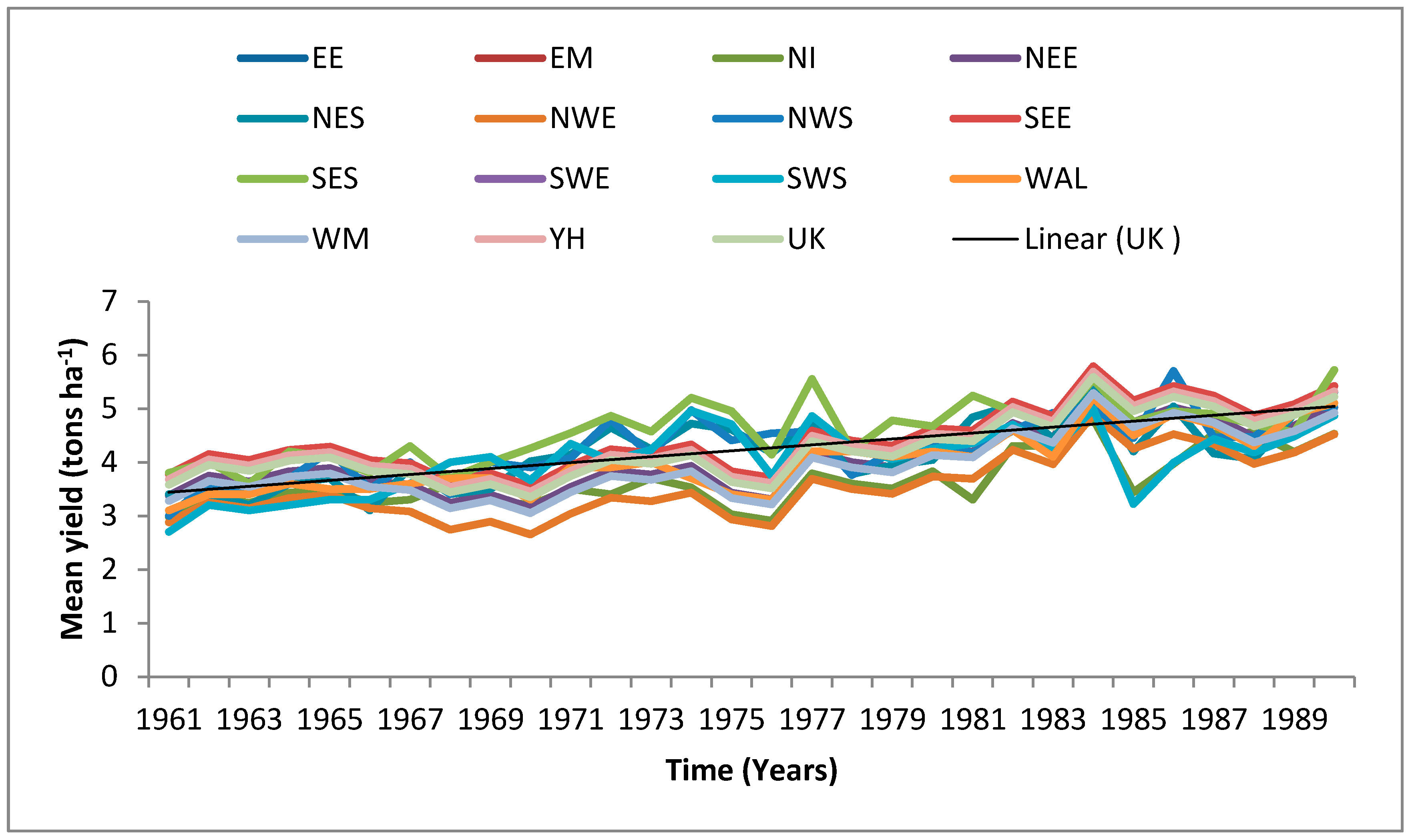
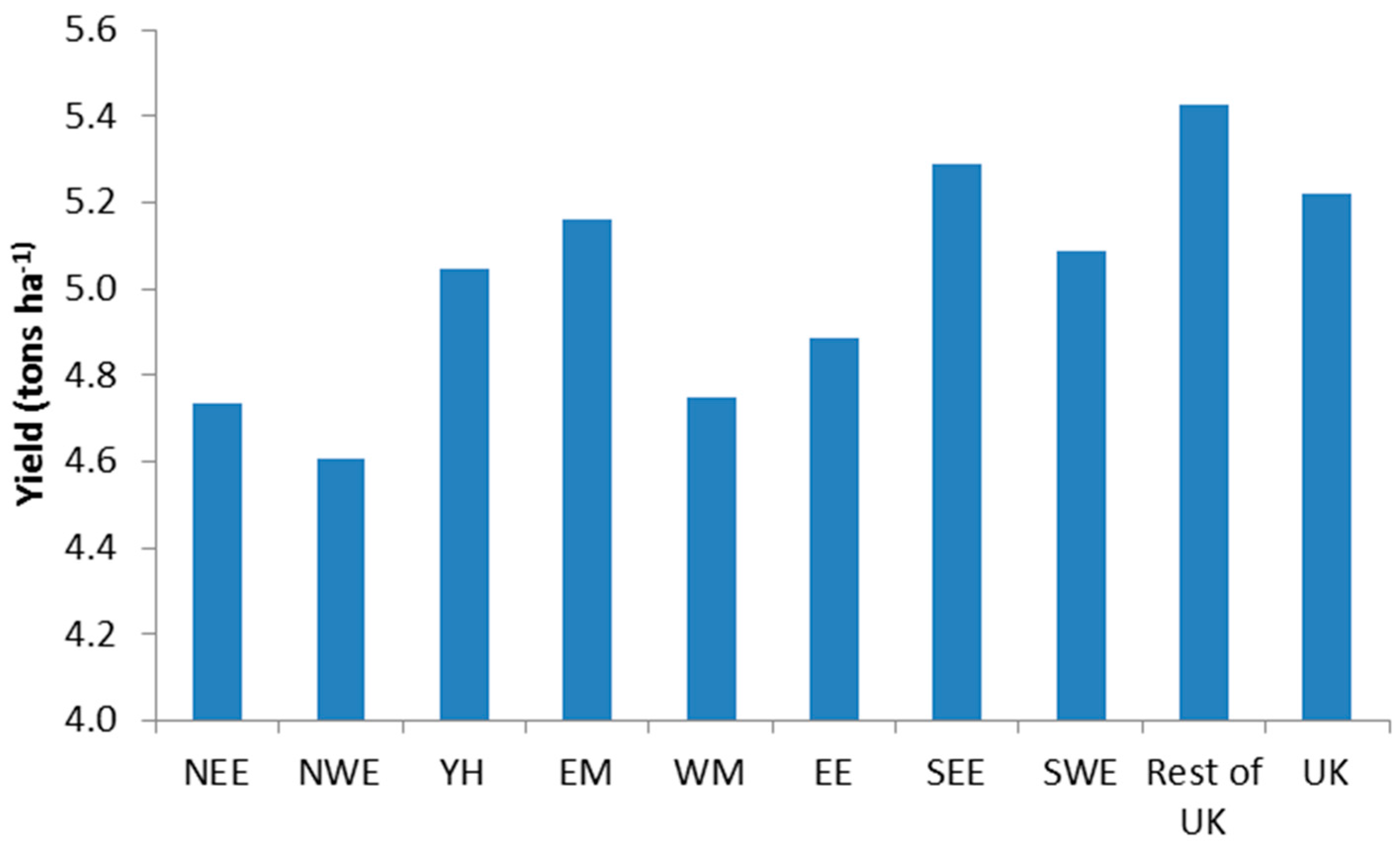
3.1. Baseline Yields

Mean yields for the baseline period ranged from approximately 3.7 tons·ha⁻¹ in Northern Ireland (NI) to 4.6 tons·ha⁻¹ in South East Scotland (SES), with a UK average of 4.2 tons·ha⁻¹ (

Table 2. Descriptive statistics of observed yields for the baseline period (1960–1990).

Statistic	Mean	Max.	90th Perc.	Median	10th Perc.	Min.	Std. Error	Std. Dev.	Skewness
EE	4.34	5.69	5.14	4.20	3.68	3.45	0.11	0.60	0.54
EM	4.34	5.69	5.14	4.20	3.68	3.45	0.11	0.60	0.54
NI	3.66	4.80	4.53	3.51	3.20	2.91	0.09	0.51	0.75
NEE	4.04	5.39	4.84	3.90	3.38	3.15	0.11	0.60	0.54
NES	4.19	5.43	5.04	4.15	3.40	3.10	0.12	0.64	0.17
NWE	3.54	4.89	4.34	3.40	2.88	2.65	0.11	0.60	0.54
NWS	4.28	5.70	5.01	4.27	3.50	3.00	0.11	0.60	0.06
SEE	4.44	5.79	5.24	4.30	3.78	3.55	0.11	0.60	0.54
SES	4.57	5.72	5.24	4.62	4.00	3.60	0.10	0.56	0.18
SWE	3.94	5.29	4.74	3.80	3.28	3.05	0.11	0.60	0.54
SWS	4.03	4.99	4.86	4.14	3.22	2.70	0.11	0.62	−0.35
WAL	4.00	5.20	4.90	3.95	3.40	3.10	0.10	0.58	0.51
WM	3.94	5.29	4.74	3.80	3.28	3.05	0.11	0.60	0.54
YH	4.34	5.69	5.14	4.20	3.68	3.45	0.11	0.60	0.54
UK	4.24	5.59	5.04	4.10	3.58	3.35	0.11	0.60	0.54

Note: Max., Min. are maximum and minimum respectively; Perc. is percentile; Std. is standard; EE (Eastern England), EM (East Midlands), NI (Northern Ireland), NEE (North East England), NES (North East Scotland), NWE (North West England), NWS (North West Scotland), SEE (South East England), SES (South East Scotland), SWE (South West England), SWS (South West Scotland), WAL (Wales), WM (West Midlands), YH (Yorkshire and Humber).

). Six regions had mean yields greater than the UK yield. The 90th percentiles ranged from 4.3 tons·ha⁻¹ in North West England (NWE), to 5.2 tons·ha⁻¹ in South East England (SEE) and South East Scotland (SES), while the 10th percentiles ranged from 2.9 to 4.0 tons·ha⁻¹. Generally, the baseline yields increased marginally from west to east and from south to north. The standard deviations were low and the differences between regional yields were not substantial. The regional yields were positively skewed (except South West Scotland, SWS) but the low skewness values indicate that few yield values exceeded their respective mean yield values. Figure 2 shows low temporal variation in the baseline yields for all the regions, suggesting yield stability over time. The baseline yields also showed an increasing trend over time.

To provide a perspective, the 2010 spring barley yields of English regions are presented in Figure 3. The yields ranged from 4.6 tons·ha⁻¹ (NWE) to 5.3 tons·ha⁻¹ (SEE) (Figure 3). The mean yield for the English regions was 4.9 tons·ha⁻¹. The mean yield for the rest of the UK (Wales, Northern Ireland and Scotland) was 5.4 tons·ha⁻¹ and the UK average was 5.2 tons·ha⁻¹.

3.2. Accuracy of Sowing Dates

The sowing dates ranged from February 13 for Eastern England (EE) to March 24 for North West Scotland (NWS) (

Table 3. Sowing dates used in the simulations for UK regions and their associated accuracies.

Region	Sowing Date	Root Mean Square Error (RMSE)
EE	13 February	0.44
EM	27 February	0.79
NI	8 March	0.66
NEE	7 March	0.68
NES	9 March	0.74
NWE	19 February	0.74
NWS	24 March	0.81
SEE	24 February	0.55
SES	9 March	0.55
SWE	17 February	0.65
SWS	13 March	0.73
WA	19 February	1.15
WM	27 February	0.73
YH	27 February	0.78
UK	-	0.35

). The RMSE values associated with the sowing dates and model parameters ranged from 0.44 (EE) to 1.15 tons·ha⁻¹ (Wales, WA) and 0.35 tons·ha⁻¹ for the UK. It is noteworthy that the regional average yields are a mix of different genotypes under different management practices.

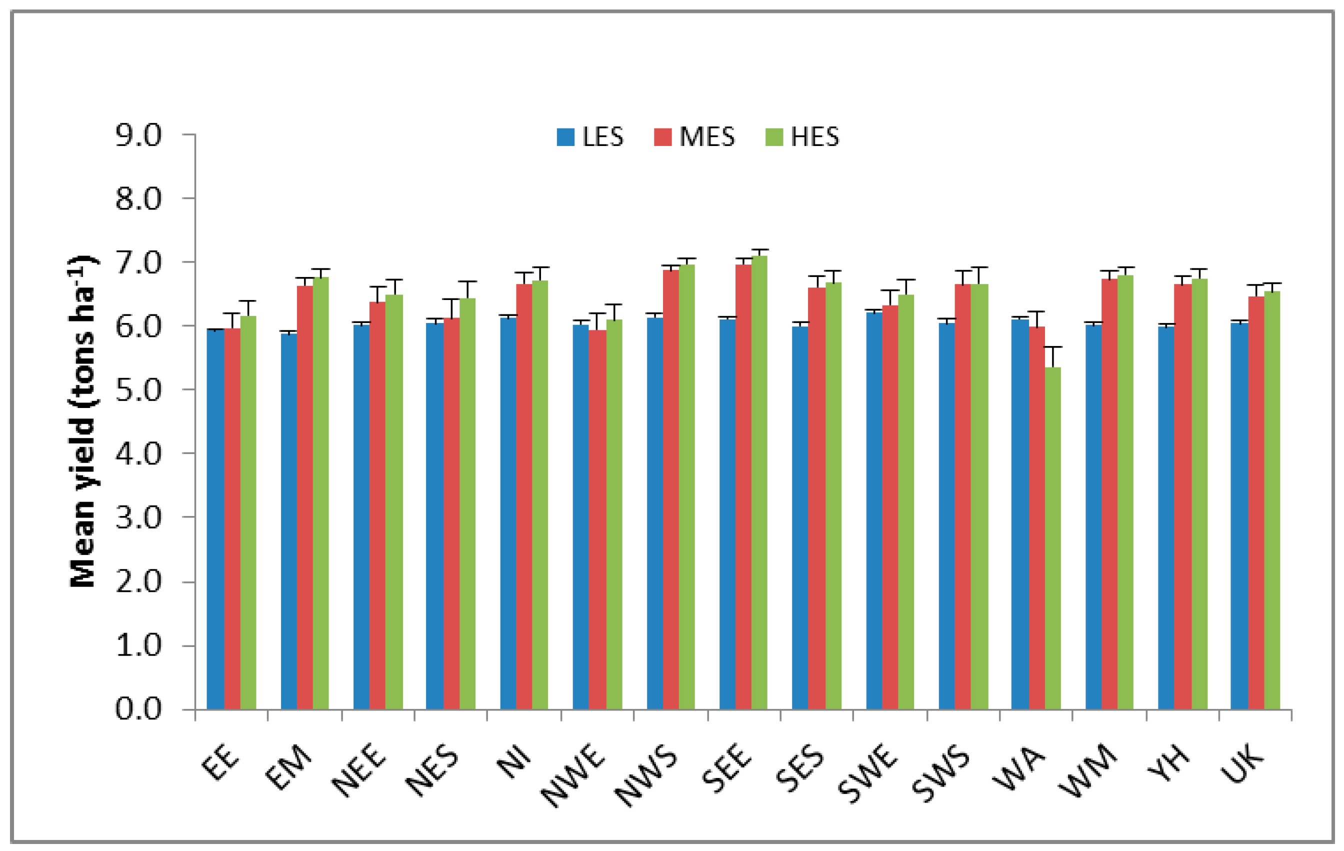
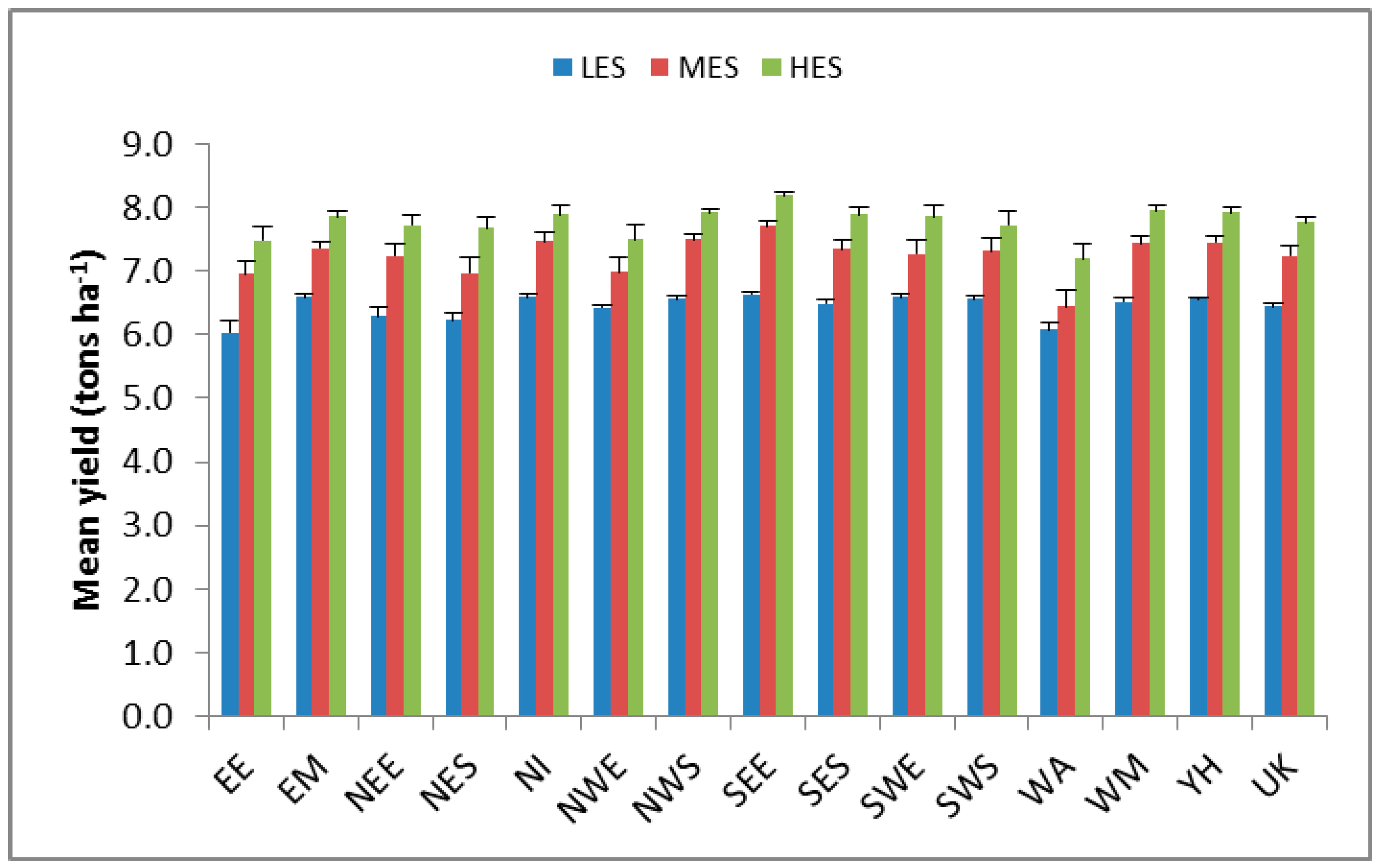
3.3. Simulated Future Yields of Barley

In the 2030s, simulated mean yields of barley for the LES ranged from 5.87 (EM) to 6.20 tons·ha⁻¹ (SWE) with a UK average of 6.04 tons·ha⁻¹ (Figure 4). Only Eastern England, East Midlands (EM) and Yorkshire and Humber (YH) had mean yields under 6.0 tons·ha⁻¹. The 90th and 10th percentile yield values ranged from 6.16 to 6.57 tons·ha⁻¹ and 5.61 to 5.93 tons·ha⁻¹ respectively (

Table 4. Descriptive statistics of simulated barley yields in the 2030s under the LES, MES and HES.

	EE	EM	NEE	NES	NI	NWE	NWS	SEE	SES	SWE	SWS	WA	WM	YH	UK
Statistic	LES
Mean	5.92	5.87	6.01	6.04	6.12	6.03	6.13	6.11	6.00	6.20	6.05	6.11	6.01	5.99	6.04
Std. Error	0.04	0.04	0.06	0.06	0.06	0.06	0.06	0.05	0.07	0.04	0.07	0.04	0.04	0.05	0.05
Std. Dev.	0.21	0.23	0.31	0.33	0.32	0.32	0.32	0.25	0.36	0.23	0.37	0.24	0.23	0.26	0.27
Median	5.91	5.88	5.96	6.00	6.04	6.01	6.16	6.07	6.00	6.16	6.05	6.07	5.98	5.96	6.01
90th	6.16	6.16	6.49	6.54	6.57	6.48	6.54	6.45	6.52	6.49	6.57	6.50	6.32	6.35	6.45
10th	5.76	5.68	5.66	5.70	5.74	5.67	5.76	5.80	5.61	5.93	5.65	5.86	5.77	5.69	5.71
Skewness	−0.83	−1.15	0.09	−0.03	0.26	0.31	−0.12	0.23	0.06	0.23	0.12	0.51	−0.03	0.19	0.22
Min.	5.25	5.08	5.44	5.37	5.60	5.58	5.43	5.74	5.30	5.80	5.41	5.68	5.49	5.50	5.60
Max.	6.32	6.23	6.57	6.62	6.73	6.67	6.75	6.61	6.65	6.71	6.71	6.65	6.44	6.51	6.56
	MES
Mean	5.96	6.64	6.38	6.13	6.66	5.94	6.88	6.96	6.61	6.33	6.65	5.99	6.73	6.65	6.46
Std. Error	0.24	0.12	0.24	0.29	0.17	0.26	0.07	0.10	0.18	0.23	0.23	0.25	0.13	0.13	0.19
Std. Dev.	1.33	0.68	1.29	1.61	0.94	1.42	0.41	0.57	0.97	1.29	1.23	1.37	0.70	0.74	1.04
Median	6.34	6.75	6.74	6.75	6.90	6.55	6.88	6.96	6.88	6.76	6.92	6.50	6.81	6.64	6.74
90th	7.21	7.33	7.44	7.48	7.49	7.15	7.36	7.59	7.45	7.35	7.54	7.28	7.42	7.40	7.39
10th	4.30	5.88	4.73	3.01	5.37	4.01	6.40	6.40	4.89	4.79	6.32	4.02	5.97	5.98	5.15
Skewness	−1.38	−1.71	−1.63	−1.32	−1.55	−1.37	−0.35	−0.89	−1.41	−2.17	−2.78	−1.33	−1.44	−1.41	−1.48
Min	1.93	4.16	2.66	2.58	3.79	1.86	5.90	5.46	4.33	1.54	2.29	2.05	4.39	4.24	3.37
Max	7.46	7.52	7.69	7.59	7.71	7.59	7.60	7.78	7.70	7.61	7.77	7.45	7.57	7.60	7.62
	HES
Mean	6.17	6.76	6.50	6.45	6.72	6.09	6.97	7.10	6.68	6.49	6.66	5.36	6.79	6.75	6.53
Std Error	0.23	0.12	0.23	0.25	0.19	0.26	0.09	0.11	0.19	0.23	0.25	0.30	0.13	0.15	0.13
Std. Dev.	1.28	0.66	1.29	1.37	1.04	1.41	0.49	0.59	1.02	1.24	1.38	1.65	0.72	0.84	0.71
Median	6.50	6.78	6.70	6.74	6.89	6.59	6.98	6.99	6.82	6.79	6.91	5.94	6.84	6.75	6.58
90th Perc.	7.35	7.48	7.62	7.72	7.74	7.49	7.56	7.83	7.70	7.64	7.72	6.90	7.63	7.68	7.41
10th	4.36	6.06	4.93	3.78	5.22	4.29	6.40	6.61	5.03	5.14	6.14	2.81	6.08	5.89	5.79
Skewness	−1.41	−1.11	−1.51	−1.28	−1.38	−1.35	0.01	−0.24	−1.19	−2.11	−2.52	−0.87	−1.41	−1.11	−0.77
Minimum	2.19	4.56	2.72	3.44	3.66	2.00	6.08	5.80	4.25	1.84	1.93	1.55	4.28	4.15	4.55
Maximum	7.68	7.76	7.91	7.94	7.96	7.79	7.93	8.07	7.92	7.96	8.01	7.62	7.76	7.91	7.56

Note: 90th and 10th are percentiles.

). For the UK, the 90th and 10th percentiles were 6.45 and 5.71 tons·ha⁻¹ respectively.

Under the MES, the mean yields ranged from 5.94 (NWE) to 6.96 tons·ha⁻¹ (SEE), and 6.46 tons·ha⁻¹ for the UK (Figure 4). The 90th and 10th percentiles of yields ranged from 7.15 to 7.59 tons·ha⁻¹ and 3.01 to 6.40 tons·ha⁻¹ respectively (Table 2). For the UK, the 90th and 10th percentiles were 7.39 and 6.74 tons·ha⁻¹ respectively. Mean yields, under the HES, ranged from 5.36 (WA) to 7.10 tons·ha⁻¹ (SEE), with 6.53 tons·ha⁻¹ for the UK. Only SEE had a mean yield over 7 tons·ha⁻¹. The 90th and 10th percentile yield values ranged from 6.90 to 7.83 tons·ha⁻¹ and 2.81 to 6.61 tons·ha⁻¹, respectively. As indicated by the standard error and deviation values, there was little variability in yields within model variants and across the regions.

In the 2040s, simulated mean yield values under the LES for all regions ranged from 6.08 (EM) to 6.41 tons·ha⁻¹ (SWE), with 6.24 tons·ha⁻¹ for the UK (Figure 5,

Table 5. Descriptive statistics of simulated barley yields (tons·ha⁻¹) in the 2040s under the LES, MES and HES.

	EE	EM	NEE	NES	NI	NWE	NWS	SEE	SES	SWE	SWS	WA	WM	YH	UK
Statistic	LES
Mean	6.12	6.08	6.21	6.24	6.32	6.24	6.35	6.35	6.19	6.41	6.21	6.31	6.20	6.19	6.24
Std. Error	0.04	0.04	0.06	0.06	0.06	0.05	0.06	0.04	0.07	0.04	0.06	0.04	0.04	0.04	0.04
St. Dev.	0.20	0.21	0.31	0.31	0.31	0.29	0.31	0.21	0.36	0.21	0.35	0.22	0.19	0.25	0.25
Median	6.11	6.08	6.21	6.23	6.30	6.23	6.34	6.33	6.13	6.38	6.19	6.28	6.23	6.18	6.21
90th	6.35	6.28	6.66	6.70	6.74	6.61	6.74	6.60	6.70	6.65	6.70	6.60	6.44	6.51	6.58
10th	5.91	5.89	5.84	5.86	5.94	5.87	5.97	6.09	5.77	6.17	5.80	6.08	5.96	5.88	5.92
Skewness	−1.12	−1.25	0.09	−0.09	0.18	0.17	−0.17	0.10	0.04	0.17	0.16	0.02	−0.31	0.03	0.13
Minimum	5.45	5.34	5.67	5.64	5.83	5.83	5.69	5.97	5.54	6.04	5.64	5.82	5.73	5.74	5.83
Maximum	6.43	6.45	6.75	6.78	6.87	6.76	6.91	6.74	6.80	6.84	6.82	6.72	6.52	6.64	6.69
	MES
Mean	6.49	7.10	6.72	6.45	7.07	6.44	7.21	6.24	6.90	6.65	6.95	5.38	7.19	7.05	6.70
SE	0.23	0.09	0.23	0.29	0.15	0.25	0.07	0.25	0.19	0.25	0.24	0.32	0.09	0.12	0.20
SD	1.25	0.47	1.24	1.60	0.81	1.36	0.38	1.38	1.03	1.38	1.30	1.73	0.48	0.65	1.08
Median	6.89	7.13	7.12	7.09	7.24	7.08	7.24	6.76	7.23	7.15	7.22	5.69	7.17	7.09	7.01
90th	7.55	7.69	7.80	7.68	7.79	7.53	7.75	7.64	7.76	7.65	7.88	7.18	7.73	7.81	7.67
10th	4.93	6.48	5.34	3.46	6.02	4.23	6.72	4.07	5.07	5.09	6.59	2.90	6.65	6.02	5.25
Skewness	−1.73	−0.48	−1.62	−1.31	−1.46	−1.66	−0.19	−0.91	−1.34	−2.22	−2.72	−0.86	−0.72	−0.75	−1.28
Min	2.12	5.90	3.14	2.95	4.52	2.24	6.48	2.76	4.57	1.47	2.42	1.49	5.92	5.45	3.67
Max	7.82	7.86	7.97	7.90	8.02	7.76	7.82	8.02	8.00	7.97	8.03	7.77	7.85	7.93	7.91
	HES
Mean	6.94	7.49	7.07	7.09	7.42	6.64	7.45	7.59	7.33	7.12	7.19	5.89	7.33	7.34	7.14
Standard Error	0.23	0.09	0.24	0.24	0.17	0.25	0.09	0.11	0.15	0.21	0.24	0.30	0.11	0.12	0.12
Std. Dev.	1.24	0.50	1.32	1.33	0.91	1.36	0.51	0.62	0.80	1.14	1.30	1.64	0.60	0.68	0.64
Median	7.25	7.57	7.35	7.45	7.54	7.06	7.48	7.44	7.31	7.37	7.36	6.47	7.21	7.29	7.13
90th	7.99	8.10	8.17	8.23	8.25	7.88	8.11	8.34	8.20	8.02	8.26	7.45	8.09	8.18	7.88
10th	5.39	6.89	5.70	4.56	6.25	4.50	6.81	7.09	6.43	5.76	6.65	3.48	6.74	6.49	6.44
Skewness	−1.88	−0.44	−1.54	−1.25	−1.31	−1.53	−0.04	−0.32	−0.86	−2.13	−2.46	−1.03	−0.18	−0.21	−0.70
Minimum	2.41	6.25	3.31	4.23	4.68	2.37	6.59	6.13	5.43	2.80	2.66	1.94	5.83	5.95	5.30
Maximum	8.30	8.29	8.43	8.44	8.47	8.12	8.32	8.58	8.44	8.51	8.53	8.16	8.22	8.37	8.11

Note: 90th and 10th are percentiles.

). The 90th and 10th percentile yield values ranged from 6.28 to 6.74 tons·ha⁻¹ and 5.77 to 6.17 tons·ha⁻¹ respectively. Yields for Eastern England, East Midlands, North East Scotland, North West Scotland (NWS) and West Midlands (WM) were negatively skewed. Under the MES, simulated mean yields ranged from 5.38 (WA) to 7.21 tons·ha⁻¹ (NWS) and 6.70 tons·ha⁻¹ for the UK. Five regions (EM, NI, NWS, WM and YH) had mean yields just over 7.0 tons·ha⁻¹. The 90th and 10th percentiles ranged from 7.53 to 7.88 tons·ha⁻¹ and 2.90 to 6.70 tons·ha⁻¹ respectively. Under the HES, regional mean yields ranged from 5.89 (WA) to 7.59 tons·ha⁻¹ (SEE), with an average of 7.14 tons·ha⁻¹ for the UK. Only EE, NWE and WA had mean yields lower than 7 tons·ha⁻¹. The 90th and 10th percentiles ranged from 7.45 to 8.34 tons·ha⁻¹ and 3.48 to 7.09 tons·ha⁻¹ respectively. All the regional yield values under both MES and HES were negatively skewed.

In the 2050s, mean yields for all UK regions increase over previous time slices for all emissions scenarios. Mean regional yields under the LES ranged from 6.03 (EE) to 6.63 tons·ha⁻¹ (SEE), with 6.44 tons·ha⁻¹ for the UK (Figure 6,

Table 6. Descriptive statistics of simulated barley yields in the 2050s under the LES, MES and HES.

	EE	EM	NEE	NES	NI	NWE	NWS	SEE	SES	SWE	SWS	WA	WM	YH	UK
	LES
Mean	6.03	6.59	6.29	6.23	6.59	6.42	6.57	6.63	6.48	6.60	6.56	6.08	6.52	6.55	6.44
Std. Error	0.18	0.04	0.13	0.12	0.06	0.05	0.04	0.04	0.06	0.04	0.04	0.11	0.06	0.04	0.05
Std. Dev.	0.97	0.21	0.69	0.67	0.31	0.30	0.20	0.20	0.34	0.22	0.22	0.60	0.32	0.22	0.26
Median	6.34	6.58	6.50	6.44	6.66	6.43	6.59	6.64	6.54	6.59	6.58	6.24	6.57	6.55	6.46
90th	6.62	6.81	6.71	6.62	6.81	6.77	6.80	6.86	6.76	6.86	6.82	6.73	6.82	6.82	6.75
10th	4.47	6.44	6.08	5.96	6.38	6.21	6.30	6.40	6.16	6.43	6.27	5.38	6.10	6.31	6.10
Skewness	−2.13	−1.43	−3.75	−2.95	−3.31	−1.51	−0.38	−1.14	−2.55	−1.43	−0.54	−0.94	−2.17	−1.35	−0.77
Minimum	2.84	5.89	3.12	3.61	5.21	5.37	6.07	5.99	5.11	5.88	6.03	4.57	5.28	5.79	5.81
Maximum	6.82	6.86	6.80	6.76	6.90	6.82	6.89	6.89	6.84	6.88	6.90	6.78	6.86	6.85	6.82
	MES
Mean	6.95	7.36	7.23	6.97	7.47	6.98	7.49	7.70	7.34	7.27	7.32	6.44	7.44	7.45	7.24
Std. Error	0.21	0.09	0.19	0.26	0.13	0.23	0.08	0.08	0.15	0.21	0.22	0.28	0.11	0.10	0.17
Std. Dev.	1.15	0.50	1.02	1.41	0.72	1.24	0.41	0.44	0.83	1.14	1.18	1.51	0.60	0.57	0.91
Median	7.19	7.45	7.50	7.51	7.64	7.45	7.50	7.71	7.59	7.59	7.60	7.11	7.52	7.52	7.49
90th	7.80	7.92	8.00	8.07	8.12	8.01	7.97	8.19	8.10	8.08	8.13	7.68	8.03	8.00	8.01
10th	5.61	6.92	6.26	4.05	6.68	5.69	6.98	7.28	6.12	5.93	7.08	4.30	6.93	6.95	6.20
Skewness	−2.27	−1.98	−2.09	−1.48	−1.90	−1.99	−0.88	−0.82	−1.50	−2.76	−2.98	−1.33	−1.98	−1.73	−1.83
Minimum	2.57	5.40	3.87	3.85	4.98	2.66	6.22	6.50	5.23	2.57	2.94	2.15	5.15	5.42	4.25
Maximum	8.11	8.11	8.20	8.19	8.25	8.20	8.12	8.32	8.26	8.32	8.22	8.04	8.11	8.11	8.18
	HES
Mean	7.49	7.85	7.72	7.67	7.89	7.50	7.93	8.18	7.89	7.85	7.72	7.19	7.96	7.91	7.77
Std. Error	0.20	0.08	0.17	0.17	0.13	0.22	0.06	0.07	0.12	0.17	0.22	0.24	0.09	0.10	0.09
Std. Dev.	1.11	0.43	0.94	0.95	0.74	1.19	0.33	0.39	0.63	0.92	1.20	1.31	0.47	0.53	0.49
Median	7.79	7.92	7.99	7.96	8.07	7.93	7.94	8.19	8.04	8.11	7.99	7.75	8.01	8.00	7.87
90th	8.25	8.35	8.41	8.49	8.53	8.38	8.37	8.60	8.49	8.51	8.57	8.24	8.38	8.44	8.27
10th	6.38	7.40	7.02	6.03	7.01	6.50	7.44	7.84	7.06	7.09	7.42	5.55	7.52	7.48	7.33
Skewness	−2.60	−1.61	−2.42	−1.51	−2.00	−2.47	−0.38	−1.22	−1.34	−3.06	−2.91	−1.69	−2.15	−1.96	−1.53
Minimum	3.02	6.30	4.43	5.33	5.24	2.92	7.26	6.95	6.16	3.88	3.32	3.08	6.10	5.93	6.09
Maximum	8.53	8.50	8.54	8.62	8.68	8.59	8.43	8.73	8.67	8.71	8.70	8.48	8.51	8.47	8.37

Note: 90th and 10th are percentiles.

). The 90th and 10th percentiles ranged from 6.62 to 6.86 tons·ha⁻¹ and 4.47 to 6.44 tons·ha⁻¹, respectively. Mean regional yields under the MES ranged 6.44 (WA) to 7.70 tons·ha⁻¹ (SEE), with a UK average of 7.24 tons·ha⁻¹. The 90th and 10th percentiles ranged from 7.68 to 8.19 tons·ha⁻¹ and 4.05 to 7.28 tons·ha⁻¹ respectively. Only four regions (EE, EM, NWS and WA) had 90th percentile yield values lower than 8 tons·ha⁻¹. Simulated mean regional yields under the HES ranged from 7.49 (EE) to 8.18 tons·ha⁻¹ (SEE). The average yield for the UK was 7.77 tons·ha⁻¹. The 90th and 10th percentiles for the regional yields ranged from 8.24 to 8.60 tons·ha⁻¹ and 5.55 to 7.84 tons·ha⁻¹, respectively. The 90th and 10th percentiles for the UK were 8.27 and 7.33 tons·ha⁻¹ respectively. The yield values were negatively skewed for all regions and emissions scenarios.

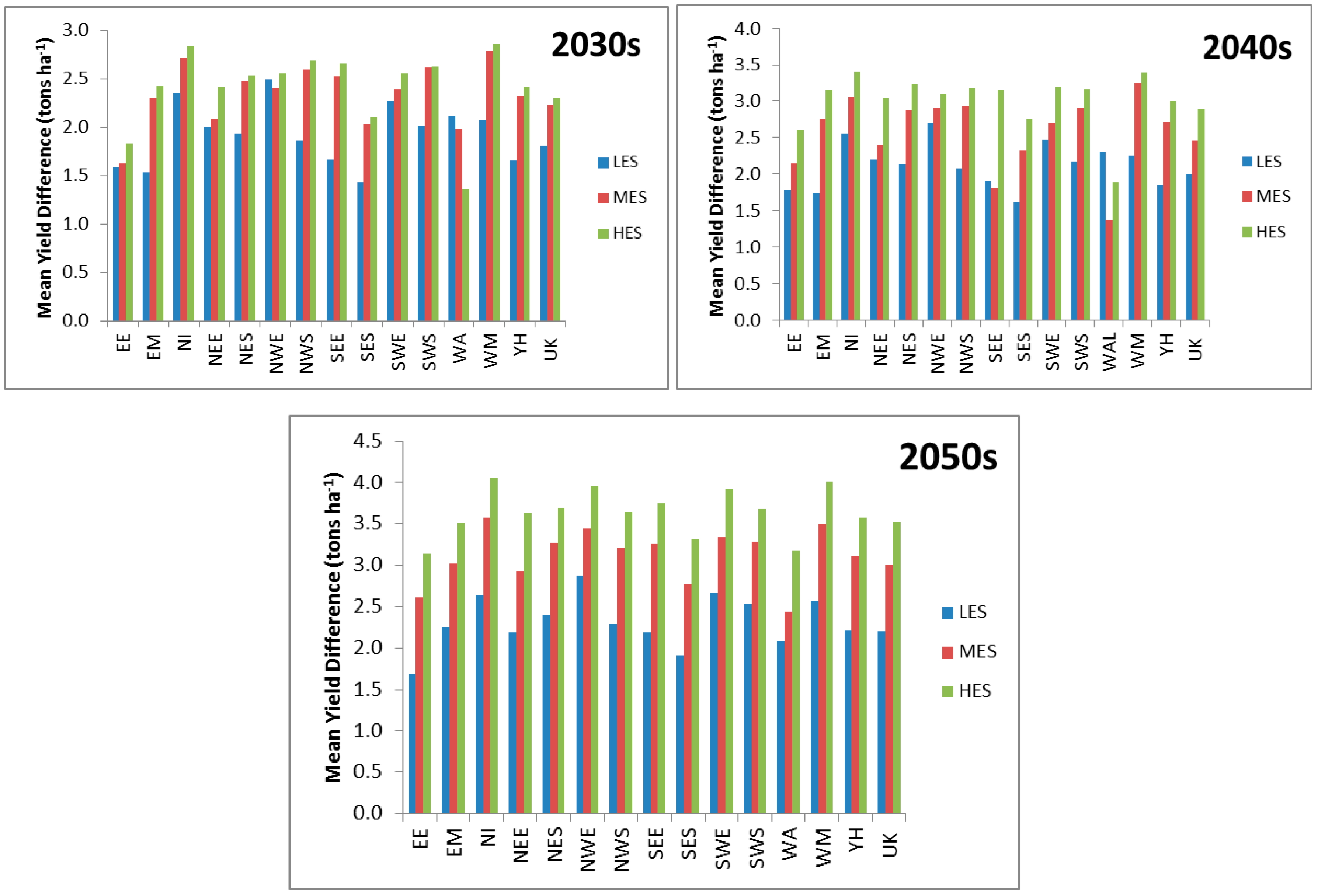
3.4. Differences between Future and Baseline Yields

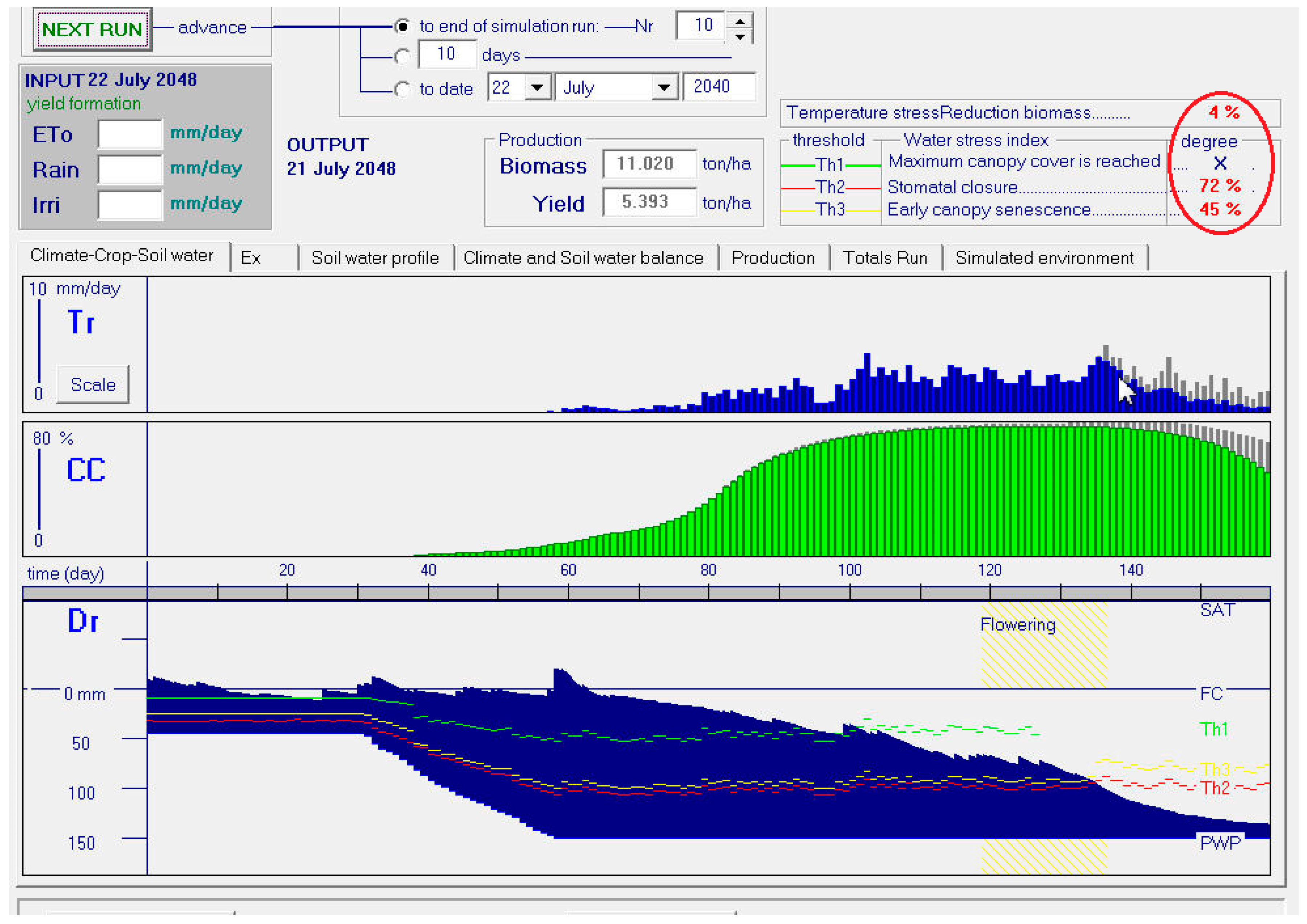
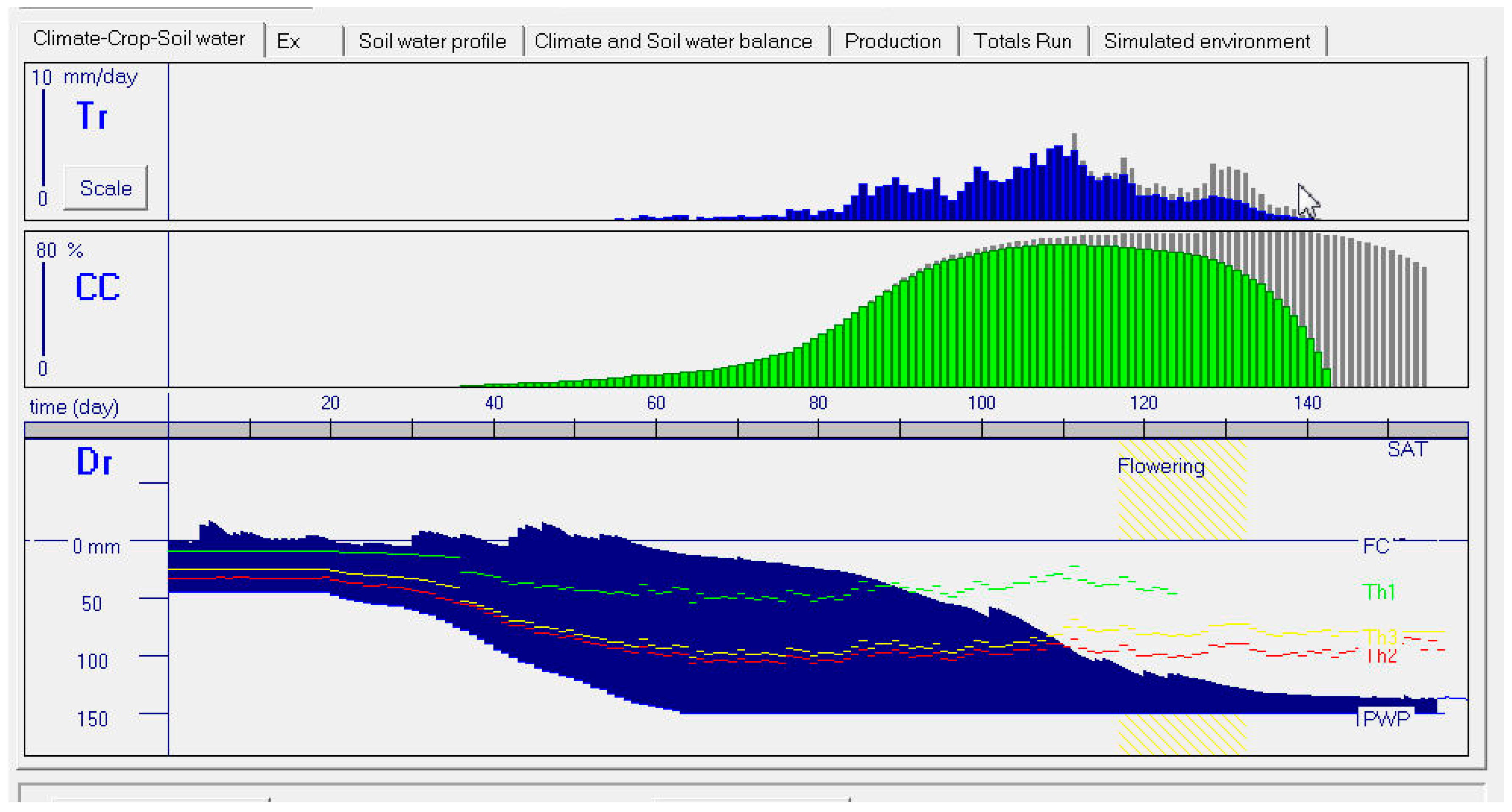
Relative to the yields in the baseline period (1960–1990), simulated barley yields increased over baseline yields for all time slices, emissions scenarios and regions, with the exception of NWE in the 2030s and WA in the 2030s and 2040s (Figure 7). Similarly, the simulated future yields were greater than the 2010 regional yields for England and the UK average yield (Figure 3) for all time slices and emissions scenarios. The pattern and magnitude of differences represent the general trend in yields in the future time slices and emissions scenarios presented earlier. Thus, the greatest increases in yields were observed under the HES in the 2050s. Changes in mean yields for all regions, emissions scenarios and time slices ranged from 1.43 to 4.05 tons·ha⁻¹. Except for WA in the 2030s and 2040s, absolute increases in projected yields over the baseline yields for all time slices and emissions scenarios were generally higher in the western than the eastern regions of the UK, but marginally from south to north. For each emission scenario, however, changes in yields between time slices were not substantial under the LES but were greater under the MES and HES. The difference between the MES and HES was not substantial and less obvious in the 2030s compared to the 2040s and 2050s.

3.5. Dips in Yields

Temporal trends in the simulated future yields showed some dips within time slices for all emission scenarios (Supplementary Materials Figures S1–S9). The frequency and depth of the dips in yields increased from the 2030s to the 2050s and from LES to HES. These dips always resulted from a subset of the climatic variants of a given emissions scenario. For example, yields under 2 tons·ha⁻¹ were observed for some regions in some climate variants in the 2040s and 2050s under the HES. Stresses related to temperature and water could principally account for the yield dips even though it was not always clear. In AquaCrop, these stresses result in reduction in biomass production and HIo. This is exemplified by Figure 8 and Figure 9 (representing selected climatic variants under the HES). Figure 8 represents a situation in which water stress resulted in stomatal closure, early canopy senescence and biomass reduction. Figure 9 represents a situation where water stresses coincided with either anthesis or post-anthesis, resulting in large reductions in both biomass production and yield. Soil water content exceeding the anaerobiosis point was also observed, sometimes around anthesis, for some climatic variants.

4. Discussion

4.1. Sowing Date as a Source of Uncertainty

Tracking and quantifying the aggregate effect of all uncertainties on simulated yields in climate change studies are difficult and require complex mathematical procedures [44]. The uncertainties can arise from the projected climate change data (due to, for example, uncertainties in the emissions scenarios), the crop growth simulation model, and the soil and crop input data, including sowing dates [37,44,45]. Sowing date affects crop phenology and therefore biomass production, abiotic stresses and yields [3,29,46,47]. Sowing dates are highly variable over time and space [14,46]. Using actual sowing date can help minimize uncertainties but it is difficult to accurately predict future sowing dates under climate change. Hence, climate change studies rely on current sowing dates and adjustments are explored as part of adaptation planning for future climates [3,14,48,49]. Indicative sowing dates become useful when data on actual sowing dates are lacking. The low RMSE values observed in the current study suggest that the sowing dates used are acceptable.

4.2. Yields under Climate Change

The baseline yields show an increasing trend, with 90th percentile of yields around 5 tons·ha⁻¹. This could be due to a combination of genetic improvement, favourable environmental conditions and improved management practices. Regional mean yields for barley for the period 2000–2010 ranged from 4.6 to 5.5 tons·ha⁻¹. In 2010, mean spring barley yield for the UK was 5.2 tons·ha⁻¹, with a mean yield of 4.9 tons·ha⁻¹ for England and 5.4 tons·ha⁻¹ for the rest of the UK (Figure 3). McKenzie et al. [50] have reported yields as high as 6–10 tons·ha⁻¹ from field experiments with the genotype Westminster in southeast Scotland.

The simulation results show that projected climate change can be beneficial to grain yield of barley across the UK. Barley yields for all UK regions increased over baseline yields for all emission scenarios and time slices. Yield increases were greater under the HES, followed by the MES and in the 2050s compared to the earlier time slices. For example, the 90th percentile of yields in the 2050s, under the HES, exceeds 8 tons·ha⁻¹, with greatest absolute increase in yields occurring in southeast England. Geographically, the greatest increases in yields relative to the baseline occur in the western half of the UK (except Wales in some instances) even though the east-west yield gradient observed in the baseline period will remain unchanged. The low values of standard deviation and skewness in the simulated yields suggest high certainty in yields [5]. The low variability in regional yields is consistent with the observed variability in the baseline yields. However, the low variability in yields observed across emission scenarios might be due to the small differences in climatic conditions (including atmospheric CO₂) up to the 2050s. Differences in climatic variables for the different emission scenarios become substantial after the 2050s [33,49]. However, for the MES and HES, the 10th percentile values had a wider range and the difference between the lowest 90th and 10th percentile values were also large for all time slices. For Wales, mean yields were higher under the LES than the other emission scenarios in the 2030s and 2040s (Figure 5 and Figure 6). It was not clear which environmental conditions produced the deviation from the observed pattern across the emissions scenarios. However, this might be due to uncertainties associated with the sowing date or the climatic variants. Wales recorded the highest RMSE related to the accuracy of sowing dates (Table 3). There was less variability in yields for Wales under the LES than for the other emissions scenarios in the 2030s and 2040s, evidenced by the increasing standard deviations and skewness (Table 4 and Table 5).

There are very few simulation studies for barley crops under current conditions in northern temperate environments and fewer under future climates [3,29]. The observed increases in yields over the baseline yields are consistent with previous studies. Using weather generator data from the UKCP09, Rivington and colleagues [51] reported that the mode of simulated barley grain yields in Scotland exceeded 7 tons·ha⁻¹ in the 2040s under the HES. In Ireland, barley grain yields can exceed 8 tons·ha⁻¹ in 2055 even though current spatial distribution of yield potential will not change [14]. Similarly, Richter et al. [5] reported that wheat yields in England and Wales are likely to increase by up to 2 tons·ha⁻¹ over baseline yields despite projected reductions in summer rains. The greatest increases were found to occur in East Anglia and the south east. These studies attributed the potential increase in yields to elevated atmospheric CO₂ concentration. Studies in other temperate European environments also reported increases in barley biomass and grain yields under elevated atmospheric CO₂ concentrations [8,12,16].

The observed variations in yields between time slices in the current study might be due to elevated atmospheric CO₂ in combination with small increases in temperature and changes in rainfall to proportionately increase biomass and grain yield so that grain:biomass ratio remains unchanged [14]. This favourable effect of climate change might also account for the greater absolute increase in yield over baseline yields in the western half of the UK where wet conditions around anthesis might be suppressing yields under current conditions [9]. Generally, C₃ crops in northern temperate environments are expected to benefit substantially from elevated atmospheric CO₂ concentration and moderate warming when water is not limiting [3,4,5,6]. This positive effect has been found to arise mainly from greater biomass production and grain number [8,12,15,16] and, to a lesser extent, from increased grain weight due to interactions between CO₂, temperature and water on the duration and effectiveness of grain filling and canopy senescence [15].

4.3. Stresses and Risks to Yields

Even though the results of the current study suggest yield stability and viability of UK barley production in the future, other stresses related to heat and soil water dynamics might cause yield penalties in some years [3,6,20,52] as indicated by the occasional yield dips (Supplementary Materials Figures S3–S9). In AquaCrop, thresholds for the effects of water and temperature stresses on biomass production are executed mainly through changes in canopy expansion, stomatal closure and early senescence [31]. Water stress (under both deficit and saturated conditions) and temperature stresses affect yield directly through pollination failure and reductions in reference harvest index (Figure 8 and Figure 9). The situations exemplified by Figure 8 and Figure 9 can result in reductions in biomass production and yield by suppressing transpiration. While the excessive soil water content affected almost all the regions, it was prevalent in Wales, South West Scotland and Northern Ireland where the initial canopy development was adversely affected and maximum canopy cover was not reached.

Reductions in biomass production due to temperature stress in some climatic variants ranged from 2% to 53% across emission scenarios and time slices, with the largest reductions occurring under the HES in Eastern England. This suggests that even though barley is known to be drought tolerant, heat stress can limit productivity in some UK regions under projected climates, especially under the HES. It has been reported that heat stress, due to climate change, is an important source of threat to wheat yields in England and Wales [5] and in Europe [18] or barley production in Finland and Denmark [3,8]. The risk is that the years in the time slices in the current study do not represent actual future years, implying that the observed stresses can occur in any crop season in the future under the projected climate change conditions. Hence, there is the need to adapt crops or management practices in response to such stressful conditions even though early maturity, due to faster accumulation of total thermal time, might enable the crops avoid heat or water deficit stresses in the summer.

5. Conclusions

Barley is likely to remain a viable rain-fed crop in the UK under the projected climate change from the 2030s to the 2050s. For all time slices and emission scenarios, mean yields for all UK regions increased over the baseline yields, with greatest increases occurring in the 2050s. The increase in yields for the emissions scenarios followed the order: HES > MES > LES. Absolute increases in yields over the baseline yields were greater in the western half than the eastern regions of the UK. However, stresses related to heat, soil water deficits and surplus pose risks to stable and high yields as they can cause substantial yield penalties in some years. Adaptation planning in response to these potential risks is recommended. The effects of extreme events and their intensities, or the probability of exceeding a certain threshold of climate change signal (e.g., increase in temperature exceeding 4 °C) were not assessed. These are crucial for quantifying and better understanding risks and planning adaptation especially when heat stress has been found to be a potential threat.

References

1. Newton, A.C.; Flavell, A.J.; George, T.S.; Leat, P.; Mulholland, B.; Ramsay, L.; Revoredo-Giha, C.; Russell, J.; Steffenson, B.J.; Swanston, J.S.; et al. Crops that feed the world 4. Barley: A resilient crop? Strengths and weaknesses in the context of food security. Food Secur. 2011, 3, 141–178. [Google Scholar] [CrossRef]
2. Department of Environment, Food and Rural Affairs (Defra). Agriculture in the United Kingdom 2011; Produced for National Statistics; Department of Environment, Food and Rural Affairs (Defra): York, UK, 2011.
3. Rötter, R.P.; Palosuo, T.; Pirttioja, N.K.; Dubrovsky, M.; Salo, T.; Fronzek, S.; Aikasalo, R.; Trnka, M.; Ristolainen, A.; Carter, T.R. What would happen to barley production in Finland if global warming exceeded 4 °C? A model-based assessment. Eur. J. Agron. 2011, 35, 205–214. [Google Scholar] [CrossRef]
4. DaMatta, F.M.; Grandis, A.; Arenque, B.C.; Buckeridge, M.S. Impacts of climate change on crop physiology and food quality. Food Res. Int. 2010, 43, 1814–1823. [Google Scholar] [CrossRef]
5. Richter, G.M.; Semenov, M.A. Modelling impacts of climate change on wheat yields in England and Wales: Assessing drought risks. Agric. Syst. 2005, 84, 77–97. [Google Scholar] [CrossRef]
6. Fuhrer, J. Agroecosystem responses to combinations of elevated CO2, ozone and global climate change. Agric. Ecosyst. Environ. 2003, 97, 1–20. [Google Scholar] [CrossRef]
7. Claesson, J.; Nycander, J. Combined effects of global warming and increased CO2-concentration on vegetation growth in water-limited conditions. Ecol. Model. 2013, 256, 23–30. [Google Scholar] [CrossRef]
8. Clausen, S.K.; Frenck, G.; Linden, L.G.; Mikkelsen, T.N.; Lunde, C.; Jørgensen, R.B. Effects of single and multifactor treatments with elevated temperature, CO2 and ozone on oilseed rape and barley. J. Agron. Crop Sci. 2011, 197, 442–453. [Google Scholar] [CrossRef]
9. Robredo, A.; Pérez-López, U.; Miranda-Apodaca, J.; Lacuesta, M.; Mena-Petite, A.; Muñoz Rueda, A. Elevated CO2 reduces the drought effect on nitrogen metabolism in barley plants during drought and subsequent recovery. Environ. Exp. Bot. 2011, 71, 399–408. [Google Scholar] [CrossRef]
10. Robredo, A.; Pérez-López, U.; de la Maza, H.S.; González-Moro, B.; Lacuesta, M.; Mena-Petite, A.; Muñoz-Rueda, A. Elevated CO2 alleviates the impact of drought on barley improving water status by lowering stomatal conductance and delaying its effects on photosynthesis. Environ. Exp. Bot. 2007, 59, 252–263. [Google Scholar] [CrossRef]
11. Wall, G.W.; Garcia, R.L.; Wechsung, F.; Kimball, B.A. Elevated atmospheric CO2 and drought effects on leaf gas exchange properties of barley. Agric. Ecosyst. Environ. 2011, 144, 390–404. [Google Scholar] [CrossRef]
12. Manderscheid, R.; Pacholski, A.; Frühauf, C.; Weigel, H.-J. Effects of free air carbon dioxide enrichment and nitrogen supply on growth and yield of winter barley cultivated in a crop rotation. Field Crops Res. 2009, 119, 185–196. [Google Scholar] [CrossRef]
13. Barnabás, B.; Jäger, K.; Fehér, A. The effect of drought and heat stress on reproductive processes in cereals. Plant Cell Environ. 2008, 31, 11–38. [Google Scholar] [CrossRef] [PubMed]
14. Holden, N.M.; Brereton, A.J.; Fealy, R.; Sweeney, J. Possible change in Irish climate and its impact on barley and potato yields. Agric. For. Meteorol. 2003, 116, 181–196. [Google Scholar] [CrossRef]
15. Fangmeier, A.; Chrost, B.; Högy, P.; Krupinska, K. CO2 enrichment enhances flag leaf senescence in barley due to greater grain nitrogen sink capacity. Environ. Exp. Bot. 2000, 44, 151–164. [Google Scholar] [CrossRef]
16. Sæbø, A.; Mortensen, L.M. Growth, morphology and yield of wheat, barley and oats grown at elevated atmospheric CO2 concentration in a cool maritime climate. Agric. Ecosyst. Environ. 1996, 57, 9–15. [Google Scholar] [CrossRef]
17. Anjum, S.A.; Xie, X.; Wang, L.C.; Saleem, M.F. Morphological, physiological and biochemical responses of plants to drought stress. Afr. J. Agric. Res. 2011, 6, 2026–2032. [Google Scholar]
18. Semenov, M.A.; Shewry, P.R. Modelling predicts that heat stress, not drought, will increase vulnerability of wheat in Europe. Sci. Rep. 2011, 1, 1–5. [Google Scholar] [CrossRef] [PubMed]
19. González, A.; Martin, I.; Ayerbe, L. Barley yield in water-stress conditions: The influence of precocity, osmotic adjustment and stomatal conductance. Field Crops Res. 1999, 62, 23–34. [Google Scholar] [CrossRef]
20. Ainsworth, E.A.; Rogers, A. The response of photosynthesis and stomatal conductance to rising [CO2]: Mechanisms and environmental interactions. Plant Cell Environ. 2007, 30, 258–270. [Google Scholar] [CrossRef] [PubMed]
21. Steduto, P. Biomass Water-Productivity: Comparing the Growth-Engines of Crop Models; FAO Expert Consultation on Crop Water Productivity under Deficient Water Supply; Food and Agriculture Organization of the United Nations: Rome, Italy, 2003. [Google Scholar]
22. Kuchar, L.; Lipiec, J.; Rejman, J.; Kolodziej, J.; Kaszewski, B. Simulation of potential yields of spring barley in central-eastern Poland using the CERES-Barley model. Acta Agrophys. 2004, 106, 541–551. [Google Scholar]
23. Trnka, M.; Dubrovsky, M.; Žalud, Z. Climate change impacts and adaptation strategies in spring barley production in the Czech Republic. Clim. Chang. 2004, 64, 227–255. [Google Scholar] [CrossRef]
24. Havlinka, P.; Trnka, M.; Eitzinger, J.; Smutný, V.; Thaler, S.; Žalud, Z.; Rischbeck, P.; Křen, J. The performance of CERES-Barley and CERES-Wheat under various soil conditions and tillage practices in Central Europe. Die Bodenkult. 2010, 61, 5–17. [Google Scholar]
25. Travasso, M.I.; Magrin, G.O. Utility of CERES-Barley under argentine conditions. Field Crops Res. 1998, 57, 329–333. [Google Scholar] [CrossRef]
26. Ouda, S.A.; Khalil, F.A.; Afandi, G.E.; Ewis, M.M. Using CropSyst model to predict barley yield under climate change conditions in Egypt: I. Model calibration and validation under current climate. Afr. J. Plant Sci. Biotechnol. 2010, 4, 1–5. [Google Scholar]
27. Ouda, S.A.; Khalil, F.A.; Afandi, G.E.; Ewis, M.M. Using CropSyst model to predict barley yield under climate change conditions in Egypt: II. Simulation of the effect of rescheduling irrigation on barley yield. Afr. J. Plant Sci. Biotechnol. 2010, 4, 6–10. [Google Scholar]
28. Alexandrov, V.; Eitzinger, J.; Cajic, V.; Oberforster, M. Potential impact of climate change on selected agricultural crops in North-Eastern Austria. Glob. Chang. Biol. 2002, 8, 372–389. [Google Scholar] [CrossRef]
29. Rötter, R.P.; Palosuo, T.; Kersebaum, K.C.; Angulo, C.; Bindi, M.; Ewert, F.; Ferrise, R.; Hlavinka, P.; Moriondo, M.; Nende, C.; et al. Simulation of spring barley yield in different climatic zones of Northern and Central Europe: A comparison of nine crop models. Field Crops Res. 2012, 133, 23–36. [Google Scholar] [CrossRef]
30. Todorovic, M.; Albrizio, R.; Zivotic, L.; Saab, A.M.-T.; Stockle, C.; Steduto, P. Assessment of AquaCrop, CropSyst and WOFOST models in the simulation of sunflower growth under different water regimes. Agron. J. 2009, 101, 509–521. [Google Scholar] [CrossRef]
31. Raes, D.; Steduto, P.; Hsiao, T.C.; Fereres, E. AquaCrop—The FAO crop model to simulate yield response to water: II. Main algorithms and software description. Agron. J. 2009, 101, 438–447. [Google Scholar] [CrossRef]
32. Yawson, D.O. Climate Change and Virtual Water: Implications for UK Food Security. Ph.D. Thesis, University of Dundee, Dundee, UK, 2013. [Google Scholar]
33. Murphy, J.M.; Sexton, D.M.H.; Jenkins, G.J.; Boorman, P.; Booth, B.; Brown, K.; Clark, R.; Collin, M.; Harris, G.; Kendon, L.; et al. UK Climate Projections Science Report: Climate Change Projections; Met Office Hadley Centre: Exeter, UK, 2009. [Google Scholar]
34. Jones, P.D.; Kilsby, C.G.; Harpham, C.; Glenis, V.; Burton, A. UK Climate Projections Science Report: Projections of Future Daily Climate for the UK from the Weather Generator; University of Newcastle: Newcastle, UK, 2009. [Google Scholar]
35. Intergovernmental Panel on Climate Change. Climate change 2007: Synthesis report. An assessment of the intergovernmental panel on climate change. In Proceedings of the IPCC Plenary Conference XXVII, Valencia, Spain, 12–17 November 2007.
36. Alexandratos, N.; Bruinsma, J. World Agriculture towards 2030/2050: The 2012 Revision; ESA Working Paper No. 12-03; Food and Agriculture Organization of the United Nations: Rome, Italy, 2012. [Google Scholar]
37. Corfee-Morlot, J.; Höhne, N. Climate change: Long-term targets and short-term commitments. Glob. Environ. Chang. 2003, 13, 277–293. [Google Scholar] [CrossRef]
38. Baruth, B.; Genovese, G.; Montanarella, L. New Soil Information for the MARS Crop Yield Forecasting System; European Commission Directorate General, Joint Research Centre: Ispra, Italy, 2006. [Google Scholar]
39. Steduto, P.; Hsiao, T.C.; Raes, D.; Fereres, E. AquaCrop—The FAO crop model to simulate yield response to water: I. Concepts and underlying principles. Agron. J. 2009, 101, 426–437. [Google Scholar] [CrossRef]
40. Geerts, S.; Raes, D.; Gracia, M.; Miranda, R.; Cusicanqui, J.A.; Taboada, C.; Mendoza, J.; Huanca, R.; Mamani, A.; Condori, O.; et al. Simulating yield response of Quinoa to water availability with AquaCrop. Agron. J. 2009, 101, 499–508. [Google Scholar] [CrossRef]
41. Andarzian, B.; Bannayan, M.; Steduto, P.; Mazraeh, H.; Barati, M.E.; Barati, M.A.; Rahnama, A. Validation and testing of the AquaCrop model under full and deficit irrigated wheat production in Iran. Agric. Water Manag. 2011, 100, 1–8. [Google Scholar] [CrossRef]
42. Mainuddin, M.; Kirby, M.; Hoanh, C.T. Adaptation to climate change for food security in the lower Mekong Basin. Food Secur. 2011, 3, 433–450. [Google Scholar] [CrossRef]
43. Loague, K.; Green, R.E. Statistical and graphical methods for evaluating solute transport models: Overview and application. J. Contam. Hydrol. 1991, 7, 51–73. [Google Scholar] [CrossRef]
44. Yao, F.M.; Qin, P.C.; Zhang, J.H.; Lin, E.; Boken, V. Uncertainties in assessing the effect of climate change on agriculture using model simulation and uncertainty processing methods. Chin. Sci. Bull. 2011, 56, 729–737. [Google Scholar] [CrossRef]
45. Niu, X.; Easterling, W.; Hays, C.; Jacobs, A.; Mearns, L. Reliability and input data induced uncertainty of the EPIC model to estimate climate change impact on sorghum yields in the U.S. Great Plains. Agric. Ecosyst. Environ. 2009, 129, 268–276. [Google Scholar] [CrossRef]
46. Biernath, C.; Gayler, S.; Bittner, S.; Klein, C.; Högy, P.; Fangmeier, A.; Priesack, E. Evaluating the ability of four crop models to predict different environmental impacts on spring wheat grown in open-top chambers. Eur. J. Agron. 2011, 35, 71–82. [Google Scholar] [CrossRef]
47. Guereña, A.; Ruiz-Ramos, M.; Díaz-Ambrona, C.H.; Conde, J.R.; Mínguez, M.I. Assessment of climate change and agriculture in Spain using climate models. Agron. J. 2001, 93, 237–249. [Google Scholar] [CrossRef]
48. Matthews, R.B.; Rivington, M.; Muhammed, S.; Newton, A.C.; Hallet, P.D. Adapting crops and cropping systems to future climates to ensure food security: The role of crop modelling. Glob. Food Secur. 2013, 2, 24–28. [Google Scholar] [CrossRef]
49. Wilby, R.L.; Orr, H.; Watts, G.; Battarbee, R.W.; Berry, P.M.; Chadd, R.; Dugdale, S.J.; Dunbar, M.J.; Elliott, J.A.; Extence, C.; et al. Evidence needed to manage freshwater ecosystems in a changing climate: Turning adaptation principles into practice. Sci. Total Environ. 2010, 408, 4150–4164. [Google Scholar] [CrossRef] [PubMed]
50. McKenzie, B.M.; Bengough, A.G.; Hallet, P.D.; Thomas, W.T.B.; Forster, B.; McNicol, J.W. Deep rooting and drought screening of cereal crops: A novel field-based method and its application. Field Crops Res. 2009, 112, 165–171. [Google Scholar] [CrossRef]
51. Rivington, M. The UK Climate Projections as a Research Tool. Scottish Climate Change Impacts Partnership, A9 Workshop 3. Available online: http://www.adaptationscotland.org.uk/Upload/Documents/MLURI_webversion.pdf (accessed on 17 September 2013).
52. Easterling, W.E.; Aggarwal, P.K.; Batima, P.; Brander, K.M.; Erda, L.; Howden, S.M.; Kirilenko, A.; Morton, J.; Soussana, J.-F.; Schmidhuber, J.; et al. Food, fibre and forest products. In Climate Change 2007: Impacts, Adaptation And Vulnerability; Parry, M.L., Canziani, O.F., Palutikof, J.P., van der Linden, P.J., Hanson, C.E., Eds.; Cambridge University Press: Cambridge, UK, 2007; pp. 273–313. [Google Scholar]
Figure 1. Map showing the fourteen administrative regions of the United Kingdom (UK).
Climate 04 00054 g001
Figure 2. Temporal profile of observed yields for the baseline period (1961–1990). The trend-line is based on the UK average. EE (Eastern England), EM (East Midlands), NI (Northern Ireland), NEE (North East England), NES (North East Scotland), NWE (North West England), NWS (North West Scotland), SEE (South East England), SES (South East Scotland), SWE (South West England), SWS (South West Scotland), WAL (Wales), WM (West Midlands), YH (Yorkshire and Humber).
Climate 04 00054 g002
Figure 3. Spring barley yields of English regions and the rest of UK in 2010.
Climate 04 00054 g003
Figure 4. Simulated barley grain yields of UK regions in the 2030s under the low emissions scenario (LES), medium emissions scenario (MES) and high emissions scenario (HES). Error bars are standard errors.
Climate 04 00054 g004
Figure 5. Simulated barley yields of UK regions in the 2040s under the low emissions scenario (LES), medium emissions scenario (MES) and high emissions scenario (HES). Error bars are standard errors.
Climate 04 00054 g005
Figure 6. Simulated barley yields of UK regions in the 2050s under the low emissions scenario (LES), medium emissions scenario (MES) and high emissions scenario (HES). Error bars are standard errors.
Climate 04 00054 g006
Figure 7. Difference between projected mean barley yields (tons·ha−1) and baseline yields.
Climate 04 00054 g007
Figure 8. A screenshot of AquaCrop output graphic of a climatic model variant illustrating high effect of water stress on stomatal closure and early canopy senescence (marked with red circle at upper right-hand corner) under the HES in the 2040s.
Climate 04 00054 g008
Figure 9. A screenshot of AquaCrop output graphic of a climatic variant illustrating occurrence of water stress before, during and after flowering under the HES in the 2050s. The lower box Dr shows soil water depletion, with the blue line indicating field capacity. The green, yellow and red squiggly lines represent the three water stress thresholds for canopy expansion, stomatal closure and early canopy senescence. The middle box CC shows water stress effect on canopy cover development. The grey bars show reductions or deviation from the potential canopy cover trajectory. The upper box Tr shows the pattern of transpiration, with the grey bars representing reductions in transpiration.
Climate 04 00054 g009