Vulnerabilities and Adapting Irrigated and Rainfed Cotton to Climate Change in the Lower Mississippi Delta Region

Abstract

Anthropogenic activities continue to emit potential greenhouse gases (GHG) into the atmosphere leading to a warmer climate over the earth. Predicting the impacts of climate change (CC) on food and fiber production systems in the future is essential for devising adaptations to sustain production and environmental quality. We used the CSM-CROPGRO-cotton v4.6 module within the RZWQM2 model for predicting the possible impacts of CC on cotton (Gossypium hirsutum) production systems in the lower Mississippi Delta (MS Delta) region of the USA. The CC scenarios were based on an ensemble of climate projections of multiple GCMs (Global Climate Models/General Circulation Models) for climate change under the CMIP5 (Climate Model Inter-comparison and Improvement Program 5) program, that were bias-corrected and spatially downscaled (BCSD) at Stoneville location in the MS Delta for the years 2050 and 2080. Four Representative Concentration Pathways (RCP) drove these CC projections: 2.6, 4.5, 6.0, and 8.5 (these numbers refer to radiative forcing levels in the atmosphere of 2.6, 4.5, 6.0, and 8.5 W·m⁻²), representing the increasing levels of the greenhouse gas (GHG) emission scenarios for the future, as used in the Intergovernmental Panel on Climate Change-Fifth Assessment Report (IPCC-AR5). The cotton model within RZWQM2, calibrated and validated for simulating cotton production at Stoneville, was used for simulating production under these CC scenarios. Under irrigated conditions, cotton yields increased significantly under the CC scenarios driven by the low to moderate emission levels of RCP 2.6, 4.5, and 6.0 in years 2050 and 2080, but under the highest emission scenario of RCP 8.5, the cotton yield increased in 2050 but declined significantly in year 2080. Under rainfed conditions, the yield declined in both 2050 and 2080 under all four RCP scenarios; however, the yield still increased when enough rainfall was received to meet the water requirements of the crop (in about 25% of the cases). As an adaptation measure, planting cotton six weeks earlier than the normal (historical average) planting date, in general, was found to boost irrigated cotton yields and compensate for the lost yields in all the CC scenarios. This early planting strategy only partially compensated for the rainfed cotton yield losses under all the CC scenarios, however, supplemental irrigations up to 10 cm compensated for all the yield losses.

1. Introduction

Growing post-industrial era anthropogenic GHG concentrations in the atmosphere continue to warm the world, impacting its climate and natural resources adversely in many locations [1,2,3]. Even when day-to-day weather remains similar to the average most of the time, intensity, and frequency of heavy rainfalls with longer periods of dry spells in between and extreme hot and cold days are threatening crop production and food security across the globe [4]. Under this still evolving scenario, our soil, water, and other natural resources are deteriorating (e.g., [5,6]). While the climate change is a global phenomenon, the increased temperature and associated changes in rainfall patterns are being manifested at local and regional scales with differing intensities and severities, depending on the location-specific geography, landscape, and current climate. Such location-specific differences in CC scenarios and their impacts on agriculture necessitate the development of mitigation and adaptation strategies for sustained productivity over long-term, using the local experimental data, for example, combining artificial heating with Free Air CO₂ Enrichment (FACE) experiments provide direct evidence of climate change effects on crop production in the short term, but can be utilized in tools to assess long-term impacts and develop adaptations across multiple locations [7,8].

Ranking behind poultry, forestry, and soybean, cotton is a major crop in the state of Mississippi. On average, about half a million hectares of the region are planted to this crop, annually (Mississippi State University Extension Service: http://extension.msstate.edu/agriculture/crops/cotton). The optimum temperature for cotton growth and boll development and retention is around 28 °C [9,10], however, it continues to yield better with increase in air temperatures up to 32 °C (critical temperature for yield) and then the yield drops severely at higher temperatures [11]. The critical temperature at which its reproductive growth stops completely is around 35 °C [12]. Temperatures recorded at Stoneville, Mississippi, in the Delta region have been reported to exceed 35 °C, several hours a day, during the cotton growth period [10,13]. Higher than current (390 ppm) atmospheric CO₂ concentrations in the air (major component of the GHG) can increase the productivity of C₃ plants like cotton, but the number of days available for cotton boll and fiber development decreases with associated increasing of temperature, leading to less than the potential yield expected with increasing CO₂ [14]. Rainfall regimes that are altered with CC also can affect water demand vs. availability scenarios in the region. Hence, it is of paramount importance to study the impact of CC on cotton production in the region and develop agro-management practices to mitigate and adapt for ameliorating the adverse effects.

Agro-management practices that are effective on a long-term basis at a location need to be based on long-term experiments that have captured all possible climate variabilities at the location for robust climate-smart (management based on climate) solutions. In this context, agricultural systems models are proven tools for interpreting, synthesizing, and extending past location specific experiments (long-term or short-term) across long-term climate, soils, and crop cultivars for testing and developing alternate management practices that have better probabilities of success under the CC scenarios (for example, [15,16,17]). A number of agricultural system models have been extensively used for studying the impacts of climate change on crop production: APSIM [18], ARCWHEAT [19], FAO/IIASA Global Agro-Ecological Zones Model (GAEZ) [20], PEGASUS model [21], CropSyst model [22], and SIMPLACE model [23]. Some authors of this paper have used the RZWQM2 (Root Zone Water Quality Model of USDA, ARS; [24]) linked with DSSAT (Decision Support Systems for Agrotechnology Transfer) suite of crop modules [25], to simulate the effects of both FACE and GCM projected temperatures and rainfall on wheat, corn, and millet based cropping systems and crop rotations under various rainfed, irrigations, and N levels in the Great Plains of the USA [26,27,28,29]. Several studies have reported on the use of DSSAT suite of cropping system models for studying the impacts of climate change on various crop production systems over the globe (for example, [15,17,30]).

The DSSAT suite includes the CSM-CROPGRO-cotton model for simulating cotton based cropping systems [25]. Garcia y Garcia et al. [31] used this model to simulate the impacts of climate variability-related stresses on cotton production in Georgia, USA. Gerardeaux et al. [32] studied the impacts of climate change on cotton production in Cameroon. The CSM-CROPGRO-cotton v4.6 is available for simulation within the RZWQM2 for simulation of cotton (http://arsagsoftware.ars.usda.gov/). Saseendran et al. [33] validated this model for simulation of cotton response to various planting dates in the Mississippi Delta region.

While GCMs are the primary tool for simulating the response of the global climate system to increasing GHG concentrations, they provide estimates of changes in climate variables on a coarser scale. The site-specific agricultural system simulation models and other decision-making processes require this information at a finer field to farm scale. As such, spatial downscaling of GCM outputs to the location of interest is required for CC impact assessment studies in agriculture [34]. Meanwhile, rapid advances in computing technology have increased the number of GCMs giving projections of CC over the globe and the number keeps increasing [35]. GCMs, in general, represent the climate processes mechanistically, but projections of climate by different models diverge due to the inherent complexities in the climate processes, the ways the numerical schemes for solving the equations representing these processes are implemented, and the manner in which the sub-grid scale processes are parameterized and initial conditions specified, analyzed, and assimilated in them [36,37]. The diverging projections of future climate complicate the selection of an ideal model for location-specific CC scenario development. The IPCC-Fourth Assessment Report pooled the outputs of the contributing models to form an ensemble average, giving all models equal weight [38]. A detailed analysis of the IPCC-AR4 contributing models by Reifen and Toumi [39] also failed to show any advantages of selecting any subset of models for CC generation over the use of the total ensemble.

Our objectives were to (1) study vulnerabilities of rainfed and irrigated cotton production under CC scenarios projected by an ensemble of GCMs in the CMIP5 driven by the RCP emissions scenarios; and (2) explore crop management adaptation strategies to ameliorate possible adverse CC impacts on the system.

2. Materials and Methods

2.1. Cropping System Data

Cotton field trials for calibration and evaluation of the model for simulating cotton growth under projected CC were conducted in a Dubbs silt loam soil (fine-silty, mixed, active, thermic Typic Hapludalfs) at Stoneville, Mississippi (33.45°N, 90.87°W, 32 amsl) located in the Mississippi Delta region of the state of Mississippi during the years 2005–2008 [40]. In this experiment, cotton variety ST5599BR was grown under both irrigated and rainfed conditions on two planting dates every season: (1) early plantings (EP) occurring in the last week of March or first week of April (4 April 2005, 30 March 2006, 2 April 2007, and 31 March 2008); and (2) normal plantings (NP) occurring typically in the first week of May or last week of April (2 May 2005, 2 May 2006, 27 April 2007, and 6 May 2008). The irrigated treatments were furrow irrigated, with approximately 2.54 cm of water applied at each irrigation event. Weather data during the field trial and long-term weather data for this location were obtained from the Delta Research and Extension Center, Mississippi State University, weather station located at Stoneville (http://www.deltaweather.msstate.edu). Field measurements of soil textural properties in the experiment indicated the textural components, sand = 10%, silt = 55%, clay = 35%, and bulk density = 1.42 g·cm⁻³, were uniform down to a depth of 120 cm. Therefore, soil hydraulic properties were obtained from the RZWQM2 model database for a silt loam soil: soil water content (SWC) at field saturation = 0.471 cm³·cm⁻³, field capacity (FC) or drained upper limit for SWC = 0.343 cm³·cm⁻³, wilting point or drained lower limit for SWC = 0.210 cm³·cm⁻³, and pore size distribution index obtained by fitting the Brooks-Corey equation for obtaining the soil water retention curve = 0.151 [41]. Saseendran et al. [33] calibrated and validated the CSM-CROPGRO-cotton model v4.6 within RZWQM2 using the data from this experiment with reasonable accuracy. We used the Saseendran et al. [33] calibrated model for simulations of CC impacts on cotton production in this study.

2.2. RZWQM2 Model

The RZWQM2 is a process-oriented cropping system model developed for simulating the impacts of tillage, residue cover, water, fertilizers, pesticides, and crop management practices on crop production and the environment by integrating the physical, chemical, and biological processes in the soil-water-crop-climate system [24,42]. In addition to a generic crop model that can be parameterized to simulate specific crops, the model contains the CSM (Cropping System Models) crop modules of DSSAT v4.6 for simulation of specific crops [25,43,44,45] (http://arsagsoftware.ars.usda.gov/). Studies verifying the capabilities of RZWQM2 for explaining and managing dryland and irrigated cropping systems in the Great Plains have been reported (for example, [43,46,47,48]). Most recently, Saseendran et al. [33] successfully modeled the effects of planting dates on seed cotton production in the Mississippi Delta region (Figure 1). Saseendran et al. [48] modified the water stress factor for photosynthesis related processes (SURFAC) in the CSM crop modules in RZWQM2 using the daily potential root water uptake (TRWUP) calculated by the approach of Nimah and Hanks [49] and accounting for stress due to additional heating of the canopy from unused energy of potential evaporation. The modified water stress factor in RZWQM2 was found to be superior to other stress factors in various experiments across soils and climates [48]. The modified model was used for simulations of yield responses to rainfall and irrigations under current and future climates in this study.

The RZWQM2 is a daily time-step model and the essential-minimum inputs required for simulating cropping systems include: daily weather (solar irradiance, maximum and minimum temperature, wind speed, relative humidity, and rainfall representing the experimental location), soil physical properties (soil profile depth and horizons, soil texture, bulk density, and organic matter content), soil hydraulic parameters (water retention curves and saturated hydraulic conductivity of each soil horizon represented in the form of the Brooks and Corey equations), crop and soil management information (tillage dates and methods; planting date, density, depth, and row spacing; dates, amounts, and methods of irrigation; and fertilizer applications), and soil initial conditions (soil water, N, and carbon contents in the profile at the start of the simulation).

Leaf photosynthesis simulation in CSM-CROPGRO-cotton model was an adaptation of the Farquhar et al. [50] photosynthesis equations in an hourly leaf-level to canopy assimilation scaling approach with hedgerow light interception [51]. The effects of temperature and CO₂ on photosynthesis were modeled by modifying the Farquhar and von Caemmerer [52] (1982) method [53,54]. In RZWQM2, the enhanced CO₂ concentration in the air correspondingly decreases stomatal conductance in the Shuttleworth and Wallace [55] equation to modulate the computed potential transpiration based on a combination of algorithms presented by Allen et al. [56], Allen [57], and Rogers et al. [58].

2.3. Climate Change Scenarios

We adopted the delta-change method for developing climate change scenarios for the location, in which the monthly temperature and rainfall changes between a future and current climates projected by a GCM or an ensemble of GCMs is used to modify a historical (recorded during 1960–2015 at the location)—baseline (BL) daily time-series of the same weather variables. In this procedure, the GCM projected monthly temperature and precipitation data from 1985 to 2015, 2035 to 2065, and 2065 to 2095 were averaged to represent projected climates centered in 2000 (current climate), CC scenario centered in 2050, and CC scenario focused in 2080, respectively. Delta changes in monthly rainfall were expressed as a percentage change, hence, it changed any particular day’s data only if the rainfall value for that day was above zero; whereas, the monthly averaged daily maximum and minimum temperature changes for 2050 and 2080 were used to modify all the observed daily climate variables at the location from 1960 to 2015. Within each month, these delta changes were applied uniformly to all the daily data. This procedure produced two climate series from 1960 to 2015 representing future years 2050 and 2080 and was used to study the impacts of climate variability and climate change on cotton production systems by integrating them with the CSM-CROPGRO-cotton model in those years.

The bias-corrected and spatially disaggregated (BCSD) projections from the World Climate Research Program’s (WRCP) Coupled Model Intercomparison and Improvement Project Phase 5 (CMIP5) climate projections archive (ftp://gdo-dcp.ucllnl.org/pub/dcp/archive/cmip5/bcsd/BCSD/; http://gdo-dcp.ucllnl.org/downscaled_cmip_projections/) were downscaled to the nearest grid point in the database for Stoneville, MS (33.45°N, 90.87°W, 32 amsl) location for developing the above CC scenarios. We averaged the GCM projections from 97 ensemble members for temperature (maximum and minimum separately) and precipitation as available from the above climate projection archives. The average CC scenarios were used as future climates in 2050 and 2080 for assessing their impacts on cotton production. Out of several types of data projection tailored and archived for different applications in natural resources research, we used the hydrologic projections over the contiguous U.S. associated with monthly BCSD CMIP5 climate. A list of participating model groups and model names can be found at http://cmippcmdi.llnl.gov/cmip5/docs/CMIP5_modeling_groups.pdf.

The CC scenarios representing all four of the RCPs, 2.6, 4.5, 6.0, and 8.5, which represent GHG emission pathways that can lead to radiative forcing levels in the atmosphere up to 2.6, 4.5, 6.0, and 8.5 W·m⁻², respectively, by the end of the 21st century [59], were developed separately for analyzing the possible impacts of these differing carbon concentration pathways for the future on cotton production at the location. The four RCPs reflect literature on historical GHG emission scenarios in which the RCP 2.6 includes one mitigation scenario leading to a very low forcing level (2.6 W·m⁻²), RCPs 4.5 and 6.0 represent two medium stabilization scenarios, and RCP 8.5 represents one very high baseline emission scenario [59]. For crop simulations, the CO₂ concentrations in 2050 and 2080 under RCP 2.5, 4.5, 6.0, and 8.5 were obtained from the data presented in van Vuuren et al. [59], and were 442, 486, 477, and 539 ppm, respectively, in 2050, and 431, 531, 594, and 757 ppm, respectively, in 2080.

2.4. Crop Simulations

The cotton crop was simulated both under the BL climate (actual data as recorded at the location) for the period 1960 to 2015 and CC scenarios in 2050 and 2080 with atmospheric CO₂ concentration values corresponding to RCP 2.6, 4.5, 6.0, and 8.5. All the simulations were seasonal with no carry-over effect between crop seasons and the same initial conditions on the first of January of every year. Fertilizer applications were 120 kg·N·ha⁻¹ in a single dose at planting every year. Under the irrigated cotton scenario, the irrigations were applied every seventh day after planting until physiological maturity to replenish the cumulative actual crop evapotranspiration (ET) loss less the rainfall received during the previous seven days.

To understand the relative contributions of rainfall, temperature (maximum and minimum), and CO₂ in the simulated crop performance under the CC scenarios, we simulated the crop response to only one of these three variables at a time, keeping the other two variables constant. Seasonal seed cotton yield, ET, and irrigations across 1960–2015 simulations (BL and CC scenarios) were arithmetically averaged for mean values. Mean yields between CC scenarios were compared using a single factor ANOVA (analysis of variance) procedure available in the MS Excel (Microsoft Office Suite Professional Plus 2016) software for significance (p < 0.01).

3. Results and Discussion

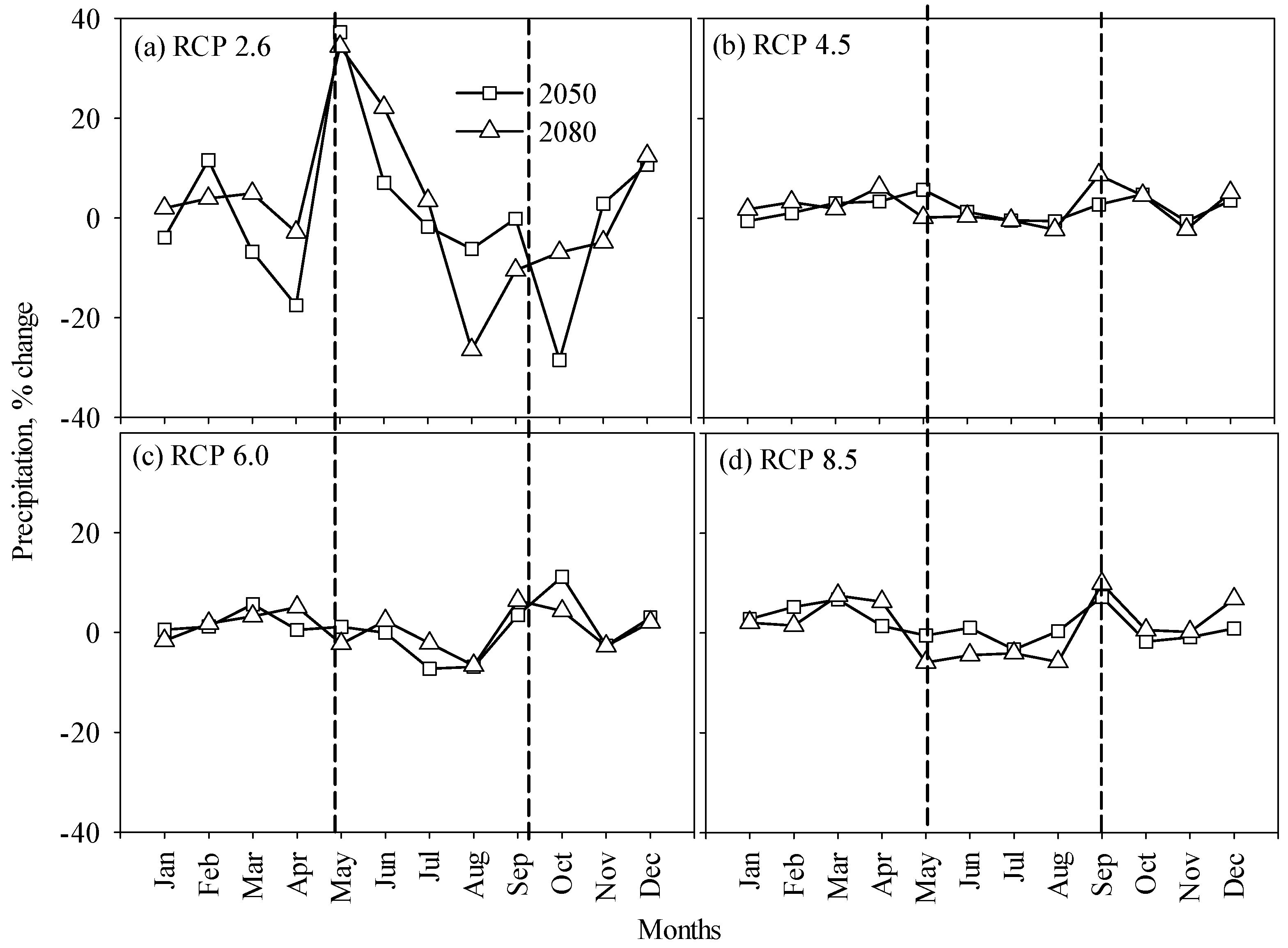
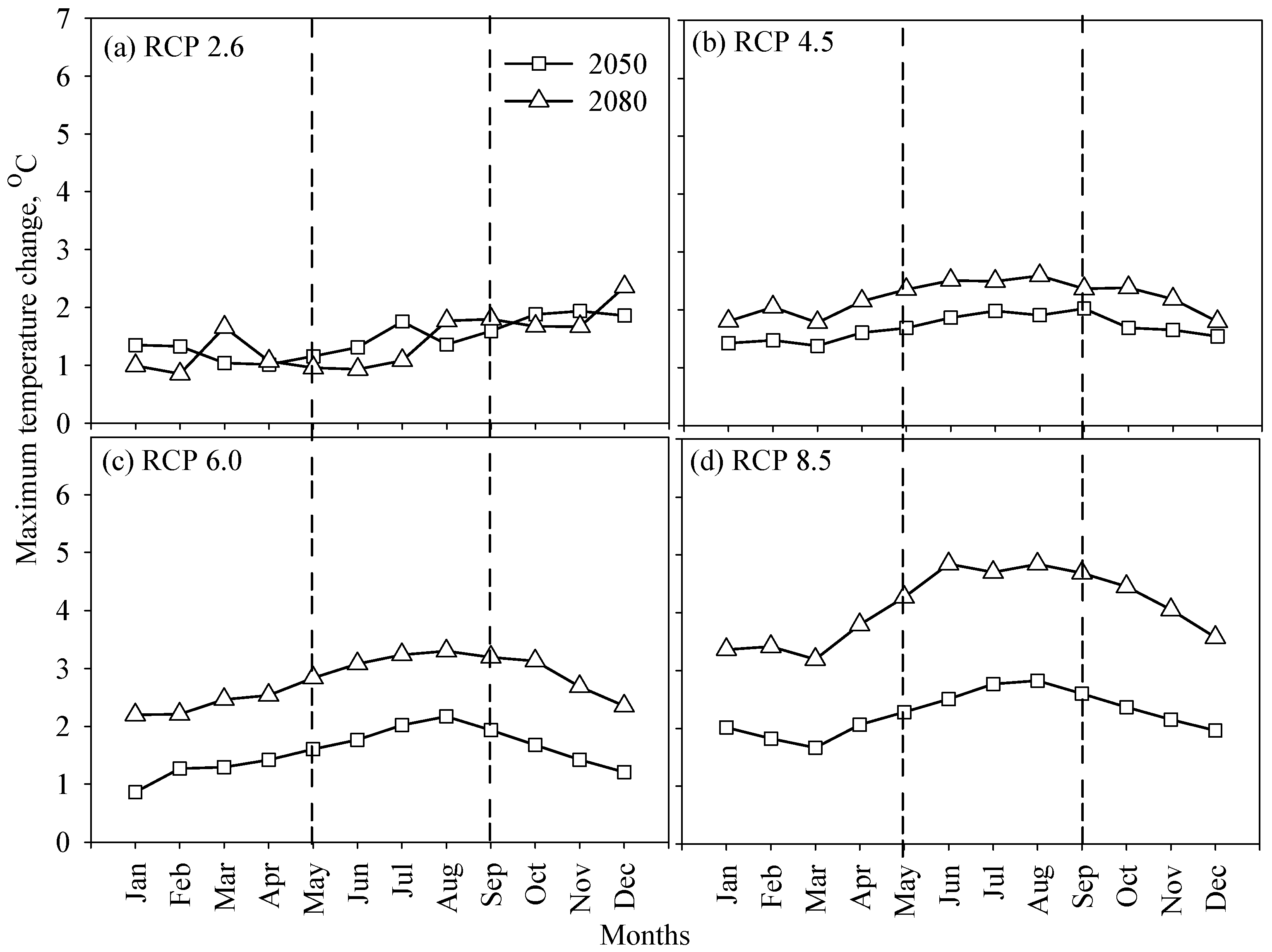
3.1. Climate Change Scenarios for the Location

The normal cotton growth season in the MS Delta region extends from about the beginning of the month of May until the end of October. The downscaled CC scenarios for average monthly rainfall and monthly averaged daily air-temperature, under RCPs of 2.6, 4.5, 6.0, and 8.5 for Stoneville differed significantly from the climate in the year 2000 (Figure 2, Figure 3 and Figure 4). The CC scenarios under all the RCPs showed month-to-month variations in amounts of rainfall and air temperature changes. The rainfall changes under RCP 2.6 showed higher variabilities compared to temperature and rainfall changes under other RCPs (4.5, 6.0, and 8.5; Figure 2a). For example, under RCP 2.6 in 2050, rainfall was projected to increase by 37% in the month of May and decrease by 28% in the month of October. However, such enhanced variability in the rainfall scenario in response to this RCP was not reflected in the case of air temperature (both maximum and minimum; Figure 3 and Figure 4). Otherwise, in all the CC scenarios in response to the remaining three RCPs, on a cotton crop-seasonal average basis, rainfall fluctuated only between −1% and 2% (Figure 2a–d).

During the cotton growth season, under the CC scenario in response to RCP 2.6, monthly averaged daily maximum temperature increases in 2050 were between 1.2 and 1.9 °C and minimum temperature between 0.6 and 1.1 °C. In 2080, the maximum temperature increases were between 0.9 and 1.8 °C and minimum temperature increases were between 0.6 and 1.3 °C across the months (Figure 3a and Figure 4a). The slight decreases in temperatures in 2080 compared to 2050 were due to the one GHG mitigation scenario applied in the RCP 2.6 pathway, which helped to reverse the warming trend in the later part of the century [59]. In the CC in response to the RCP 4.5 scenario, maximum temperature increases were between 1.7 and 2.0 °C in 2050, and between 2.4 and 2.6 °C in 2080; minimum temperature increases were between 1.5 and 1.9 °C in 2050, and 2.0 and 2.4 °C in 2080 (Figure 3b and Figure 4b). Under RCP 6.0, averaged across the crop season, maximum temperature increase was 1.9 °C in 2050, and 3.1 °C in 2080, and the average minimum temperature increase was 1.5 °C in 2050 and 2.7 °C in 2080 (Figure 3c and Figure 4c). Under the CC in response to RCP 8.5, on average, the maximum temperature increased by 2.6 and 4.6 °C in 2050 and 2080, respectively, and the minimum temperature by 2.4 and 4.4 °C, respectively (Figure 3d and Figure 4d).

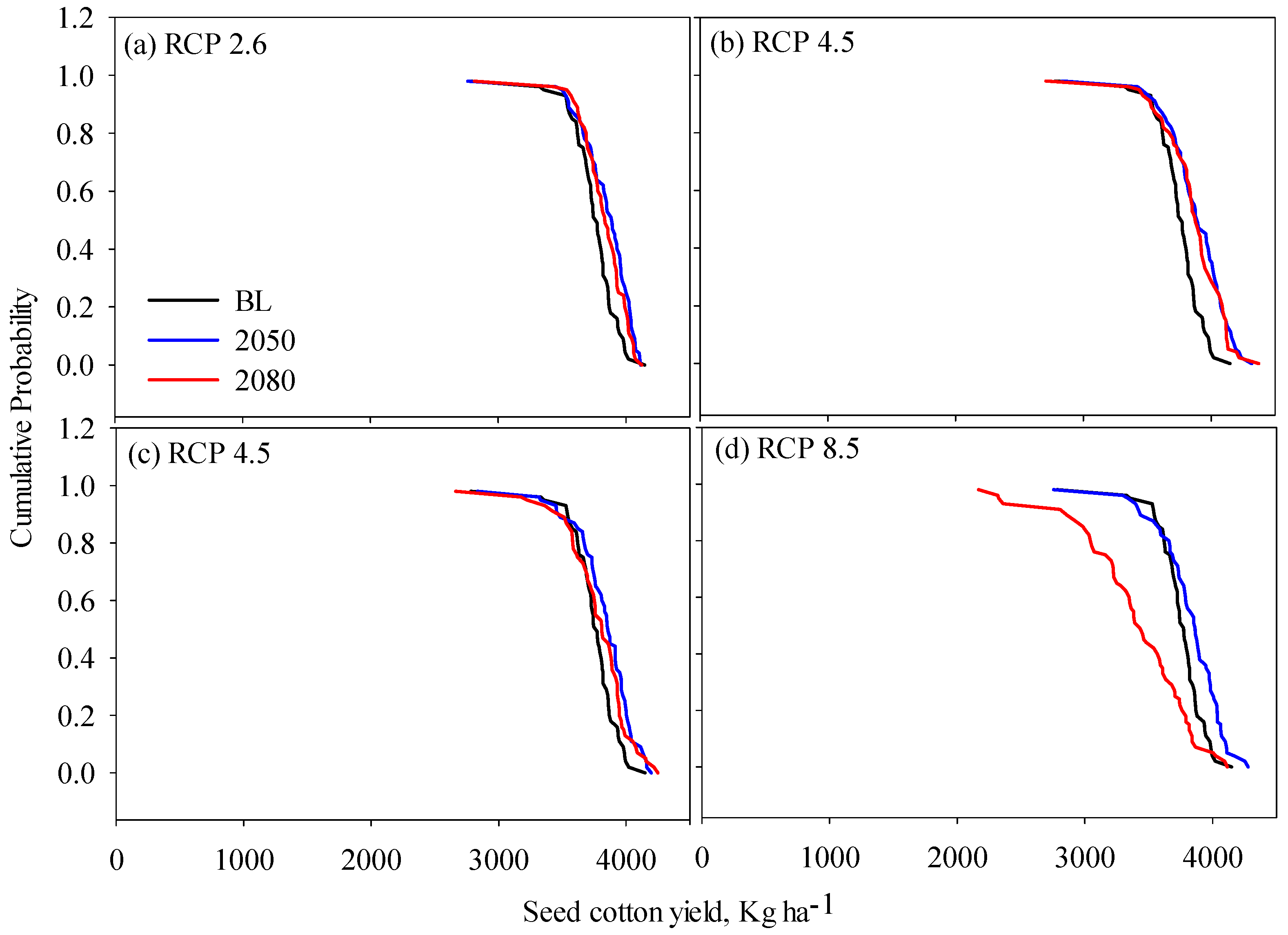
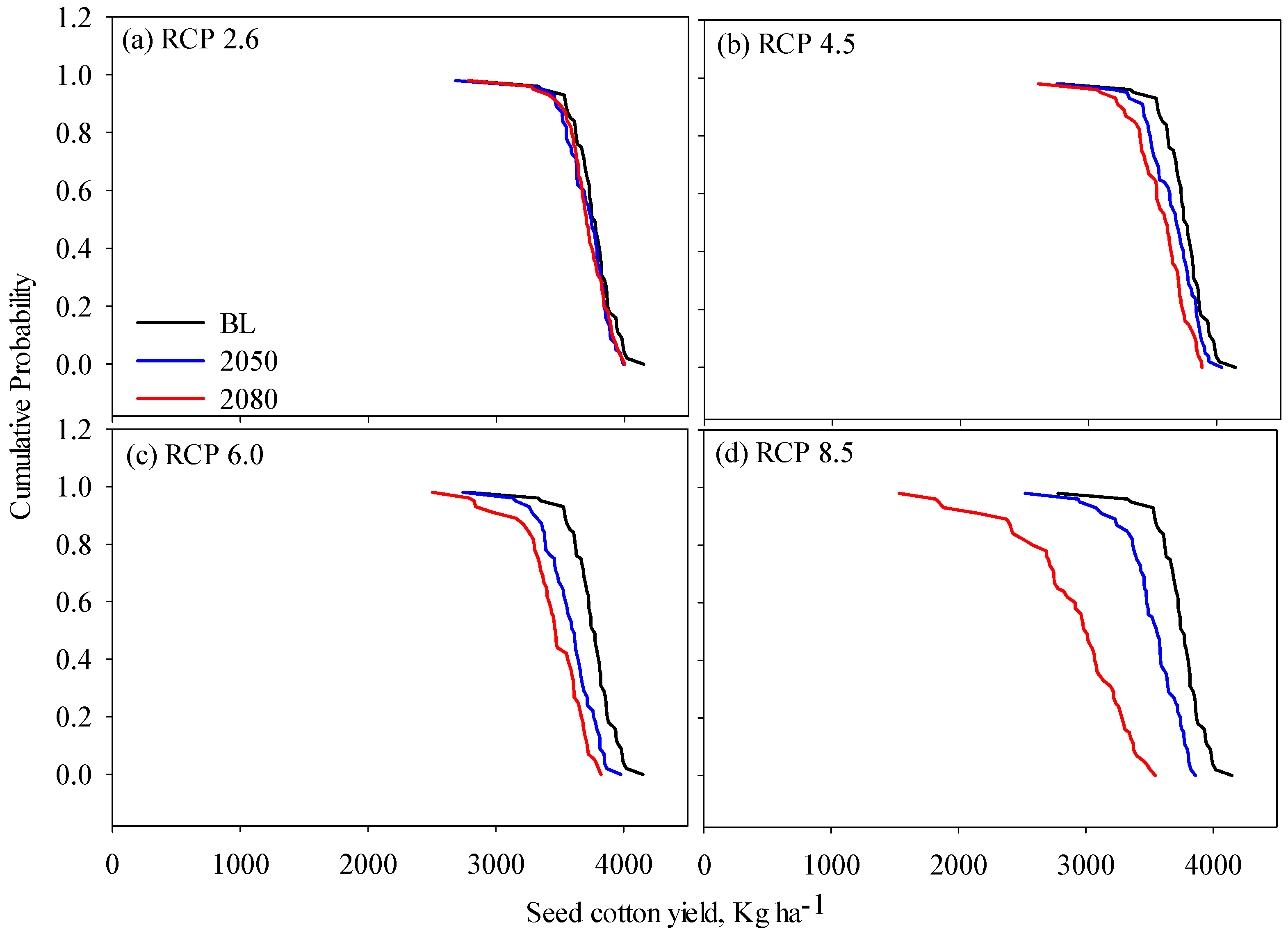
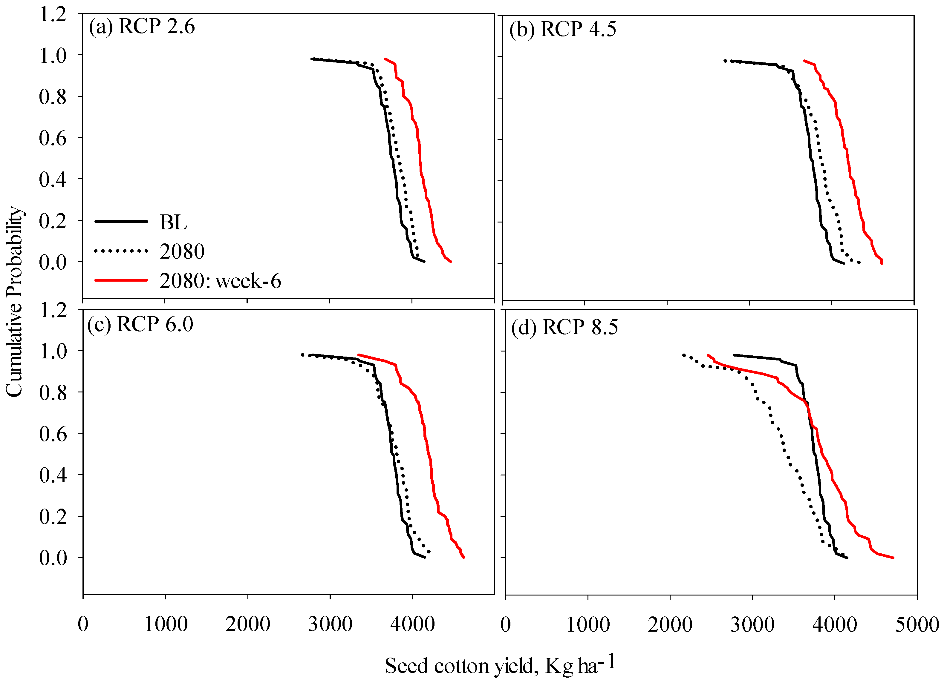
3.2. CC Impacts on Irrigated Cotton Production

Under irrigated conditions, in general, compared to the BL climate seed cotton production showed a small increase under the CC scenarios (Figure 5a–c). In 2050, the average increase in yields was 3%, 4%, and 2%, respectively, under the RCPs 2.5, 4.5, and 6.0. Under the CC scenario in response to RCP 8.5, yield still increased by 2% up to 2050, but then it declined to end with a 10% reduction compared to the BL climate in 2080 (Figure 5d). In Figure 5, Figure 6 and Figure 7, the cumulative probabilities plotted on the y-axes are created by ordering seed cotton yields over 56 years (1960–2015) so that highest yields have the lowest cumulative probability and vice versa. Hence, for a given yield on the x-axis (imagine a vertical line from this point) the curve on the right relative to another curve in the Figure represent higher probabilities of achieving the same yield. Farmers and policy makers can use these probability distributions as risk assessment tools as they anticipate changes in cotton yield production with climate change in years 2050 and 2080 relative to the BL climate.

In irrigated cotton, CO₂ concentration changes in the atmosphere alone (maximum and minimum temperature and rainfall changes were assumed to remain as in the BL climate) were found to increase simulated cotton yields steadily from the BL climate to all the CC scenarios in response to RCP 2.6 to RCP 8.5 in 2050 to 2080, except for the case of RCP 2.6 from 2050 to 2080 (Figure 6a–d). Relative to the BL climate, the changes in yield due to changes in CO₂ concentration alone in the four RCP levels were 4%, 6%, 6%, and 7% in 2050 and 4%, 7%, 9%, and 10% in 2080, respectively. When the projected temperatures associated with the CC in response to the RCPs were applied alone in the crop model simulations, on average, the yields declined by 1%, 2%, 5%, and 6% in 2050 and 1%, 5%, 8%, and 22% in 2080, respectively (Figure 7a–d). While the yield declines due to elevated atmospheric temperatures can be attributed to their effects on both photosynthesis and phenological growth stages (effectively reducing the cotton seed and boll growth duration—the time the crop takes to complete different growth stages), in the current simulations, the effect of phenology dominated over photosynthesis (Figure 8a–d). On average, in 2050, crop duration decreased by 6%, 8%, 10%, and 10% due to increased temperature in response to RCPs 2.5, 4.0, 6.0, and 8.5, respectively. Similar decreases in crop duration in 2080 were 6%, 10%, 11%, and 14%, respectively. Shortened crop duration leaves the crop with fewer days to accumulate dry-matter in seeds and fibers before the crop matures and, hence, lessened the yield return at harvest.

The enhancement in photosynthesis response in crop plants to increased CO₂ concentration in the air is termed a “fertilization effect”, and this effect can be more pronounced in a C₃ plant like cotton, compared to other C₄ plants [60]. Our simulations showed that the adverse effect of temperature on cotton yields (reduction in crop period, photosynthesis, and leaf expansion growth) either fully canceled or exceeded this fertilization effect of CO₂ on cotton growth in all the CC scenarios in response to RCPs 2.6, 4.5, and 6.0 in both 2050 and 2080, but only in 2050 under the CC scenario in response to RCP 8.5. Under the CC scenario in 2080 in response to RCP 8.5, the adverse effect of temperature superseded the fertilization effect of CO₂ in cotton growth, resulting in a net yield loss of 10% from the BL climate. Using statistical approaches and modeling Schlenker and Roberts [11] predicted that cotton has the potential of losing yield of approximately 36%–40% under CC driven by low GHG emission (B1) scenario, and 63%–70% under a high emission scenario (A1F1). However, they considered neither the positive effects of CO₂ fertilization on the photosynthesis processes nor the impacts of irrigation management on yield returns in cotton in their analyses.

Normally, enhancements in demand for water due to increasing temperatures (under the projected CC scenarios) are expected, as temperature is one of the main driving factors for evaporative water losses in the earth-atmospheric system. Notwithstanding, the enhancement in ET demand due to rise in temperature were compensated for by reductions in the total crop duration in the field (Figure 8a–d), bringing seasonal crop ET demand and, hence, total-crop-season irrigation water requirements to levels that may be less than the BL climate scenario. In the CC scenarios in response to RCPs 2.6, 4.5, 6.0, and 8.5, the changes in seasonal irrigation requirements in all the CC scenarios in response to the four RCPs in both 2050 and 2080 were found to vary only between −1% and 3%. Also, conspicuous was the decline in the seasonal ET demands with time from 2050 to 2080 in all the CC scenarios, excepting the climate in response to RCP 2.6 in 2080, in which, as expected, ET increased by a half percent compared to the BL scenario. The reasons were that the RCP 2.6 scenario included one mitigation scenario leading to a very low radiation forcing level (2.6 W·m⁻²) at the end of 2080, and the predicted CO₂ concentration levels under this RCP for 2080 (430.9 ppm) were also lower than 2050 (441.9 ppm), and the projected maximum and minimum temperatures also dropped in 2080 relative to 2050. The increase in yield due to CO₂ increase (alone, keeping other variables constant) under RCP 2.6 was 4% in the year 2080 against the increase in yield of 5% in 2050 (Figure 6a).

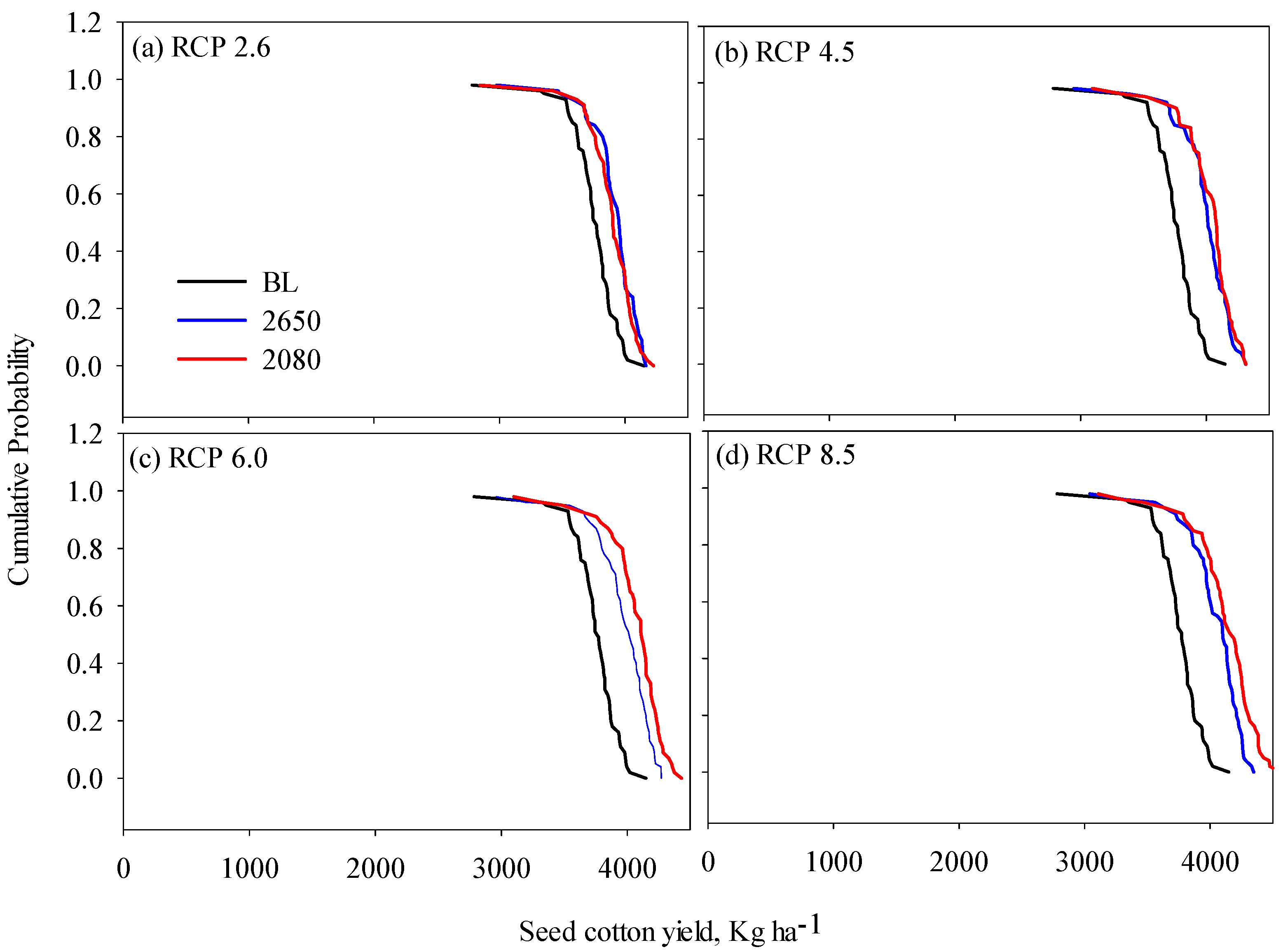
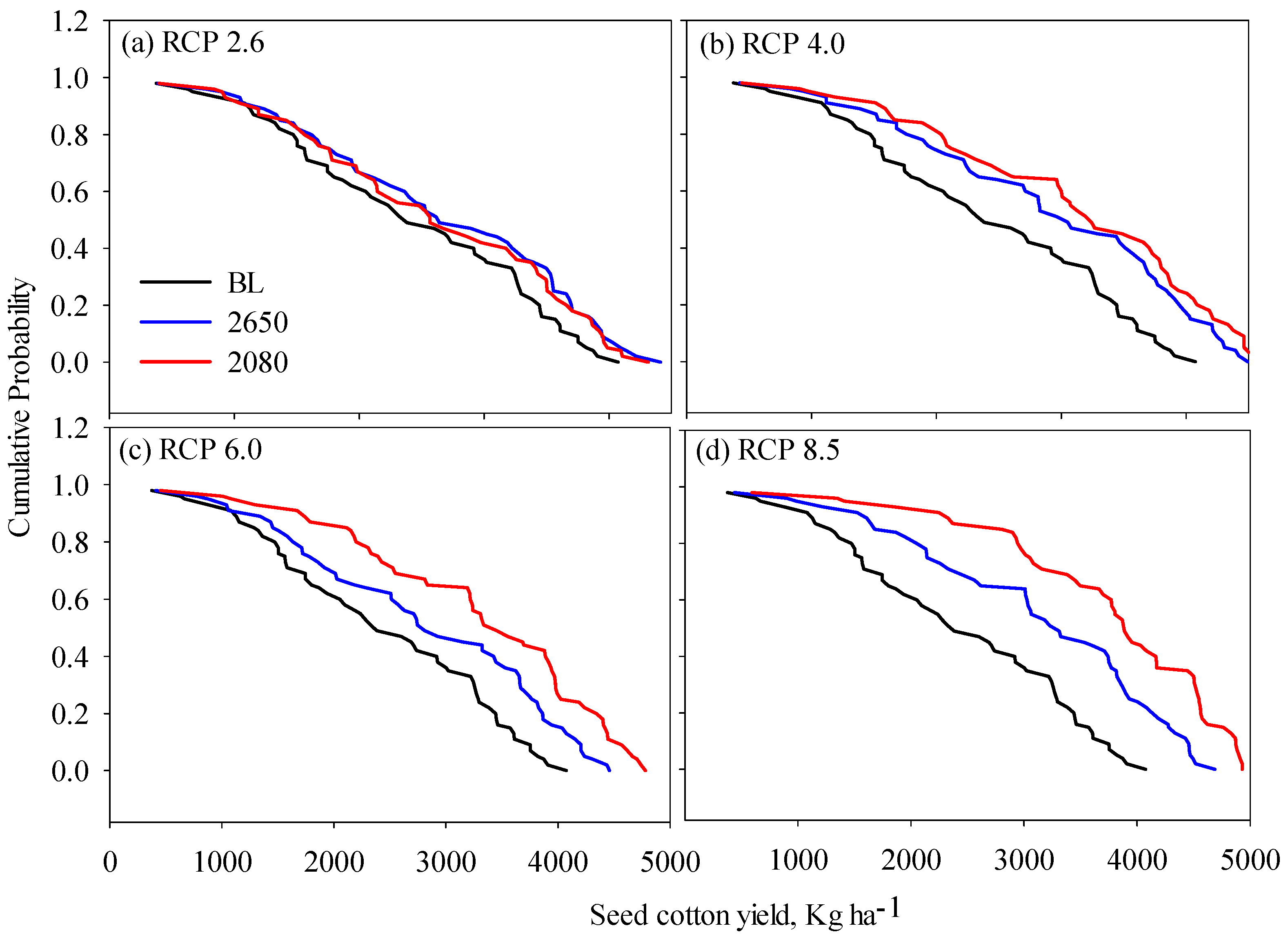
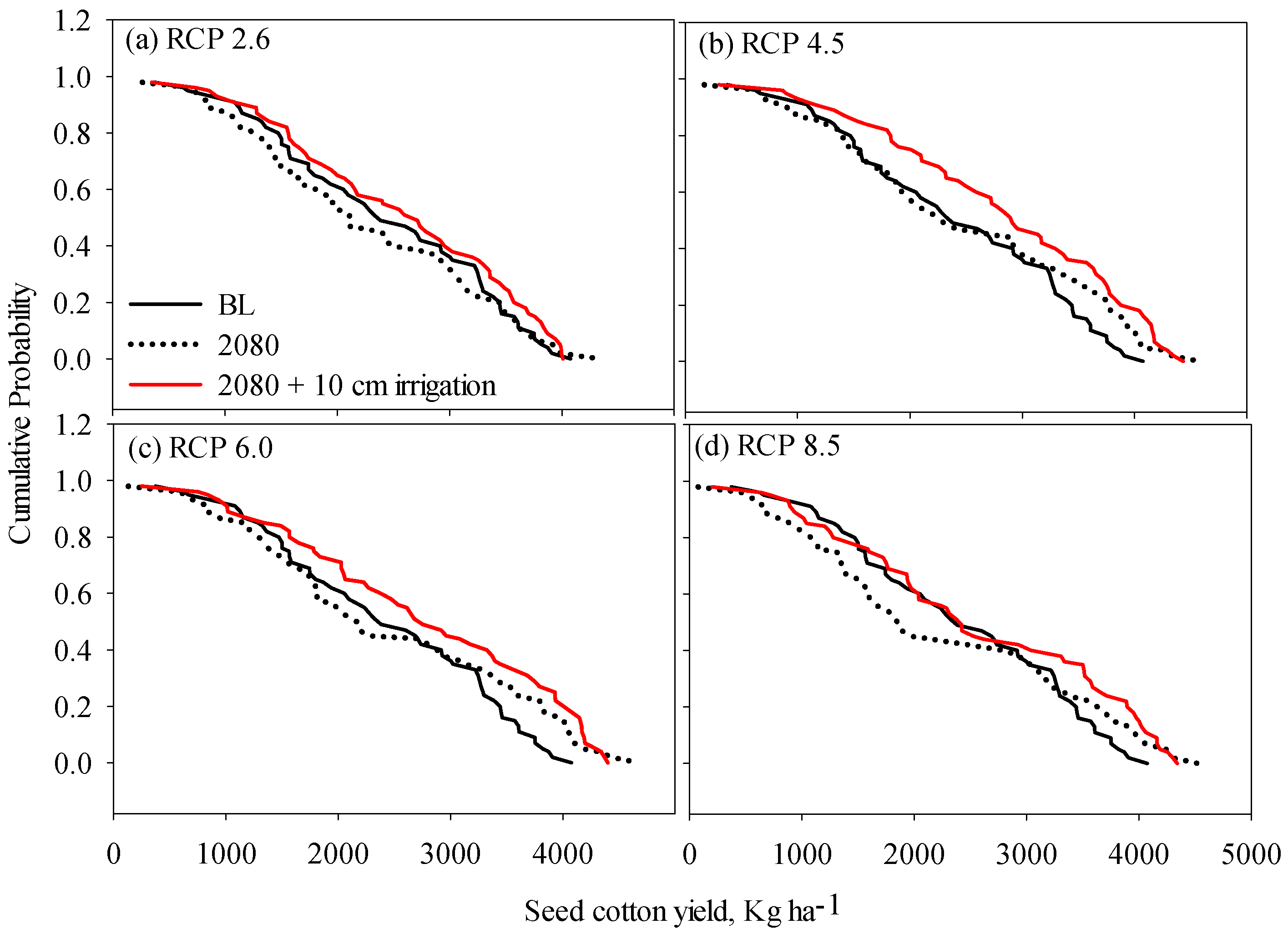
3.3. CC Effects on Rainfed Cotton Production

In general, average rainfed cotton yields declined significantly under all the CC scenarios (combined effects of changes in rainfall, temperature, and CO₂) in response to RCPs 2.5, 4.5, 6.0, and 8.5 (Figure 9a–d) in both 2050 and 2080. Under the CC in response to RCP 2.6, the yield reductions were more or less uniform across the range of yields simulated (375 to 4050 kg·ha⁻¹) (Figure 9a), however, under the CC scenarios in response to RCPs 4.5, 6.0, and 8.5, yields declined at the lower-end of the simulated yield spectrum (low-yield in response to low rainfall) and enhanced at higher-end of the simulated yield spectrum (high-yield in response to higher rainfall; Figure 9b–d). On average, in response to RCP 2.6, yields were reduced by 3% in 2050 and 6% in 2080. Similarly, the simulated yields were also reduced by 4% in 2050 under the CC in response to RCP 6.0, and by 7% under the CC in 2080 in response RCP 8.5. However, yield increased, on average, by 2% in 2050 and 3% in 2080 under the CC in response to RCP 4.5.

The simulated variability in yield, basically, reflected the recorded inter-annual variability in rainfall at the location. However, on the higher side of the yield spectrum produced in response to years with higher rainfall (water availability) for crop growth, yields simulated under the CC in response to RCPs 4.5, 6.0, and 8.5 in both 2050 and 2080 were higher than crop seasons with lower rainfall (Figure 9b–d). The higher yield responses in higher rainfall years were observed when the higher water demand for sustaining enhanced growth due to higher CO₂ in the air was supported by higher water availability from the rainfall received. Compared to the BL climate, averaged across the spectrum of yields, yields in response to rainfall were higher by 3% each under CC in response to RCP 4.5 in 2050 and 2080, and 1% each under CC in response to RCP 6.0 in 2080 and in response to RCP 8.0 in 2050.

Simulations of the crop with elevated CO₂ concentrations in the atmosphere alone, keeping temperature and rainfall at the BL climate scenario level, resulted in an increase in yields of 11%, 20%, 19%, and 29% above the BL scenario in 2050 in response to RCPs 2.6, 4.5, 6.0, and 8.5, respectively (Figure 10a–d). In 2080, a similar increase in yields under the CC scenarios in response to the four RCPs were 8%, 28%, 35%, and 54%. Notwithstanding, these yield increases were canceled by decreasing yield levels due to the temperature increases (Figure 9a–d and Figure 11a–d). The yield decreases were 14%, 17%, 18%, and 26% below the BL climate scenario in 2050, and 13%, 23%, 31%, and 49% below the BL climate scenario in 2080 under the CC scenarios in response to the four RCPs, respectively. The contribution of the projected rainfall changes under the CC scenarios in response to the four RCPs to the rainfed cotton yield reductions in both 2050 and 2080 were negligible (Figure 12a–d). Therefore, under the CC scenarios, the reduction in rainfed yield can mainly be attributed to the yield reductions due to the enhanced temperatures that affected both the crop photosynthesis and phenology growths over and above the possible yield enhancements from the CO₂ fertilization effect on photosynthesis.

Compared to the BL climate scenario, the CC scenarios in response to RCPs 2.5, 4.0, 6.0, and 8.5, resulted in less ET loss from the crop; in 2050, ET demand was less by 2%, 4%, 5%, and 6%, and in 2080, the ET demands were reduced by 1%, 6%, 7%, and 10%, respectively, than under the BL climate. While the instantaneous (daily time-step) ET demand increased with increasing temperature, the observed reduction in the ET demands was due to the significant reduction in the number of days required for the crop to mature under the CC scenarios compared to the BL climate (Figure 8a–d).

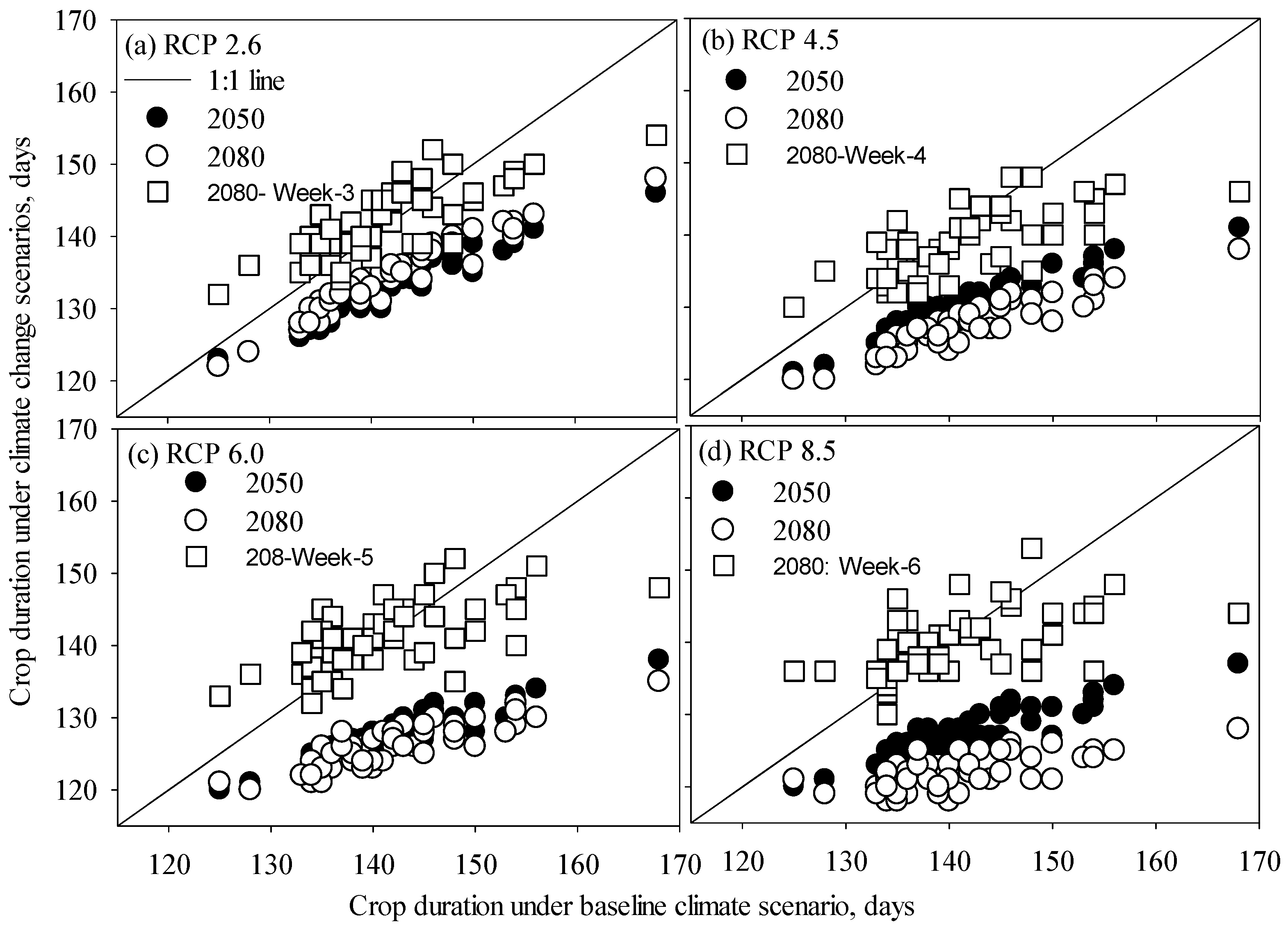
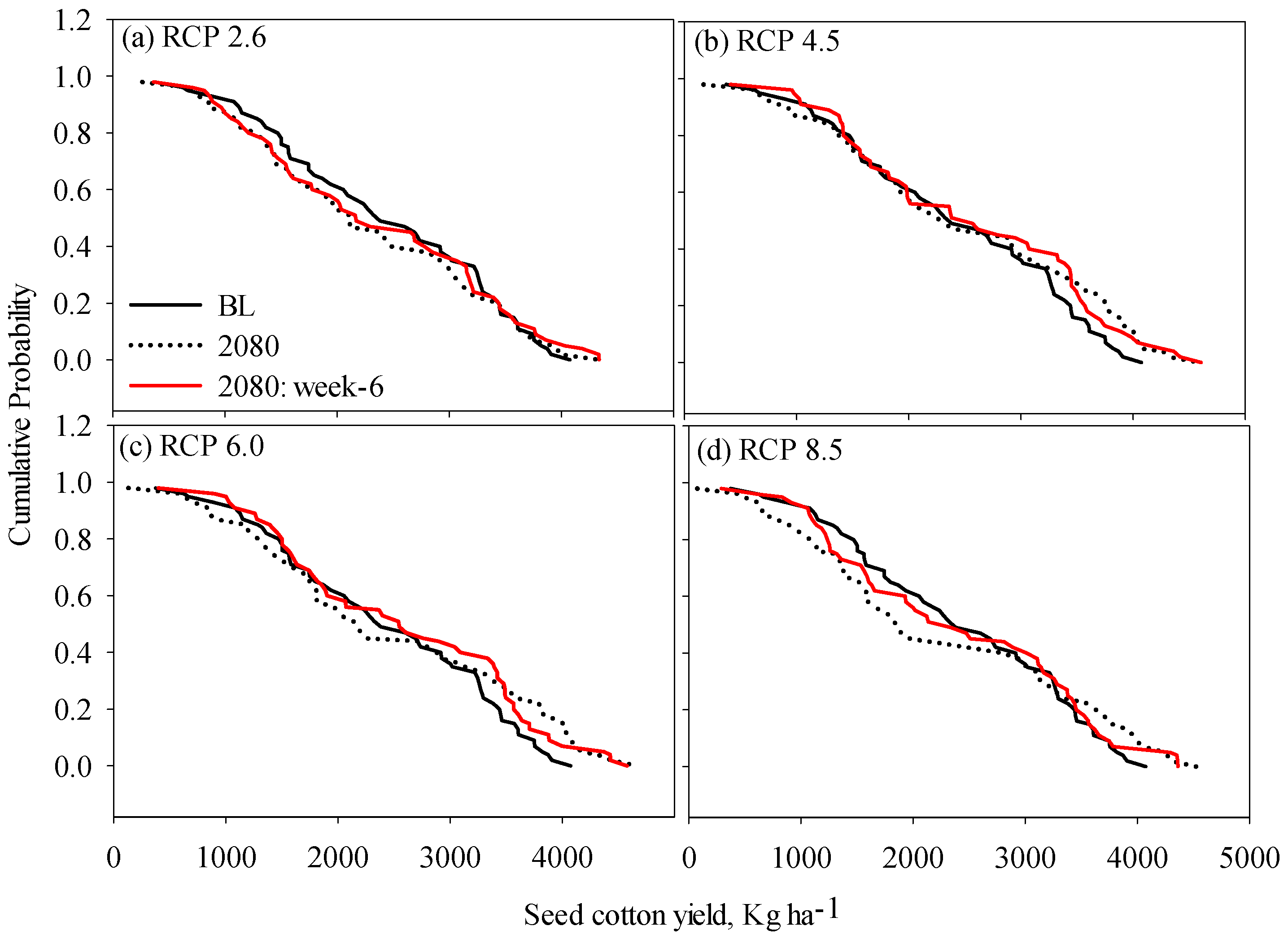
3.4. Adapting Rainfed and Irrigated Cotton to Climate Change Effects

As discussed above, the rising temperature associated with the CC scenarios across the four RCPs carry the potential for decreasing the crop growth period substantially (Figure 8a–d). There were losses in yields from increased temperatures above the optimum for the cotton growth (29–32 °C) and numerous increases above the critical limit for yield growth, 34 °C. In 2080, the fertilization effect of enhanced CO₂ concentration on photosynthesis compensated for the loss of yield due to the enhanced temperature under irrigated conditions under the RCPs 2.6, 4.5, and 6.0. However, the compensating effects of CO₂ fell short of the adverse effects of temperature on cotton growth under the CC scenario in response to RCP 8.5 (Figure 5d). Therefore, as a first adaption strategy, for the year 2080, we simulated the crop in the 10-week period immediately preceding the normal planting date of 2 May and looked for the week in which to plant for achieving the crop growth duration coinciding with the current BL climate. We observed that plantings 3, 4, 5, and 6 weeks before the normal planting date, respectively, under climates in response to RCPs 2.6, 4.5, 6.0, and 8.5, on average, produced crop durations similar to the current BL climate (Figure 8a–d). As the phenological growth of the crop was not drastically affected by water availability levels in the humid climate of the MS Delta region, these results did not differ between the rainfed and irrigated cotton growth regimes.

Under irrigated conditions, planting six weeks before the normal planting date, on average, compensated for the yield loss due to CC in response to the four RCPs (Figure 13a–d). The six-week earlier plantings, compared to normal planting, resulted in average seed cotton yield gains of 9%, 12%, 11%, and 2% under the CCs in response to the four RCPs, respectively. Notwithstanding, under the CC in response to RCP 8.5, in 25% of the years the simulated grain yields still remained below the BL climate level (Figure 13d). Earlier plantings before the six-week period or increase in fertilizer or water inputs did not compensate for this effect. Therefore, in the event of a CO₂ raise at this RCP level, the realized climate will cause cotton yield loss in 25% of the years it is planted, irrespective of adaptation measures of earlier planting.

In 2080, under rainfed conditions, planting six weeks before the normal planting date resulted in marginal yield rises of 6% each under CC scenarios in response to RCP 4.5 and 6.0 (Figure 14a–d). However, similar plantings under the CC scenarios in response to RCP 2.6 and 8.5 still produced yield declines of 3% and 2%, respectively. As an adaptation strategy, we investigated if the yield losses under the CCs can be compensated by providing irrigation water, and found that irrigating the crop with at least 10 cm of water to supplement the water available through rainfall for crop growth can boost seed cotton yield, on average, by 7%, 19%, 15%, and 8% over the baseline (BL) climate yield (Figure 15a–d).

4. Conclusions

Climate change scenarios for 2050 and 2080 were downscaled for the Mississippi Delta region from the bias-corrected and spatially disaggregated (BCSD) projections from the World Climate Research Program’s (WRCP) Coupled Model Inter-comparison and Improvement Program phase 5 (CMIP5), that informed IPCC Fifth Assessment Report (IPCC AR5) climate projections archive. Under the CC with GHG emissions corresponding to the RCPs 2.6, 4.5, 6.0, and 8.5, the air temperatures (both maximum and minimum) over the MS Delta region increased substantially in years 2050 and 2080. Rainfall changes were small. From our investigations on the possible impacts of the CC on irrigated cotton in the region, we conclude that in both 2050 and 2080, climates under emission scenarios of RCP 2.6, 4.5, and 6.0, and in 2050 under RCP 8.5, did not adversely impact seed cotton yield in the MS Delta, as the negative effects of temperature on crop growth were compensated by the positive effects of CO₂ increase on cotton growth, in spite of a reduction in growth duration caused by increased temperature. However, in the CC scenario in response to the highest emission level of RCP 8.5 in 2080, severe yield reductions are expected due to the projected increase in temperature that were not compensated by the positive effects of CO₂. In contrast, under the rainfed scenario, cotton yield declined slightly under all the four emission scenarios in both 2050 and 2080. The rainfall did not seem to provide enough plant-available water to benefit from the CO₂ fertilization effect as observed in the irrigated cotton production scenarios; however, yield still increased when the received rainfall was sufficient to meet the water requirements of the crop (in about 25% of the cases). Planting cotton six weeks in advance of the normal day of planting compensated for the yield loss due to shorter crop growing period by increased temperature under the projected CC scenarios. This early planting partially (in 75% of the years) compensated for the irrigated cotton yield loss in 2080 under RCP 8.5 and boosted yield under the CC under RCPs 2.6, 4.5, and 6.0. However, early planting under rainfed conditions failed to compensate for the rainfed cotton yield loss under the CC in both 2050 and 2080 in response to the four RCPs. Providing a “life-saving” irrigation of 10 cm compensated for this yield loss.

References

1. Solomon, S.; Qin, D.; Manning, M.; Chen, Z.; Marquis, M.; Averyt, K.B.; Tignor, M.; Miller, H.L. Climate Change 2007: The Physical Science Basis. Contribution of Working Group I to the Fourth Assessment Report of the Intergovernmental Panel on Climate Change; Cambridge University Press: Cambridge, UK; New York, NY, USA, 2007. [Google Scholar]
2. Tans, P.; Keeling, R. Trends in Atmospheric CO2 at Mauna Loa, Hawaii NOAA Earth System Research Laboratory. Available online: http://www.esrl.noaa.gov/gmd/ccgg/trends/ (accessed on 26 October 2016).
3. Field, C.B.; Barros, V.R.; Dokken, D.J.; Mach, K.J.; Mastrandrea, M.D.; Bilir, T.E.; Chatterjee, M.; Ebi, K.L.; Estrada, Y.O.; Genova, R.C.; et al. Climate Change 2014: Impacts, Adaptation, and Vulnerability. The Contribution of Working Group II to the Fifth Assessment Report of the Intergovernmental Panel on Climate Change; Cambridge University Press: Cambridge, UK; New York, NY, USA, 2014. [Google Scholar]
4. Liebig, M.A.; Franzluebbers, A.J.; Follett, R.F. Agriculture and climate change: Mitigation opportunities and adaptation imperatives. In Managing Agricultural Greenhouse Gases: Coordinated Agricultural Research through GRACEnet to Address Our Changing Climate; Liebig, M.A., Franzluebbers, A.J., Follett, R.F., Eds.; Academic Press: New York, NY, USA, 2012; pp. 3–11. [Google Scholar]
5. Aeschbach-Hertig, W.; Gleeson, T. Regional strategies for the accelerating global problem of groundwater depletion. Nat. Geosci. 2012, 5, 853–861. [Google Scholar] [CrossRef]
6. Gurdak, J.J.; Qi, S.L. Vulnerability of recently recharged groundwater in principle aquifers of the United States to nitrate contamination. Environ. Sci. Technol. 2012, 46, 6004–6012. [Google Scholar] [CrossRef] [PubMed]
7. Dijkstra, F.A.; Blumenthal, D.; Morgan, J.A.; Pendall, E.; Carrillo, Y.; Follett, R.F. Contrasting effects of elevated CO2 and warming on nitrogen cycling in a semiarid grassland. New Phytol. 2010, 187, 426–437. [Google Scholar] [CrossRef] [PubMed]
8. White, J.W.; Hoogenboom, G.; Kimball, B.A.; Wall, G.W. Methodologies for simulating impacts of climate change on crop production. Field Crop. Res. 2011, 124, 357–368. [Google Scholar] [CrossRef]
9. Reddy, V.R.; Baker, D.N.; Hodges, H.F. Temperature effect on cotton canopy growth, photosynthesis and respiration. Agron. J. 1991, 83, 699–704. [Google Scholar] [CrossRef]
10. Reddy, K.R.; Hodges, H.F.; McKinion, J.M. A comparison of scenarios for the effect of global climate change on cotton growth and yield. Aust. J. Plant Physiol. 1997, 24, 707–713. [Google Scholar] [CrossRef]
11. Schlenker, W.; Roberts, M.J. Nonlinear temperature effects indicate severe damages to yields under climate change. Proc. Natl. Acad. Sci. USA 2009, 106, 15594–15598. [Google Scholar] [CrossRef] [PubMed]
12. Hatfield, J.L.; Boote, K.J.; Kimball, B.A.; Ziska, L.H.; Izaurralde, R.C.; Ort, D.; Thomson, A.M.; Wolfe, D.W. Climate impacts on agriculture: Implications for crop production. Agron. J. 2011, 103, 351–370. [Google Scholar] [CrossRef]
13. Reddy, V.R.; Hodges, H.F.; McCarty, W.H.; McKinnon, J.M. Weather and Cotton Growth: Present and Future; Mississippi State University: Starkeville, MS, USA, 1996. [Google Scholar]
14. Reddy, V.R.; Reddy, K.R.; Hodges, H.F. Carbon dioxide enrichment and temperature effects on cotton canopy photosynthesis, transpiration, and water use efficiency. Field Crop. Res. 1995, 41, 13–23. [Google Scholar] [CrossRef]
15. Saseendran, S.A.; Singh, K.K.; Rathore, L.S.; Singh, S.V.; Sinha, S.K. Effects of climate change on rice production in Kerala. Clim. Chang. 2000, 44, 495–514. [Google Scholar] [CrossRef]
16. Rosenzweig, C.; Tubiello, F.N. Effects of changes in minimum and maximum temperature on wheat yields in the central US: A simulation study. Agric. For. Meteorol. 1996, 80, 215–230. [Google Scholar] [CrossRef]
17. Rosenzweig, C.; Allen, L.H., Jr.; Jones, J.W.; Tsuji, G.Y.; Hildebrand, P. Climate Change and Agriculture: Analysis of Potential International Impacts (ASA Special Publication No. 59); American Society of Agronomy, Inc.: Madison, WI, USA, 1995. [Google Scholar]
18. Bassu, S.; Asseng, S.; Richards, R. Yield benefits of triticale traits for wheat under current and future climates. Field Crop. Res. 2011, 124, 14–24. [Google Scholar] [CrossRef]
19. Gouache, D.; Le Bris, X.; Bogard, M.; Deudon, O.; Pagé, C.; Gate, P. Evaluating agronomic adaptation options to increasing heat stress under climate change during wheat grain filling in France. Eur. J. Agron. 2012, 39, 62–70. [Google Scholar] [CrossRef]
20. Teixeira, E.I.; Fischer, G.; van Velthuizen, H.; Walter, C.; Ewert, F. Global hot-spots of heat stress on agricultural crops due to climate change. Agric. For. Meteorol. 2013, 170, 206–215. [Google Scholar] [CrossRef]
21. Deryng, D.; Conway, D.; Ramankutty, N.; Price, J.; Warren, R. Global crop yield response to extreme heat stress under multiple climate change futures. Environ. Res. Lett. 2014, 9, 034011. [Google Scholar] [CrossRef]
22. Moriondo, M.; Giannakopoulos, C.; Bindi, M. Climate change impact assessment: The role of climate extremes in crop yield simulation. Clim. Chang. 2011, 104, 679–701. [Google Scholar] [CrossRef]
23. Gaiser, T.; Perkons, U.; Küpper, P.M.; Kautz, T.; Uteau-Puschmann, D.; Ewert, F.; Enders, A.; Krauss, G. Modeling biopore effects on root growth and biomass production on soils with pronounced sub-soil clay accumulation. Ecol. Model. 2013, 256, 6–15. [Google Scholar] [CrossRef]
24. Ahuja, L.R.; Rojas, K.W.; Hanson, J.D.; Shafer, M.J.; Ma, L. Root Zone Water Quality Model. Modeling Management Effects on Water Quality and Crop Production; Water Resources Publications, LLC: Highlands Ranch, CO, USA, 2000. [Google Scholar]
25. Jones, J.W.; Hoogenboom, G.; Porter, C.H.; Boote, K.J.; Batchelor, W.D.; Hunt, L.A.; Wilkens, P.W.; Singh, U.; Gijsman, A.J.; Ritchie, J.T. The DSSAT cropping system model. Eur. J. Agron. 2003, 18, 235–265. [Google Scholar] [CrossRef]
26. Islam, A.; Ahuja, L.R.; Garcia, L.A.; Ma, L.; Saseendran, S.A. Modeling the effect of elevated CO2 and climate change on reference evapotranspiration in the semi-arid great plains. Trans. ASABE 2012, 55, 2135–2146. [Google Scholar] [CrossRef]
27. Islam, A.; Ahuja, L.R.; Garcia, L.A.; Ma, L.; Saseendran, S.A.; Trout, T.J. The impacts of climate change on irrigated corn production in the Central Great Plains. Agric. Water Manag. 2012, 110, 94–108. [Google Scholar] [CrossRef]
28. Ko, J.; Ahuja, L.R.; Saseendran, S.A.; Green, T.R.; Ma, L. Simulation impacts of GCM-projected climate change on dryland cropping systems in the U.S. Central Great Plains. Agric. For. Meteorol. 2010, 150, 1331–1346. [Google Scholar]
29. Ko, J.; Ahuja, L.R.; Kimball, B.C.; Saseendran, S.A.; Ma, L.; Green, T.R.; Wall, G.; Pinter, P. Simulation of climate change impacts on cropping systems in the Central Great Plains. Clim. Chang. 2012, 111, 445–472. [Google Scholar] [CrossRef]
30. Boote, K.J.; Pickering, N.B.; Allen, L.H., Jr. Plant modeling: Advances and gaps in our capability to project future crop growth and yield in response to global climate change. In Advances in Carbon Dioxide Effects Research (Special Publication No. 61); Allen, L.H., Jr., Kirkham, M.B., Olszyk, D.M., Whitman, C.E., Eds.; ASA, CSSA, and SSSA: Madison, WI, USA, 1997; pp. 179–228. [Google Scholar]
31. Garcia y Garcia, A.; Persson, T.; Paz, J.O.; Fraisse, C.; Hoogenboom, G. ENSO-based climate variability affects water use efficiency of rainfed cotton grown in the southeastern USA. Agric. Ecosyst. Environ. 2010, 139, 629–635. [Google Scholar] [CrossRef]
32. Gérardeaux, E.; Sultan, B.; Palaï, O.; Guiziou, C.; Oettli, P.; Naudin, K. Positive effect of climate change on cotton in 2050 by CO2 enrichment and conservation agriculture in Cameroon. Agron. Sustain. Dev. 2013, 33, 485–495. [Google Scholar] [CrossRef]
33. Saseendran, S.A.; Pettigrew, W.T.; Reddy, K.N.; Ma, L.; Fisher, D.K.; Sui, R. Climate optimized planting windows for cotton in the Lower Mississippi Delta region. Agronomy 2016, 6. [Google Scholar] [CrossRef]
34. Christensen, N.S.; Lettenmaier, D.P. A multimodel ensemble approach to assessment of climate change impacts on the hydrology and water resources of the Colorado River basin. Hydrol. Earth Syst. Sci. 2007, 3, 3727–3770. [Google Scholar] [CrossRef]
35. IPCC. Summary for policymakers. In Climate Change 2014: Impacts, Adaptation, and Vulnerability. Part A: Global and Sectoral Aspects. Contribution of Working Group II to the Fifth Assessment Report of the Intergovernmental Panel on Climate Change; Field, C.B., Barros, V.R., Dokken, D.J., Mach, K.J., Mastrandrea, M.D., Bilir, T.E., Chatterjee, M., Ebi, K.L., Estrada, Y.O., Genova, R.C., et al., Eds.; Cambridge University Press: Cambridge, UK; New York, NY, USA, 2014; pp. 1–32. [Google Scholar]
36. Shukla, J.; DelSole, T.; Fennessy, M.; Kinter, J.; Paolino, D. Climate model fidelity and projections of climate change. Geophys. Res. Lett. 2006, 33, L07702. [Google Scholar] [CrossRef]
37. Giorgi, F.; Mearns, L. Calculation of average, uncertainty range and reliability of regional climate changes from AOGCM simulations via the ‘reliability ensemble averaging’ (REA) method. J. Clim. 2002, 15, 1141–1158. [Google Scholar] [CrossRef]
38. IPCC. Climate Change 2007: The Scientific Basis. Contribution of Working Group I to the Fourth Assessment Report of the Intergovernmental Panel on Climate Change; Solomon, S., Ed.; Cambridge University Press: Cambridge, UK, 2007. [Google Scholar]
39. Reifen, C.; Toumi, R. Climate projections: Past performance no guarantee of future skill? Geophys. Res. Lett. 2009, 36, L13704. [Google Scholar] [CrossRef]
40. Pettigrew, W.T.; Dowd, M.K. Varying planting dates or irrigation regimes alters cottonseed composition. Crop Sci. 2011, 51, 2155–2164. [Google Scholar] [CrossRef]
41. Brooks, R.H.; Corey, A.T. Hydraulic Properties of Porous Media; Hydrology Paper 3; Colorado State University: Fort Collins, CO, USA, 1964. [Google Scholar]
42. Ahuja, L.R.; Ma, L.; Fang, Q.X.; Saseendran, S.A.; Islam, A.; Malone, R.W. Computer modeling: Applications to environment and food security. In Encyclopedia of Agriculture and Food Systems; van Alfen, N., Ed.; Elsevier: San Diego, CA, USA, 2013; pp. 337–358. [Google Scholar]
43. Ma, L.; Nielsen, D.C.; Ahuja, L.R.; Malone, R.W.; Saseendran, S.A.; Rojas, K.W.; Hanson, J.D.; Benjamin, J.G. Evaluation of RZWQM under varying irrigation levels in eastern Colorado. Trans. ASAE 2003, 46, 39–49. [Google Scholar]
44. Ma, L.; Hoogenboom, G.; Saseendran, S.A.; Bartling, P.N.S.; Ahuja, L.R.; Green, T.R. Estimates of soil hydraulic properties and root growth factor on soil water balance and crop production. Agron. J. 2009, 101, 572–583. [Google Scholar] [CrossRef]
45. Hoogenboom, G.; Jones, J.W.; Boote, K.J. A decision support system for prediction of crop yield, evapotranspiration, and irrigation management. In Proceedings of the 1991 Irrigation and Drainage, Honolulu, HI, USA, 22–26 July 1991; ASCE: Reston, VA, USA, 1991. [Google Scholar]
46. Ma, L.; Hoogenboom, G.; Ahuja, L.R.; Ascough, J.C., II; Saseendran, S. Evaluation of the RZWQM-CERES-Maize hybrid model for maize production. Agric. Syst. 2006, 87, 274–295. [Google Scholar] [CrossRef]
47. Saseendran, S.A.; Ahuja, L.R.; Nielsen, D.C.; Trout, T.J.; Ma, L. Use of crop simulation models to evaluate limited irrigation management options for corn in a semiarid environment. Water Resour. Res. 2008, 44, W00E02. [Google Scholar] [CrossRef]
48. Saseendran, S.A.; Trout, T.J.; Ahuja, L.R.; Ma, L.; McMaster, G.; Andales, A.A.; . Chaves, J.; Ham, J. Quantification of crop water stress factors from soil water measurements in limited irrigation experiments. Agric. Syst. 2015, 137, 191–205. [Google Scholar] [CrossRef]
49. Nimah, M.N.; Hanks, R.J. Model for estimating soil water, plant and atmospheric inter relations: I. description and sensitivity. Proc. Soil Sci. Soc. Am. 1973, 37, 522–527. [Google Scholar] [CrossRef]
50. Farquhar, G.D.; von Caemmerer, S.; Berry, J.A. A biochemical model of photosynthetic CO2 assimilation in leaves of C3 species. Planta 1980, 149, 78–90. [Google Scholar] [CrossRef] [PubMed]
51. Boote, K.J.; Jones, J.W.; Hoogenboom, G.; Pickering, N.B. The CROPGRO model for grain legumes. In Understanding Options for Agricultural Production; Tsuji, G.Y., Ed.; Kluwer Academic Publishers: Dordrecht, The Netherlands, 1998; pp. 99–128. [Google Scholar]
52. Farquhar, G.D.; von Caemmerer, S. Modeling of photosynthetic response to environment. In Physiological Plant Ecology II; Lange, O.L., Ed.; Springer: Berlin, Germany, 1982; pp. 549–587. [Google Scholar]
53. Pickering, N.B.; Jones, J.W.; Boote, K.J. Adapting SOYGRO V5.42 for prediction under climate change conditions. In Climate Change and Agriculture: Analysis of Potential International Impacts; Rosenzweig, C., Ed.; ASA, CSSA, and SSSA: Madison, WI, USA, 1995; pp. 77–98. [Google Scholar]
54. Alagarswamy, G.; Boote, K.J.; Allen, L.H., Jr.; Jones, J.W. Evaluating the CROPGRO-Soybean model ability to simulate photosynthesis response to carbon dioxide levels. Agron. J. 2006, 98, 34–42. [Google Scholar] [CrossRef]
55. Shuttleworth, W.J.; Wallace, J.S. Evaporation from sparse crops-an energy combination theory. Q. J. R. Meteorol. Soc. 1985, 111, 839–855. [Google Scholar] [CrossRef]
56. Allen, L.H.; Boote, K.J.; Jones, J.W.; Valle, R.R.; Acock, B.; Rogers, H.H.; Dahlman, R.C. Response of vegetation to rising carbon dioxide: Photosynthesis, biomass, and seed yield of soybean. Glob. Biochem. Cycles 1987, 1, 1–14. [Google Scholar] [CrossRef]
57. Allen, L.H. Plant responses to rising carbon dioxide and potential interactions with air pollutants. J. Environ. Qual. 1990, 19, 15–34. [Google Scholar] [CrossRef]
58. Rogers, H.H.; Bingham, G.E.; Cure, J.D.; Smith, J.M.; Suran, K.A. Responses of selected plant species to elevated carbon dioxide in the field. J. Environ. Qual. 1983, 12, 569–574. [Google Scholar] [CrossRef]
59. Van Vuuren, D.P.; Edmonds, J.; Kainuma, M.; Riahi, K.; Thomson, A.; Hibbard, K.; Hurtt, G.C.; Kram, T.; Krey, V.; Lamarque, J.F.; et al. The representative concentration pathways: An overview. Clim. Chang. 2011, 109, 5–31. [Google Scholar] [CrossRef]
60. Leakey, A.D.B.; Ainsworth, E.A.; Bernacchi, C.J.; Rogers, A.; Long, S.P.; Ort, D.R. Elevated CO2 effects on plant carbon, nitrogen, and water relations: Six important lessons from FACE. J. Exp. Bot. 2009, 60, 2859–2876. [Google Scholar] [CrossRef] [PubMed]
Figure 1. Measured and simulated seed cotton yield from normal and early plantings under rainfed (a) and irrigated (b) conditions during 2005–08 at Stoneville, MS. Error bars indicate one SD from the mean of the measured yield across the four treatment replications. RMSE = Root Mean Squared Errors. RRMSE = RMSE relative to mean values. ME = Arithmetic Mean Error.
Climate 04 00055 g001
Figure 2. Coupled Model Inter-comparison Project Phase 5 (CMIP5) multi-climate model ensemble projections of rainfall change at Stoneville, MS, for the four emissions scenarios of the Representative Concentration Pathways (RCPs), RCP 2.6 (a), 4.5 (b), 6.0 (c), and 8.5 (d), as used in the IPCC Fifth Assessment Report. Dotted lines in the vertical demarcate the normal cotton growth season (May to September).
Climate 04 00055 g002
Figure 3. Coupled Model Inter-comparison Project Phase 5 (CMIP5) multi-climate model ensemble projected maximum temperature changes at Stoneville, MS, for the four emissions scenarios of the Representative Concentration Pathways (RCPs), RCP 2.6 (a), 4.5 (b), 6.0 (c), and 8.5 (d), as used in the IPCC Fifth Assessment Report. Dotted lines in the vertical demarcate the normal cotton growth season (May to September).
Climate 04 00055 g003
Figure 4. Coupled Model Inter-comparison Project Phase 5 (CMIP5) multi-climate model ensemble projected minimum temperature change at Stoneville, MS, for the four emissions scenarios of the Representative Concentration Pathways (RCPs), RCP 2.6 (a), 4.5 (b), 6.0 (c), and 8.5 (d), as used in the IPCC Fifth Assessment Report. Dotted lines in the vertical demarcate the normal cotton growth season (May to September).
Climate 04 00055 g004
Figure 5. Simulated impacts of climate change (changes in temperature, rainfall, and CO2) on irrigated seed cotton yield in 2050 and 2080 under the four emission scenarios of RCP 2.6 (a), 4.5 (b), 6.0 (c), and 8.5 (d).
Climate 04 00055 g005
Figure 6. Simulated impacts of CO2 concentration in the air alone, under RCP 2.6 (a), 4.5 (b), 6.0 (c), and 8.5 (d) greenhouse gas (GHG) emission scenarios on irrigated seed cotton yield in 2050 and 2080. The projected temperature and rainfall changes were not considered.
Climate 04 00055 g006
Figure 7. Simulated impacts of temperature rises alone on irrigated seed cotton yield in 2050 and 2080 under RCP 2.6 (a), 4.5 (b), 6.0 (c), and 8.5 (d) greenhouse gas (GHG) scenarios. Projected changes in both maximum and minimum temperatures alone were considered assuming no CO2 and rainfall changes.
Climate 04 00055 g007
Figure 8. Comparison between the simulated crop durations in baseline climate and crop durations under climate change (CC) in 2050 and 2080 under RCPs of 2.6 (a), 4.5 (b), 6.0 (c), and 8.5 (d) for normal date of planting (2 May). Also, shown are the crop durations for earlier than normal plantings of three weeks (week-3) under RCP 2.5, four weeks (week-4) under RCP 4.5, five weeks (week-5) under RCP 6.0, and six weeks (week-6) under RCP 8.5 driven climate changes in 2080.
Climate 04 00055 g008
Figure 9. Simulated impacts of climate change (changes in temperature, rainfall, and CO2) on rainfed seed cotton yield in 2050 and 2080 for RCP 2.6 (a), 4.5 (b), 6.0 (c), and 8.5 (d) emission scenarios.
Climate 04 00055 g009
Figure 10. Simulated impacts of CO2 concentration in the air alone on rainfed seed cotton yield under RCP 2.6 (a), 4.5 (b), 6.0 (c), and 8.5 (d) emission scenarios in 2050 and 2080. The projected temperature and rainfall changes were not considered.
Climate 04 00055 g010
Figure 11. Simulated impacts of temperature rises in 2050 and 2080 alone on rainfed seed cotton yield under RCP 2.6 (a), 4.5 (b), 6.0 (c), and 8.5 (d) emission scenarios. Projected changes in both maximum and minimum temperatures alone were considered assuming no CO2 and rainfall changes.
Climate 04 00055 g011
Figure 12. Simulated impacts of rainfall changes alone in 2050 and 2080 on rainfed seed cotton yield for RCP 2.6 (a), 4.5 (b), 6.0 (c), and 8.5 (d) emission scenarios on rainfed seed cotton yield. Projected changes in both maximum and minimum temperatures and CO2 and rainfall changes were not included.
Climate 04 00055 g012
Figure 13. Comparison between the simulated irrigated seed cotton yield under baseline (BL) climate and climate change (CC; changes in CO2, temperature, and rainfall) in 2080 for RCP 2.6 (a), 4.5 (b), 6.0 (c), and 8.5 (d) for normal day of planting (2 May) and earlier than normal-day plantings of six weeks (week-6).
Climate 04 00055 g013
Figure 14. Comparison between the simulated rainfed seed cotton yield under baseline (BL) climate and climate change (CC; changes in CO2, temperature, and rainfall) in 2080 under RCP 2.6 (a), 4.5 (b), 6.0 (c), and 8.5 (d) for normal day of planting (2 May) and earlier than normal-day plantings of six weeks (week-6).
Climate 04 00055 g014
Figure 15. Comparison between the simulated rainfed seed cotton yield under baseline (BL) climate and climate change (CC; changes in CO2, temperature, and rainfall) in 2080 under RCP 2.6 (a), 4.5 (b), 6.0 (c), and 8.5 (d) for normal day of planting (2 May) with normal planting plus 10 cm irrigation.
Climate 04 00055 g015