
Assessing River Low-Flow Uncertainties Related to Hydrological Model Calibration and Structure under Climate Change Conditions

Abstract
:1. Introduction
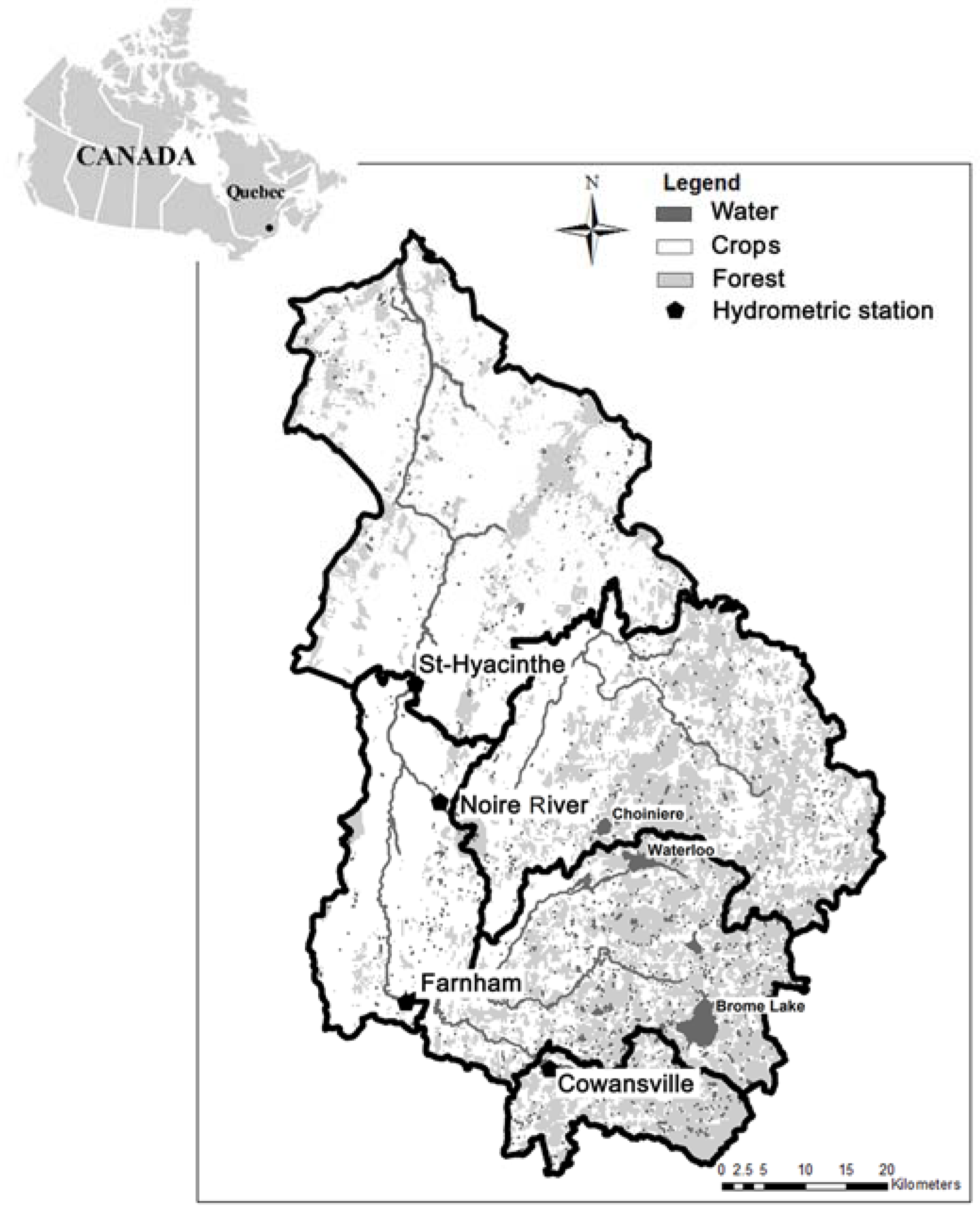
2. Study Area
3. Methods
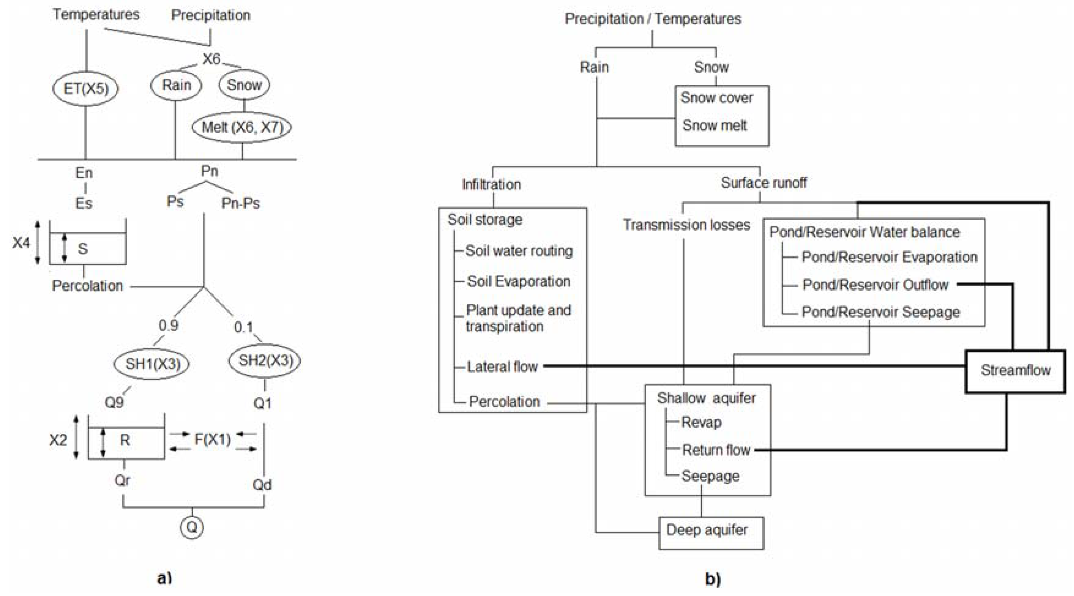
3.1. GR4J and SWAT Model Descriptions
3.2. Low-Flow Indices
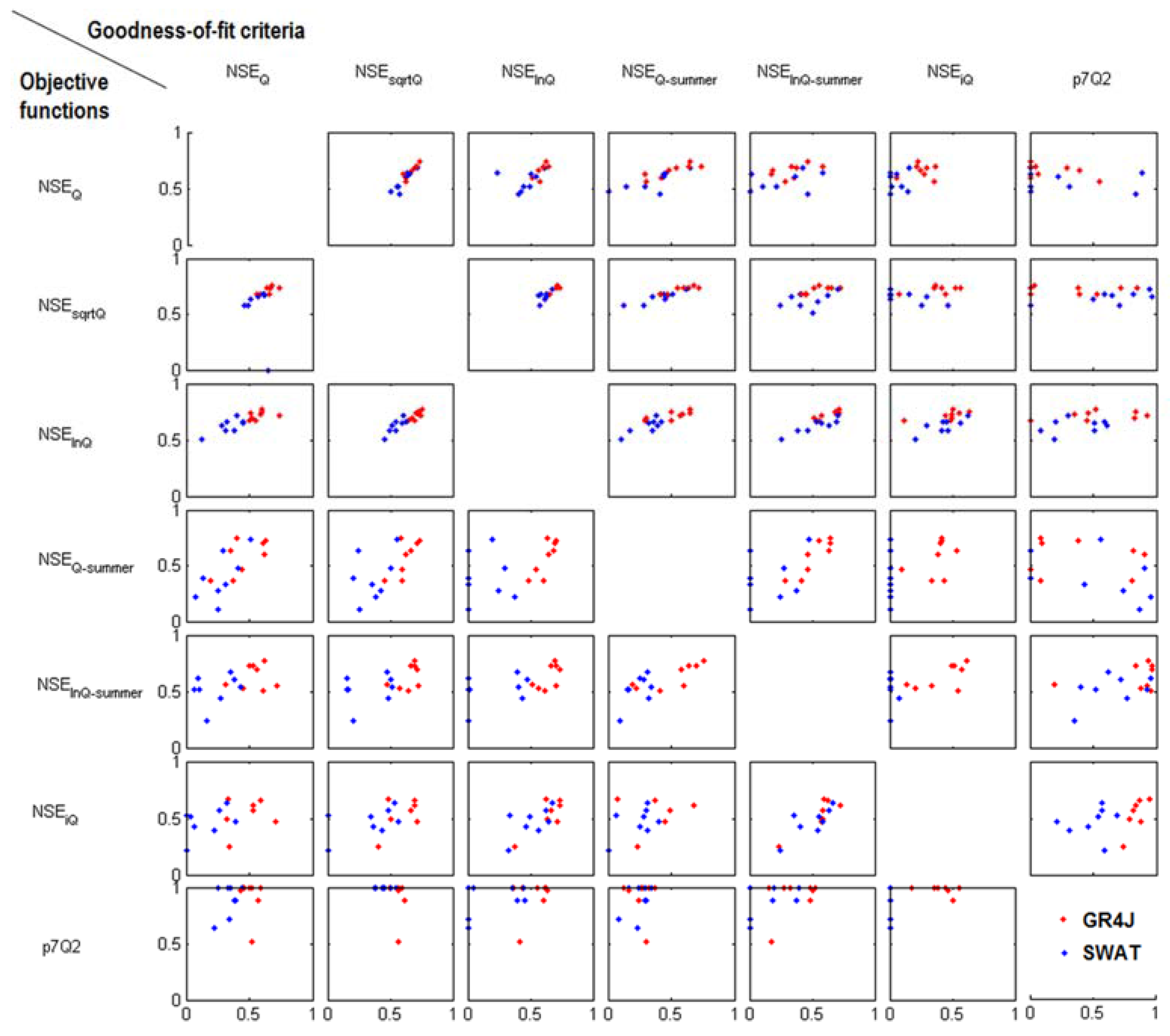
3.3. Calibration, Validation and Statistical Tests
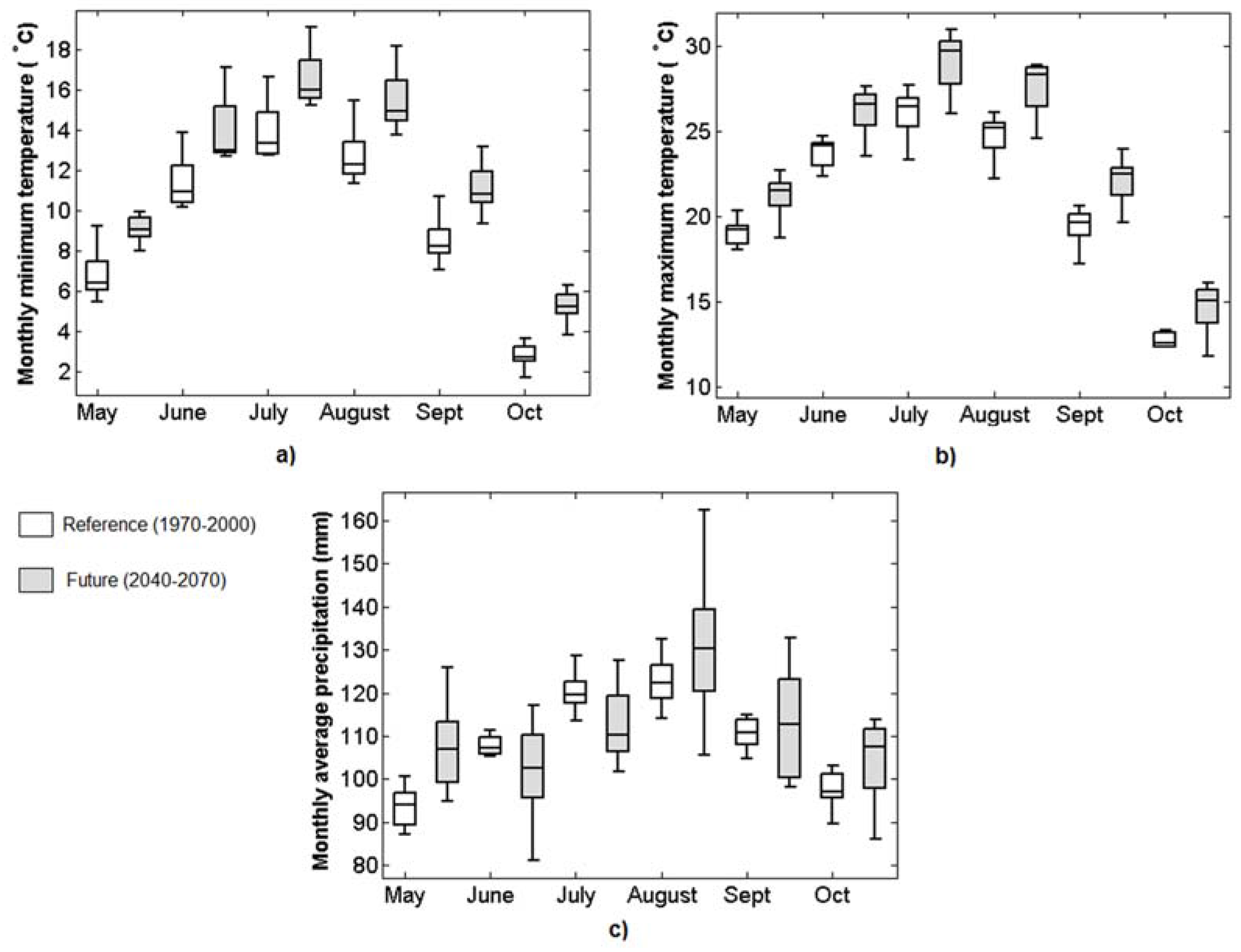
3.4. Climate Change Projections
4. Results and Analysis
4.1. Model Calibration and Validation
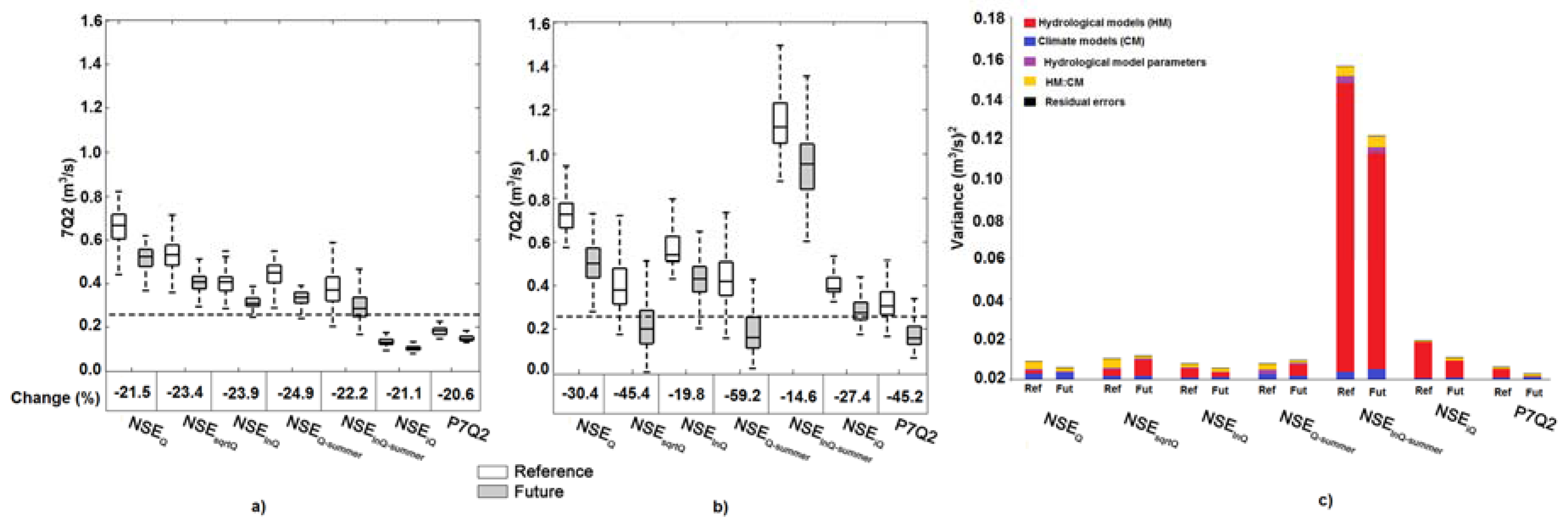
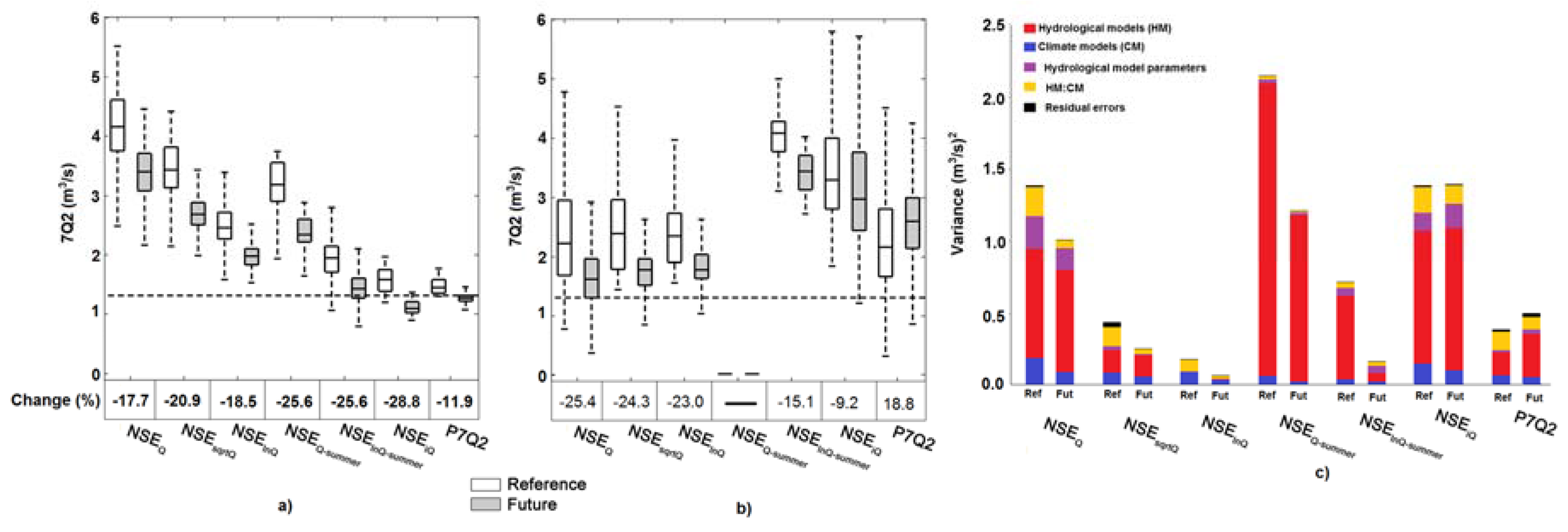
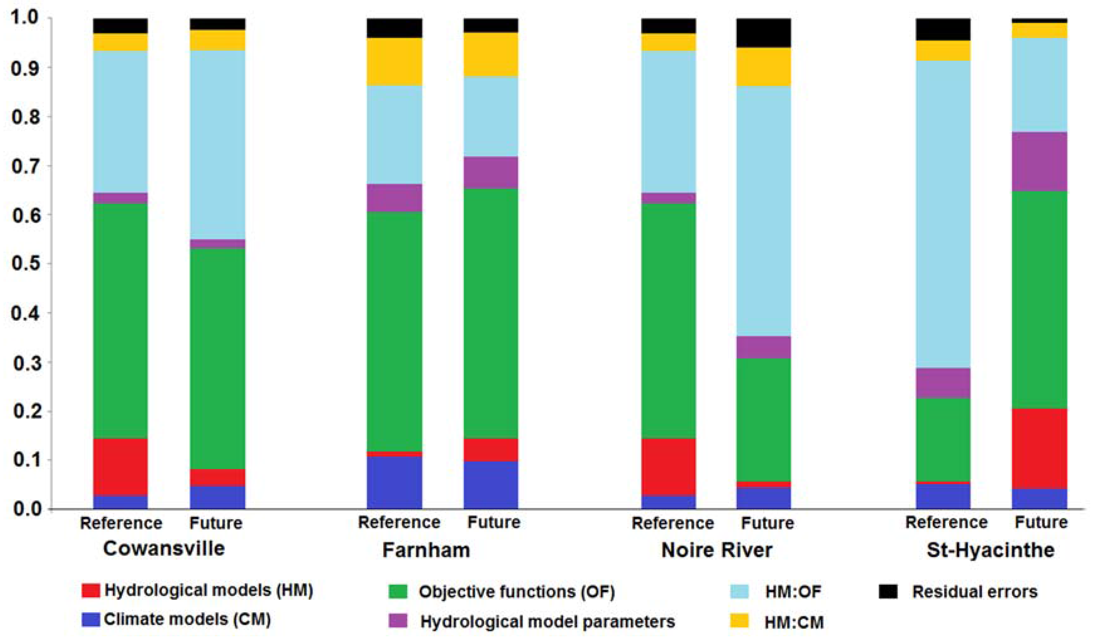
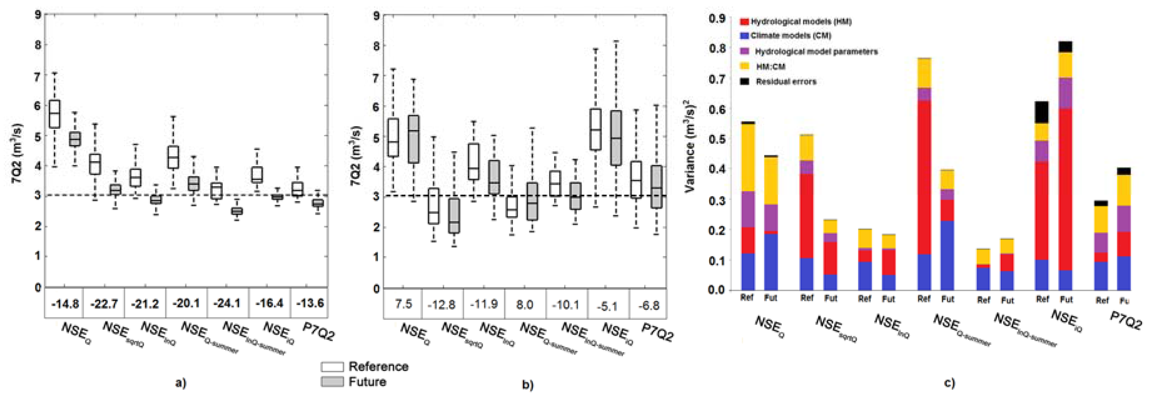
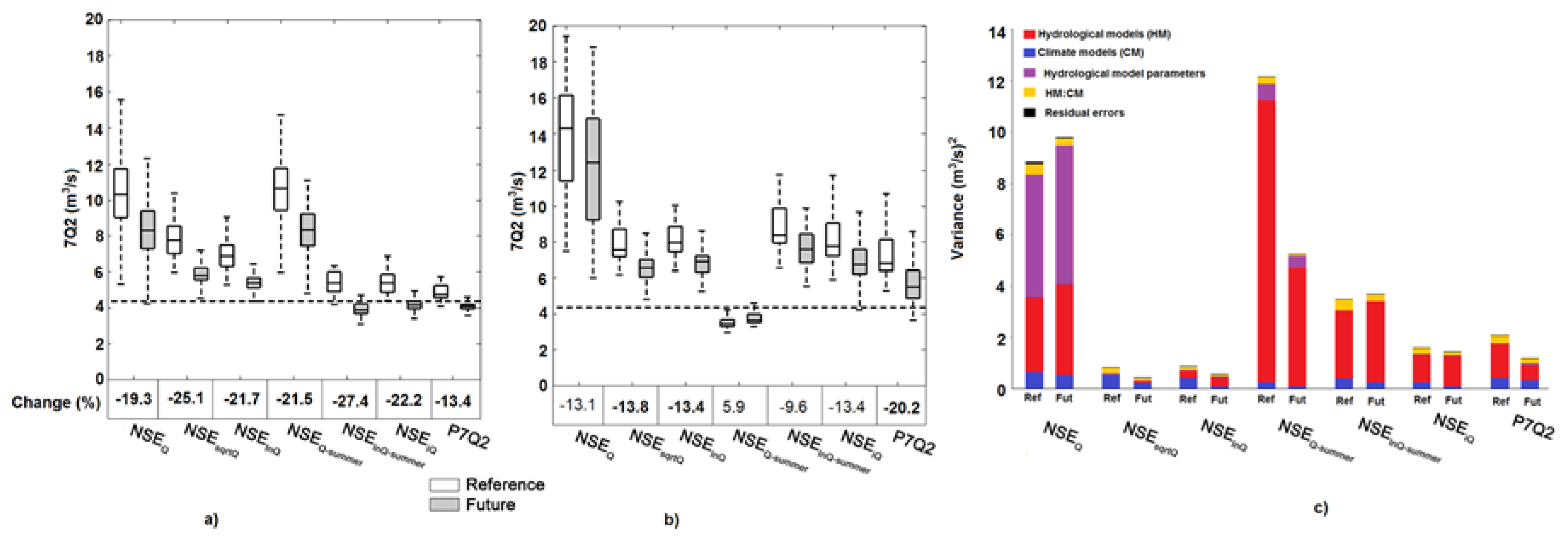
4.2. Future Low-Flow and Uncertainty Analysis
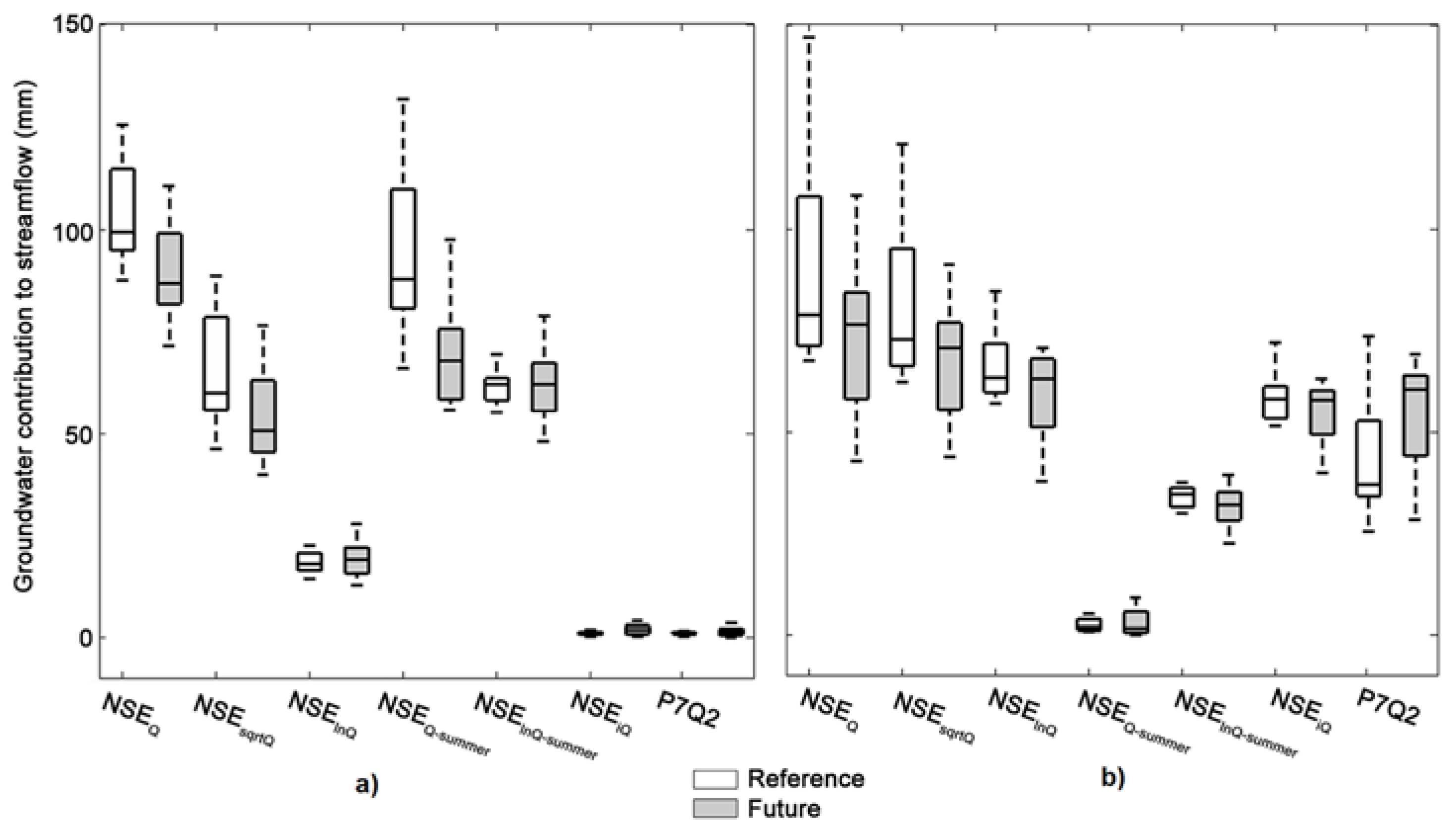
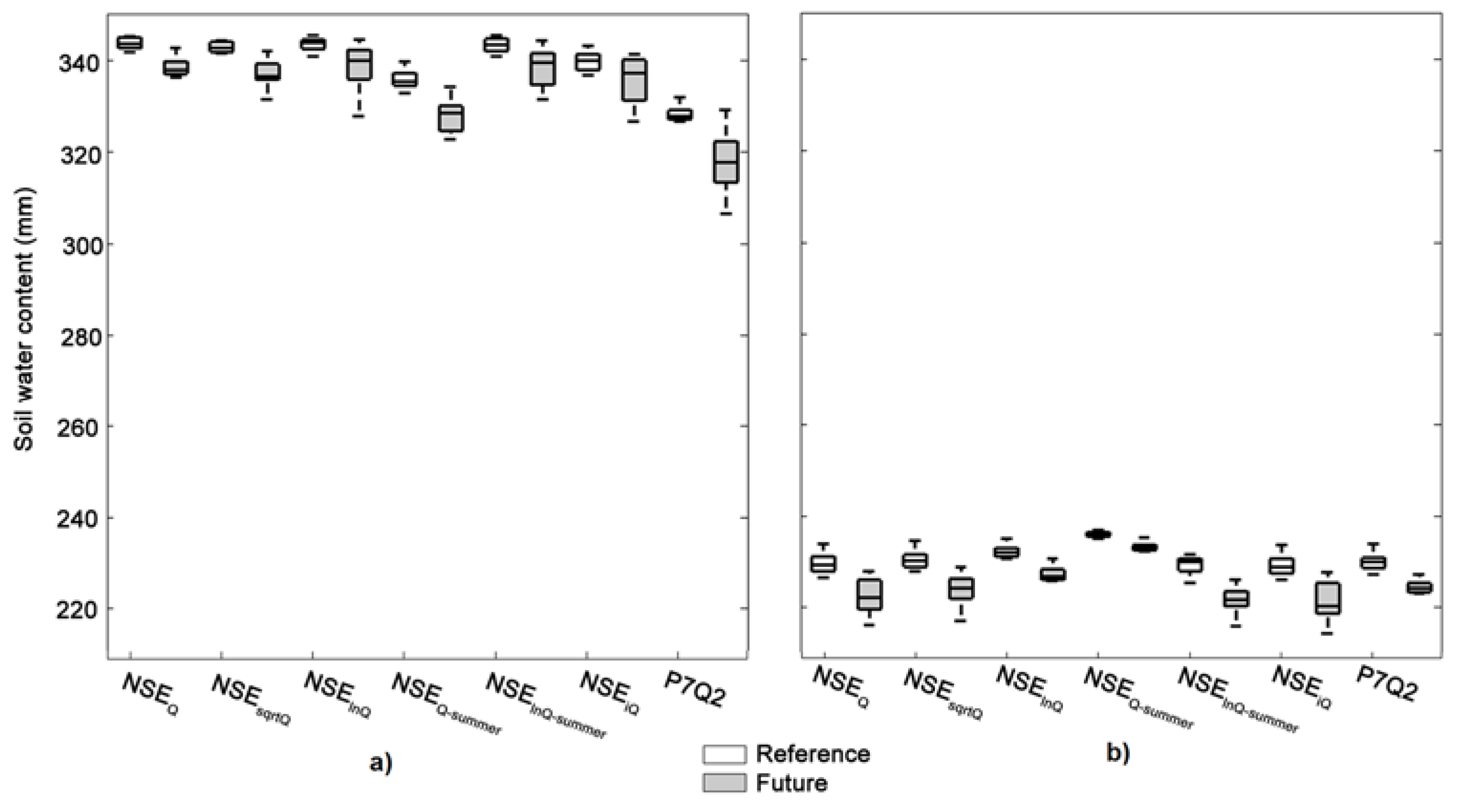
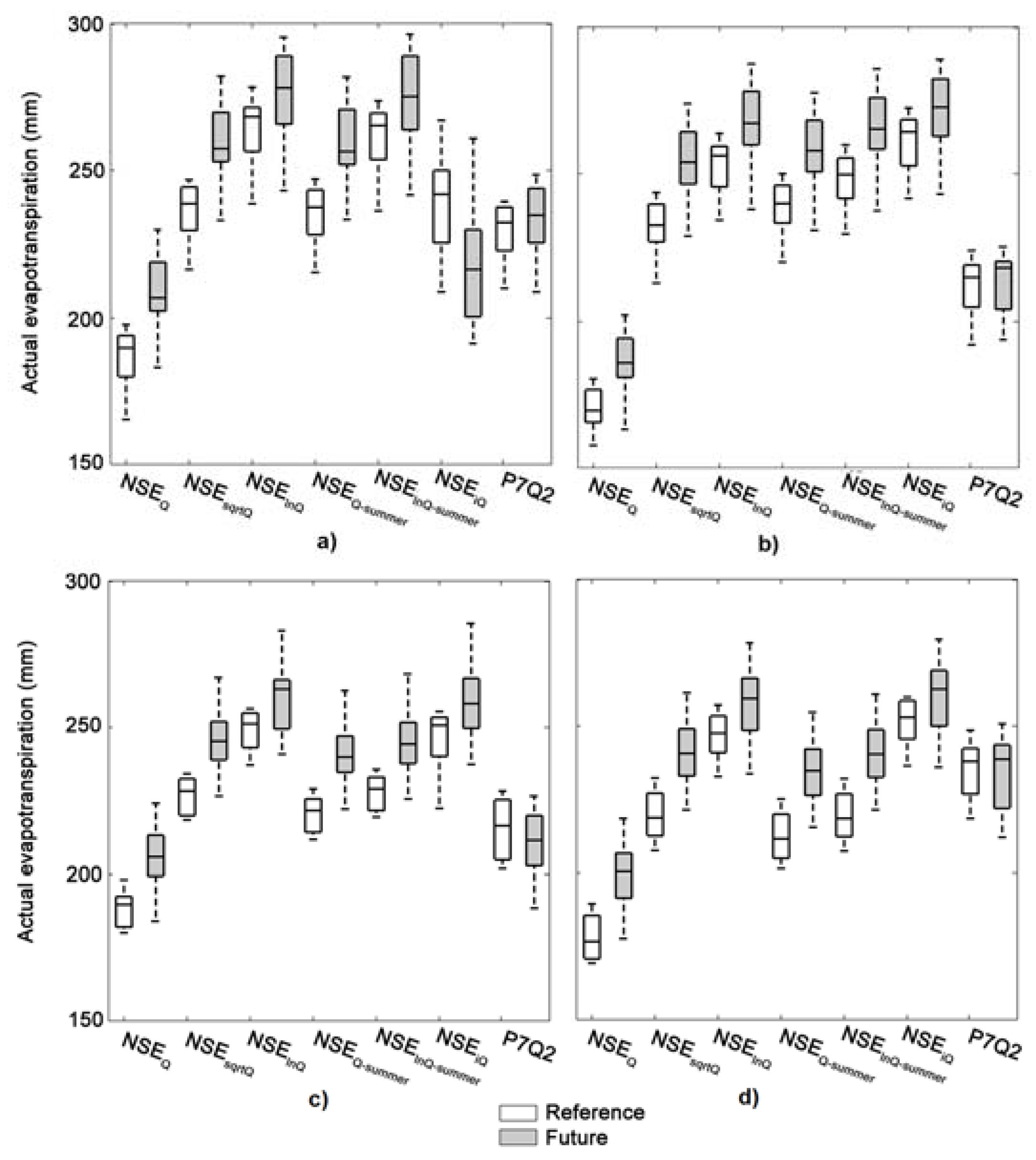
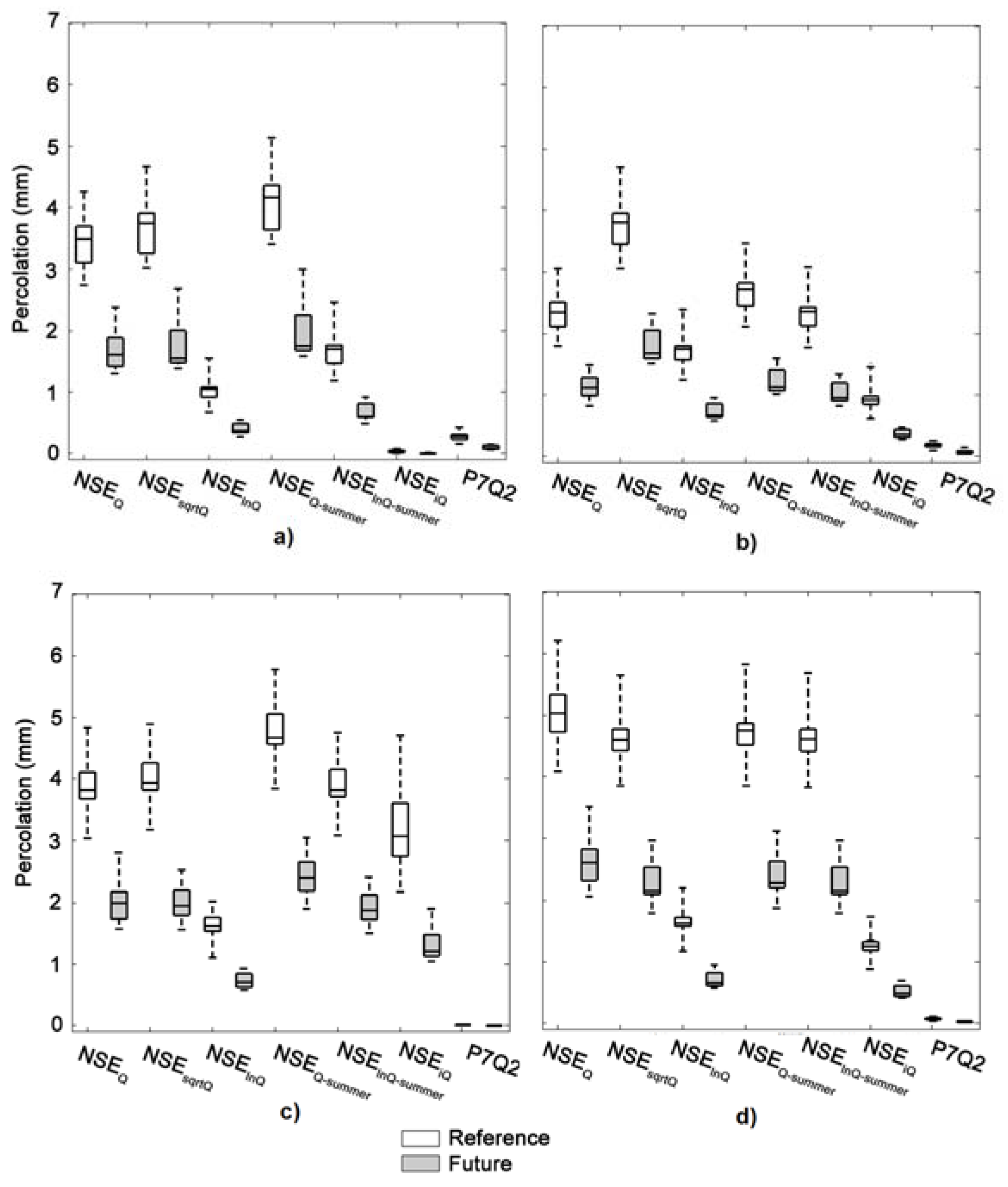
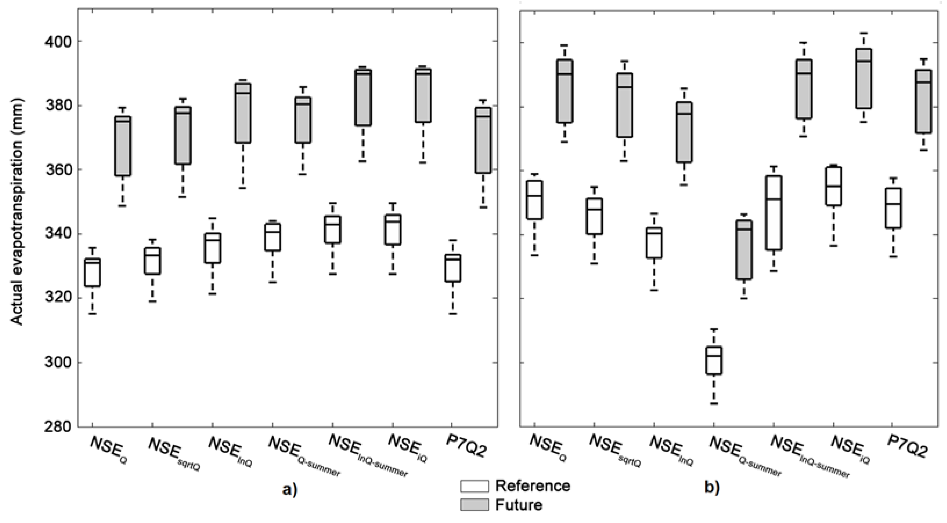
4.3. Hydrological Processes and State Variable Analysis
4.3.1. The GR4J Model
4.3.2. The SWAT Model
5. Discussion and Conclusions
Acknowledgments
Author Contributions
Conflicts of Interest
References
- Mauser, W.; Marke, T.; Stoeber, W. Climate Change and water resources: Scenarios of low-flow conditions in the Upper Danube River Basin. IOP Conf. Ser. Earth Environ. Sci. 2008. [Google Scholar] [CrossRef]
- Rahman, M.; Bolisetti, T.; Balachandar, R. Effect of climate change on low-flow conditions in the Ruscom River Watershed, Ontario. Trans. ASABE 2010, 53, 1521–1532. [Google Scholar] [CrossRef]
- Ryu, J.H.; Lee, J.H.; Jeong, S.; Park, S.K.; Han, K. The impacts of climate change on local hydrology and low flow frequency in the Geum River Basin, Korea. Hydrol. Process. 2011, 25, 3437–3447. [Google Scholar] [CrossRef]
- Centre d’expertise hydrique du Québec (CEHQ). Atlas Hydroclimatique du Québec Méridional—Impact des Changements Climatiques sur les Régimes de Crue, D’étiage et D’hydraulicité à L’horizon 2050; Centre D’expertise Hydrique du Québec (CEHQ): Ville de Québec, QC, Canada, 2015; p. 81. [Google Scholar]
- Wilby, R.L.; Harris, I. A framework for assessing uncertainties in climate change impacts: Low-flow scenarios for the River Thames, UK. Water Resour. Res. 2006, 42, W02419. [Google Scholar] [CrossRef]
- Kay, A.L.; Davies, H.N.; Bell, V.A.; Jones, R.G. Comparison of uncertainty sources for climate change impacts: Flood frequency in England. Clim. Chang. 2009, 92, 41–63. [Google Scholar] [CrossRef] [Green Version]
- Chen, J.; Brissette, F.P.; Leconte, R. Uncertainty of downscaling method in quantifying the impact of climate change on hydrology. J. Hydrol. 2011, 401, 190–202. [Google Scholar] [CrossRef]
- Bosshard, T.; Carambia, M.; Goergen, K.; Kotlarski, S.; Krahe, P.; Zappa, M.; Schär, C. Quantifying uncertainty sources in an ensemble of hydrological climate-impact projections. Water Resour. Res. 2013, 49, 1523–1536. [Google Scholar] [CrossRef]
- Andor, N.; Rössler, O.; Köplin, N.; Huss, M.; Weingartner, R.; Seibert, J. Robust changes and sources of uncertainty in the projected hydrological regimes of Swiss Catchments. Water Resour. Res. 2014, 50, 7541–7562. [Google Scholar]
- Najafi, M.R.; Moradkhani, H.; Jung, I.W. Assessing the uncertainties of hydrologic model selection in climate change impact studies. Hydrol. Process. 2011, 25, 2814–2826. [Google Scholar] [CrossRef]
- Velàzquez, J.A.; Schmid, J.; Ricard, S.; Muerth, M.J.; Gauvin St-Denis, B.; Minville, M.; Chaumont, D.; Caya, D.; Ludwig, R.; Turcotte, R. An ensemble approach to assess hydrological models’ contribution to uncertainties in the analysis of climate change impact on water resources. Hydrol. Earth Syst. Sci. 2013, 17, 565–578. [Google Scholar] [CrossRef]
- Vansteenkiste, T.; Tavakoli, M.; Ntegeka, V.; de Smedt, F.; Batelaan, O.; Pereira, F.; Willems, P. Intercomparison of hydrological model structures and calibration approaches in climate scenario impact projections. J. Hydrol. 2014, 519, 743–755. [Google Scholar] [CrossRef]
- Dams, J.; Nossent, J.; Senbeta, T.B.; Willems, P.; Batelaan, O. Multi-model approach to assess the impact of climate change on runoff. J. Hydrol. 2015, 529, 1601–1616. [Google Scholar] [CrossRef]
- Parajka, J.; Blaschke, A.P.; Blöschl, G.; Haslinger, K.; Hepp, G.; Laaha, G.; Schöner, W.; Trautvetter, H.; Viglione, A.; Zessner, M. Uncertainty contributions to low-flow projections in Austria. Hydrol. Earth Syst. Sci. 2016, 20, 2085–2101. [Google Scholar] [CrossRef]
- Beven, K. A manifesto for the equifinality thesis. J. Hydrol. 2006, 320, 18–36. [Google Scholar] [CrossRef] [Green Version]
- Her, Y.; Chaubey, I. Impact of the numbers of observations and calibration parameters on equifinality, model performance, and output and parameter uncertainty. Hydrol. Process. 2015, 29, 4220–4237. [Google Scholar] [CrossRef]
- Yang, J.; Reichert, P.; Abbaspour, K.C.; Xia, J.; Yang, H. Comparing uncertainty analysis techniques for a SWAT application to the Chaohe Basin in China. J. Hydrol. 2008, 358, 1–23. [Google Scholar] [CrossRef]
- Zhang, J.; Li, Q.; Guo, B.; Gong, H. The comparative study of multi-site uncertainty evaluation method based on SWAT model. Hydrol. Process. 2015, 29, 2994–3009. [Google Scholar] [CrossRef]
- Vrugt, J.A.; Gupta, H.V.; Bouten, W.; Sorooshian, S. A shuffled complex evolution metropolis algorithm for optimization and uncertainty assessment of hydrologic model parameters. Water Resour. Res. 2003. [Google Scholar] [CrossRef]
- Beven, K.; Binley, A. The future of distributed models: Model calibration and uncertainty prediction. Hydrol. Process. 1992, 6, 279–298. [Google Scholar] [CrossRef]
- Beven, K.; Binley, A. GLUE: 20 years on. Hydrol. Process. 2014, 28, 5897–5918. [Google Scholar] [CrossRef]
- Abbaspour, K.C.; Yang, J.; Maximov, I.; Siber, R.; Bogner, K.; Mieleitner, J.; Zobrist, J.; Srinivasan, R. Spatially-distributed modelling of hydrology and water quality in the pre-alpine/alpine Thur watershed using SWAT. J. Hydrol. 2007, 333, 413–430. [Google Scholar] [CrossRef]
- Van Griensven, A.; Meixner, T. A global and efficient multi-objective auto-calibration and uncertainty estimation method for water quality catchment models. J. Hydroinform. 2007, 9, 277–291. [Google Scholar] [CrossRef]
- Nash, J.E.; Sutcliffe, J.V. River flow forecasting through conceptual models part I—A discussion of principles. J. Hydrol. 1970, 10, 282–290. [Google Scholar] [CrossRef]
- OBV Yamaska. Plan directeur de L’eau, 2e Version; Organisme de Basin Versant de la Yamaska: Granby, QC, Canada, 2014. [Google Scholar]
- Perrin, C.; Michel, C.; Andréassian, V. Improvement of a parsimonious model for streamflow simulation. J. Hydrol. 2003, 279, 275–289. [Google Scholar] [CrossRef]
- Hamon, W.R. Estimating potential evapotranspiration. J. Hydraul. Eng. Div. 1961, 87, 107–120. [Google Scholar]
- Arnold, J.G.; Srinivasan, R.; Muttiah, R.S.; Williams, J.R. Large area hydrologic modeling and assessment Part I: Model development. J. Am. Water Resour. Assoc. 1998, 34, 73–89. [Google Scholar] [CrossRef]
- Neitsch, S.L.; Arnold, J.G.; Kiniry, J.R.; Williams, J.R. Soil and Water Assessment Tool Theoretical Documentation Version 2009; Grassland, Soil and Water Research Laboratory, Agricultural ResearchService and Blackland Research Center, Texas Agricultural Experiment Station: College Station, TX, USA, 2011. [Google Scholar]
- Ministère de développement durable, de l’environnement et des parcs (MDDEP). Calcul et Interprétation des Objectifs Environnementaux de Rejet Pour les Contaminants du Milieu Aquatique, 2nd ed.; Direction du Suivi de L’état de L’environnement; Québec, Ministère du Développement Durable, de L’environnement et des Parcs: Rimouski, QC, Canada, 2007; p. 56. [Google Scholar]
- Ministère du Développement Durable, de L’environnement et de la Lutte Contre les Changements Climatiques (MDDELCC). Guide de Production des Installations de Production d’eau Potable; Ministère du Développement Durable, de L’environnement et de la Lutte Contre les Changements Climatiques: Rimouski, QC, Canada, 2015. [Google Scholar]
- Duan, Q.; Sorooshian, S.; Gupta, V. Effective and efficient global optimization for conceptual rainfall-runoff models. Water Resour. Res. 1992, 28, 1015–1031. [Google Scholar] [CrossRef]
- Ritter, A.; Munoz-Carpena, R. Performance evaluation of hydrological models: Statistical significance for reducing subjectivity in goodness-of-fit assessments. J. Hydrol. 2013, 480, 33–45. [Google Scholar] [CrossRef]
- McCuen, R.H.; Knight, Z.; Cutter, A.G. Evaluation of the Nash-Sutcliffe Efficiency Index. J. Hydrol. Eng. 2006, 11, 597–602. [Google Scholar] [CrossRef]
- Gupta, H.V.; Kling, H. On typical range, sensitivity, and normalization of Mean Squared Error and Nash-Sutcliffe Efficiency type metrics. Water Resour. Res. 2011, 47, 1–3. [Google Scholar] [CrossRef]
- Pushpalatha, R.; Perrin, C.; Le Moine, N.; Andréassian, V. A review of efficiency criteria suitable for evaluating low-flow simulations. J. Hydrol. 2012, 420, 171–182. [Google Scholar] [CrossRef]
- Mearns, L.; McGinnin, S.; Arritt, R.; Biner, S.; Duffy, P.; Gutowski, W.; Isaac, H.; Richard, J.; Leung, R.; Nunes, A.; et al. The North American Regional Climate Change Assessment Program Dataset; National Center for Atmospheric Research Earth System Grid Data Portal: Boulder, CO, USA, 2007. [Google Scholar]
- Caya, D.; Laprise, R. A semi-implicit semi-lagrangian regional climate model: The Canadian RCM. Mon. Weather Rev. 1999, 127, 341–362. [Google Scholar] [CrossRef]
- Flato, G. The Third Generation Coupled Global Climate Model (CGCM3). Available online: http://www.ec.gc.ca/ccmac-cccma/default.asp?n=1299529F-1 (accessed on 28 February 2017).
- Schmidli, L.; Frei, C.; Vidal, P. Downscaling from GCM precipitation: A benchmark for dynamical and statistical downscaling methods. Int. J. Climatol. 2006, 26, 679–686. [Google Scholar] [CrossRef]
- Ouranos. Vers L’adaptation. Synthèse des Connaissances sur les Changements Climatiques au Québec. Partie 1: Évolution Climatique au Québec; Ouranos: Montréal, QC, Canada, 2015. [Google Scholar]


| Sub-Watershed | Drainage Area (km2) | Slope (%) | Land Cover—Forest (%) | Land Cover—Crops (%) |
|---|---|---|---|---|
| Cowansville | 214 | 8.42 | 73.0 | 19.6 |
| Farnham | 1202 | 5.42 | 51.6 | 33.6 |
| Noire River | 1414 | 2.77 | 40.7 | 53.2 |
| St-Hyacinthe | 3289 | 3.49 | 43.2 | 52.1 |
| Goodness-of-Fit (Group) | Description | Equation |
|---|---|---|
| NSEQ (1) | NSE calculated on streamflows | |
| NSEsqrtQ (2) | NSE calculated on root squared transformed streamflows | |
| NSElnQ (2) | NSE calculated on log-transformed streamflows | |
| NSEQ-summer (3) | NSE calculated on streamflows between May and October | |
| NSElnQ-summer (3) | NSE calculated on log transformed streamflows between May and October | |
| NSEiQ (4) | NSE calculated on inverse transformed streamflows | |
| NSEQ and p7Q2 (4) | The 7-day low-flow value with a 2-year return period combined with a threshold on NSE calculated on streamflows | and |
| Level of S (%)—Period | NSEQ | NSEsqrtQ | NSElnQ | NSEQ-summer | NSElnQ-summer | NSEiQ | P7Q2 |
|---|---|---|---|---|---|---|---|
| Cowansville | |||||||
| Maximum—reference | 90.8 | 87.0 | 86.2 | 86.0 | 87.3 | 89.3 | 89.0 |
| Minimum—reference | 52.2 | 46.8 | 32.8 | 47.9 | 37.6 | 12.4 | 26.4 |
| Maximum—future | 91.6 | 88.4 | 87.8 | 87.2 | 86.1 | 90.8 | 90.6 |
| Minimum—future | 37.3 | 32.2 | 19.9 | 33.2 | 23.7 | 6.5 | 16.2 |
| Farnham | |||||||
| Maximum—reference | 92.2 | 86.5 | 85.9 | 86.4 | 85.9 | 85.7 | 90.3 |
| Minimum—reference | 50.5 | 46.6 | 38.1 | 43.5 | 41.2 | 31.9 | 24.3 |
| Maximum—future | 92.7 | 87.8 | 87.5 | 87.7 | 87.4 | 87.4 | 91.6 |
| Minimum—future | 36.1 | 32.9 | 24.8 | 29.3 | 27.1 | 19.6 | 15.0 |
| Noire River | |||||||
| Maximum—reference | 89.1 | 85.6 | 84.3 | 85.7 | 85.7 | 85.3 | 85.1 |
| Minimum—reference | 51.7 | 46.8 | 36.7 | 49.1 | 46.7 | 41.7 | 10.8 |
| Maximum—future | 90.2 | 86.6 | 85.6 | 86.9 | 86.3 | 86.5 | 87.3 |
| Minimum—future | 38.0 | 33.3 | 23.8 | 35.7 | 33.3 | 27.7 | 6.0 |
| St-Hyacinthe | |||||||
| Maximum—reference | 89.8 | 86.8 | 85.3 | 87.0 | 87.0 | 85.4 | 86.6 |
| Minimum—reference | 56.0 | 49.4 | 37.3 | 50.6 | 49.4 | 34.5 | 17.8 |
| Maximum—future | 90.7 | 87.9 | 86.7 | 88.3 | 88.3 | 86.9 | 88.4 |
| Minimum—future | 41.4 | 35.4 | 23.6 | 36.4 | 35.4 | 21.6 | 10.0 |
| Level of R (%)—Period | NSEQ | NSEsqrtQ | NSElnQ | NSEQ-summer | NSElnQ-summer | NSEiQ | P7Q2 |
|---|---|---|---|---|---|---|---|
| Cowansville | |||||||
| Maximum—reference | 68.4 | 71.1 | 70.4 | 74.3 | 77.9 | 78.6 | 68.4 |
| Minimum—reference | 52.1 | 50.8 | 46.0 | 55.6 | 48.4 | 49.0 | 44.5 |
| Maximum—future | 69.4 | 71.7 | 71.0 | 76.0 | 73.3 | 81.4 | 69.9 |
| Minimum—future | 47.6 | 46.4 | 43.0 | 50.3 | 44.4 | 46.1 | 41.6 |
| Farnham | |||||||
| Maximum—reference | 57.9 | 63.3 | 63.8 | 68.8 | 67.7 | 59.5 | 58.3 |
| Minimum—reference | 45.1 | 45.4 | 43.8 | 49.8 | 47.0 | 40.0 | 40.5 |
| Maximum—future | 58.5 | 63.7 | 64.1 | 69.3 | 68.1 | 60.0 | 58.6 |
| Minimum—future | 42.8 | 42.0 | 40.7 | 46.2 | 43.4 | 37.7 | 38.7 |
| Noire River | |||||||
| Maximum—reference | 64.6 | 68.8 | 71.6 | 75.2 | 79.1 | 89.1 | 63.1 |
| Minimum—reference | 49.0 | 49.7 | 49.2 | 54.6 | 54.2 | 57.9 | 38.2 |
| Maximum—future | 65.2 | 70.0 | 73.1 | 76.7 | 77.9 | 87.2 | 63.2 |
| Minimum—future | 45.1 | 45.4 | 45.2 | 49.3 | 48.8 | 52.2 | 36.5 |
| St-Hyacinthe | |||||||
| Maximum—reference | 63.7 | 67.0 | 67.0 | 64.8 | 73.2 | 71.3 | 63.9 |
| Minimum—reference | 48.3 | 47.7 | 45.2 | 48.7 | 51.2 | 47.0 | 39.3 |
| Maximum—future | 64.0 | 66.9 | 67.3 | 65.2 | 73.5 | 72.0 | 63.3 |
| Minimum—future | 44.4 | 43.4 | 41.6 | 44.6 | 46.1 | 43.2 | 37.2 |
© 2017 by the authors. Licensee MDPI, Basel, Switzerland. This article is an open access article distributed under the terms and conditions of the Creative Commons Attribution (CC BY) license ( http://creativecommons.org/licenses/by/4.0/).
Share and Cite
Trudel, M.; Doucet-Généreux, P.-L.; Leconte, R. Assessing River Low-Flow Uncertainties Related to Hydrological Model Calibration and Structure under Climate Change Conditions. Climate 2017, 5, 19. https://doi.org/10.3390/cli5010019
Trudel M, Doucet-Généreux P-L, Leconte R. Assessing River Low-Flow Uncertainties Related to Hydrological Model Calibration and Structure under Climate Change Conditions. Climate. 2017; 5(1):19. https://doi.org/10.3390/cli5010019
Chicago/Turabian StyleTrudel, Mélanie, Pierre-Louis Doucet-Généreux, and Robert Leconte. 2017. "Assessing River Low-Flow Uncertainties Related to Hydrological Model Calibration and Structure under Climate Change Conditions" Climate 5, no. 1: 19. https://doi.org/10.3390/cli5010019