
Climatic Study of the Marine Surface Wind Field over the Greek Seas with the Use of a High Resolution RCM Focusing on Extreme Winds


1
Institute of Meteorology, Freie Universität Berlin, Berlin 14195, Germany
2
Department of Meteorology and Climatology, School of Geology, Faculty of Sciences, Aristotle University of Thessaloniki, Thessaloniki 54124, Greece
*
Author to whom correspondence should be addressed.
Climate 2017, 5(2), 29; https://doi.org/10.3390/cli5020029
Submission received: 22 February 2017
/
Revised: 20 March 2017
/
Accepted: 25 March 2017
/
Published: 31 March 2017
(This article belongs to the Special Issue Climate Extremes, the Past and the Future)
Abstract
:The marine surface wind field (10 m) over the Greek seas is analyzed in this study using The RegCM. The model’s spatial resolution is dynamically downscaled to 10 km × 10 km, in order to simulate more efficiently the complex coastlines and the numerous islands of Greece. Wind data for the 1980–2000 and 2080–2100 periods are produced and evaluated against real observational data from 15 island and coastal meteorological stations in order to assess the model’s ability to reproduce the main characteristics of the surface wind fields. RegCM model shows a higher simulating skill to project seasonal wind speeds and direction during summer and the lowest simulating skill in the cold period of the year. Extreme wind speed thresholds were estimated using percentiles indices and three Peak Over Threshold (POT) techniques. The mean threshold values of the three POT methods are used to examine the inter-annual distribution of extreme winds in the study region. The highest thresholds were observed in three poles; the northeast, the southeast, and the southwest of Aegean Sea. Future changes in extreme speeds show a general increase in the Aegean Sea, while lower thresholds are expected in the Ionian Sea. Return levels for periods of 20, 50, 100, and 200 years are estimated.
1. Introduction
Knowledge of the spatial variability of the marine wind field is important, since it induces heat and momentum transfers between the ocean and the atmosphere [1]. Furthermore, it has important consequences in the ocean circulation, both permanent and transient, such as in considering the dense water formation and the ocean upwelling, for instance [2]. In the Intergovernmental Panel on Climate Change’s (IPCC) special report for extreme events [3] is stated that extreme wind speeds pose a threat to human safety, maritime and aviation activities, and the integrity of infrastructure. As well as extreme wind speeds, other attributes of wind can cause extreme impacts. Trends in average wind speed can influence potential evaporation and in turn water availability and droughts [4]. Sustained mid-latitude winds can elevate coastal sea levels [5], while longer-term changes in prevailing wind direction can cause changes in wave climate and coastline stability [6].
As a weather and climate variable, surface wind can be described as “complicated” due to its two major characteristics. Its vector form, for which a pair of values is required (horizontal components u and v, or speed and direction), and its intense variability, both in space and time. Over the oceans and major seas the effect of topography and land friction on the spatial wind variability diminishes, resulting in a smoother wind field. In contrast, over smaller seas, coastal regions with complex coastlines, and seas containing islands, the surface wind field can become more inconsistent. In such areas, the use of dynamically downscaled, high resolution Regional Climate Models (RCMs) have been shown to produce more realistic results of the wind flow, when compared to coarser General Circulation Models (GCMs) or reanalysis products [7,8].
The Mediterranean Sea is characterized by its semi-closed status and the large extent of steep coastlines, due to the numerous mountain chains surrounding it. As stated by Zecchetto and De Biasio [9], the complexity of the coastal orography and the presence of mountainous islands deeply influence the local-scale atmospheric circulation in the Ekman layer, producing local effects at spatial scales down to a few kilometers. The region of interest of this study is the Greek seas. Two are the main seas in Greece, the Aegean and the Ionian, covering the areas east and west of the Greek mainland, respectively. They include both complex coastlines and numerous islands. Consequently, it is reasonable to expect that under these regional characteristics the application of a high-resolution RCM would be of most value in the study of maritime surface wind.
The IPCC [10] assessment report states that evidence of model skill in simulation of wind extremes is mixed. However, this refers mostly to surface wind over land. Weisse [11] found that the REMO RCM, forced by the NCEP–NCAR reanalysis, simulated a very realistic wind climate over the North Sea, including the number and intensity of storms. Most PRUDENCE RCMs (http://prudence.dmi.dk/), while quite realistic over sea, severely underestimate the occurrence of very high wind speeds over land and coastal areas [12].
Studies about the extreme winds in Europe, using RCMs, are mainly focused in its central and northern regions [13,14,15]. A very comprehensive assessment of the ability of a 12 RCM ensemble to simulate the surface wind field over the Mediterranean region was performed through the collaborative project CLIM-RUN [16]. Most of the RCMs had a spatial resolution of 25 km, and for future projections considered the SRES A1B climate scenario. For the future projections of extreme winds the IPCC SREX states that there is generally low confidence because of the relatively few studies and shortcomings in the simulation of these events. Walshaw [17] found that annual wind extremes for coastal locations will typically be highest at mid-latitudes.
Extreme values as all statistical values can be estimated either by non-parametric statistics, such as percentile indices, or by parametric methods based on the extreme value theory (EVT) [18]. According to the EVT, there are two main approaches for estimating extreme values. In the first and oldest one, called ‘Block Maxima’, the data are divided in blocks with each containing an equal number of values. Then, the maximum value of each block is extracted to form a new data set to which the Generalized Extreme Value (GEV) distribution is applied. The main drawback of this method is the limited number of values (maxima), especially in short time series. The evolution of the EVT led to the second approach, called Peaks Over Threshold (POT), where a threshold value is selected and then the asymptotic Generalized Pareto Distribution (GPD) is applied to describe the set of values which exceed this threshold. The key aspect in this approach is the appropriate threshold selection. In this study, both POT methods and percentile indices are applied, based on the study by Anagnostopoulou and Tolika [19], for estimating extreme precipitation values over Europe. In order to deal with the sensitive concept of the POT’s threshold selection, three POT methods are applied: the Mean Residual Life (MRL), the Threshold Choice (TC), and the Dispersion Index (DI), and the mean of their resulting threshold is chosen as the final threshold.
The two main objectives of the present study are: (i) to evaluate the ability of the RegCM3 in capturing the main characteristics of the marine wind field around Greece; and (ii) to perform a reliable application of Peaks Over Threshold techniques in order to estimate extreme wind speed thresholds and return levels. Therefore, this study makes a major contribution to research on climatological characteristics of extreme winds over the eastern Mediterranean region by demonstrating, for the first time, high resolution simulations of wind.
2. Materials and Methods
2.1. Materials
The model employed for this study is the third generation of the RegCM regional climate model, originally developed at the National Center for Atmospheric Research (NCAR). It is supported by the Abdus Salam International Centre for Theoretical Physics (ICTP) in Trieste, Italy. RegCM3 is a 3-dimensional, hydrostatic, compressible, sigma coordinate, primitive equation RCM. Initially, the model runs for a large window, from 30 N to 50 N and from 10 W to 40 E, with a horizontal grid resolution of 25 km. Then, the model was nested inside this window, with a horizontal resolution of 10 km, covering the area from 18.5° E to 29.5° E and from 34.5° N to 42° N. For both resolutions, the model has 18 vertical σ-levels. The driving global data used come from the ECHAM5 GCM, and the SRES A1B emission scenario for future climate projections is used.
The Massachusetts Institute of Technology–Emanuel scheme [20,21] is the chosen cumulus convective scheme of the model [22]. The Subgrid Explicit Moisture Scheme (SUBEX) is used for the Large-Scale Precipitation Scheme. The Biosphere–Atmosphere Transfer Scheme (BATS) is used to parameterize the land-surface interactions. For the model run with 10 km horizontal resolution, some of the parameters in the precipitation parameterization are adjusted, according to Thomas et al. [23].
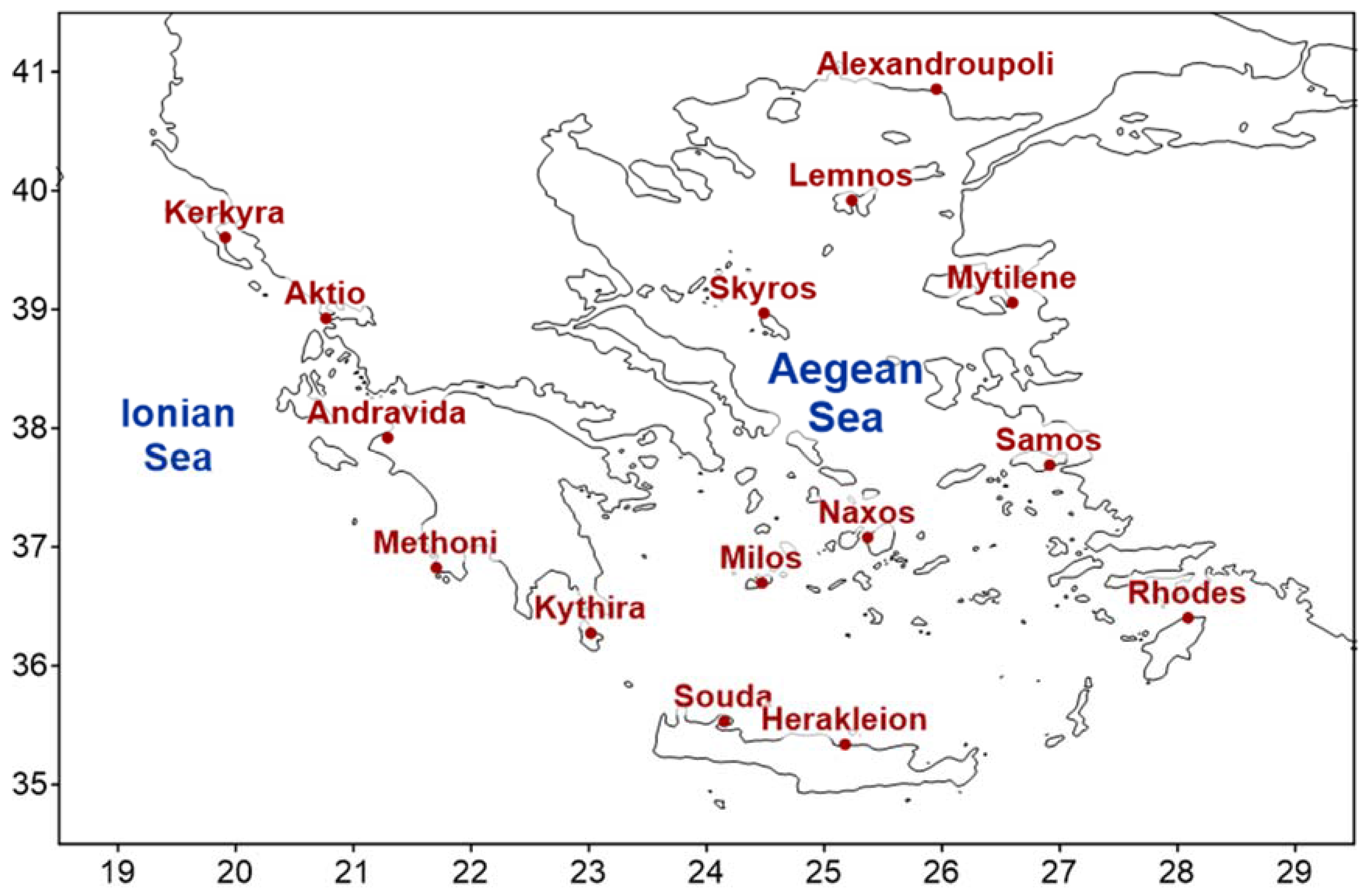
The model’s data consist of mean daily wind speed (m/s) and mean daily wind direction (degrees) at 10 m height above sea surface (or land). They correspond to the control period, 1980–2000, and to the future projection for the period 2080–2100. Also, similar observation data from 15 coastal and island meteorological stations are used for the evaluation of the RegCM3’s simulation (Figure 1).
2.2. Methods
The initial aim of this study is to evaluate the seasonal results obtained from the RegCM3 against those from the observation data, for the control period (1980–2000). This evaluation process consists of two steps.
In the first step, Principal Component Analysis (PCA) is applied to the two datasets, in order to distinguish the existence of regions with similar wind characteristics. After such regions are identified for each dataset, the coincidence of the regions between the two datasets is examined. Different kinds of input data were tested for the PCA, such as wind speed, wind direction, and u and v wind components. The results of the PCAs showed that the combination of the u and v wind components in a single variable is the more appropriate, as it better represents the vector form of wind.
In the second step of the evaluation, direct comparison of a series of wind parameters and statistics is made between the data of the 15 stations and those of the model’s nearest grid points. These include the prevailing wind direction and its frequency, the median wind speed for the prevailing direction, and the median and 95th wind speed percentile accounted for all directions.
After the evaluation, the main wind characteristics are presented. Seasonal maps of mean wind speed and prevailing wind direction are presented for the control period. Also, mean seasonal wind speed differences, accompanied with statistical significance denotations are designed for the future projection. Future differences in prevailing wind directions are almost nonexistent, thus they are not shown.
Next, extreme wind speeds are estimated for the RegCM3’s control and future period data. Three POT methods and three percentile indices are used, and their results are compared. The basis for the POT methods is the use of the asymptotic GPD, which has a shape parameter ξ and a scale parameter σ. For a set of values x the GPD cumulative distribution has the form of:
where u is the chosen threshold and y are the excesses over u, y = x − u. If the GPD is valid for a chosen threshold u0, then it will be also valid for the excesses greater than u [24]. The three POT methods used are: (i) the Mean Residual Life (MRL); (ii) the Threshold Choice (TC); and (iii) the Dispersion Index (DI).
The MRL method [25] is based on the mean of the GPD. It uses the expectation of the GPD excesses E(X − u0 | X > u0) = σuo/(1 − ξ) as a diagnostic, defined for ξ < 1 to ensure that the mean exists. For any higher threshold u > u0 the expectation is
which is linear in u with gradient ξ/(1 − ξ) and intercept σuo/(1 − ξ) [26]. As such, above a threshold u0 at which the GPD provides a valid approximation to the excess distribution the MRL plot should be approximately linear in u [24].
The TC method examines the stability of the GPD parameters when applied for a range of thresholds [27]. Equation (2) results in σu = σuo + ξ (u − u0), so σ depends on u unless ξ = 0. This can be avoided by re-parameterizing the GPD as σ* = σu − ξu which is stable with respect to u. Then, the GPD parameters will exhibit stability for the thresholds u > u0, if u0 is an appropriate threshold.
The DI method is based on the EVT’s acceptance that the excesses over a threshold u0 will follow a Poisson process. If N(t) represents the number of occurrences of an event for time step t, n is the total number of occurrences for the whole period, and λ(t) is the rate of occurrence in t, then the probability of N can be estimated as [28].
The occurrence rate λ refers to independent excesses of u0 for the time t = 1 year. The suitability of the Poisson assumption is tested by the dispersion index [29]
where s2 is the variance of the Poisson process. For suitable thresholds the DI should be close to 1.
As stated by Coles [24], better estimates for return levels are obtained from the appropriate profile likelihood, instead of the delta method, as they are more realistically accounting for the genuine uncertainties of extreme model extrapolation. This can be done by re-parameterizing the equations
where xm is the m-observational return level. The result is
When plotted against the return level period with 95% confidence interval, the profile likelihood gives the lower and upper limits of possible return levels for the given period N years.
The return levels with the lower and upper limit of the profile likelihood for the 95% confidence interval are estimated for 20, 50, 100, and 200 year periods using the Maximum Likelihood Estimation method, based on the models data and extreme values calculated previously.
3. Results
3.1. Evaluation
The results obtained in this study are evaluated against daily surface observations of wind parameters (speed and direction) from meteorological stations of the Hellenic Meteorological Service. The evaluation was made using the nearest (over land) grid point of the model to the stations. Despite the fine horizontal resolution of the model (10 km), some differences between the model and the station data are detected, especially near the coasts and in valleys or small islands due to the model’s inability to reproduce them.
Principal Component Analyses were employed to both data sets (model and observed) for the control period (1980–2000). After applying different tests (see Section 2), it was concluded that the combination of u and v wind components data in a single variable produced the most satisfying results. The explained variance of the first four Principal Components (PCs) accounted for the largest seasonal percentages, with slight differences among the four seasons. For the station data, these percentages varied from 74.4% to 78.5%, and for the model data from 89.6% to 92% (Table 1). The highest percentages are observed for the winter PCA of both data sets. The lowest percentages were found for spring PCA for the station data and for the summer PCA for the model data. The difference in the number of data points between the two datasets should be taken into account in order to explain the 15% difference between the explained variances of their PCAs.
In Figure 2, the results of the winter PCAs for the two datasets are presented, in the form of contours of PC loadings. Four regions are easily distinguished, located in similar areas, both for the model and the observation PCAs. The centers of three of the PCs are located at the edges of the Aegean Sea—the northeastern, the southeastern, and the southwestern part. The center of the fourth PC is found in the Ionian Sea. This pattern can also be detected for the other three seasons (figures not shown), with a gradual increase of the area covering the two south Aegean PCs (hence, the increase of their explained variance percentages) at the expense of the area covering the north Aegean PC.
Moreover, a direct comparison between station and grid point data is conducted for some key wind characteristics. This includes the prevailing wind direction and its mean wind speed; the mean wind speed accounted for all directions and the 95th wind speed percentile, and accounted for all directions too. The seasonal results for the 15 locations are presented in Table 2.
The model is in accordance with the observation data, as far as the wind direction is concerned. As shown in Table 2, the differences in seasonal prevailing wind directions are in the classes of 0° or 45°, almost in every location. Some notable differences are observed in the area of the Ionian Sea.
The RegCM3’s frequencies of the prevailing wind directions seem to be lower than those of the observation data. The most satisfying results are the summer ones, where in 10 out of 15 locations the RegCM3’s percentages deviate between 75% and 125% of the observed prevailing wind direction frequencies. Contrarily, less satisfying results are observed for spring and autumn.
The median wind speeds for the prevailing wind directions of the RegCM3 data are similar to those of the observed data in spring. Diverse results are observed for the other three seasons. For the Ionian Sea, the results can be considered not to be satisfactory for all seasons.
The median wind speed computed for all wind directions shows different seasonal results. In winter and summer the model is in good agreement with the observation data in most parts of the Aegean Sea. In contrast, the areas of southwestern Aegean and the Ionian Sea produce worse results for these two seasons. Higher wind speeds are much better simulated by the RegCM3, as can be seen in the results of the 95th percentile index. There are no deviations outside 50%–150% of the observed values.
It must be noted that there are four locations which (almost) systematically produce unsatisfactory results. Two of them (Alexandroupoli and Andravida) are located on the mainland, and the other two (Souda and Kerkyra), even though they are in island regions, present similarities to the continental terrain.
3.2. Model
3.2.1. Seasonal Variability of Wind Speed and Direction
Figure 3 illustrates the main characteristics of the seasonal surface wind field for the period 1980–2000. In winter, the highest mean seasonal wind speeds (greater than 7 m/s) are detected in (almost) the whole study region, except the northwest of the Aegean Sea. The maximum wind speeds are located in south Greece, where they reach 8.8 m/s. During spring, mean wind speeds rarely exceed 7 m/s, with the areas with the highest values being located south of 37° N (7 m/s–7.5 m/s). The lowest mean speeds occur in the north Aegean Sea. In summer, one of the most constant local wind systems blows over the Aegean Sea, the Etesian winds [30,31]. There is a definite contrast between mean wind speeds in the central and south Aegean Sea and those in the rest of the study region, with the former reaching much higher values. In the southeast Aegean Sea, mean speeds vary between 7 m/s and 10 m/s, while in the north Aegean and west of 23° E mean speeds do not exceed 6 m/s. During autumn, wind speeds increase in the largest part of the domain of interest. The highest values are found in the northeast and the southwest Aegean Sea (8 m/s). In the northwest Aegean Sea, mean speeds do not exceed 7 m/s.
The prevailing wind directions do not vary much throughout the year. The most considerable variations are observed in the Ionian Sea, where the prevailing wintertime western winds gradually shift to northern directions. In the Aegean Sea, northeast winds prevail in the north, north winds prevail in its central part, and northwest winds prevail in its southeast part. Seasonal variations are observed in the south and southwest Aegean Sea.
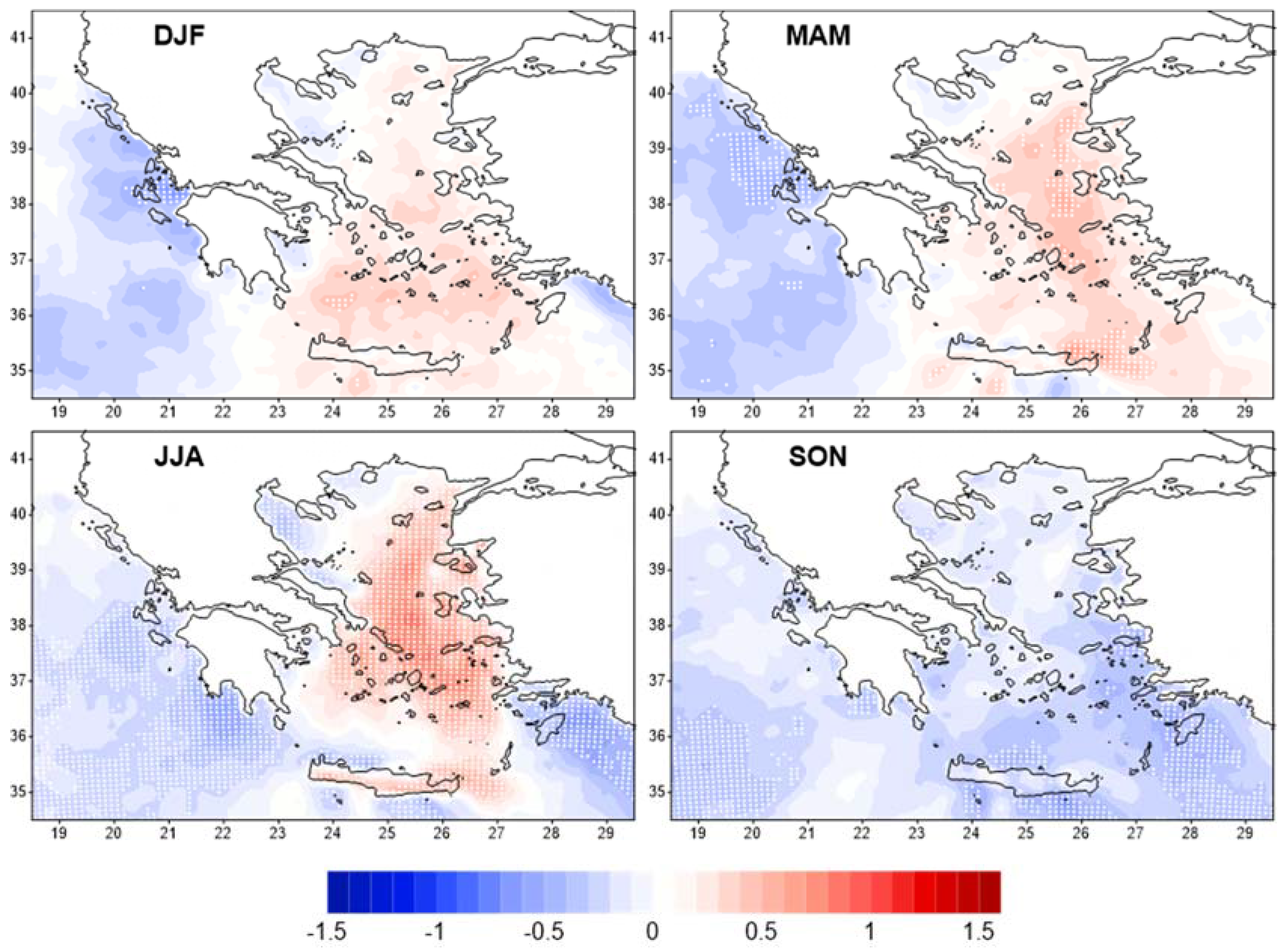
Figure 4 illustrates the biases between the mean wind speeds for the future period (2080–2100) and the control period (1980–2000). The future seasonal distribution of the prevailing wind directions is very similar to the control run distribution (not shown). On the other hand, statistically significant differences are detected in regards to the estimated future changes of the mean seasonal wind speeds. More specifically, future wind speeds perform in an opposite way between west (Aegean Sea) and east Greece.
In the western Aegean Sea, the mean seasonal wind speeds decrease during all seasons and statistical significant differences, up to −0.6 m/s, are observed during winter and spring, in the west coasts of the Greek mainland. During summer and autumn, a weaker decrease is observed, even though the areas characterized by statistically significant differences are more extended. Contrarily, wind speeds are expected to increase in the Aegean Sea from winter until summer. The only negative differences are observed during autumn. The highest increase is estimated to occur during summer in the central and northeast parts of the Aegean Sea (up to 0.8 m/s), while for winter, differences rarely exceed 0.4 m/s. During autumn, the observed decrease in wind speed exceeds −0.5 m/s in the south and the southeast Aegean Sea.
3.2.2. Extreme Wind Speed Thresholds
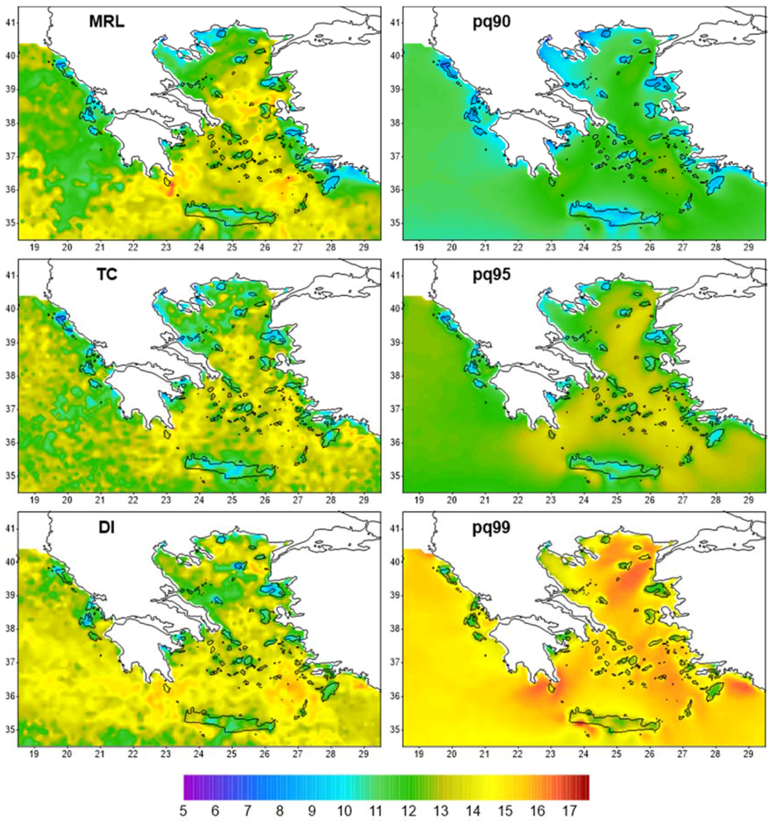
One of the main approaches in the extreme values theory is the Peak Over Threshold (POT) technique. Its advantages compared to the Block Maxima technique are the increased sample size and the decreased uncertainty of extreme values. An automated threshold selection approach was applied in this study in order to define extreme wind speed thresholds, based on three methods: the Mean Residual Life (MRL), the Threshold Choice (TC), and the Dispersion Index (DI). Additionally, extreme thresholds were defined using the statistical percentile procedure (90%, 95%, and 99%) with the aim of evaluating the results of the new procedure compared to those of a well-established procedure (Figure 5).
The application of the POT methods on RegCM3 data for the reference period gave thresholds comparable to those in the 95th percentile. Among the three POT methods, higher thresholds resulting from the DI method, however, do not have large differences from those of the other two methods. Higher threshold values are found in three regions of the Aegean Sea—the central Aegean Sea (above Cyclades), the sea between Peloponnese and Crete, and the sea between Cyclades and Dodecanese.
In order to minimize the uncertainties of each method, the mean threshold values of the three POT methods were estimated for each grid point in the study region (Figure 6). The southwest, as well as the southeast Aegean Sea, are the windiest regions over the Greek Seas, with threshold values up to 16 m/s. In the northeast Aegean Sea, threshold values are slightly lower (14 m/s–15 m/s). The lowest extreme thresholds occur in the northwest Aegean Sea, where they do not exceed 12.5 m/s.
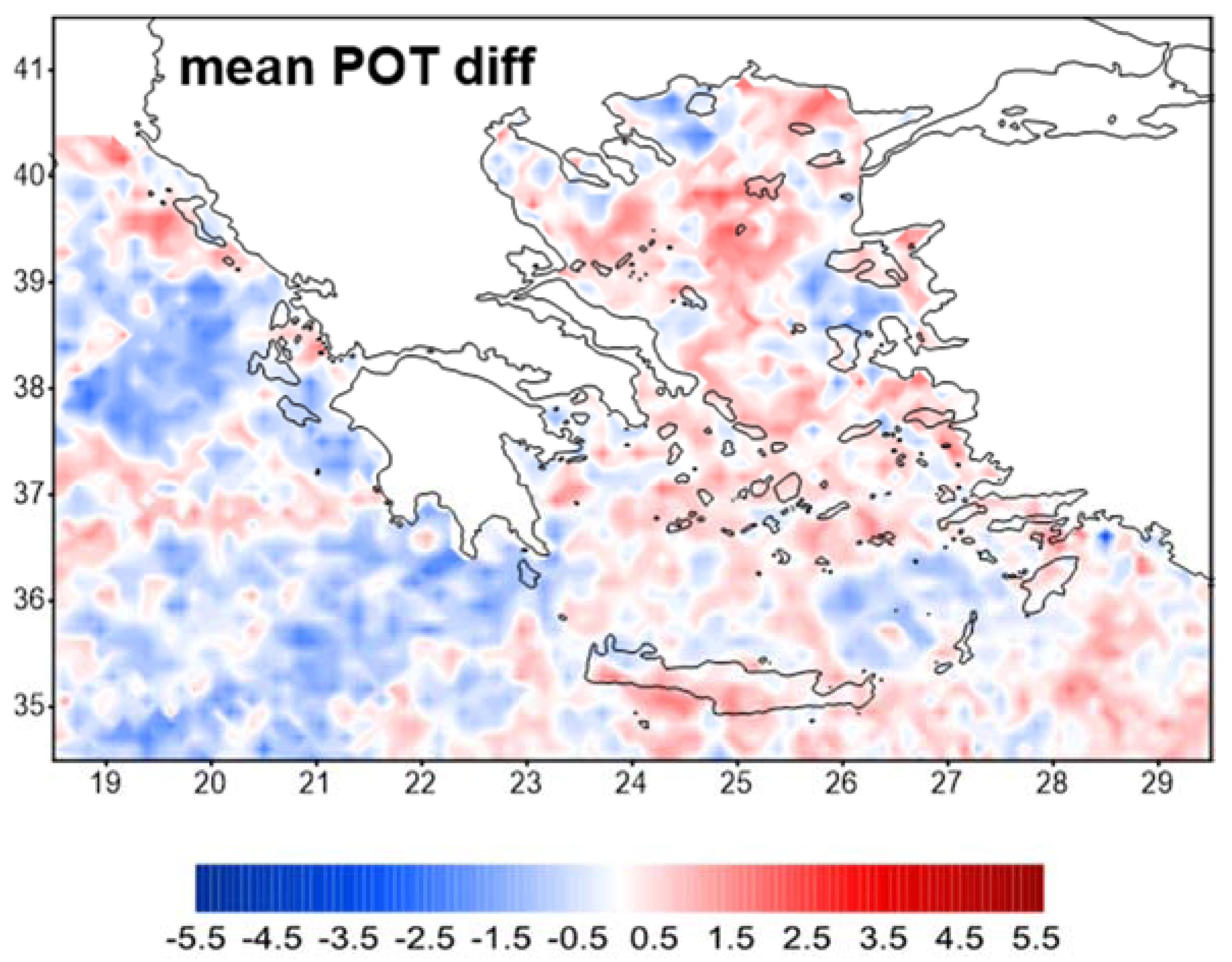
The geographical distribution of the mean POT threshold values bias between the control (1980–2000) and the future period (2080–2100) is illustrated in Figure 7. The average statistics of the RegCM3 10 km simulation show significant differences, both negative and positive, depending on the region. According to Figure 7, there is a “meridional” distribution of the biases. The longitude of 23° E can be considered as a boarder since regions west of it show a decrease of the extreme wind threshold for the future period, while regions to the east of this boarder present an increase. It should also be mentioned that future threshold values are expected to increase by 2 m/s and 1.5 m/s in the north and south Aegean Sea, respectively.
3.2.3. Seasonal Distribution of Extreme Winds
Based on the mean threshold values of the three POT methods, the seasonal frequencies of the excesses are estimated for each grid point (Figure 8). It is apparent that the highest frequencies are observed during winter. It is found that over half of the total excesses observed west of 22° E occur in winter. The rest of the cases are found mainly during autumn and spring. The temporal distribution of the frequencies of seasonal excesses for the Aegean Sea presents similarities to that of the Ionian Sea, meaning that a winter maximum and a summer minimum are observed even with some discrepancies in their spatial distribution.
More specifically, the lowest winter frequencies (30%–40%) of the excesses are observed in the central Aegean Sea surrounded by higher frequencies (more than 50%) especially in coastal areas and in the Ionian Sea. During spring, extreme wind frequencies are less than 30% in the largest part of the Aegean and north Ionian Seas, while frequencies higher than 20% are observed in the southern Ionian. Generally, for the majority of the regions of the Aegean Sea, the minimum frequencies are observed during summer, apart from the central and southern areas. In these regions, extreme wind cases occur more often in summer (Etesian winds) than in spring, with frequencies ranging from 20% to 40%. Percentages up to 40% are observed in most of the Aegean Sea during autumn, almost double compared to the frequencies observed in the Ionian Sea.
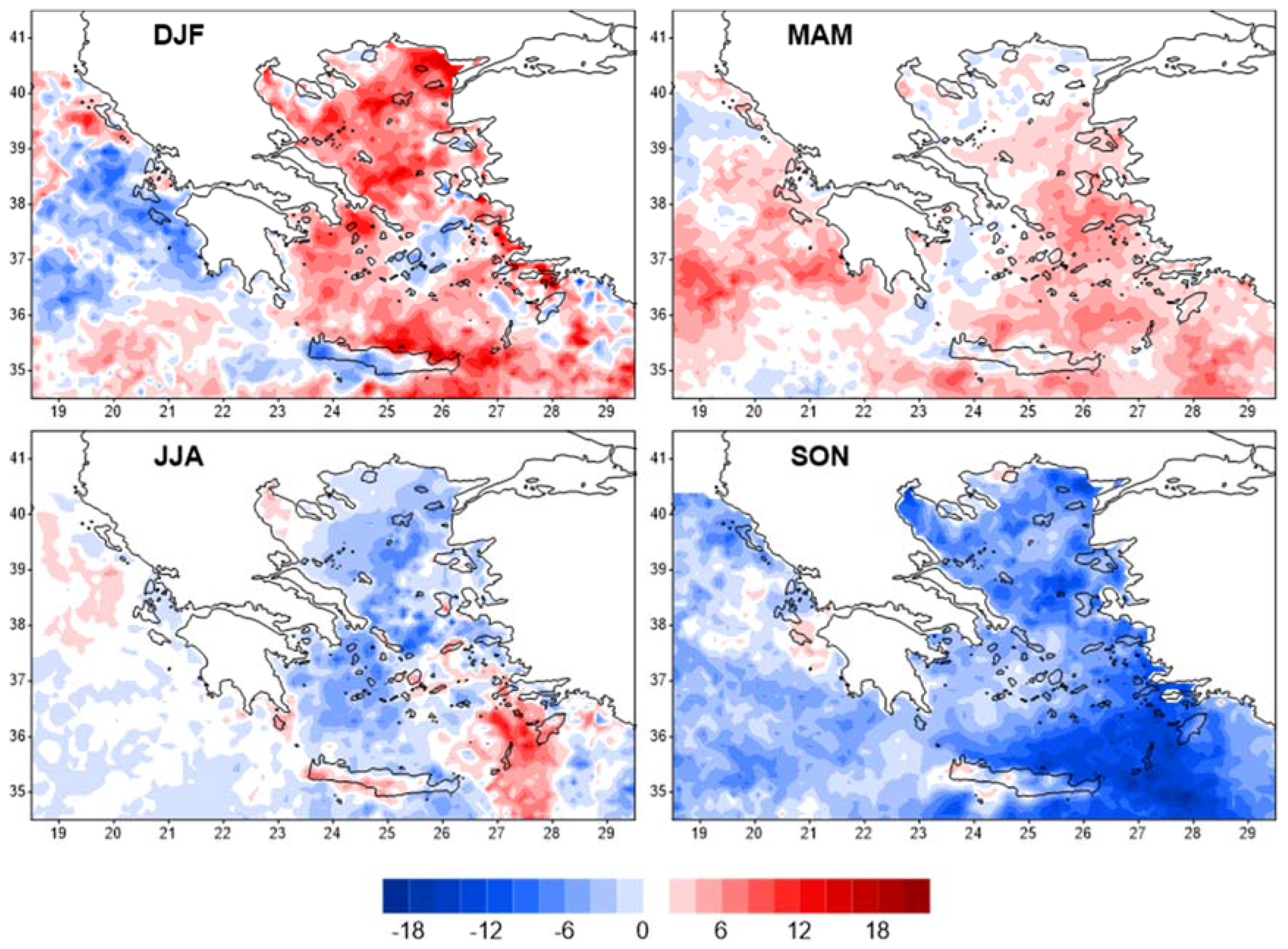
Figure 9 shows the magnitude of the frequency changes between the control and the future period. In the Aegean Sea, extreme winds will be more frequent during winter and spring. In detail, the winter change reaches 15% in the north and 10% in the south Aegean. During spring, the increase is lower, with the highest increase occurring in the central and southeast Aegean areas. In contrast, frequencies of extreme winds are expected to decrease in the Aegean Sea during summer and autumn. The negative differences do not exceed 10%, while a higher decrease (16%) is observed in the southeast Aegean in summer. This decrease of summer extreme wind frequencies in the southeast Aegean Sea is worth noticing, since it is observed in the region of the highest summer mean wind speeds. Furthermore, Figure 9 underlines the discrepancies between the eastern and western parts of Greece. In western Greece (Ionian Sea), negative differences prevail during autumn and winter, up to 10% and 15%, respectively. In spring, as in eastern Greece, there is an increase in extreme wind cases that reaches 12%, while frequencies similar to those of the control period are observed during summer.
3.2.4. Return Levels
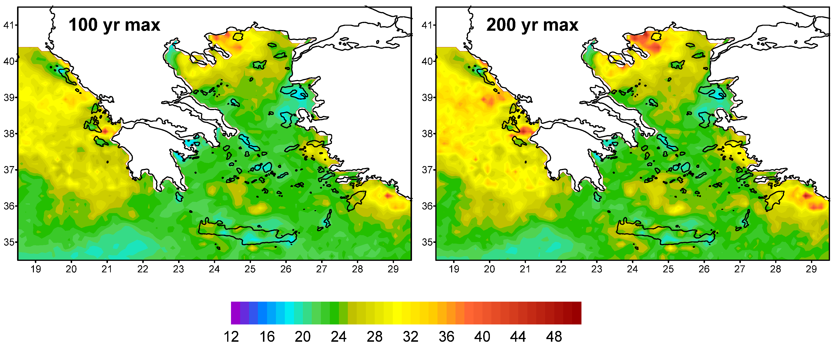
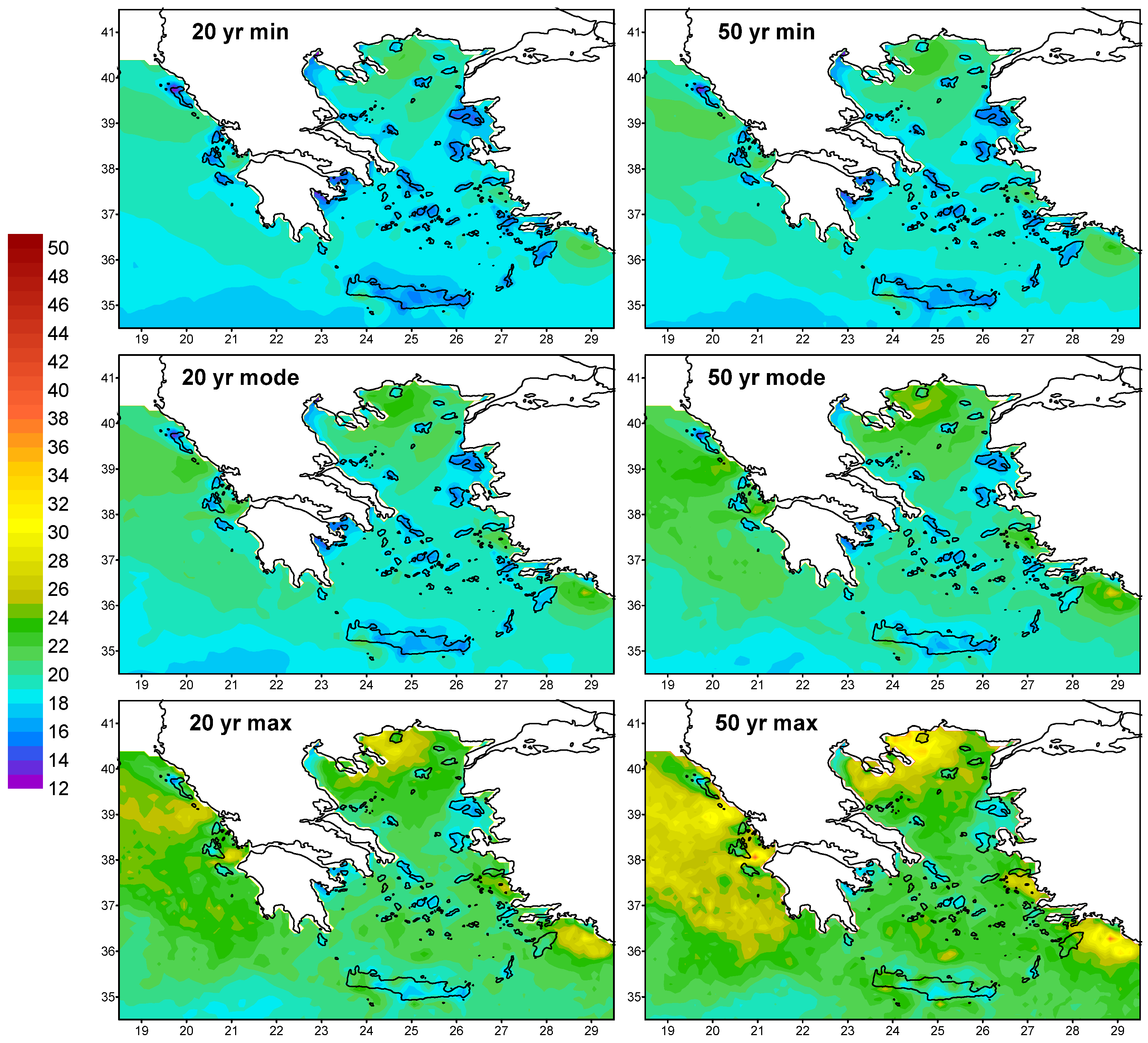
Return levels for 20, 50 100, and 200 year periods are estimated for the control period data, using the profile likelihood for the extreme excesses, as defined by the aforementioned POT approach. The 95% lower and upper confidence limits are also estimated. Figure 10 and Figure 11 summarize the different return level estimates (mode) and the 95% confidence intervals (min and max). It can be seen that the maxima of extreme winds are combined in three distinct regions, two of them located in the Aegean Sea (northern and southeastern parts) and the third one in the Ionian Sea (western coasts of Greece). On the contrary, the minima of the extreme winds are observed in the southwestern Greek region, between Peloponnese (southern Greek mainland) and the north coasts of Crete.
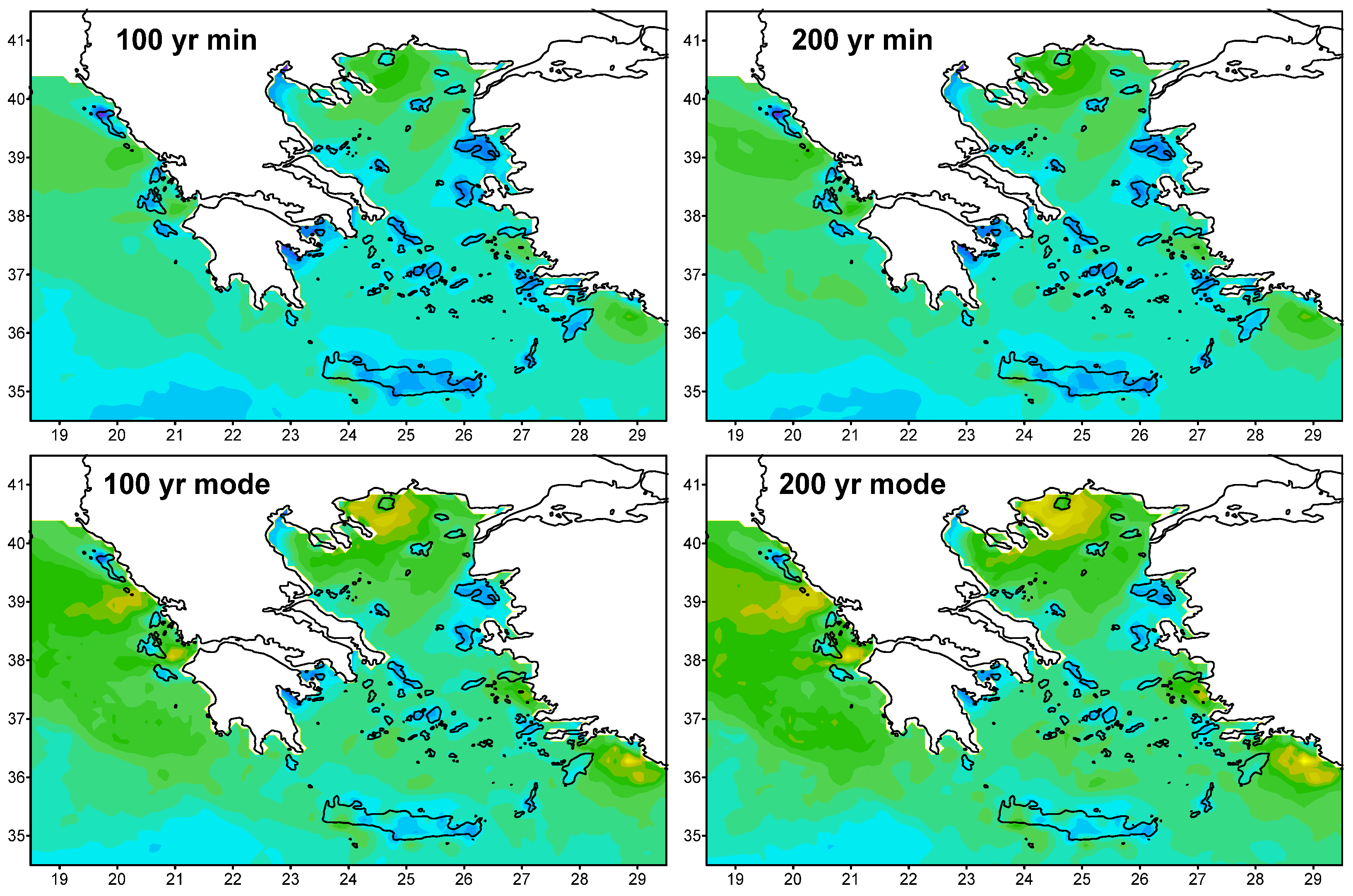
For the 20 year period (Figure 10), the return wind speed levels in the two Aegean regions are about 25 m/s. Winds speeds for the 50, 100, and 200 year periods (Figure 10 and Figure 11) seem to be approximately 2 m/s per period higher than those from the 20 year period. In the Ionian Sea, the maximum wind speed for the 20 year return period is 23 m/s, while for the 50, 100, and 200 year periods the increase of maximum wind speeds is about 3 m/s (50 year), 4 m/s (100 year), and 6 m/s (200 year).
4. Discussion
In this study, results from the high resolution (10 km) regional climate model (RegCM3) are used in order to study the marine surface wind (10 m) over the seas surrounding Greece. Such a high resolution is more suitable and should be preferred in order to “capture” and simulate the effects imposed by the complex coastlines and the numerous islands in the study region. The benefits of the 10 km spatial resolution have been highlighted in the study by [22], where results of the RegCM3’s 25 km and 10 km versions are compared. The 10 km version simulates wind speed better near sea-land alterations and during both winter and the summer Etesian period.
Comparisons with observation data from 15 meteorological stations, for the period 1980–2000, show good agreement with the model’s results. Prevailing wind directions rarely deviate from the observed ones throughout the year, since the wind direction is mainly a result of the general atmospheric circulation over the domain of study which in general is satisfactorily simulated by a regional climate model. On the other hand, the wind frequencies caused by stable atmospheric patterns are more efficiently reproduced by the model during the summer months while the west sector winds during winter and spring are rather overestimated. A possible explanation for this might be that the recurrent atmospheric circulation type over the study region every summer is attributed to the climatological stability of the persistent northerly winds.
The evaluation of the model’s skill in reproducing the median wind speeds is more complicated both in the case of the prevailing wind direction as well as for each direction separately. It seems that in some locations, especially in the Ionian Sea, the model systematically overestimates wind speed. Taking into account the excellent agreement of the 95th percentile wind speed between the RegCM3 and the observations, the differences in the median speeds need to be further investigated. A possible reason is the large number of calm days (daily wind speed less than 0.5 m/s) which are observed in the real data, in contrast with the model’s results where there are hardly any such values. In Alexandroupoli, Souda, Andravida, and Kerkyra, there are biases between observed and model data which could be attributed to the topographical surroundings and the “connection” of the station location (probably rough and elevated land) and the direction that most winds blow from. As mentioned by Pirazzoli and Tomasin [6], a differentiation in the behavior and time evolution (increasing or decreasing trend) in certain wind directions in a meteorological station could be attributed (apart from change in general circulation) also to local factors such as the building and vegetation changes and growth in the surrounding areas of the meteorological station. However, it should be noted that when Principal Component Analysis was employed, the simulated (model’s) and the observational results showed a very high level of agreement.
Regarding the simulated seasonal wind speeds, it was found that the highest values occur during winter in the largest part of the study region, with mean speeds higher than 8 m/s both in the Aegean and the Ionian Seas. Lower wind speeds are generally observed during summer in the Ionian and the north Aegean Sea, where the mean summer wind speed does not exceed 6.5 m/s. A notable exception is the southeast Aegean region, where the highest seasonal wind speeds reach 9.5 m/s (Etesian wind pattern). Similar wind speed magnitudes, for winter and summer of the 1961–2000 period, were estimated by [30] and the ensemble of the CLIM-RUN project [16]. However, the ensemble, which consists of RCM’s of 25 km spatial resolution, produced higher wind speed spread in the coasts (Greece, Turkey) and central Aegean in winter and central Aegean and north Crete coasts in summer, revealing the need for finer resolution models. In general, it should be mentioned that the RegCM3 model shows a higher simulating skill (in comparison to the observational data) during the warm period of the year and lowest simulating skill in winter. This could be attributed to the lower wind variability in summer due to a more “stable” atmospheric circulation over Greece and the existence of the Etesian Winds. Contrarily, during winter, the atmospheric circulation presents a higher variability due to the frequent alternations of the barometric systems that influence and change the flow of the surface winds.
Future wind speed differences ((2080–2100)–(1980–2000)) are expected to show a decrease in the Ionian Sea during all seasons. Conversely, in the largest part of the Aegean Sea the seasonal wind speeds are projected to increase from winter until summer, while the future autumn wind speeds will be weaker. The strengthening of the Etesians should be highlighted, with statistically significant increases in wind speed observed in all of the east Aegean regions during summer [29,30], which is associated with the reinforcement of the high pressure system over the Balkan Peninsula and the deepening of the Asiatic thermal low over the eastern Mediterranean. Moreover, Mclnnes et al. [32] showed in their study that more than 2/3 out of the 19 GCMs that they incorporated agree on a future increase of the Etesian winds all over the Aegean region too, while on the other hand they concluded that there would be a decrease in the mean wind speeds over the central Ionian Sea.
Finally, in the case of the extreme winds analysis, the extreme wind speed thresholds were estimated using three Peaks Over Threshold methods. Van de Vyver and Delcloo [33] highlighted the advantage of the POT method over the Block maxima for extreme wind gusts in Belgium. On the other hand, Caires [34] writes that generally POT estimates are more accurate than the corresponding Block maxima, but that when the time period is longer than 200 years the accuracies of the two approaches are similar, It was found that the mean threshold values are slightly higher than the 95th percentile wind speed values. The highest thresholds were observed in the southeast and the southwest Aegean Sea, while another center of high threshold values covers the northeast Aegean. Future changes in extreme speeds show a general decrease in the Ionian Sea, while higher thresholds are expected in the Aegean Sea. These results are in agreement with the changes in projected mean wind speeds, further validating the suitability of the POT methods in estimating extreme wind speed thresholds. Analogous results were found in the Rockel and Worth [12] study which considered two RCMs that include a diagnostic gust parameterization; their showed that in the future period (2071–2100) the frequency of occurrence of winds higher than 8 Bft will decrease in the Ionian and the northwestern Aegean Sea, while a future increase is estimated in the rest of the Aegean Sea. A decrease of the 98th percentile of the wind speeds over the southern Ionian Sea was also detected in the Pinto et al. [35] study, which used a CHAM5.MPI-OM1 GCM. Mclnnes et al. [32] also indicated that even the 99th percentile of mean wind speed is also expected to decrease in the Ionian Sea during the last 20 years of the 21st century.
The seasonal excesses over the estimated mean POT thresholds constitute the extreme winds produced by the RegCM3. Their intra-annual distribution shows that the highest extreme wind frequencies occur during winter, at the coastal regions of Greece and Turkey. Off shore regions of the Ionian Sea also are subjected to frequent extreme winds during the same period of the year. In the rest of the Aegean Sea, the majority of extreme wind cases are expected both in autumn and winter. The effect of the Etesian pattern is once again distinguished during summer in the central and southeastern Aegean Sea, where the only notable extreme wind frequencies are observed during this season. In the future, extreme winds are expected more often during winter and spring in the Aegean Sea and during spring in the Ionian. In contrast, less extreme winds are expected during summer to autumn and during winter, for the Aegean Sea and the Ionian Sea, respectively. However, despite the decline of extreme cases in most of the Aegean Sea during summer, an increase is expected in its southeastern part.
The largest changes in the return levels occur in the northern and southeastern Aegean Sea and Ionian Sea regions. In these regions, the 100-year return level ((200-)f extreme wind maxima increase by more than 6 m/s (10 m/s), an increase that could have severe impacts along the coastal regions. Over the Ionian Sea and northern Aegean Sea, this increase is more than 100% compared to the present-day climate. According to Makris et al. [36], in these two regions, the Storm Surge Index (SSI) presents the highest values underling the vulnerability of these coastal areas. Moreover, Krestenitis et al. [37] showed that the southeastern Aegean Sea presents an increase of the frequency of Sea Level High (SLH) during the recent years.
5. Conclusions
This study set out to evaluate the ability of the high resolution (10 km) regional climate model (RegCM3) in capturing the main characteristics of the marine surface wind over the Greek Seas. Moreover, an attempt was made to define extreme wind speed thresholds for the Aegean and Ionian Seas. The main conclusions drawn from the present study are:
- The high resolution (10 km) regional climate model (RegCM3) successfully captures the characteristic of the marine surface wind over the Greeks Seas.
- The model considered in this paper can successfully simulate the prevailing wind directions during the time periods when stability of the atmospheric circulation is observed (mainly during the summer months).
- Topography and local factors (buildings and vegetation) in the surrounding areas of the meteorological station can restrain the ability of the model to project the wind direction.
- The highest seasonal wind speeds occur during winter and are higher than 8 m/s over the Greek Seas.
- Wind speed is expected to decrease in the Ionian Sea at the end of the 21st century, while seasonal wind speeds will increase in the Aegean Sea during all seasons except autumn.
- The windiest regions over the Greek Seas are the southwest and the southeast Aegean Sea, with extreme threshold value up to 16 m/s. For the future, extreme wind speeds are expected to increase by 2 m/s in the north and 1.5 m/s in the south Aegean Sea, , and decrease in Ionian Sea.
- The highest seasonal excesses over the extreme wind thresholds are observed at the coastal regions of Greece and Turkey during winter, while the excesses move to the central and southeastern Aegean Sea during summer.
- The extreme wind values for 20, 50, 100, and 200-return periods were estimated. The largest changes in the return levels will occur in Northern Aegean Sea and Ionian Sea.
Further studies, which take these variables into account, will need to be undertaken, using the new Representative Concentration Pathways RCPs scenarios.
Acknowledgments
This research has been co-financed by the European Union (European Social Fund (ESF)) and Greek national funds through the Operational Program BEducation and Lifelong Learning of the National Strategic Reference Framework (NSRF)—Research Funding Program: Thales. Investing in knowledge society through the European Social Fund (Project CCSEAWAVS: Estimating the effects of Climate Change on SEA level and WAve climate of the Greek seas, coastal Vulnerability and Safety of coastal and marine structures). Results presented in this work have been produced using the AUTH Compute Infrastructure and Resources.
Author Contributions
All authors conceived and initiated the study. Christina Anagnostopoulou and Konstantia Tolika downscaled the RegCM data to 10 km×10 km resolution. Christos Vagenas analyzed the data. All authors contributed to the discussion and interpretation of the results and the writing of the manuscript.
Conflicts of Interest
The authors declare no conflict of interest.
References
- Kubota, M.; Yokota, H.J. Oceanogr Construction of surface wind stress fields with high temporal resolution using ERS-1. Scatt. Data 1998, 54, 247. [Google Scholar]
- Zecchetto, S.; Cappa, C. The spatial structure of the Mediterranean Sea winds revealed by ERS-1 scatterometer. Int. J. Remote Sens. 2001, 22, 45–70. [Google Scholar] [CrossRef]
- Seneviratne, S.I.; Nicholls, N.; Easterling, D.; Goodess, C.M.; Kanae, S.; Kossin, J.; Luo, Y.; Marengo, J.; McInnes, K.; Rahimi, M.; et al. Changes in climate extremes and their impacts on the naturalphysical environment. In Managing the Risks of Extreme Events and Disasters to Advance Climate Change Adaptation: A Special Report of Working Groups I and II of the Intergovernmental Panel on Climate Change (IPCC); Field, C.B., Barros, V., Stocker, T.F., Qin, D., Dokken, D.J., Ebi, K.L., Mastrandrea, M.D., Mach, K.J., Plattner, G.-K., Allen, S.K., et al., Eds.; Cambridge University Press: Cambridge, UK; New York, NY, USA, 2012; pp. 109–230. [Google Scholar]
- Mcvicar, T.R.; Van Niel, T.G.; Li, L.T.; Roderick, M.L.; Rayner, D.P.; Ricciardulli, L.; Donohue, R.J. Wind speed climatology and trends for Australia, 1975–2006: Capturing the stilling phenomenon and comparison with near surface reanalysis output. Geophys. Res. Lett. 2008, 35, 288–299. [Google Scholar] [CrossRef]
- McLnnes, K.L.; Macadam, I.; Hubbert, G.D.; O’Grady, J.G. A modeling approach for estimating the frequency of sea level extrems and the impact of climate change in southeast Australia. Nat. Hazards 2009, 51, 115–137. [Google Scholar] [CrossRef]
- Pirazzoli, P.A.; Tomasin, A. Recent near-surface wind changes in the central Mediterranean and Adriatic areas. Int. J. Climatol. 2003, 23, 963–973. [Google Scholar] [CrossRef]
- Sotillo, M.G.; Ratsimandresy, A.W.; Carretero, J.C.; Bentamy, A.; Valero, F.; González-Rouco, F. A high-resolution 44-year atmospheric hindcast for the Mediterranean Basin: contribution to the regional improvement of global reanalysis. Clim. Dyn. 2005, 25, 219–236. [Google Scholar] [CrossRef]
- Winterfeldt, J.; Andersson, A.; Klepp, C.; Bakan, S.; Weisse, R. Comparison of HOAPS, QuikSCAT and buoy wind speed in the eastern North Atlantic and the North Sea. IEEE Trans. Geosci. Remote Sens. 2010, 48, 338–348. [Google Scholar] [CrossRef]
- Zecchetto, S.; de Biasio, F. Sea surface winds over the Mediterranean basin from satellite data (2000–2004): Meso- and local-scale features on annual and seasonal time scales. J. Appl. Meteorol. Climatol. 2007, 46, 814–827. [Google Scholar] [CrossRef]
- IPCC: Managing the Risks of Extreme Events and Disasters to Advance Climate Change Adaptation. A Special Report of Working Groups I and II of the Intergovernmental Panel on Climate Change; Field, C.B.; Barros, V.; Stocker, T.F.; Qin, D.; Dokken, D.J.; Ebi, K.L.; Mastrandrea, M.D.; Mach, K.J.; Plattner, G.-K.; Allen, S.K.; et al. (Eds.) Cambridge University Press: Cambridge, UK; New York, NY, USA, 2012; p. 582. [Google Scholar]
- Weisse, R.; von Storch, H.; Feser, F. Northeast Atlantic and North Sea storminess as simulated by a regional climate model 1958–2001 and comparison with observations. J. Clim. 2005, 18, 465–479. [Google Scholar] [CrossRef]
- Rockel, B.; Woth, K. Extrems of near surface wind speeds over Europe and their future changes as estimated from an ensemble of RCM simulations. Clim. Chang. 2007, 81, 267–280. [Google Scholar] [CrossRef]
- Beniston, M.; Stephenson, D.B.; Christensen, O.B.; Ferro, C.A.T.; Frei, C.; Goyette, S.; Halsnaes, K.; Holt, T.; Jylhä, K.; Koffi, B.; et al. Future extreme events in European climate: an exploration of regional climate model projections. Clim. Chang. 2007, 81 (Suppl. 1), 71–95. [Google Scholar] [CrossRef]
- Haugen, J.E.; Iversen, T. Response in extremes of daily precipitation and wind from a downscaled multimodel ensemble of anthropogenic global climate change scenarios. Tellus 2008, 60, 411–426. [Google Scholar] [CrossRef]
- Rauthe, M.; Kunz, M.; Kottmeier, C. Changes in wind gust extremes over Central Europe derived from a small ensemble of high resolution regional climate models. Meteorol. Z. 2010, 19, 299–312. [Google Scholar]
- Bellucci, A.; Gualdi, S.; Masina, S.; Storto, A.; Scoccimarro, E.; Cagnazzo, C.; Fogli, P.; Manzini, E.A.; Navarra, A. Decadal climate predictions with a coupled OAGCM initialized with oceanic reanalyses. Clim. Dyn. 2013, 40, 1483–1497. [Google Scholar] [CrossRef]
- Walshaw, D. Modelling extreme wind speeds in regions prone to hurricanes. Appl. Stat. 2000, 49, 51–62. [Google Scholar] [CrossRef]
- Sheskin, D.J. Handbook of Parametric and Nonparametric Statistical Procedures; CRC Press: Boca Raton, FL, USA, 2003; p. 1192. [Google Scholar]
- Anagnostopoulou, C.; Tolika, K. Extreme precipitation in Europe: Statistical threshold selection based on climatological criteria. Theor. Appl. Climatol. 2011, 107, 479–489. [Google Scholar] [CrossRef]
- Emanuel, K.A. A scheme for representing cumulus convection in large-scale models. J. Atmos. Sci. 1991, 48, 2313–2329. [Google Scholar] [CrossRef]
- Emanuel, K.A.; Lvkovic-Rothman, M. Development and evaluation of a convective scheme for use in climate models. J. Atmos. Sci. 1999, 48, 1766–1782. [Google Scholar] [CrossRef]
- Tolika, K.; Anagnostopoulou, C.; Velikou, K.; Vagenas, C. A comparison of the updated very high resolution model RegCM3_10 km with the previous version RegCM3_25 km over the complex terrain of Greece: Present and future projections. Theor. Appl. Climatol. 2016, 126, 715–726. [Google Scholar] [CrossRef]
- Thomas, B.; Kent, E.; Swail, V.; Berry, D. Trends in ship wind speeds adjusted for observation method and height. Int. J. Climatol. 2008, 28, 747–763. [Google Scholar] [CrossRef]
- Coles, S. An Introduction to Statistical Modeling of Extreme Values; Springer: Berlin/Heidelberg, Germany, 2001. [Google Scholar]
- Davison, A.C.; Smith, R.L. Models for exceedances over high thresholds. J. R. Stat. Soc. Ser. B 1990, 52, 393–442. [Google Scholar]
- Scarrott, C.; Macdonald, A. A review of extreme value threshold es-timation and uncertainty quantification. REVSTAT–Stat. J. 2012, 10, 33–60. [Google Scholar]
- Ribatet, M. POT: Modelling peaks over a threshold. Threshold 2007, 5, 15–30. [Google Scholar]
- Begueria, S. Uncertainties in partial duration series modelling of extrems related to the choice of the threshold value. J. Hydrol. 2005, 303, 215–230. [Google Scholar] [CrossRef]
- Anagnostopoulou, C.; Zanis, P.; Katragkou, E.; Tegoulias, I.; Tolika, K. Resent past and future patterns of the Etesian winds based on regional scale climate model simulations. Clim. Dyn. 2014, 42, 1819–1836. [Google Scholar] [CrossRef]
- Tyrlis, E.; Lelieveld, J. Climatology and dynamics of the summer Etesian Winds over the Eastern Mediterranean. J. Atmos. Sci. 2013, 70, 3374–3396. [Google Scholar] [CrossRef]
- Bloom, A.; Kotroni, V.; Lagouvardos, K. Climate change impact of wind energy availability in the Eastern Mediterranean using the regional climate model PRECIS. Nat. Hazards Earth Syst. Sci. 2008, 8, 1249–1257. [Google Scholar] [CrossRef]
- Mclnnes, K.l.; Erwin, T.A.; Bathols, J.M. Global Climate Model projected changes in 10m wind speed and diraction due to anthropogenic climate change. Atmos. Sci. Lett. 2011, 12, 325–333. [Google Scholar] [CrossRef]
- Van De Vyver, H.; Delcloo, A.W. Stable estimations for extreme wind speeds. An application to Belgium. Theor. Appl. Climatol. 2011, 105, 417–429. [Google Scholar] [CrossRef]
- Caires, S. A Comparative Simulation Study of the Annual Maxima and the Peaks over-Threshold Methods. J. Offshore Mech. Arct. Eng. 2016, 138, 051601. [Google Scholar] [CrossRef]
- Pinto, J.G.; Ulbrich, U.; Leckebusch, G.C.; Spangehl, T.; Reyers, M.; Zacharias, S. Changes in storm track and cyclone activity in three SRES ensemble experiments with the ECHAM5/MPI-OM1 GCM. Clim. Dyn. 2009, 29, 195–210. [Google Scholar] [CrossRef]
- Makris, C.; Galiatsatou, P.; Tolika, K.; Anagnostopoulou, C.; Kombiadou, K.; Prinos, P.; Velikou, K.; Kapelonis, Z.; Tragou, E.; Androulidakis, Y.; et al. Climate change effects on the marine characteristics of the Aegean and Ionian Seas. Ocean Dyn. 2016, 66, 1603–1635. [Google Scholar] [CrossRef]
- Krestenitis, Y.N.; Androulidakis, Y.S.; Kontos, Y.N.; Georgakopoulos, G. Coastal inundation in the north-eastern Mediterranean coastal zone due to storm surge events. J. Coast. Conserv. 2011, 15, 353–368. [Google Scholar] [CrossRef]
Figure 1.
The 15 Greek meteorological stations in the Aegean Sea and the Ionian Sea.

Figure 2.
Principal component loadings of the first four PCs of the winter Principal Component Analysis (PCA), for the model (left) and the stations’ (right) data.
Figure 2.
Principal component loadings of the first four PCs of the winter Principal Component Analysis (PCA), for the model (left) and the stations’ (right) data.
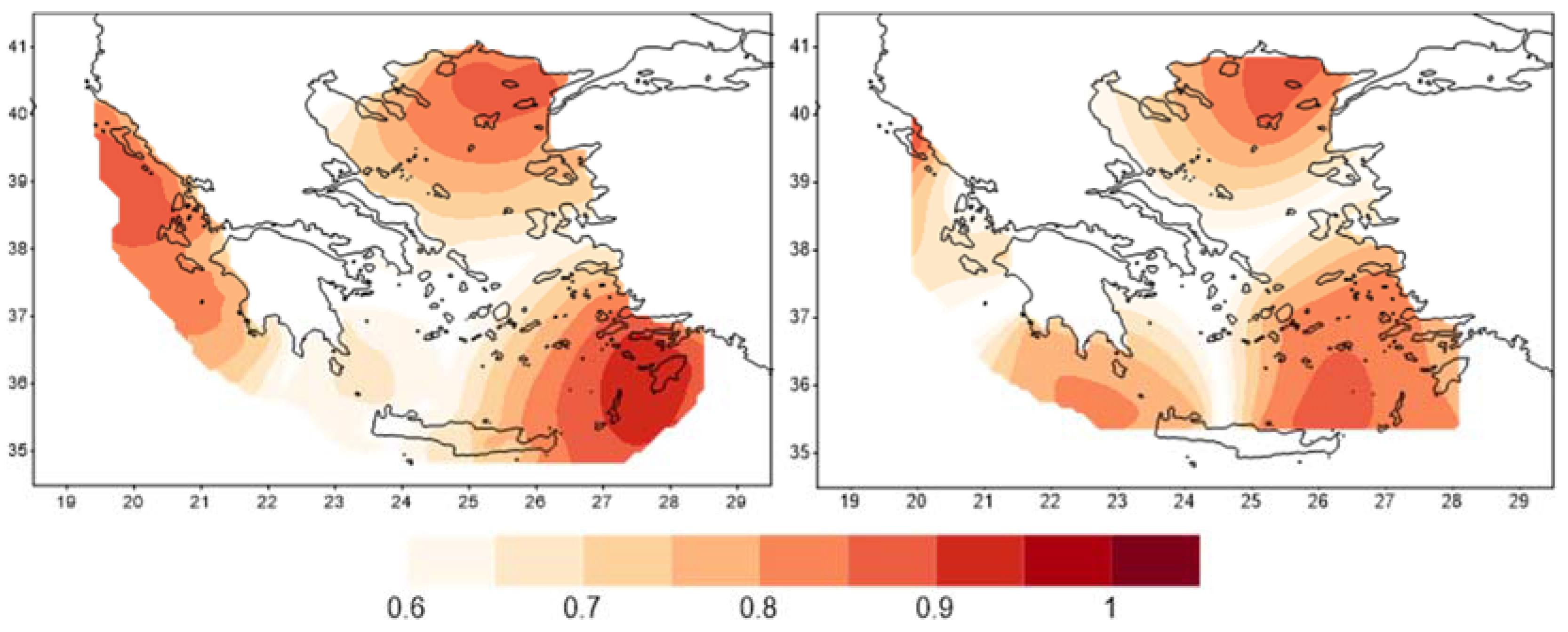
Figure 3.
Mean seasonal wind speed in m/s (colored scale) and prevailing seasonal wind direction (arrows) of the RegCM3 data for 1980–2000. DJF is for winter; MAM for spring; JJA for summer and SON for autumn.
Figure 3.
Mean seasonal wind speed in m/s (colored scale) and prevailing seasonal wind direction (arrows) of the RegCM3 data for 1980–2000. DJF is for winter; MAM for spring; JJA for summer and SON for autumn.
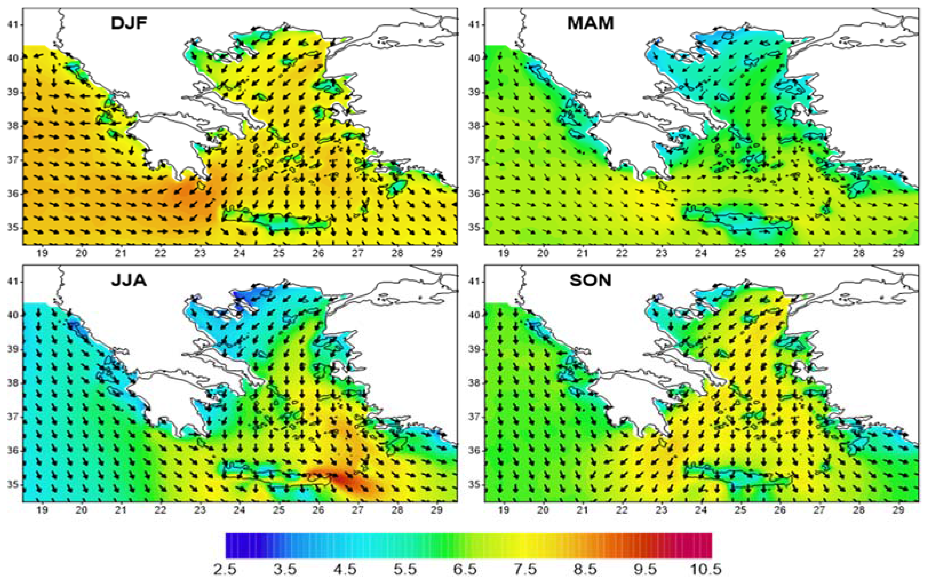
Figure 4.
Mean seasonal wind speed differences in m/s for the period 2080–2100 compared to the 1980–2000 period. Statistical significant differences are denoted with white dots. DJF is for winter; MAM for spring; JJA for summer and SON for autumn.
Figure 4.
Mean seasonal wind speed differences in m/s for the period 2080–2100 compared to the 1980–2000 period. Statistical significant differences are denoted with white dots. DJF is for winter; MAM for spring; JJA for summer and SON for autumn.

Figure 5.
Extreme wind speed thresholds in m/s (color scale) as estimated by the three Peak Over Threshold (POT) methods (left column) and the three percentile indices (right column) for the period 1980–2000.
Figure 5.
Extreme wind speed thresholds in m/s (color scale) as estimated by the three Peak Over Threshold (POT) methods (left column) and the three percentile indices (right column) for the period 1980–2000.

Figure 6.
Mean extreme wind speed thresholds in m/s of the three POT methods for the period 1980–2000.
Figure 6.
Mean extreme wind speed thresholds in m/s of the three POT methods for the period 1980–2000.
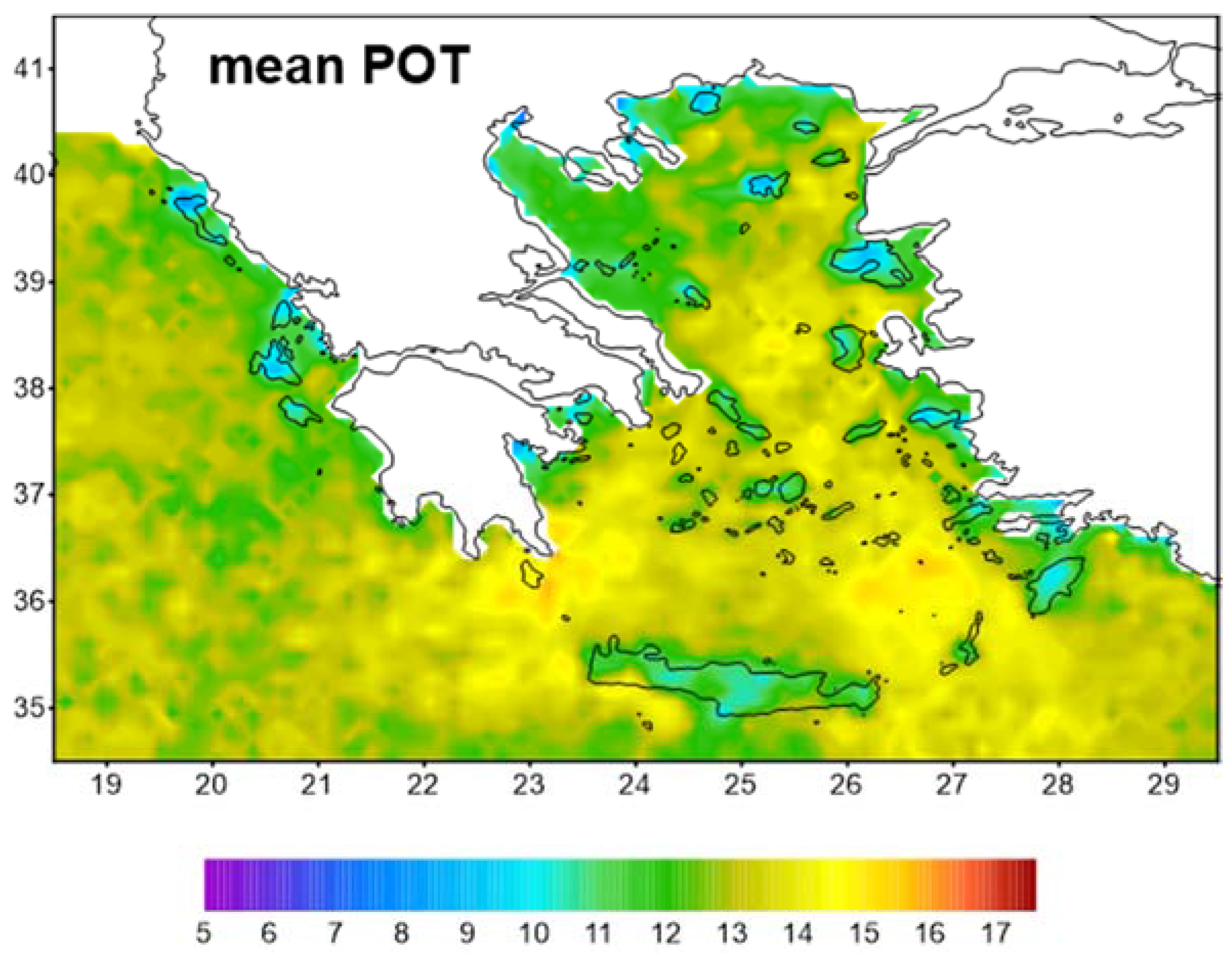
Figure 7.
Differences in mean extreme wind speed thresholds in m/s of the three POT methods for the period 2080–2100 compared to the 1980–2000 period.
Figure 7.
Differences in mean extreme wind speed thresholds in m/s of the three POT methods for the period 2080–2100 compared to the 1980–2000 period.

Figure 8.
Mean seasonal extreme wind speed frequencies (%) for the period 1980–2000. DJF is for winter; MAM for spring; JJA for summer and SON for autumn.
Figure 8.
Mean seasonal extreme wind speed frequencies (%) for the period 1980–2000. DJF is for winter; MAM for spring; JJA for summer and SON for autumn.

Figure 9.
Differences in mean seasonal extreme wind speed frequencies for the period 2080–2100 compared to the 1980–2000 period. DJF is for winter; MAM for spring; JJA for summer and SON for autumn.
Figure 9.
Differences in mean seasonal extreme wind speed frequencies for the period 2080–2100 compared to the 1980–2000 period. DJF is for winter; MAM for spring; JJA for summer and SON for autumn.

Figure 10.
Return wind speed levels in m/s for 20 (left column) and 50 (right column) year periods (mode) and 95% lower (min) and upper (max) confidence limits, as estimated by the profile likelihood, based on the RegCM3 data for the 1980–2000 period.
Figure 10.
Return wind speed levels in m/s for 20 (left column) and 50 (right column) year periods (mode) and 95% lower (min) and upper (max) confidence limits, as estimated by the profile likelihood, based on the RegCM3 data for the 1980–2000 period.

Figure 11.
As Figure 10, but for 100 (left column) and 200 (right column) year periods.
Figure 11.
As Figure 10, but for 100 (left column) and 200 (right column) year periods.


Table 1.
The explained variance of the first four Principal Components PCs for station and model data in seasonal base.
Table 1.
The explained variance of the first four Principal Components PCs for station and model data in seasonal base.
| Station | Model | |
|---|---|---|
| Winter | 78.5 | 92.0 |
| Spring | 74.4 | 90.1 |
| Summer | 77.7 | 89.6 |
| Autumn | 76.1 | 90.8 |
Table 2.
Biases between station and grid point data for prevailing wind direction (degrees), frequency of prevailing wind direction, median speed of prevailing direction (m/s), median wind speed (m/s), and 95th percentile of wind speed (m/s). The color scale is as follows: biases less than 2 m/s: blue; 1 m/s–2 m/s: light blue; −1 m/s to 1 m/s: yellow; 1 m/s–2 m/s: orange and greater than 2 m/s: brown. The color scale of the frequency of prevailing wind direction is similar but the thresholds are multiples of ten.
| NE Aegean | SE Aegean | SW Aegean | Ionian | |||||||||||||
|---|---|---|---|---|---|---|---|---|---|---|---|---|---|---|---|---|
| Alex/Poli | Lemnos | Skyros | Mytilene | Naxos | Samos | Rhodes | Heraklion | Milos | Souda | Kythira | Methoni | Andravida | Aktio | Kerkyra | ||
| Prevailing wind direction | DJF | 0 | 0 | 0 | 0 | 0 | 0 | 0 | 0 | 0 | 0 | 0 | 0 | 180 | 45 | 0 |
| MAM | 0 | 0 | 0 | 0 | 0 | 0 | 0 | 0 | 0 | −45 | −135 | 0 | −45 | −90 | 0 | |
| JJA | 0 | 0 | 0 | 0 | 0 | 0 | 45 | 0 | 0 | 0 | −90 | 0 | 0 | −45 | 0 | |
| SON | 0 | 0 | 45 | 45 | 0 | 0 | 45 | 0 | 0 | 0 | 0 | 0 | 45 | 180 | 0 | |
| Frequency of prevailing wind direction | DJF | |||||||||||||||
| MAM | ||||||||||||||||
| JJA | ||||||||||||||||
| SON | ||||||||||||||||
| Median speed of prevailing wind direction | DJF | |||||||||||||||
| MAM | ||||||||||||||||
| JJA | ||||||||||||||||
| SON | ||||||||||||||||
| Median wind speed | DJF | |||||||||||||||
| MAM | ||||||||||||||||
| JJA | ||||||||||||||||
| SON | ||||||||||||||||
| 95th percentile of wind speed | DJF | |||||||||||||||
| MAM | ||||||||||||||||
| JJA | ||||||||||||||||
| SON | ||||||||||||||||
© 2017 by the authors. Licensee MDPI, Basel, Switzerland. This article is an open access article distributed under the terms and conditions of the Creative Commons Attribution (CC BY) license (http://creativecommons.org/licenses/by/4.0/).
Share and Cite
MDPI and ACS Style
Vagenas, C.; Anagnostopoulou, C.; Tolika, K. Climatic Study of the Marine Surface Wind Field over the Greek Seas with the Use of a High Resolution RCM Focusing on Extreme Winds. Climate 2017, 5, 29. https://doi.org/10.3390/cli5020029
AMA Style
Vagenas C, Anagnostopoulou C, Tolika K. Climatic Study of the Marine Surface Wind Field over the Greek Seas with the Use of a High Resolution RCM Focusing on Extreme Winds. Climate. 2017; 5(2):29. https://doi.org/10.3390/cli5020029
Chicago/Turabian StyleVagenas, Christos, Christina Anagnostopoulou, and Konstantia Tolika. 2017. "Climatic Study of the Marine Surface Wind Field over the Greek Seas with the Use of a High Resolution RCM Focusing on Extreme Winds" Climate 5, no. 2: 29. https://doi.org/10.3390/cli5020029
Note that from the first issue of 2016, this journal uses article numbers instead of page numbers. See further details here.