
Application of Satellite-Based Precipitation Estimates to Rainfall-Runoff Modelling in a Data-Scarce Semi-Arid Catchment


1
Department of Geography, Centre for Landscape and Climate Research, University of Leicester, Leicester LE1 7RH, UK
2
Department of Soil and Water Science, Faculty of Agricultural Sciences, University of Sulaimani, Iraq-Kurdistan Region-Sulaimani-Bekrajo 46011, Iraq
3
National Centre for Earth Observation, University of Leicester, Leicester LE1 7RH, UK
*
Author to whom correspondence should be addressed.
Climate 2017, 5(2), 32; https://doi.org/10.3390/cli5020032
Submission received: 7 March 2017
/
Revised: 29 March 2017
/
Accepted: 30 March 2017
/
Published: 11 April 2017
(This article belongs to the Special Issue Using Tropical Rainfall Measuring Mission (TRMM) Data in Research and Applications)
Abstract
:Rainfall-runoff modelling is a useful tool for water resources management. This study presents a simple daily rainfall-runoff model, based on the water balance equation, which we apply to the 11,630 km2 Lesser Zab catchment in northeast Iraq. The model was forced by either observed daily rain gauge data from four stations in the catchment or satellite-derived rainfall estimates from two TRMM Multi-satellite Precipitation Analysis (TMPA) data products (TMPA-3B42 and 3B42RT) based on the Tropical Rainfall Measuring Mission (TRMM) from 2003 to 2014. As well as using raw TMPA data, we used a bias-correction method to adjust TMPA values based on rain gauge data. The uncorrected TMPA data products underestimated observed mean catchment rainfall by −10.1% and −10.7%. Corrected data also slightly underestimated gauged rainfall by −0.7% and −1.6%, respectively. Nash-Sutcliffe Efficiency (NSE) and Pearson’s Correlation Coefficient (r) for the model fit with the observed hydrograph were 0.75 and 0.87, respectively, for a calibration period (2010–2011) using gauged rainfall data. Model validation performance (2012–2014) was best (highest NSE and r; lowest RMSE and bias) using the corrected 3B42 data product and poorest when driven by uncorrected 3B42RT data. Uncertainty and equifinality were also explored. Our results suggest that TRMM data can be used to drive rainfall-runoff modelling in semi-arid catchments, particularly when corrected using rain gauge data.
1. Introduction
Understanding and modelling hydrological processes is important for the management of water resources and for the analysis of extreme hydrological events, such as droughts or floods. However, a significant issue with many semi-arid zones outside of Europe and North America is that meteorological and hydrological data availability is often scarce. Some of the problems associated with obtaining reliable long-term hydrological data in semi-arid regions include limited economic resources for monitoring, sparse population and harsh climates [1,2]. This is compounded by the fact that spatial and temporal variability in hydrological activity can be much higher than in humid temperate areas, requiring (in principle) denser monitoring networks (e.g., rain gauges and streamflow gauging stations) to capture the nature of system behaviour [3,4,5]. This issue is even more acute in mountainous areas where spatial and temporal variability in precipitation tends to be higher than in lowland areas. Unfortunately, the establishment and maintenance of such networks is often not a priority for many developing countries or is quite simply unaffordable. Even when monitoring data exist, they may be of variable quality, contain significant gaps or be unavailable to scientists without the necessary political contacts [6]. These problems have brought about considerable uncertainty in the development, calibration and validation of hydrological models in data-poor semi-arid regions which may affect management decisions based on their simulations [7].
In recent years, advances in remote sensing have established the potential to estimate rainfall from space [8]. If the spatial and temporal resolution of such data are adequate, then such data may provide alternative inputs for rainfall-runoff modelling as long as they have sufficient accuracy compared with observed data. For example, the Tropical Rainfall Measuring Mission (TRMM), which was a joint mission between the National Aeronautical and Space Administration (NASA) Earth Science Enterprise and the Japan Aerospace Exploratory Agency (JAXA), was successfully launched in 1997 and ended in 2015. It initially operated at an altitude of 350 km (changed in 2001 to 402.5 km to increase mission life), with an orbital inclination of 35° and made approximately 16 orbits a day [9]. TRMM has now been replaced by the Global Precipitation Measurement (GPM) mission. The initial objective of TRMM was to monitor monthly and seasonal rainfall over the tropics and subtropics using a combination of passive microwave radiometry and radar [10] in order to improve understanding of the hydrological cycle. One issue with obtaining spatially-distributed rainfall estimates from satellite-based sensors is that calibration and validation of these estimates may be challenging especially in the absence of a dense network of rain gauges [4,8,11,12].
Recent examples of applications of satellite-based precipitation estimates include Zulkafli, et al. [13], Nerini, et al. [14], Zubieta, et al. [15] and Zubieta, et al. [16]. Harris, et al. [17] used satellite-derived rainfall data (TRMM and Multi-satellite Precipitation Analysis: TMPA) for flood prediction in the Upper Cumberland River basin Kentucky, using the Hydrologic Engineering Center (HEC) Hydrologic Modelling System (HMS) and TOPMODEL [18]. Their results showed that satellite data could be used successfully for flood prediction. Similarly, Tarnavsky, et al. [19] evaluated a dynamic hydrological model in dry lands using TRMM rainfall intensity at a spatial resolution of 1 km. TRMM data were corrected based on the fractional cover of rainfall (FCR) method in order to predict high enough rainfall intensities to generate realistic rates of predicted surface runoff.
Here, we apply a simple lumped hydrological model to the Lesser Zab River basin in the Kurdistan region of Iraq. The main purposes of the study were (a) to compare TMPA rainfall estimates to data from rain gauges installed at different locations in the catchment; (b) to evaluate the ability of a simple conceptual water balance model to simulate the hydrological response of a large and complex semi-arid catchment and (c) to compare model performance against measured discharge data when driven by TMPA rainfall estimates and when driven by rain gauge data in order to assess the potential value of satellite-derived rainfall data for water resources management.
2. Materials and Methods
2.1. Study Area
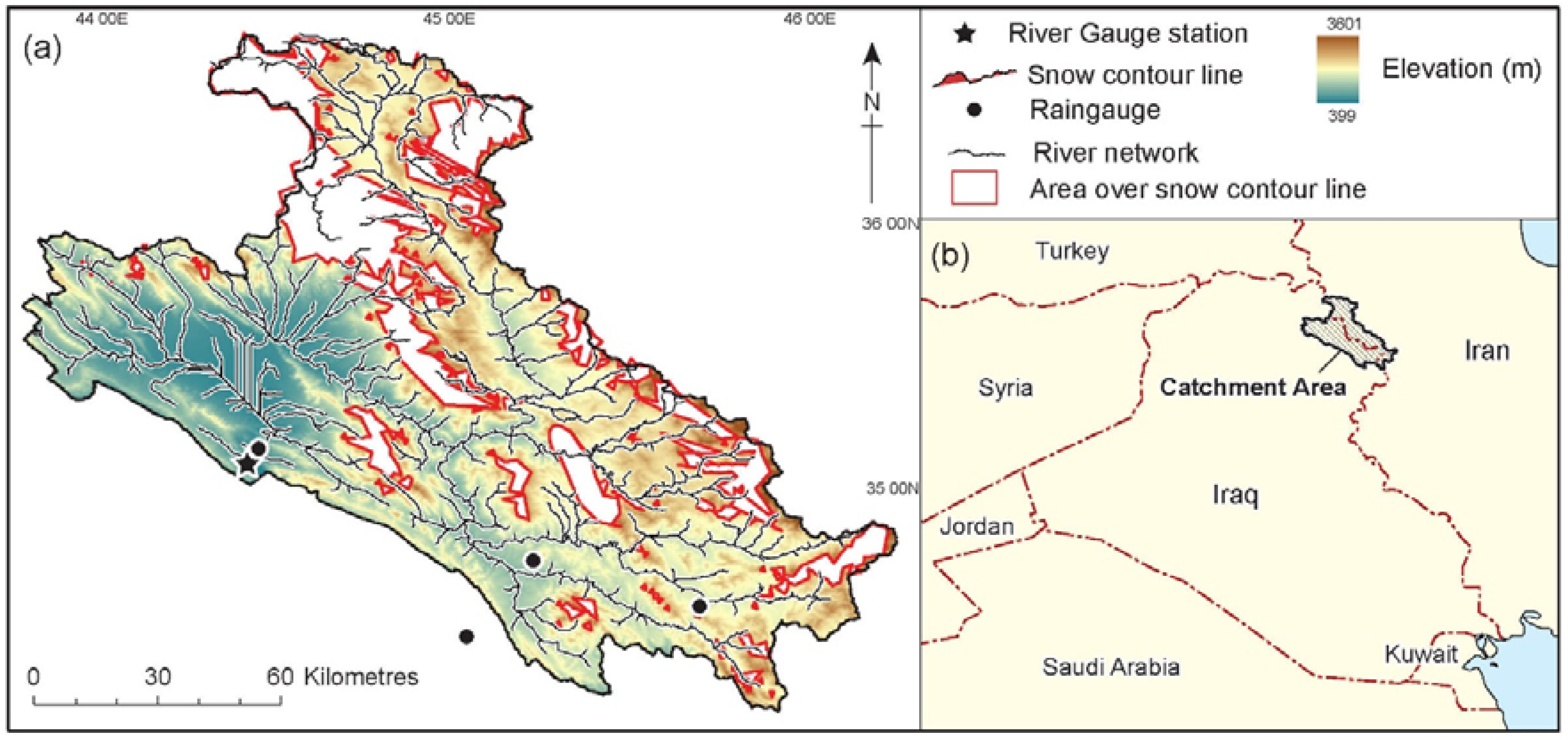
The Lesser Zab is one of the main tributaries of the river Tigris. It is situated in the Kurdistan region of northeastern Iraq (35°49′14″ N, 44°51′39″ E to 36°12′03″ N, 46°28′48″ E: Figure 1). The catchment boundary was delineated using 30 m resolution digital elevation data from the Shuttle Radar Topography Mission (SRTM).
The catchment is bounded by the Zagros Mountains to the northeast, which extend across the border with Iran. The closing section of the catchment is upstream of the Dukan Dam reservoir. The upstream catchment area is approximately 11,630 km2 with altitude ranging from 400 m to 3600 m ASL. The geology of the catchment consists of limestones, sandstone and igneous formations, dominated by a karstic aquifer system [20,21]. Land cover is predominantly extensive grazing of sparsely vegetated areas but also includes some irrigated and rain-fed arable land, woodland, open water and some small urban areas [22]. The climate of the study area is classified as subtropical semi-arid [23] which is hot and dry in summer and cool and wet in winter [24]. Precipitation mostly falls as rain in winter with mean annual precipitation ranging from 350 to >1000 mm but winter snowfall is common at elevations above 1000 m above sea level [25]. The typical mean snow line in winter is 1270 m ASL (Figure 1, [21]) which covers approximately 20% of the total catchment area. Average monthly rainfall, temperature and reference evapotranspiration rates are shown in Figure S1 of the Supplementary Material.
2.2. Data Acquisition
Meteorological data were obtained for four stations in or close to the catchment from Sulaimani Meteorological Office. These data all have daily temporal resolution from 2003 to 2014 and include maximum, minimum and average air temperature (°C), relative humidity (%), sunshine hours, wind speed (m s−1) and rainfall (mm d−1). Mean daily river discharge data for the Lesser Zab River from 2010 to 2014 were obtained from the Ministry of Agriculture and Water Resources in the Kurdistan Regional Government.
2.3. TRMM Data
The rainfall-runoff model employed here has a daily time step. Due to their high spatio-temporal resolution, the TMPA- 3B42 v7 and 3B42RT data products daily temporal resolution and 0.25° [approx. 27.83 km] spatial resolution, with global coverage from 50° N to 50° S: [daily temporal resolution and 0.25° [approx. 27.83 km] spatial resolution, with global coverage from 50°N to 50°S: 10] were selected for evaluation as suitable drivers for the model. These data were downloaded from the NASA data server (disc.sci.gsfc.nasa.gov) for the period 2003–2014. Files were processed to extract data for the catchment using R [26] and ArcGIS (ESRI, Redlands, CA, USA).
2.4. TRMM Correction
Comparisons between TRMM-derived rainfall estimates and ground-level gauge data suggest that TRMM data can sometimes be biased systematically [27]. Several attempts have been made to correct these estimates. Examples include mean bias correction [28], which uses the average bias for all stations to correct the satellite-derived rainfall, regression analysis [29] based on historical time series and the spatial bias approach [30].
Here, a bias-correction approach (originally developed for downscaling climate model outputs) was used to adjust TRMM data, based on the assumption that the satellite and in situ data have similar statistical properties [31]:
where and are the corrected and uncorrected satellite-derived rainfall estimates, respectively, is the average observed rainfall for all reporting stations, is the average satellite-derived rainfall, is the standard deviation of the observed data and is the standard deviation of satellite-derived rainfall.
This can be re-written as
where
and
Rainfall data were split into two periods: Period 1 from 2003 to 2009 (calendar years), in which we derived the two correction factors ( and ) and Period 2 from 2010 to 2014, in which the satellite-derived rainfall data were adjusted using the correction factors derived in Period 1 ( = 1.05 and = 1.24). Period 2 represents an independent validation period for the rainfall correction method.
2.5. Rainfall-Runoff Model
LEMSAR (Leicester Model for Semi-Arid Regions) is a conceptual lumped rainfall-runoff model that simulates daily river discharge using daily rainfall and potential evapotranspiration data. It is based on the models described by Whelan and Gandolfi [32] and Pullan, et al. [33], with added routines for snow melt and groundwater storage (Figure S2).
Briefly, the catchment is conceptualised using three moisture stores: (1) a single soil store, characterised by its depth (z), whole profile porosity () and by hydraulic parameters which describe the relationship between soil water content and unsaturated hydraulic conductivity; (2) a groundwater store which is augmented by recharge from the soil and depleted by baseflow to the river and (3) a time-variable snowpack.
A simple water balance is considered for the soil store:
where is the whole profile soil water storage (mm), is time (d), P is precipitation as rainfall (mm d−1), ET is actual evapotranspiration (mm d−1), is overland flow (mm d−1), q is vertical drainage out of the soil (mm d−1) and is the area-weighted input from snowmelt (mm d−1).
Actual evapotranspiration is calculated from reference evapotranspiration (ETₒ) which can be either be imported or calculated from temperature using the Hargreaves equation [34]. It is assumed that ET is equal to ETₒ when the soil moisture content exceeds a threshold value, θT, and that there is a linear decrease in ET as soil moisture content is depleted below θT down to zero at the permanent wilting point (θR). In the work described in this paper ETₒ was assumed to be equivalent to the reference ET rate which was imported from the Wasim-ET model [35] employing the FAO Penman-Monteith equation.
In the absence of a snow pack, Hortonian overland flow is described after Kirkby, et al. [36] using:
where is a constant runoff threshold for precipitation (mm d−1) and is a dimensionless proportion of excess rainfall that flows over the land surface. Note that when P < R0, is zero.
Vertical drainage out of the soil is calculated using a simple gravity flow approximation under unit hydraulic gradient [32]:
where is the unsaturated hydraulic conductivity (mm d−1) at average profile volumetric water content (θ, cm3 cm −3). The daily value of q is partitioned between direct transfer to surface water (e.g., via shallow throughflow: qTF) and groundwater recharge (qGW) using an empirically-derived (calibrated) partition factor ranging between 0 and 1:
is calculated using the Mualem-van Genuchten equation [37]:
where is the saturated hydraulic conductivity (mm d−1), is an empirical shape factor parameter of the soil water retention curve and is the dimensionless water content (0 to 1):
where is the average profile residual water content (cm3 cm−3), assumed here to be the storage at the permanent wilting point—i.e., the water content at −1500 kPa tension). Note that in the Mualem-van Genuchten model is often lower than the wilting point but here the equations are employed with different physical significance for the parameters, which represent effective area responses rather than describing hydraulic properties at the Darcy scale [33].
The shape parameter m is related to the van Genuchten parameter n via:
Snow accumulation and snow melt are assumed to occur in limited zones of the catchment delineated by altitude using the SRTM 30 m DEM. The daily air temperature in each zone is estimated from reference weather station data via:
where is the temperature of zone i, is the dry adiabatic lapse rate (0.0065 °C m−1: [38], is the mean elevation of zone i (m) and is the elevation of the nearest reference station (m).
The treatment of the snowpack is based on a simple mass balance algorithm of water equivalent units similar to that employed in the HBV model [39] which is augmented by snowfall and depleted by snowmelt. All precipitation in a zone is assumed to fall as snow when the daily average temperature () for the zone is below −0.5 °C [40]. When the zonal temperature is above 1.5 °C all precipitation is assumed to be rainfall and between −0.5 and 1.5 °C the fraction of precipitation assumed to fall as snow is calculated by linear interpolation. Snow melt is assumed to be independent of the size of the snow store (except when the snow pack is exhausted) and is calculated from the difference between mean air temperate and 0 °C multiplied by a degree-day factor [41]. Although simplistic, this approach has been shown to produce reasonable results [42,43]. The daily rate of melting in each zone () is given by:
where is degree-day factor ranging between 2 and 2.5 (mm °C−1d−1), is conversion factor for energy flux density to snowmelt depth (set to 0.26) [41], is a threshold temperature below which no melting occurs and is the net radiation flux density in water equivalent units (mm d−1). Rn is calculated from sunshine hours at the reference meteorological stations using the Angstrom formula and assuming a snow albedo of 0.7 [44]. No adjustments for changes in cloud cover with altitude are made. Total snow melt Mtot is the area-weighted average of the daily snow melt in each zone which is added to the main soil store.
Baseflow is assumed to be proportional to water storage (SG) in groundwater via a non-linear storage model [45]:
where is groundwater discharge (mm d−1) and (>0) and typically 0–1: [46] are empirical coefficients. is derived from mass balance as:
The predicted total daily river discharge (: mm d−1) is calculated as
2.6. Calibration and Validation of the LEMSAR Model
The observed discharge data were divided into two subsets, one for calibration and the another for validation. Calibration was performed using the Self Organizing Migrating Algorithm [47]. The Nash-Sutcliffe Efficiency [48] was adopted as the objective function. Optimal parameter values are shown in Table 1 along with the range within which the parameters values were constrained in the SOMA procedure. The initial value for S was also optimised in the calibration routine but the initial value for SG was arbitrarily set to 100 mm. Various configurations of the groundwater parameterization were attempted. Optimizing in the SOMA procedure ( = 0.72) gave a NSE of 0.75 and Bias = 1.1% and a reasonable prediction of base flow. However, the slope of the 1:1 line in this calibration was closer to 1 when was arbitrarily set to 1 (i.e., when groundwater is represented by a linear reservoir), the NSE was unaffected although the Bias was higher (−12.6%). Furthermore, model performance in the validation period was superior when was fixed at 1 (Bias = 4%). Given the considerable uncertainty in the behaviour of the groundwater store in this catchment we, therefore, chose to fix = 1 in all subsequent simulations. This issue is discussed further below. Four statistical measures were used to evaluate model performance in validation: the NSE; Pearson’s Correlation Coefficient (r); the root-mean-square error (RMSE) and Percent bias (see Equations (S4)–(S7) of the Supplementary Material). The model was validated three times (using a different rainfall data set in each case) in order to evalute the value of satellite-derived rainfall as the driver for predicted runoff in this catchment and, potentially, in large semi-arid data-poor catchments.
2.7. Equifinality and Sensitivity Analysis in LEMSAR
Uncertainty analysis was conducted using the Generalised Likelihood Uncertinty Estimation (GLUE) methodology [49]. R code for GLUE was obtained from a link in [50] and incorporated into the LEMSAR model. Briefly, a Monte Carlo Simulation (MCS) is performed in which model parameters are selected randomly from uniform distributions with pre-defined ranges in a large number of iterations. Model performance is estimated using a likelihood function (0–1) which is zero for parameter combinations which do not reflect system behaviour and unity for “optimal” parameter combinations. GLUE can help to identify equifinality—the existence of different combinations of parameters which generate similarly “good” representations of system behaviour [51]. This often occurs when models are poorly constrained (e.g., they are evaluated solely on the basis of one predictor, such as stream discharge, with no check on model performance with respect to other predicted state variables, such as soil water content or groundwater storage). Here, 10,000 model iterations were performed and the NSE (Equation (S4)) for Q (Equation (17)) was used as the likelihood function. An acceptability threshold of 0.5 was selected for NSE based on the model performance classification executed by Moriasi, et al. [52], (i.e., simulations were considered to be acceptable for NSE > 0.5).
3. Results
3.1. Comparison Between Gauged Rainfall and TRMM Data
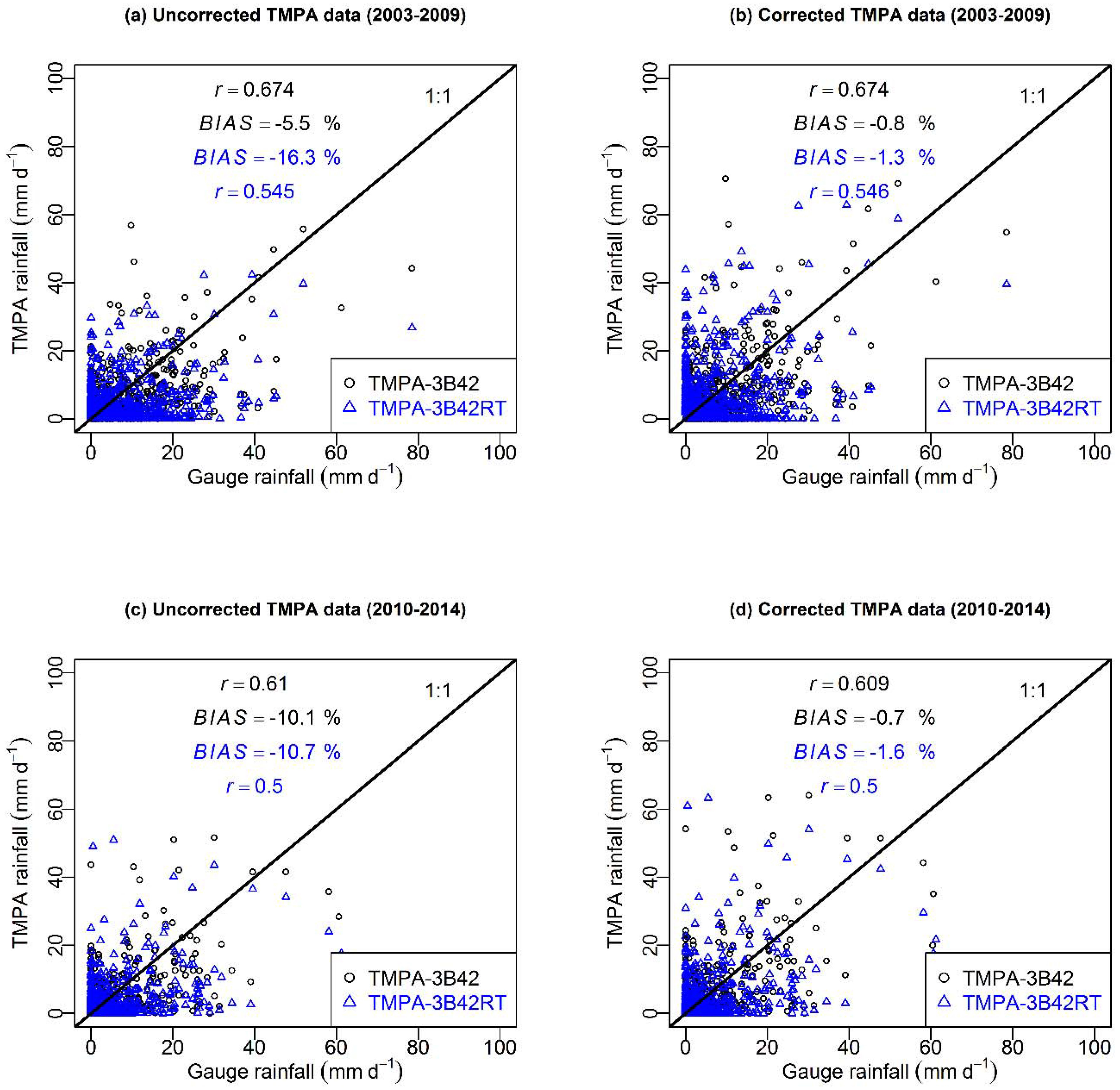
Weighted-mean (Thiessen polygon) daily ground-observed rainfall is plotted against both uncorrected and corrected TMPA-3B42/3B42RT data for Periods 1 and 2 in Figure 2. Correlation coefficients (r) were highly significant in both cases (p < 0.0001) but there is a lot of scatter around the 1:1 line and, in general, the satellite-derived data tended to under-estimate the gauged data (negative bias). Figure 2 shows that for Period 1 the correction of the TMPA-3B42 and TMPA-3B42RT data resulted in a slight change to r (from 0.674 to 0.673 and from 0.545 to 0.546, respectively) but also a decrease in the magnitude of the bias (from −5.5% to −0.8% and −16.3% to −1.3%, respectively). For Period 2 (Figure 2c,d) the application of the correction factors derived with the Period 1 data also resulted in little change to r but reduced the bias from −10% to −0.7% for TMPA-3B42 and from −10.7% to −1.6% for TMPA-3B42RT.
To further investigate the correspondence between TMPA-3B42/3B42RT estimates and the rain gauge data, we also employed the following verification metrics, based on a contingency table (Table S1): (i) the False Alarm Ratio (FAR) i.e., the ratio of the number of times rainfall was forecast by the satellite data product but not observed in the gauged rainfall data to the total number of times rain was forecasted successfully (see Equation (S1)); (ii) the Probability of Detection (POD; see Equation (S2)) i.e., the ratio of the number of times rain days were successfully forecasted to the total number of rain days [53,54]) and (iii) the Heidke Skill Score (HSS; see Equation (S3)) i.e., a measure of the frequency of correct matches between satellite forecasts and gauged observations compared to the number of correct matches which would be expected by chance [53,55]. These verification statistics for Periods 1 and 2 are displayed in Figure S3. The FAR values for both the uncorrected and corrected TMPA-3B42RT were higher than those calculated for TMPA-3B42 for both Periods 1 and 2. The POD values were lower for the TMPA-3B42RT data than for the TMPA-3B42 for both periods. Overall, the 3B42 data performed better than the 3B42RT data. However, these statistics show that both TMPA products have serious problems in detecting the occurrence or not of rainfall. Values of HSS were about 0.4 for Period 1 and 0.3 for Period 2 for most rainfall intensities. Note that positive values of HSS indicate that the TMPA data products were better than chance. This is the case for the most common rainfall intensities (i.e., between 5 and 45 mm d−1).
3.2. Comparing Observed and Simulated Discharge
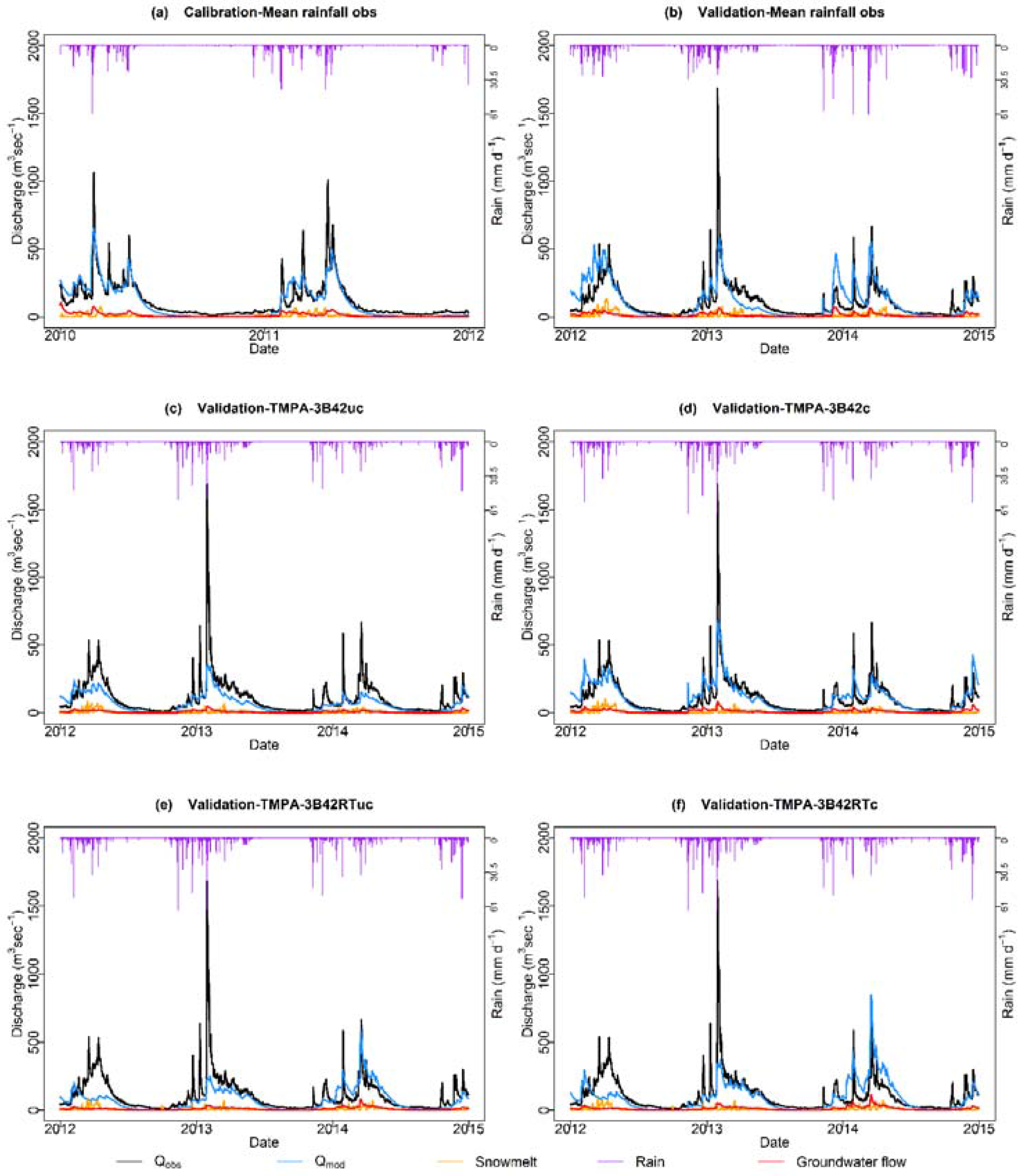
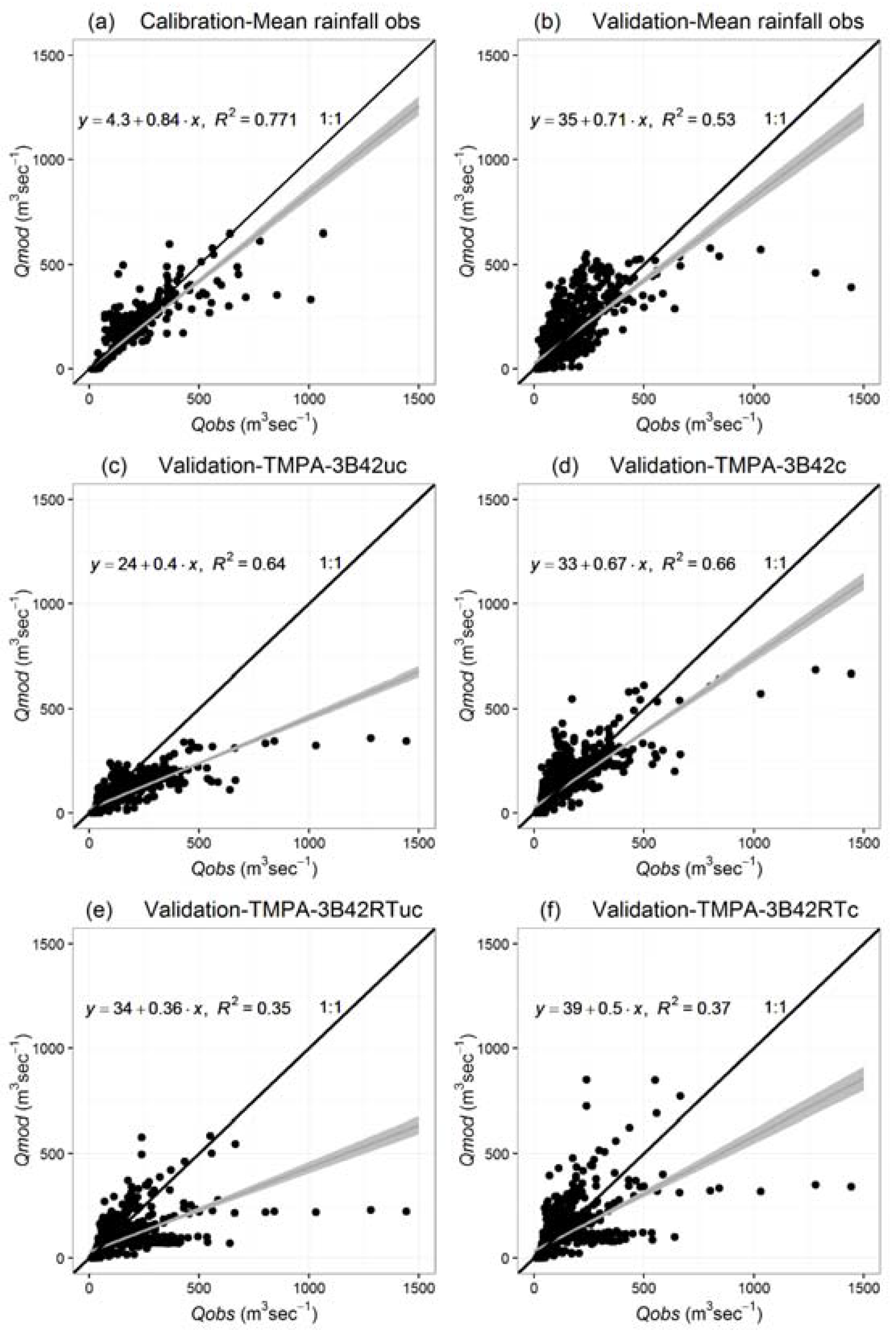
Observed and simulated discharge for the Lesser Zab River in different periods and driven by different rainfall data sets are shown in Figure 3. In all cases, the black line shows the observed discharge, the orange line represents predicted snowmelt and the red line is groundwater flow. In general, the seasonal agreement between observed and simulated discharge is reasonable using both gauge-derived and corrected TMPA-3B42/3B42RT rainfall data. However, some hydrograph peaks appear to be noticeably under-predicted by the model, particularly when driven by the uncorrected TMPA-3B42/3B42RT rainfall data. In part, this reflects a general tendency for the TMPA data to under-estimate the gauge-derived rainfall data. Simulated flows are plotted against measured data in Figure 4, along with the best-fit linear regression and the 1:1 line. Most of the points are scattered around the 1:1 line when the model is driven by the area-weighted rain gauge data. However, there is considerable deviation at high flows (e.g., the model underestimates some measured discharge peaks >500 m3s−1) and for hydrograph recessions (in which predicted flows tend to reduce slightly faster than those observed). This results in a slope for the best-fit regression which is less than unity in the validation period. This systematic deviation was more pronounced when the model was driven by the uncorrected TMPA-3B42 and TMPA-3BRT rainfall data (Figure 4c,e). However, the TMPA correction procedure noticeably reduced (but did not eliminate) the systematic tendency for the model to under-estimate measured flow and resulted in tolerable discharge predictions overall. It is important to note that the factors ( and ) used for the correction of the TMPA data were derived from Period 1 (2003–2009) which does not overlap with either the calibration or the validation periods used for evaluating the hydrological model. The TMPA corrections are, therefore, independent of the rain gauge data used to drive the hydrological model over 2010–2014. Statistical comparisons between simulated and measured flows are also plotted on Taylor Diagrams in Figure S4. These diagrams summarise the overall performance of LEMSAR during the calibration and validation periods when driven by different precipitation data.
Goodness-of-fit statistics are presented in Table 2. These statistics reinforce the message derived from the graphs that the model tends to under-estimate the measured river discharge in both the calibration and validation periods regardless of the rainfall data used. The bias was lowest when the measured rainfall data were used to drive the model and highest when the uncorrected TMPA-3B42/3B42RT rainfall data were used. However, the best NSE value for the validation period was obtained using the corrected TMPA-3B42 data. As expected, model performance was poorest when it was driven by the uncorrected TMPA-3B42/3B42RT data (lowest NSE, highest BIAS and highest RMSE). Overall, using the TMPA-3B42 product resulted in better model performance compared to usingTMPA-3B42RT product.
3.3. Contribution of Snowmelt and Groundwater Flow to Simulated River Discharge
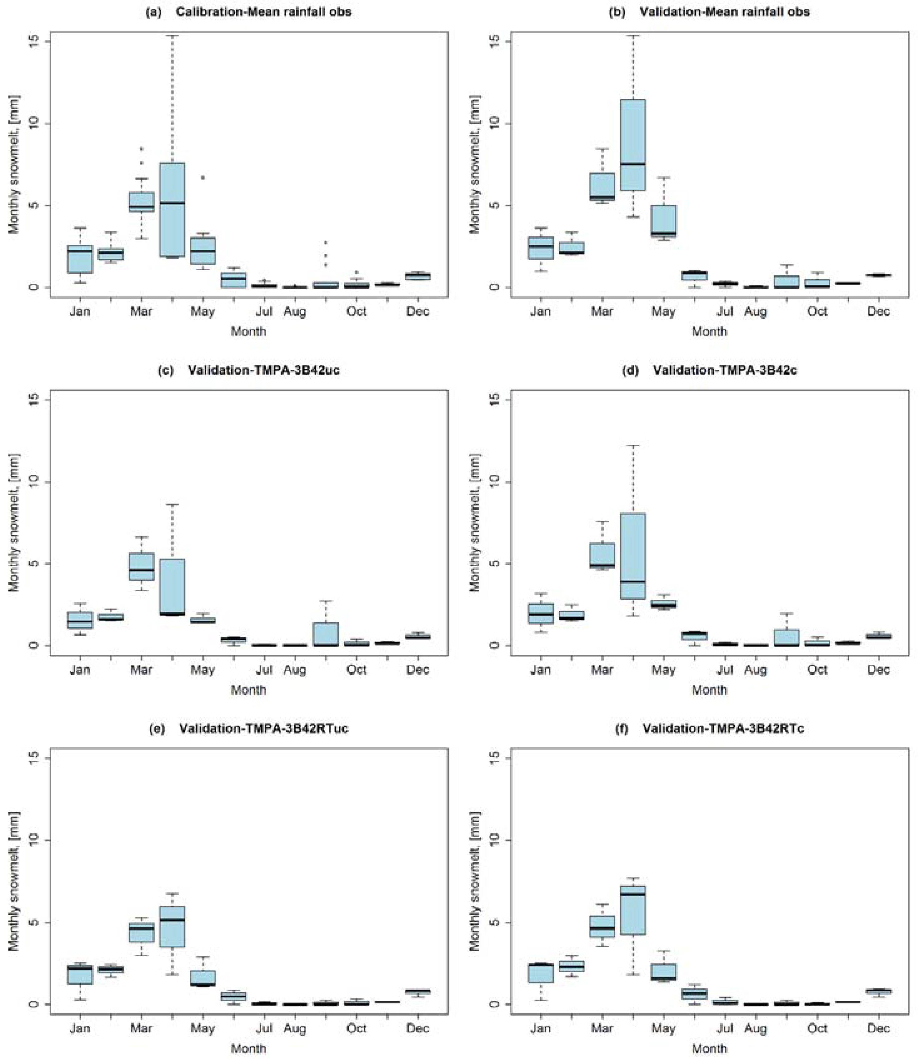
The daily predicted contributions of snowmelt and groundwater in the Lesser Zab catchment are shown in (Figure 3). Although predicted daily snow melt contributions to total flow tended to be low (annual percentage contribution 4%–13.5%), predicted melt-derived flows can be substantial in spring and may contribute to occasional flood events (Figure 5). Monthly snowmelt contributions were highest when the model was driven by gauged rainfall data, principally due to a higher winter precipitation rate observed compared to both the uncorrected and corrected TMPA products, and hence a deeper simulated snowpack accumulation. The snowmelt contributions were also higher when LEMSAR was driven by both uncorrected and corrected TMPA-3B42RT data than it was driven by the TMPA-3B42 data.
The predicted contribution of groundwater flow to river discharge is low and significantly underestimates baseflow. This is, in part, due to the simplistic representation of the complex and highly uncertain hydrogeological system underlying this catchment but it is also a result of the model parameterisation (including our arbitrary decision to set = 1). Overall model performance tended to be better with a high value of k (implying very steep groundwater recession and a perenially low groundwater storage). Many of the underlying strata in the catchment are karstic (i.e., they contain a highly conductive network of cracks and fissures) which respond rapidly during storm events but which have baseflow behaviours which are difficult to model [56]. A high value of k is consistent with the rapid behaviour of karstic systems, although we recognise that it penalises model performance at low flows in order to get a better simulation of the hydrograph during storm events.
3.4. Flow Duration Curves
Flow duration curves (FDC) for both observed and simulated river discharge are shown in Figure 6. The match between the curves is generally good, although there is some under-prediction of discharge at high exceedance percentiles (i.e., low flows tend to be under predicted) and some over-prediction of flows in the 5–25 exceedance percentile range. Again, the under-prediction of low flows is due in part to the simple nature of the baseflow model adopted here and its parameterisation. The source of rainfall data used to drive the model had a significant effect on the shape of the FDC. Flows were under predicted over most of the range when the model was driven by the uncorrected TMPA-3B42 and 3B42RT data but this noticeably improved for a significant percentile range when the TMPA-3B42/3B42RT data were corrected. Overall, reproduction of the FDC was slightly better when the model was driven by the corrected TMPA-3B42RT data than when it was driven by the TMPA-3B42 data.
3.5. Equifinality
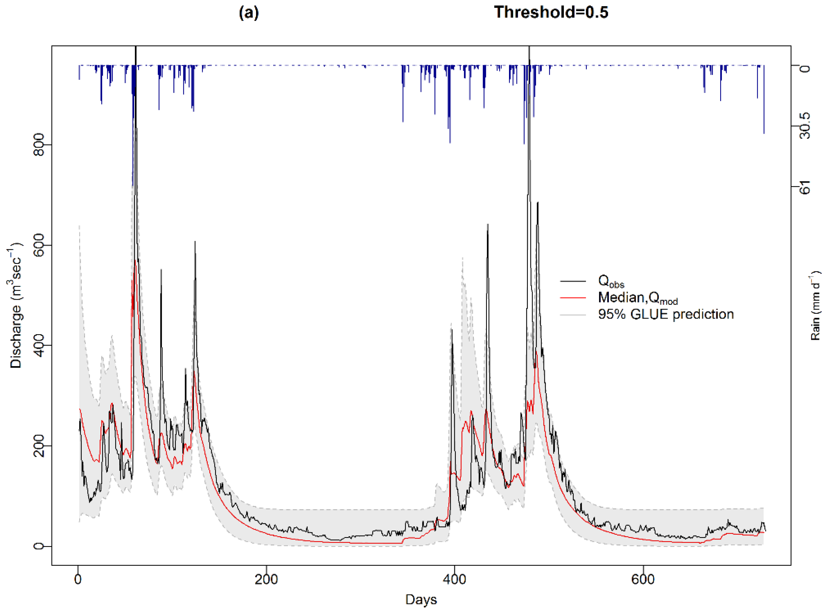
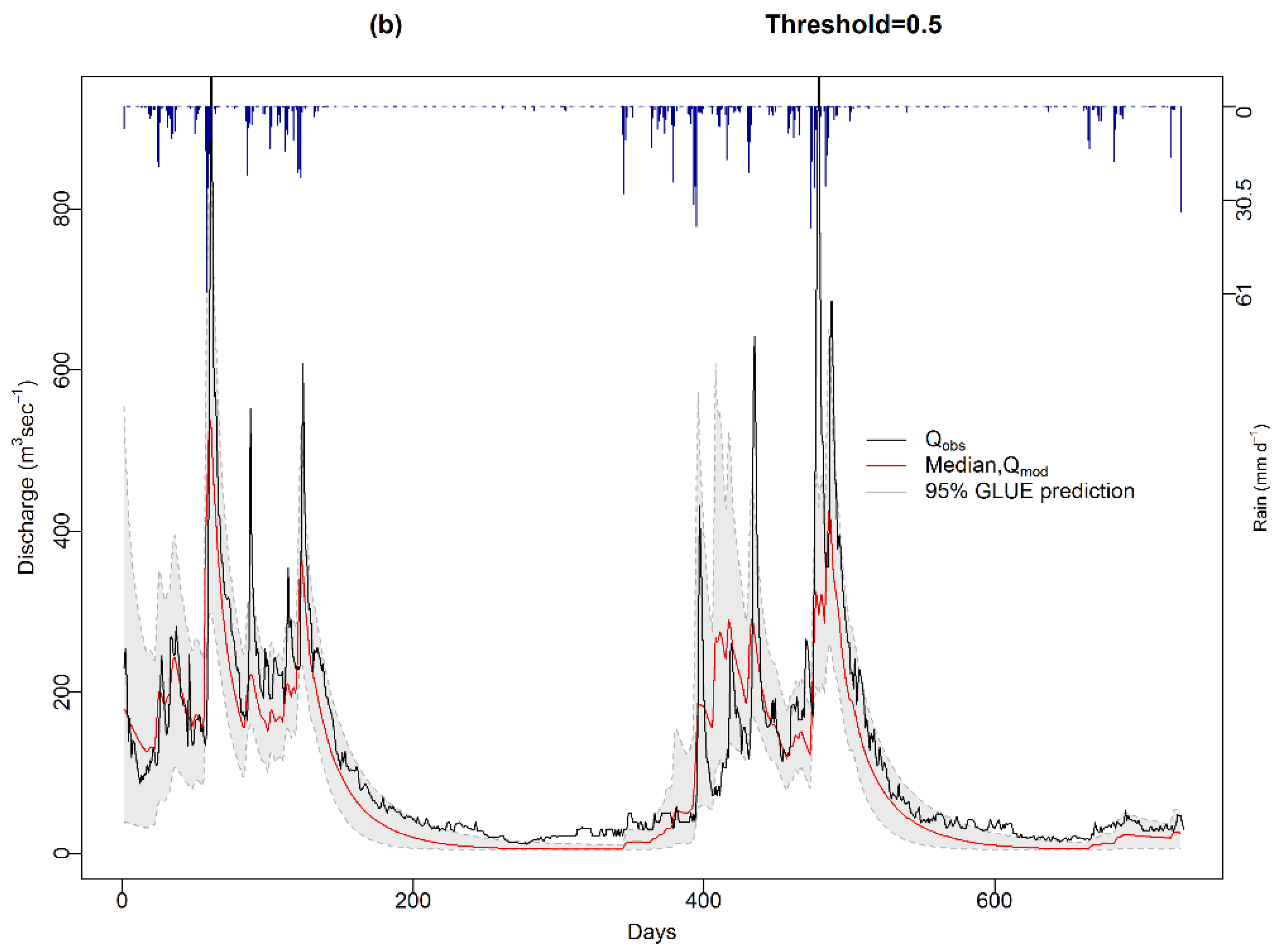
Figure 7 shows scatter plots of NSE against MCS-generated parameter values for the calibration period. The blue point indicates the NSE for the calibrated (reference) parameter set (NSE = 0.75). Only parameter combinations yielding NSE > 0.5, are displayed. The graphs clearly demonstrate the frequently reported phenomenon of equifinality [7,49,57,58,59,60] in which reasonable model performance can be achieved using several different combinations of model parameters. Here it occurs, in part, due to the fact that our model is poorly constrained (i.e., measured data are available for only one predicted output variable—stream discharge, with other predicted internal state variables, such as soil water content and groundwater storage, not measured and, hence, not validated). Hence, the “optimal” set of model parameters yields good predictions of the data available but may actually produce poor simulations for unmeasured phenomena such as snow melt and baseflow contributions (i.e., the model may give the “right results for the wrong reasons”). Although it is possible to apply qualitative constraints on parameter combinations to ensure that unmeasured state variable predictions are “sensible” [61], the lack of measured data for these variables mean that both aleatory and epistemic uncertainty are always high. Equifinality also makes evaluating the relative contributions of errors in the individual terms of the water balance equations to the overall model error difficult if not impossible. This is in part, because many of these terms are linked e.g., via a dependence on soil moisture or contain parameters which are calibrated on discharge at the catchment outlet, rather than being determined independently. The results from a local sensitivity analysis are presented in the Supplementary Material (see Figure S5) and suggest the following rank order for model sensitivity (high to low > n > z > Ksat > fg> θT, θR, θr, p, Ro, k. Given the relative insenstitivity of the model performance to θT, θR, θr, p, Ro, and k these parameters were fixed to their optimal values and the MCS re-run to generate GLUE uncertainty boundaries on predicted discharge. These are shown in Figure 8 for the calibration period (2010–2011).
4. Discussion
In this paper, we present a simple rainfall-runoff model which we apply, for the first time, to the Lesser Zab catchment in Iraq using weighted average gauged daily rainfall data and rainfall data derived from remote sensing. The principal aim was to assess the potential value of remotely-sensed rainfall data as a driver for rainfall-runoff modelling in data-scarce semi-arid catchments. Although data availability for the Lesser Zab catchment was actually sufficient for hydrological modelling, this is atypical of most semi-arid regions in the world which often suffer from data scarcity issues related to inadequate resource allocation for instrumentation and monitoring [62]. Moreover, even when data exist, they may not be made available for scientific studies without appropriate connections to the data-holding authorities. This study, therefore, provides an excellent opportunity to evaluate model performance and the utility of remotely sensed data under various assumptions of data paucity.
Two daily satellite-derived data products (TMPA-3B42 and 3B42RT) were corrected using mean bias statistics (mean and standard deviation) assuming uniform bias across the whole range of rainfall intensities. Five river discharge simulations were performed, driven by different daily rainfall data sets (gauged data, uncorrected TMPA3B42 data, uncorrected TMPA-3B42RT data, corrected TMPA-3B42 and corrected TMPA-3B42RT data). Both the uncorrected TMPA data products tended to underestimate gauge-derived rainfall. The performance of the TMPA-3B42RT product was poorer than that of the TMPA-3B42 product during rainy days. The 3B42RT also had a higher tendency to predict rainfall on days in which there was no gauge-observed rainfall (hence the higher FAR). In addition, the TMPA-3B42 data generated higher POD values than the 3B42RT data, confirming better performance for predicting rainy days. Generally, the HSS of both products was best for rainfall rates between 5 and 45 mm d−1. Failure to accurately predict events with higher intensities could be related to the low spatial and temporal resolution of the TMPA data products (the time interval between TRMM orbits is too long to capture all rainfall events [30] and the random, short duration and localized nature of high intensity convective storm events in arid and semi-arid areas which contribute to greater spatial variability for precipitation in these areas compared with humid regions [63]. This is also an issue for precipitation capture by rain gauges, especially if they are sparsely located [64]. That said, overall trends are generally captured well.
Aside from the localised nature of convective rainfall, there are many possible explanations for deviations of the TMPA rainfall from the gauge-recorded data, including the influence of topography (e.g., slope, aspect and local relief) [65]. In addition, known (and unknown) instrument errors (e.g., the TRMM radar cannot detect rainfall at less than about ~18 dBZ or 0.4 mm/h [66]) will also contribute to deviations. We used area-averaged (Thiessen polygon weighted averaging) precipitation measurements derived from ground observations from four stations over a limited period to correct the TMPA data. These data are associated with considerable uncertainty due to instrument and sampling errors arising from the relatively low spatial density of gauges. In particular, these stations are predominantly located at low elevations (550 to 1300 m ASL) and, hence may under-estimate total precipitation at altitude and total catchment precipitation in general. However, data to verify the extent to which this may have been a major issue or not are currently not available. The uncorrected and corrected TMPA-3B42 data both underestimated gauged data by −10% and −0.7% respectively. Similarly, the TMPA-3B42RT underestimated gauged data by −10.7% and −1.3 respectively. This finding is in rough agreement with [67] which reported that satellite-derived rainfall could systematically underestimate ground observed rainfall by 30% or more. Collischonn, Collischonn and Tucci [4] also showed that relative differences between observed and satellite-derived rainfall data can range from −39% to +25%.
Given the simplicity of the model assumptions and the large and complex nature of the catchment, the performance of the LEMSAR model in the Lesser Zab catchment was surprisingly good. Although model performance was weak in places (e.g., the poor prediction of baseflow), performance overall was equivalent or better than that obtained using similar model in smaller UK catchments [33]. The contribution of snow melt and baseflow to river discharge is unknown and the model is poorly constrained with respect to these simulations. This contributed to significant equifinality, illustrated by a wide range of “acceptable” parameter combinations. Although a significant part of the catchment is above 1500 m altitude and, therefore, likely to receive some winter precipitation as snow, the relative contribution of calculated snowmelt to simulated river discharge was generally low, even in the spring melt season (although the absolute volumes were occasionally significant and the snow melt contribution may have been masked by coincidentally high rainfall in this season). However, it would be useful to confirm this prediction by independent studies in high altitude sub-catchments.
No adjustment was made in the model for changes in ETₒ with altitude or over snow cover. Instead a weighted average daily ETₒ value from the available meteorological stations was used to drive the model. Since ETₒ is likely to decrease with altitude, this assumption is likely to lead to an overestimation in mean catchment ETₒ. Estimated evapotranspiration and sublimation from snow and frozen soil has generally been reported to be low [68]. For example, Male and Granger [69] estimated daily net evaporation rates of 0.02–0.3 mm d−1 in central Saskatchewan. However, in any case, snow cover is predicted to occur in a maximum of 20% of the catchment area and only for three months of the year. Given the lumped nature of the model employed and the other major simplifications assumed, therefore, we expect the impact of this uncertainty is relatively minor.
The behaviour of the regional groundwater system in our model was simplistic, reflecting high epistemic uncertainty. In fact, model performance was highest overall when was fixed at 1 and k was high (resulting in minimal groundwater contribution), suggesting that the aquifer reacts like a single linear reservoir where the groundwater flow is proportional to groundwater storage and water release from the soil store is the principal limit on the timing and magnitude of river discharge. This will, in turn, be controlled by seasonal changes in evapotranspiration and soil moisture content, similar to many humid-temperate catchments. Although the dominant underlying karstic strata in the catchment are volumetrically important, they have rapid hydrological response times [56]. We can postulate, therefore, that delays in groundwater flow are short and make little modification to hydrograph shape and magnitude. However, one important issue with this assumption is that low flows in the sustained dry summers experienced in the catchment are poorly predicted. This is clearly important from a water resources management perspective but does not affect the evaluation of the TMPA-3B42/3B42RTdata as a driver for hydrological modelling. Resolving this issue is, therefore, beyond the scope of this paper but one solution could be to simply assume an additional fixed baseflow. Finally, although there will be channel network delays in the translation of rainfall to runoff in such a large catchment (>11,000 km2), these delays are not likely to be important at the daily time step (i.e., network travel times will still be mostly < 24 h—particularly during storm events). Although some modelling uncertainty could be reduced by excluding model-insensitive parameters from the [51], constraining simulations using measured state variables such as soil water content, snow melt and groundwater behaviour would clearly be more beneficial [70,71,72].
Observed discharge in the Lesser Zab river was represented reasonably well by the model using in situ gauged rainfall and both TMPA-3B42 and 3B42RT data, particularly when the latter were corrected using a limited set of rain gauge data. Flow simulations using uncorrected TMPA-3B42/3B42RT data generally under-estimated flows for significant periods, with some peaks missed altogether, although seasonal fluctuations were still well captured. It has been reported that TMPA bias tends to increase with rainfall intensity [73], suggesting that the bias is multiplicative, not additive. In our study, some rainfall events >40 mm d−1 do appear to become more biased after correction (Figure 2b). This means that although our corrections improve rainfall over the most frequent ranges (typically low intensity), they may fail to improve significantly (or worsen) model performance in lower frequency, higher magnitude events. Application of different bias statistics for different ranges of rainfall intensity could provide a solution to this issue but this has not been explored further here.
The superior accuracy of LEMSAR when driven by corrected, compared to uncorrected, TRMM data mainly reflects the fact that the correction reduced the bias in the TRMM estimates which was translated, in part, into higher predicted flows. These results are consistent with other research [4,74,75] which has indicated that corrected TMPA-3B42 v7 precipitation estimates can provide reasonable model input for the simulation of discharge river. However, previous attempts at correction have used denser rain gauge networks than the network employed here and none have been employed in this region. The TMPA-3B42/3B42RT data were corrected using a limited set of the available rain gauge data in order to evaluate the application of the correction equation to independent data. The agreement between the corrected daily TMPA-3B42/3B42RT data and the daily rain gauge data for Period 2, together with the reasonable performance of LEMSAR when driven by the corrected TMPA data for the whole flow record, suggest that this correction may be generally applicable in this catchment. Nevertheless, it should be noted that the superior performance of the model when driven by both of the corrected satellite data products may be “opportunistic” to some extent—resulting from the fact that flows are slightly over-estimated by the model when calibrated using gauged rainfall whilst gauged rainfall is still slightly under-estimated by the TMPA data.
Furthermore, since the TMPA data provide spatially aggregated rainfall estimates over an area, while rain gauge data are measured at specific point locations, the TMPA data may be useful for modelling catchments where gauge data are sparse. Note that the TRMM data mission has now ended and another platform (Global Precipitation Measurement (GPM) mission is available at http://pmm.nasa.gov/GPM) which supplies similar data to TRMM. The Integrated Multi-satellitE Retrievals for GPM (IMERG) will be much improved in terms of spatial and temporal resolutions (e.g., 0.1 deg and half-hourly [76]). The findings of this work should also be broadly applicable to GPM data.
All hydrological model runs used weighted average values of daily ETₒ calculated from ground-based meteorological observations. Here, we have evaluated only the utility of remotely-sensed rainfall data for driving a hydrological model. Further work should also explore the effects of using other remotely sensed meteorological data (e.g., surface temperature) to predict ETₒ and the potential for simulating hydrological response in this and other catchments completely independently of ground-based observations.
5. Conclusions
Semi-arid regions often have sparse rain gauge networks. Satellite-based precipitation estimates can, therefore, potentially provide crucial information for evaluating runoff using hydrological models. In this study, we explored the utility of satellite-derived data to force a simple water balance model. We found that both data products were biased towards an under-estimation of observed rainfall in the Lesser Zab catchment and needed to be corrected. A bias-correction approach was employed, which rescales standard scores (z scores) using the mean and standard deviation of the gauged rainfall data. Overall, model performance for predicting discharge was reasonable, particularly given the relatively simplistic assumptions made and the large size of the catchment. This suggests that runoff dynamics in this catchment are principally controlled by the soil moisture balance and that groundwater dynamics and snow melt make relatively small contributions to the shape and magnitude of the hydrograph (although snow melt is predicted to be significant in spring and baseflow is important in the dry season). However, significant uncertainty exists in the model simulations reported, manifested as equifinality. The aleatory component of this uncertainty could be quantified using GLUE which defines uncertainty bounds on predicted flows (resulting, in part, from poorly constrained calibration) but epistemic uncertainty is unknown and likely to be significant. Overall the TMPA-3B42 data product out-performed the 3B42RT data in terms of POD, HSS and FAR compared with gauged rainfall. Hydrological model performance was also generally better when driven by the corrected 3B42 data than when the 3B42RT data were used. When LEMSAR was driven by corrected TMPA- 3B42c rainfall, predicted runoff in the validation period was as good as or better than that predicted using gauge-derived data. This suggests that the corrected TMPA rainfall data particularly TMPA-3B42 (or equivalent data from GPM) can be used to predict river discharge in this catchment which may be useful for future water resources management (e.g., estimating the availability of water resources in ungauged catchments and to anticipate the need for temporary controls on water use at times of water scarcity).
Supplementary Materials
The following are available online at www.mdpi.com/2225-1154/5/2/32/s1.
Acknowledgments
This research was funded via a scholarship from the Higher Committee for Education Development in Iraq (HCED) with support from the NERC National Centre for Earth Observation. We are grateful to the Hydrology Department of the Dukan Dam Directorate for providing river discharge data and to the Directorate of Meteorology in Sulaimanyiah for providing meteorological data. HB was supported by a Royal Society Wolfson Research Merit Award (2011/R3) and MW benefitted from Study Leave granted by the University of Leicester.
Author Contributions
This paper is the result of research conducted by Peshawa Najmaddin (PN) as part of his PhD studies at the University of Leicester. Mick Whelan (MW) and Heiko Balzter (HB) jointly supervised this project. Model coding was conducted by PN with guidance from MW. HB provided guidance on the analysis of the remote sensing data. The manuscript was prepared by PN with suggestions and corrections from MW and HB. All authors have seen and approved the final article.
Conflicts of Interest
The authors declare no conflict of interest. The founding sponsors had no role in the design of the study; in the collection, analyses, or interpretation of data; in the writing of the manuscript, and in the decision to publish the results.
References
- Wheater, H.S. Progress in and prospects for fluvial flood modelling. Philos. Trans. Ser. A Math. Phys. Eng. Sci. 2002, 360, 1409–1431. [Google Scholar] [CrossRef] [PubMed]
- Beaumont, P.; Blake, G.; Wagstaff, J.M. The middle East: A Geographical Study, 2nd ed.; Routledge: Oxford, UK, 2016. [Google Scholar]
- Sawunyama, T.; Hughes, D.A. Application of satellite-derived rainfall estimates to extendwater resource simulation modelling in South Africa. Pretoria Water Res. Comm. 2008, 34, 1–9. [Google Scholar]
- Collischonn, B.; Collischonn, W.; Tucci, C.E.M. Daily hydrological modeling in the amazon basin using trmm rainfall estimates. J. Hydrol. 2008, 360, 207–216. [Google Scholar] [CrossRef]
- Draper, C.S.; Walker, J.P.; Steinle, P.J.; de Jeu, R.A.M.; Holmes, T.R.H. An evaluation of AMSR–E derived soil moisture over Australia. Remote Sens. Environ. 2009, 113, 703–710. [Google Scholar] [CrossRef]
- Voss, K.A.; Famiglietti, J.S.; Lo, M.; Linage, C.; Rodell, M.; Swenson, S.C. Groundwater depletion in the middle east from grace with implications for transboundary water management in the tigris-euphrates-western iran region. Water Resour. Res. 2013, 49, 904–914. [Google Scholar] [CrossRef] [PubMed]
- Beven, K.J.; Alcock, R.E. Modelling everything everywhere: A new approach to decision-making for water management under uncertainty. Freshwater Biol. 2012, 57, 124–132. [Google Scholar] [CrossRef]
- Huffman, G.J.; Adler, R.F.; Morrissey, M.M.; Bolvin, D.T.; Curtis, S.; Joyce, R.; Mcgavock, B.; Susskind, J. Global precipitation at one-degree daily resolution from multisatellite observations. J. Hydrometeorol. 2001, 2, 36–50. [Google Scholar] [CrossRef]
- Center, E.O. Trmm Data Users Handbook; National Space Development Agency of Japan: Hiki-gun, Saitama, Japan, 2001. [Google Scholar]
- Huffman, G.J.; Bolvin, D.T.; Nelkin, E.J.; Wolff, D.B.; Adler, R.F.; Gu, G.; Hong, Y.; Bowman, K.P.; Stocker, E.F. The trmm multisatellite precipitation analysis (TMPA): Quasi-Global, multiyear, combined-sensor precipitation estimates at fine scales. J. Hydrometeorol. 2007, 8, 38–55. [Google Scholar] [CrossRef]
- McCollum, J.R.; Gruber, A.; Ba, M.B. Discrepancy between gauges and satellite estimates of rainfall in equatorial africa. J. Appl. Meteorol. 2000, 39, 666–679. [Google Scholar] [CrossRef]
- New, M.; Lister, D.; Hulme, M.; Makin, I. A highresolution data set of surface climate over global land areas. Clim. Res. 2002, 21, 1–25. [Google Scholar] [CrossRef]
- Zulkafli, Z.; Buytaert, W.; Onof, C.; Manz, B.; Tarnavsky, E.; Lavado, W.; Guyot, J.-L. A comparative performance analysis of TRMM 3B42 (TMPA) versions 6 and 7 for hydrological applications over Andean–Amazon river basins. J. Hydrometeorol. 2014, 15, 581–592. [Google Scholar] [CrossRef]
- Nerini, D.; Zulkafli, Z.; Wang, L.-P.; Onof, C.; Buytaert, W.; Lavado-Casimiro, W.; Guyot, J.-L. A comparative analysis of TRMM–rain gauge data merging techniques at the daily time scale for distributed rainfall–runoff modeling applications. J. Hydrometeorol. 2015, 16, 2153–2168. [Google Scholar] [CrossRef]
- Zubieta, R.; Getirana, A.; Espinoza, J.C.; Lavado, W. Impacts of satellite-based precipitation datasets on rainfall–runoff modeling of the Western Amazon basin of Peru and Ecuador. J. Hydrol. 2015, 528, 599–612. [Google Scholar] [CrossRef]
- Zubieta, R.; Saavedra, M.; Silva, Y.; Giráldez, L. Spatial analysis and temporal trends of daily precipitation concentration in the Mantaro River basin: Central andes of Peru. Stoch. Environ. Res. Risk Assess. 2016, 1–14. [Google Scholar] [CrossRef]
- Harris, A.; Rahman, S.; Hossain, F.; Yarborough, L.; Bagtzoglou, A.C.; Easson, G. Satellite-based flood modeling using TRMM-based rainfall products. Sensors 2007, 7, 3416–3427. [Google Scholar] [CrossRef]
- Beven, K.J.; Kirkby, M.J. A physically based, variable contributing area model of basin hydrology/Un modèle à base physique de zone d’appel variable de l’hydrologie du bassin versant. Hydrol. Sci. Bull. 1979, 24, 43–69. [Google Scholar] [CrossRef]
- Tarnavsky, E.; Mulligan, M.; Ouessar, M.; Faye, A.; Black, E. Dynamic hydrological modeling in drylands with trmm based rainfall. Remote Sens. 2013, 5, 6691–6716. [Google Scholar] [CrossRef]
- Buringh, P. Soils and Soil Conditions of Iraq; Agricultural Research and Projects; Ministry of Agriculture: Baghdad, Iraq, 1960. [Google Scholar]
- Krásný, J.; Alsam, S.; Jassim, S.Z. Hydrogeology. In Geology of Iraq, 1st ed.; Publishers Dolin: Prague, Czech Republic, 2006; pp. 251–287. [Google Scholar]
- Qader, S.H.; Dash, J.; Atkinson, P.M.; Galiano, V.R. Classification of vegetation type in Iraq using satellite-based phenological parameters. IEEE J. Sel. Top. Appl. Earth Obs. Remote Sens. 2016, 43, 1–23. [Google Scholar] [CrossRef]
- Rasul, A.; Balzter, H.; Smith, C. Diurnal and seasonal variation of surface urban cool and heat islands in the semi-arid city of Erbil, Iraq. Climate 2016, 4, 42. [Google Scholar] [CrossRef]
- Food and Agriculture Organization (FAO). Country Pasture/Forage Resource Profiles. Rome, Italy, 2011. Available online: http://www.fao.org/ag/agp/AGPC/doc/Counprof/Iraq/Iraq.html (accessed on 9 January 2016).
- Zaitchik, B.F.; Evans, J.P.; Smith, R.B. Regional impact of an elevated heat source: The zagros plateau of iran. J. Clim. 2007, 20, 4133–4146. [Google Scholar] [CrossRef]
- R Development Core Team. R: A Language and Environment for Statistical Computing; R Foundation for Statistical Computing: Vienna, Austria, 2014; Available online: http://www.R-project.org/ (accessed on 5 January 2016).
- Arias-Hidalgo, M.; Bhattacharya, B.; Mynett, A.E.; van Griensven, A. Experiences in using the TMPA-3B42R satellite data to complement rain gauge measurements in the ecuadorian coastal foothills. Hydrol. Earth Syst. Sci. 2013, 17, 2905–2915. [Google Scholar] [CrossRef]
- Seo, D.J.; Breidenbach, J.P.; Johnson, E.R. Real-time estimation of mean field bias in radar rainfall data. J. Hydrol. 1999, 223, 131–147. [Google Scholar] [CrossRef]
- Immerzeel, W.W.; Rutten, M.M.; Droogers, P. Spatial downscaling of TRMM precipitation using vegetative response on the Iberian Peninsula. Remote Sens. Environ. 2009, 113, 362–370. [Google Scholar] [CrossRef]
- Cheema, M.J.M.; Bastiaanssen, W.G.M. Local calibration of remotely sensed rainfall from the trmm satellite for different periods and spatial scales in the Indus Basin. Int. J. Remote Sens. 2012, 33, 2603–2627. [Google Scholar] [CrossRef]
- Bouwer, L.M.; Aerts, J.C.J.H.; van de Coterlet, G.M.; van Giesen, N.; Gieske, A.; Manaerts, C. Evaluating downscaling methods for preparing global circulation model (GCM) data for hydrological impact modelling. In Climate Change in Contrasting River Basins: Adaptation Strategies for Water, Food and Environment; Aerts, J.C.J.H., Droogers, P., Eds.; Cabi Press: Wallingford, UK, 2004; Chapter 2; pp. 25–47. [Google Scholar]
- Whelan, M.J.; Gandolfi, C. Modelling of spatial controls on denitrification at the landscape scale. Hydrol. Process. 2002, 16, 1437–1450. [Google Scholar] [CrossRef]
- Pullan, S.P.; Whelan, M.J.; Rettino, J.; Filby, K.; Eyre, S.; Holman, I.P. Development and application of a catchment scale pesticide fate and transport model for use in drinking water risk assessment. Sci. Total Environ. 2016, 563–564, 434–447. [Google Scholar] [CrossRef] [PubMed]
- Hargreaves, G.H.; Samani, Z. Reference crop evapotranspiration from ambient air temperature. Am. Soc. Agric. Eng. 1985. [Google Scholar] [CrossRef]
- Hess, T.; Harrison, P.; Counsell, C. Wasim Technical Manual; HR Wallingford: Wallingford, UK; Cranfield University: Cranfield, UK, 2000. [Google Scholar]
- Kirkby, M.J.; Irvine, B.J.; Jones, R.J.A.; Govers, G. The pesera coarse scale erosion model for Europe. I.—Model rationale and implementation. Eur. J. Soil Sci. 2008, 59, 1293–1306. [Google Scholar] [CrossRef]
- van Genuchten, M.T. A closed-form equation for predicting the hydraulic conductivity of unsaturated soils. Soil Sci. Soc. Am. J. 1980, 44, 892–898. [Google Scholar] [CrossRef]
- Miller, W.F. Density Altitude Maps of Iran and Iraq (No. Usafetac/pr—91/008); Air Force Environmental Technical Applications Center: St. Clair County, IL, USA, 1991. [Google Scholar]
- Bergström, S.; Singh, V. The HBV model. In Computer Models of Watershed Hydrology; Water Resources Publications: Colorado, CO, USA, 1995; pp. 443–476. [Google Scholar]
- Fontaine, T.; Cruickshank, T.; Arnold, J.; Hotchkiss, R. Development of a snowfall–snowmelt routine for mountainous terrain for the soil water assessment tool (SWAT). J. Hydrol. 2002, 262, 209–223. [Google Scholar] [CrossRef]
- Kustas, W.P.; Rango, A.; Uijlenhoet, R. A simple energy budget algorithm for the snowmelt runoff model. Water Resour. Res. 1994, 30, 1515–1527. [Google Scholar] [CrossRef]
- Pipes, A.; Quick, M. Modelling large scale effects of snow cover. In Large Scale Effects of Seasonal Snow Cover; International Association of Hydrological Sciences Press, Institute of Hydrology, IAHS Publication: Wallingford, UK, 1987. [Google Scholar]
- Cazorzi, F.; Dalla Fontana, G. Snowmelt modelling by combining air temperature and a distributed radiation index. J. Hydrol. 1996, 181, 169–187. [Google Scholar] [CrossRef]
- Allen, R.; Pereira, L.; Raes, D.; Smith, M. Crop evapotranspiration-guidelines for computing crop water requirements-fao irrigation and drainage paper 56. FAO Rome 1998, 1–15. [Google Scholar]
- Moore, R. The PDM rainfall-runoff model. Hydrol. Earth Syst. Sci. Discuss. 2007, 11, 483–499. [Google Scholar] [CrossRef]
- Vogel, R.M.; Kroll, C.N. Estimation of baseflow recession constants. Water Resour. Manag. 1996, 10, 303–320. [Google Scholar] [CrossRef]
- Zelinka, I. Soma—Self-organizing migrating algorithm. In New Optimization Techniques in Engineering; Springer: Berlin/Heidelberg, Germany, 2004; pp. 167–217. [Google Scholar]
- Nash, J.; Sutcliffe, J. River flow forecasting through conceptual models part I—A discussion of principles. J. Hydrol. 1970, 10, 282–290. [Google Scholar] [CrossRef]
- Beven, K.; Freer, J. Equifinality, data assimilation, and uncertainty estimation in mechanistic modelling of complex environmental systems using the GLUE methodology. J. Hydrol. 2001, 249, 11–29. [Google Scholar] [CrossRef]
- Beven, K. Environmental Modelling: An Uncertain Future? CRC Press: New York, NY, USA, 2010. [Google Scholar]
- Li, L.; Xia, J.; Xu, C.-Y.; Chu, J.; Wang, R. Analyse the Sources of Equifinality in Hydrological Model Using GLUE Methodology. Hydroinformatics in Hydrology, Hydrogeology and Water Resources. Proceedings of Symposium JS, Hyderabad, India, 6–11 September 2009; pp. 130–138. [Google Scholar]
- Moriasi, D.N.; Arnold, J.G.; Van Liew, M.W.; Bingner, R.L.; Harmel, R.D.; Veith, T.L. Model evaluation guidelines for systematic quantification of accuracy in watershed simulations. Trans. ASABE 2007, 50, 885–900. [Google Scholar] [CrossRef]
- Doswell, C.A.; Davies-Jones, R.; Keller, D.L. On summary measures of skill in rare event forecasting based on contingency tables. Weather Forecast. 1990, 5, 576–585. [Google Scholar] [CrossRef]
- Tartaglione, N. Relationship between precipitation forecast errors and skill scores of dichotomous forecasts. Weather Forecast. 2010, 25, 355–365. [Google Scholar] [CrossRef]
- Panofsky, H.A.; Brier, G.W.; Best, W.H. Some Application of Statistics to Meteorology; Pennsylvania State University Press: University Park, PA, USA, 1958. [Google Scholar]
- Doummar, J.; Sauter, M.; Geyer, T. Simulation of flow processes in a large scale karst system with an integrated catchment model (Mike She)—Identification of relevant parameters influencing spring discharge. J. Hydrol. 2012, 426–427, 112–123. [Google Scholar] [CrossRef]
- Beven, K.; Binley, A. The future of distributed models model calibration and uncertainty prediction. Hydrol. Process. 1992, 6, 279–298. [Google Scholar] [CrossRef]
- Brazier, R.E.; Beven, K.J.; Freer, J.; Rowan, J.S. Equifinality and uncertainty in physically based soil erosion models: Application of the GLUE methodology to WEPP—The water erosion prediction project—For sites in the UK and USA. Earth Surf. Process. Landf. 2000, 25, 825–845. [Google Scholar] [CrossRef]
- Franks, S.; Beven, K.J.; Quinn, P.; Wright, I. On the sensitivity of soil-vegetation-atmosphere transfer (SVAT) schemes: Equifinality and the problem of robust calibration. Agric. For. Meteorol. 1997, 86, 63–75. [Google Scholar] [CrossRef]
- Beven, K. Prophecy, reality and uncertainty in distributed hydrological modelling. Adv. Water Resour. 1993, 16, 41–51. [Google Scholar] [CrossRef]
- Kannan, N.; White, S.M.; Worrall, F.; Whelan, M.J. Sensitivity analysis and identification of the best evapotranspiration and runoff options for hydrological modelling in SWAT-2000. J. Hydrol. 2007, 332, 456–466. [Google Scholar] [CrossRef]
- Wagener, T.; Howard, S.W.; Hoshin, V.G. Rainfall-Runoff Modelling in Gauged and Ungauged Cathments; World Scientific Publishing Co. Pte. Ltd.: Singapore; Imperial College Press: London, UK, 2004. [Google Scholar]
- Pilgrim, D.H.; Chapman, T.G.; Doran, D.G. Problems of rainfall-runoff modelling in arid and semiarid regions. Hydrol. Sci. J. 1988, 33, 379–400. [Google Scholar] [CrossRef]
- Prabhakara, C.; Iacovazzi, J.R.; Yoo, J.M. Trmm precipitation radar and microwave imager observations of convective and stratiform rain over land and their theoretical implications. J. Meteorol. Soc. Jan. 2002, 80, 1183–1197. [Google Scholar] [CrossRef]
- Gao, Y.C.; Liu, M.F. Evaluation of high-resolution satellite precipitation products using rain gauge observations over the tibetan plateau. Hydrol. Earth Syst. Sci. 2013, 17, 837–849. [Google Scholar] [CrossRef]
- National Space Development Agency of Japan (NASDA). TRMM PR Algorithm Instruction Manual v1.0; Communications research laboratory: Tokyo, Japan, 1999; p. 52.
- World Meteorological Organization (WMO). Guide to Meteorological Instruments and Methods of Observation and Information Dissemination, 7th ed.; Secretariat of the World Meteorological Organization: Geneva, Switzerland, 2006. [Google Scholar]
- Pomeroy, J.; Brun, E. Snow ecology: An interdisciplinary examination of snow-covered ecosystems. Cambridge University Press: Cambridge, UK, 2001; pp. 45–126. [Google Scholar]
- Male, D.; Granger, R. Snow surface energy exchange. Water Resour. Res. 1981, 17, 609–627. [Google Scholar] [CrossRef]
- Beven, K. Rainfall-Runoff Modelling: The Primer; John Wiley & sons, Ltd.: Chichester, UK, 2001. [Google Scholar]
- Mo, X.; Beven, K. Multi-objective parameter conditioning of a three-source wheat canopy model. Agric. For. Meteorol. 2004, 122, 39–63. [Google Scholar] [CrossRef]
- Gallart, F.; Latron, J.; Llorens, P.; Beven, K. Using internal catchment information to reduce the uncertainty of discharge and baseflow predictions. Adv. Water Resour. 2007, 30, 808–823. [Google Scholar] [CrossRef]
- Pipunic, R.C.; Ryu, D.; Costelloe, J.F.; Su, C.H. An evaluation and regional error modeling methodology for near-real-time satellite rainfall data over australia. J. Geophys. Res. Atmos. 2015, 120, 10767–10783. [Google Scholar] [CrossRef]
- Anders, A.M.; Gerard, H.R.; Bernard, H.; David, R.M.; Noah, J.F.; Jaakko, P. Spatial patterns of precipitation and topography in the Himalaya. Geol. Soc. Am. Spec. Pap. 2006, 398, 39–53. [Google Scholar]
- Kneis, D.; Chatterjee, C.; Singh, R. Evaluation of TRMM rainfall estimates over a large indian river basin (Mahanadi). Hydrol. Earth Syst. Sci. 2014, 18, 2493–2502. [Google Scholar] [CrossRef]
- Huffman, G.J.; Bolvin, D.T.; Nelkin, E.J. Integrated Multi-Satellite Retrievals for GPM (IMERG) Technical Documentation. NASA/GSFC: Greenbelt, MD, USA, 2017; p. 54. Available online: https://pmm.nasa.gov/sites/default/files/document_files/IMERG_technical_doc_53_22_17.pdf (accessed on 5 January 2017).
Figure 1.
(a) Elevation in the Lesser Zab catchment derived from the SRTM DEM; (b) Regional location of the catchment. The area above the mean snow line is shown in white.
Figure 1.
(a) Elevation in the Lesser Zab catchment derived from the SRTM DEM; (b) Regional location of the catchment. The area above the mean snow line is shown in white.

Figure 2.
Scatterplots of daily catchment-average gauged rainfall versus TRMM daily rainfall: (a,b) represent uncorrected and corrected TMPA-3B42/3B42RT data for Period 1 and (c,d) represent uncorrected and corrected TMPA-3B42/3B42RT data for Period 2.
Figure 2.
Scatterplots of daily catchment-average gauged rainfall versus TRMM daily rainfall: (a,b) represent uncorrected and corrected TMPA-3B42/3B42RT data for Period 1 and (c,d) represent uncorrected and corrected TMPA-3B42/3B42RT data for Period 2.

Figure 3.
Observed and simulated hydrographs for the Lesser Zab River above the Dukan reservoir. Data for the calibration period (2010-2011) are shown in (a). In all cases, hydrological model parameters were calibrated using the gauged rainfall data. Data for the validation period (2012–2014) are shown in (b–f). The top right panel (b) shows validation when driven by the weighted-average gauge-derived rainfall. The middle panels (c,d) show validation driven by the uncorrected and corrected TMPA-3B42 rainfall data, respectively. The bottom panels (e,f) show validation driven by the uncorrected and corrected TMPA-3B42RT rainfall data, respectively. In all cases, the orange line shows modelled snowmelt and the red line is modelled groundwater flow.

Figure 4.
Scatterplots of observed versus simulated discharge for (a) the calibration period (2010–2011) and (b) the validation period (2012–2014) when the model was driven by the weighted-average gauge-derived rainfall. The middle panels (c,d) show model performance for the validation period when driven by the uncorrected (c) and corrected (d) TMPA-3B42 rainfall data. The bottom panels (e,f) show validation simulations driven by the uncorrected (e) and the corrected (f) TMPA-3B42RT rainfall data, respectively. The solid line indicates the 1:1 relationship. The grey line shows the best fit regression with 95% confidence intervals.

Figure 5.
Boxplots of predicted monthly snowmelt contributions to river discharge in the Lesser Zab catchment. The calibration period (2010–2011) is shown in the top left panel (a). Panels (b–f) show contributions during the validation period (2012–2014) using rain gauge data and uncorrected and corrected TMPA-3B42/3B42RT data. The horizontal line within each box represents the median, the box boundaries represent upper and lower quartiles and the dashed whiskers show the maximum and minimum values.

Figure 6.
Observed and simulated FDCs for the Lesser Zab catchment. Top panels: (a) Calibration period (2010-2011); (b) Validation period (2012–2014) when the model was driven by the weighted-average gauge-derived rainfall. Middle panels: (c) Validation period when driven by the uncorrected TMPA-3B42 data; (d) Validation period when driven by the corrected TMPA-3B42 data. Bottom panels: (e) Validation period when driven by the uncorrected TMPA-3B42 RT data; (f) Validation period when driven by the corrected TMPA-3B42RT data.
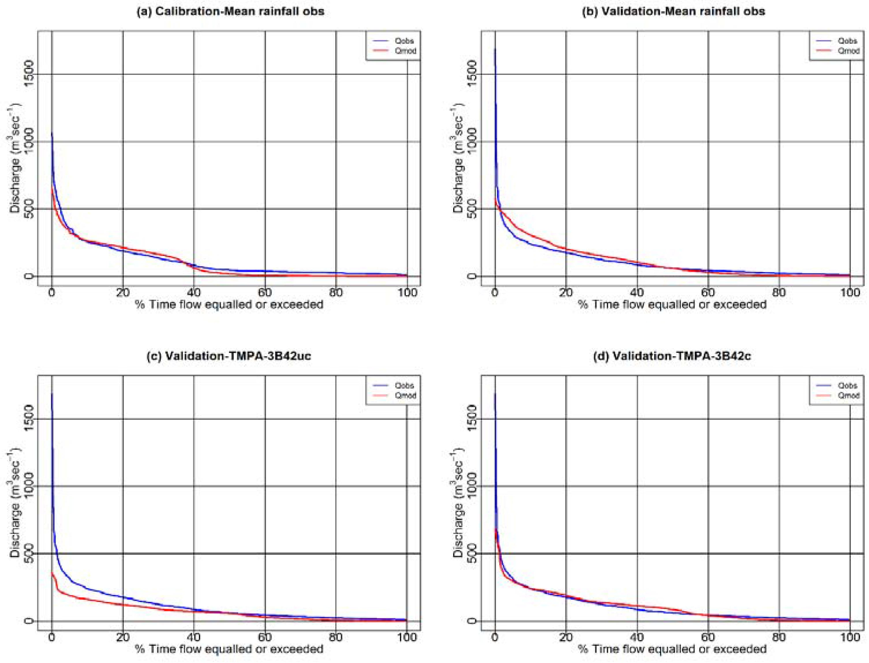
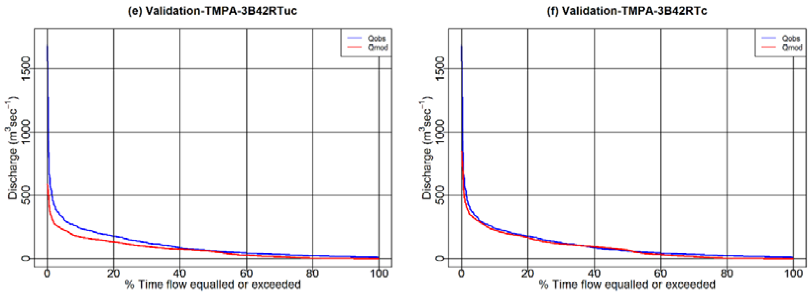
Figure 7.
Scatterplots for ten model parameters versus NSE for random parameter combinations yielding NSE > 0.5. Blue point shows the highest NSE value for the optimised parameter set.
Figure 7.
Scatterplots for ten model parameters versus NSE for random parameter combinations yielding NSE > 0.5. Blue point shows the highest NSE value for the optimised parameter set.
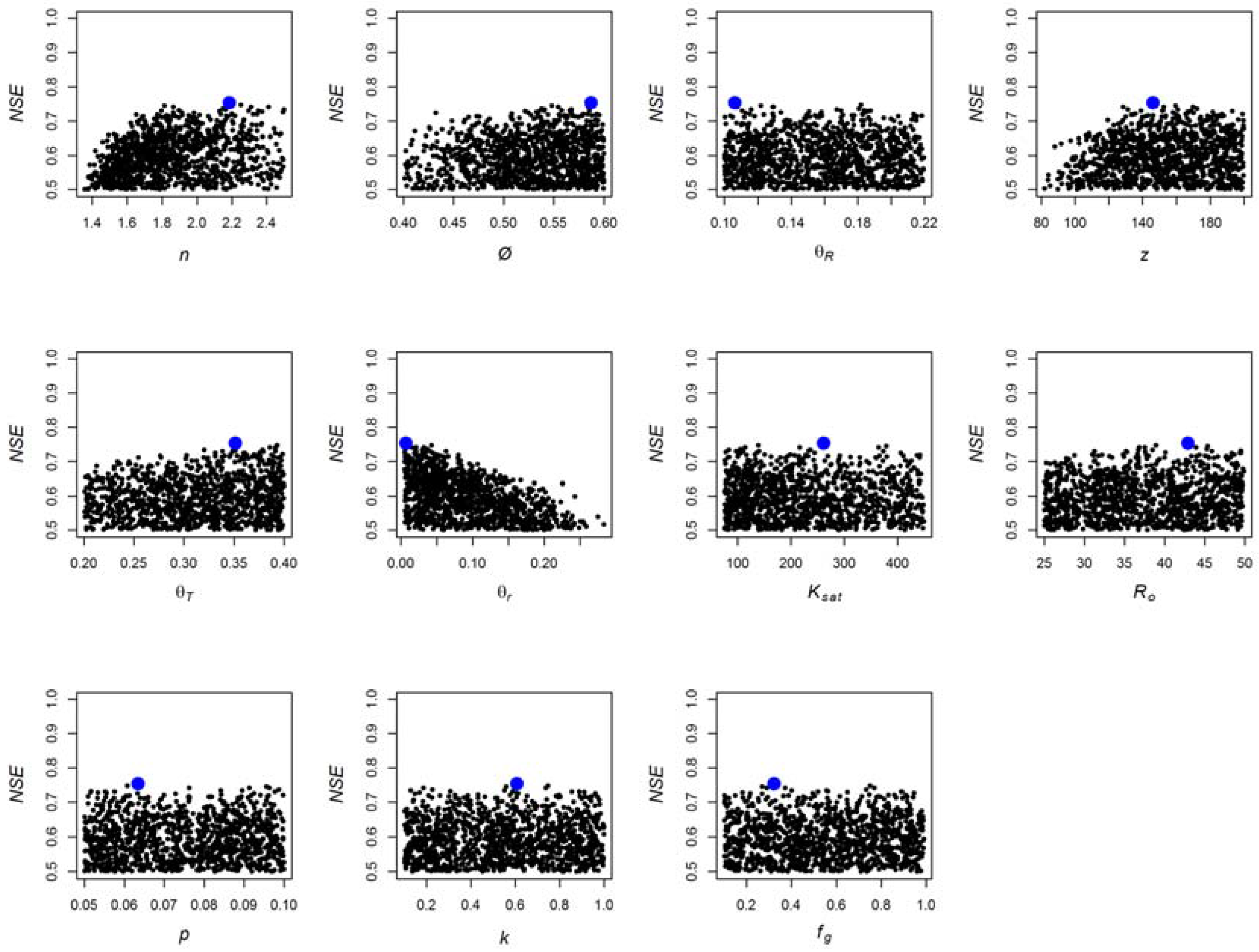
Figure 8.
Prediction uncertainty bounds for river discharge in the Lesser Zab river over the calibration period 2010–2011. The black line is the observed discharge; the red line is the median predicted flow for all combinations of parameters yielding NSE > 0.5 and the grey area shows the 95% GLUE prediction quantile. (a) All parameters sampled in the MCS; (b) Parameters to which the model was least sensitive (θT, θR, θr, p, Ro and k) fixed at their optima.


Table 1.
Optimum parameter values generated by automatic calibration for LEMSAR in the Lesser Zab catchment ( = 1).
Table 1.
Optimum parameter values generated by automatic calibration for LEMSAR in the Lesser Zab catchment ( = 1).
| Parameter | Description | Lower | Upper | Optimised Value |
|---|---|---|---|---|
| Shape parameter in van Genuchten equation (-) | 1 | 2.5 | 2.18 | |
| Saturated water content (cm3 cm−3) | 0.4 | 0.6 | 0.58 | |
| θR | Permanent wilting point (cm3 cm−3) | 0.03 | 0.22 | 0.10 |
| z | Soil depth (cm) | 50 | 200 | 146 |
| θT | Threshold water content when ET < ETₒ (cm3 cm−3) | 0.2 | 0.4 | 0.35 |
| Residual soil water content (cm3 cm−3) | 0.01 | 0.3 | 0.007 | |
| Soil saturated hydraulic conductivity (mm d−1) | 75 | 450 | 262 | |
| Rainfall threshold for overland flow (mm d−1) | 5 | 50 | 42.9 | |
| p | Fraction of excess rainfall which runs off (-) | 0.05 | 0.1 | 0.06 |
| Empirical coefficient for groundwater flow (d−1) | 0.1 | 0.99 | 0.6 | |
| Empirical partition factor for groundwater recharge (-) | 1 | 0.99 | 0.32 |
Table 2.
Summary of goodness of fit criteria for simulated discharge in the Lesser Zab catchment using different rainfall data sets to drive the model. * Significant at p ≤ 0.01.
Table 2.
Summary of goodness of fit criteria for simulated discharge in the Lesser Zab catchment using different rainfall data sets to drive the model. * Significant at p ≤ 0.01.
| Statistical Measures | Calibration | Validation | ||||
| Mean rainfall obs | Mean rainfall obs | TMPA-3B42uc | TMPA-3B42c | TMPA-3B42RTuc | TMPA-3B42RTc | |
| BIAS (%) | −12.6 | 4 | −37.6 | −2.6 | −32 | −14.2 |
| RMSE | 65 | 96 | 97 | 77 | 112 | 109 |
| NSE | 0.75 | 0.48 | 0.45 | 0.66 | 0.28 | 0.31 |
| r | 0.87 * | 0.72 * | 0.80 * | 0.81 * | 0.59 * | 0.61 * |
© 2017 by the authors. Licensee MDPI, Basel, Switzerland. This article is an open access article distributed under the terms and conditions of the Creative Commons Attribution (CC BY) license (http://creativecommons.org/licenses/by/4.0/).
Share and Cite
MDPI and ACS Style
Najmaddin, P.M.; Whelan, M.J.; Balzter, H. Application of Satellite-Based Precipitation Estimates to Rainfall-Runoff Modelling in a Data-Scarce Semi-Arid Catchment. Climate 2017, 5, 32. https://doi.org/10.3390/cli5020032
AMA Style
Najmaddin PM, Whelan MJ, Balzter H. Application of Satellite-Based Precipitation Estimates to Rainfall-Runoff Modelling in a Data-Scarce Semi-Arid Catchment. Climate. 2017; 5(2):32. https://doi.org/10.3390/cli5020032
Chicago/Turabian StyleNajmaddin, Peshawa M., Mick J. Whelan, and Heiko Balzter. 2017. "Application of Satellite-Based Precipitation Estimates to Rainfall-Runoff Modelling in a Data-Scarce Semi-Arid Catchment" Climate 5, no. 2: 32. https://doi.org/10.3390/cli5020032
Note that from the first issue of 2016, this journal uses article numbers instead of page numbers. See further details here.