Water Budget in a Tile Drained Watershed under Future Climate Change Using SWATDRAIN Model

Abstract

The SWATDRAIN model was developed by incorporating the subsurface flow model, DRAINMOD, into a watershed scale surface flow model, SWAT (Soil and Water Assessment tool), to simulate the hydrology and water quality of agricultural watersheds. The model is capable of simulating hydrology under different agricultural management and climate scenarios. As an application of the SWATDRAIN model, the impact of climate change on surface/subsurface flow was evaluated in the Canagagigue Creek watershed in southern Ontario, Canada. Using the assumption that there has been no change in land cover and land management, the model was applied to simulate annual, seasonal, and monthly changes in surface and subsurface flows at the outlet of the watershed under current and future climate conditions. The climate scenario under consideration in this study for 2015–2044 was derived from CGCM2 (Canadian Global Circulation Model 2), with A2 scenario for future climatic simulation. The SWATDRAIN model’s ability to predict the impacts of future climate change scenarios in agricultural watersheds due to monthly NSE (Nash Sutcliffe Efficiency), PBIAS (Percent Bias), and RSR (Root Mean Square Error) values of 0.74, 3.67, and 0.37, respectively, for the validation phase. The results showed that general climate change effects more spring and winter hydrology than summer hydrology. The results show that the annual flow is expected to increase in future, which will lead to an increase in the sediment loads in the stream.

1. Introduction

Changes in climate over a long time or in the short-term may exert extensive impacts on the natural hydrologic cycle and natural ecosystems, particularly in freshwater supply and in the quality of water resource systems. However, the extra precipitation would be unequally distributed around the globe. Some parts of the world may see significant reductions in precipitation, or major alterations in the timing of wet and dry seasons. Since hydrologic conditions vary from region to region, the influence of climatic change on local hydrological processes will differ within localities, even under the same climate scenarios [1]. Predictions have been made that the Canadian climate, in general, will become warmer and more variable [2]. Some recent examples of the impact of climate change on water resources include the melting of the permafrost in northern Quebec, rising sea levels in Atlantic Canada, the glacial retreat in British Columbia, and prolonged drought in the Prairies [3]. Analyzing the impact of climate change on hydrology and water quality in watersheds requires the use of hydrologic models that integrate the hydrological, chemical, and ecological processes. The Soil and Water Assessment Tool (SWAT) model [4] has been applied to several projects in the U.S. dealing with the impact of climate change on water supplies and reservoir operations, including the regional impact of climate change on the recharge of groundwater in the Ogallala aquifer [5], the impact of climate change on water yields in a high-elevation, mountainous watershed [6], the impact of climate change on the Missouri River reservoir operation and its water supply [7], and surface water irrigation and riparian management influenced by climate change [8]. A hydrological Simulation Program-FORTRAN (HSPF) model [9] was used along with two different climate change scenarios at the Credit Valley watershed in Ontario. The results of this study indicated that the warmer future climate would result in much less snowpack accumulation and greatly reduced spring freshets. The impacts of climate change on flow and water table dynamics and nitrate loads in the Ontario Greenbelt was estimated previously [10]. The effects of climate change were evaluated under the assumption that there would be no changes in land cover and land management, based on projections from the Canadian Regional Climate Model (CRCM), on the hydrology and nitrogen pollution at the outlet of a 24.3 km² agricultural watershed in Quebec using the DRAIN-WARMF model [11].

The objective of this study was to assess the impact of climate change on surface and subsurface flow in Canagagigue Creek watershed based on a Canadian climate change scenarios which has more impact on water quality. This requires a watershed scale model with the ability to accurately predict the surface and subsurface hydrology to integrate the different future climate changes scenarios. The SWATDRAIN model [10], was selected to evaluate the potential impact of the climate change on different components of water budget of Canagagigue Creek watershed, Ontario. This research will be an important contribution to the development of hydrologic models, as well as the evaluation and planning of best management practices (BMPs) for satisfying the productivity and environmental objectives under future climate conditions.

2. Materials and Methods

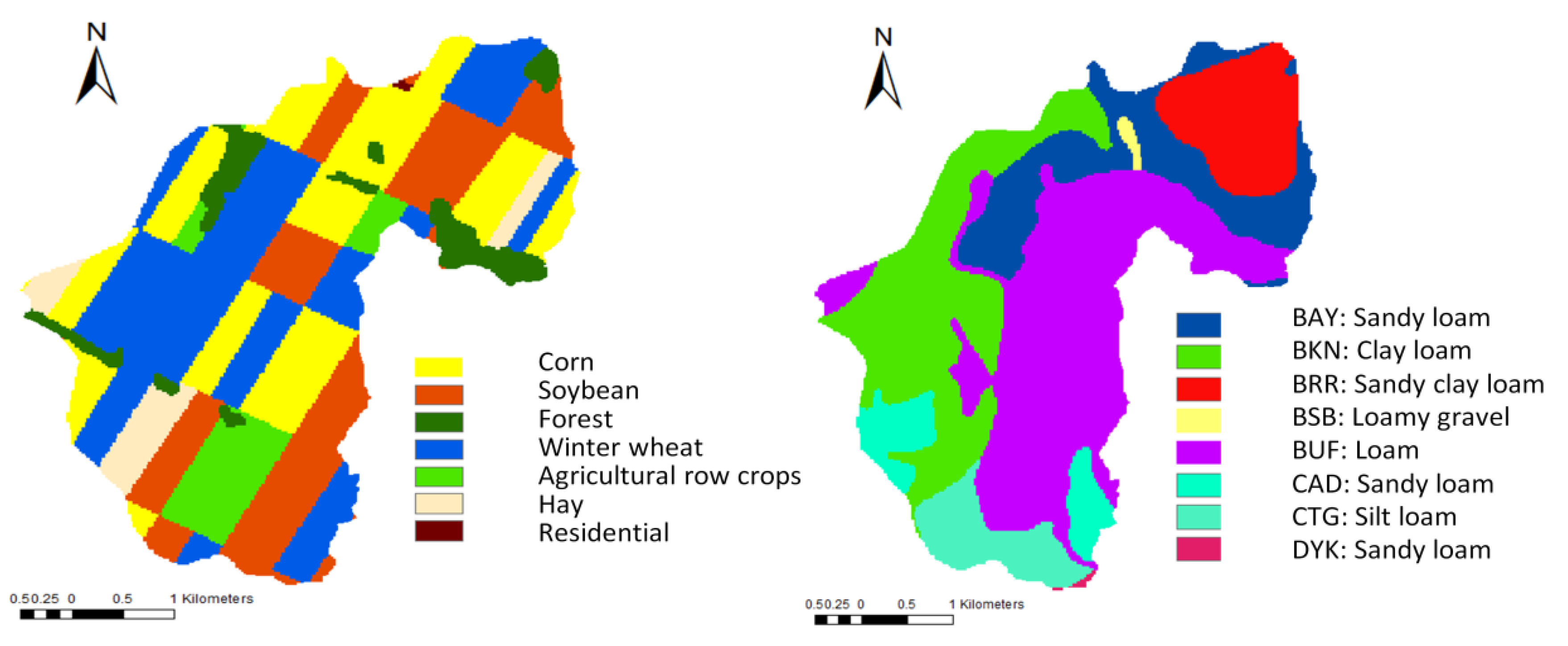
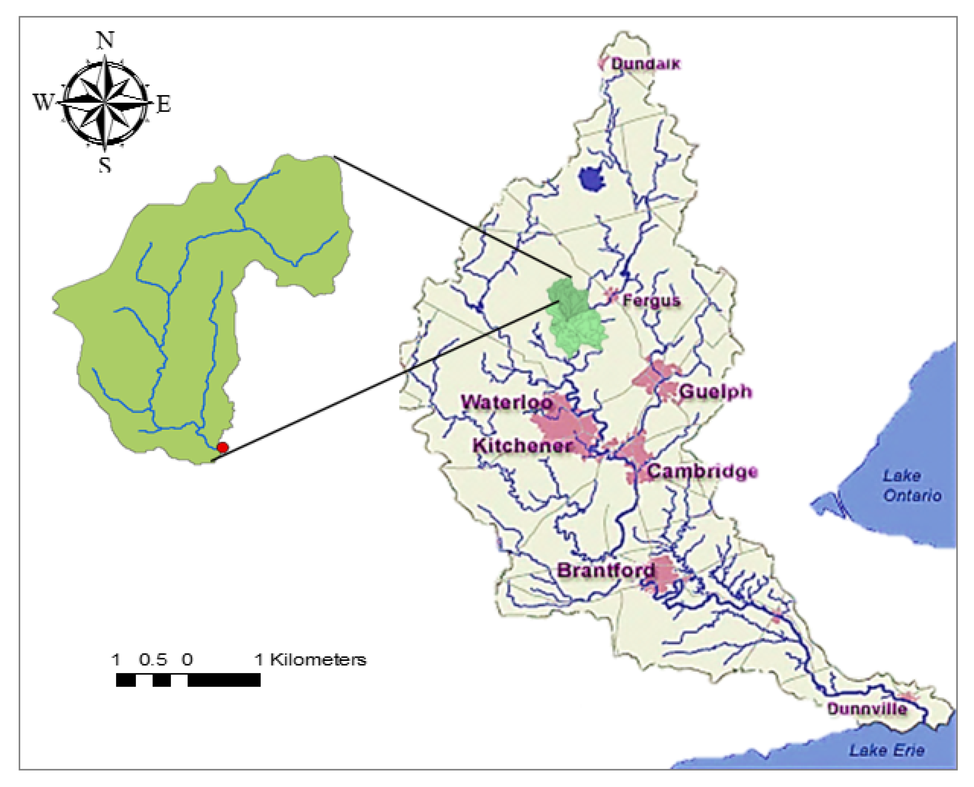
2.1. Watershed Description

The Grand River basin, located in the heart of southwestern Ontario, includes all the land drained by the Grand River and its tributaries. This large basin of almost 7000 square kilometers located in southern Ontario contributes about 10% of the drainage to Lake Erie. The watershed in this study is the Canagagigue Creek watershed near Floradle, located in the Grand River Basin in southern Ontario. The Canagagigue Creek has a total drainage area of 143 square kilometers and is a minor tributary of the Grand River. It lies between latitude 43°36’ N and 43°42’ N and longitude 80°33’ W and 80°38’ W. This study targeted the upstream portion of the Canagagigue Creek west, roughly 18 km². The watershed is approximately 19 km long, 10 km wide, and is roughly triangular. The general slope is less than 1.5%. The topography of the watershed is flat to gently undulating with a slight slope towards the outlet in the south. The average elevation is 417 m. Figure 1 shows the location of Canagagigue Creek and subwatershed used in this study.

Daily climate data were obtained from the Fergus station. A flow gage station (02GA036) is located at the stream outlet of the west branch of the watershed. The daily observations of streamflow rate were measured at this station for the period 1974–1984.

In addition to the weather data inputs, the SWAT model requires Digital Elevation Model (DEM), soils, and land use and agricultural management data, if applicable. A DEM with a 100 m × 100 m spatial resolution was obtained from the Grand River Conservation Authority. The soil and land use classification from the watershed was defined by the polygon shape files, which were provided by the Ontario Ministry of Agriculture and Food. The combination of land use and soil type resulted in 118 HRUs (Hydrologic Response Units). The soil surveys of Waterloo County [12,13] indicated that the major portion of the watershed has 200 to 600 mm of loam or silty loam of the Huron and Harriston series overlying a loam till. In the northern part of the watershed, clay loam is predominant. Loam is the main soil type in the central portion of the watershed. In the south and southeastern sections of the watershed, the soil type is comprised of moraine deposits of very fine sand and fine sandy loam, with occasional layers of other material. The topography of the watershed is flat to gently undulating with a slight slope towards the outlet in the south. Figure 2 shows the distribution of the main soil types and land use characteristics of the studied watershed. The area is composed of about 80% of agricultural land use and about 10% woodlots [14]. The rest of the watershed includes urban areas, fallow land, rivers, and lakes.

2.2. Overview of SWATDRAIN Model

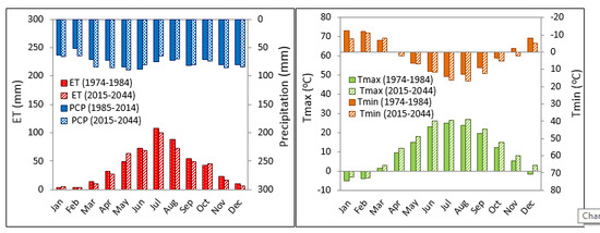
SWATDRAIN is a watershed scale model which has been developed by integrating SWAT and DRAINMOD [10]. The DRAINMOD model was incorporated into the SWAT model’s subsurface hydrology module as an alternative method for simulating tile drainage, water table depth, and soil moisture content. The newly developed SWATDRAIN model is based on the DRAINMOD subsurface hydrology simulation and the SWAT surface hydrology simulation. SWATDRAIN computes the soil water balance, on a daily basis, for each HRU in every subbasin. In the SWATDRAIN model, tile drainage values are calculated using DRAINMOD [15], which calculates drainage outflow based on Kirkham and/or Hooghoudt’s equations and the hydraulic capacity as a function of the daily water table elevation midway between the drains. In SWATDRAIN, the water table depth is calculated based on drainage volume versus the water table depth relationship, which is calculated from the soil water characteristics curve. SWATDRAIN uses either the SCS (Soil Conservation Service) curve number procedure [16], or the Green and Ampt infiltration method [17], to estimate infiltration and surface runoff. The potential evapotranspiration (PET) can be estimated using various methods available in SWATDRAIN including the Penman-Monteith method [18], the Priestly-Taylor method [19], the Hargreaves method [20], the Thornthwaite method [21], or PET can also be entered as daily or monthly PET input by the user. Detailed information on the SWATDRAIN modeling approach can be found in [10].

2.3. Climate Data

In this study, in order to develop future weather scenarios for the watershed, a Global Circulation Model (GCM) was selected for the future climatic condition simulation [22]. GCMs were developed in the 1990s and Canadian GCM (CGCM) provides several types of GCMs developed by Canada to explain the future greenhouse gases emission scenarios. There are two main families of scenarios named A and B families. The A families are more economic focused and the B scenarios are more environmental focused. They are also subdivided into scenario 1 and 2. A1 and B1 are scenarios with high globalization, while A2 and B2 illustrate a heterogeneous world emphasizing regional development. In this study, Canadian Global Circulation Model 2 (CGCM2) with A2 scenario was selected for future climate condition simulations, as the A2 scenario would have stronger adverse impacts on water quality [21]. The CGCM2 has a grid size resolution of 417 km × 342 km, which is very coarse for watershed scale modeling, and hence downscaling is needed. Therefore, we selected the SDSM (Statistical Downscaling Model) downscaling tool as it is robust, well tested [23,24,25], and capable of performing various analyses and producing variety of outputs.

3. Results and Discussion

3.1. Model Evaluation

The SWATDRAIN model was recently calibrated and validated for streamflow and sediment loads at Canagagigue Creek watershed [26]. The Green and Ampt infiltration method [17] was used to estimate infiltration and surface runoff. The potential evapotranspiration (PET) was estimated using the Thornthwaite method [21]. Detailed information on the SWATDRAIN modeling approach can be found in previous studies [10,27].

The results showed that the observed and simulated streamflows were in good agreement. During the calibration period, the model closely simulated streamflow values. The calibration and validation model performance results for the daily and monthly streamflow and sediment loads are presented in

Table 1. SWATDRAIN statistics for the Canagagigue Creek watershed on monthly and daily time steps streamflow and sediment loads (Adopted from 14). RSR, Root Mean Square Error; NSE, Nash Sutcliffe Efficiency; PBIAS, Percent Bias.

Index	Monthly		Daily		Monthly		Daily
	Calibration	Validation	Calibration	Validation	Calibration	Validation	Calibration	Validation
R2	0.92	0.82	0.85	0.75	0.88	0.89	0.82	0.73
RSR	0.27	0.37	0.36	0.47	0.41	0.44	0.48	0.49
PBIAS	−6.07	3.67	−6.07	3.67	−1.71	25.88	−1.71	25.88
NSE	0.88	0.74	0.78	0.60	0.83	0.80	0.74	0.71

.

During the calibration period, the monthly and daily NSE (Nash Sutcliffe Efficiency) values were 0.88 and 0.78 for streamflow and 0.83 and 0.74 for sediment, respectively. While the PBIAS (Percent Bias) values at the monthly and daily time steps were −6.07 and −1.71 for streamflow and sediment loads, respectively (Table 1). Therefore, the SWATDRAIN model was well calibrated, as shown by the statistics in Table 1. The monthly NSE, PBIAS, and RSR (Root Mean Square Error) values for the streamflow during the validation phase were calculated to be 74.00, 3.67, and 0.37, respectively (Table 1). For the sediment loads, the monthly NSE, PBIAS, and RSR values were calculated to be 0.80, 25.88, and 0.44, respectively, during the validation phase (Table 1). Therefore, in this study, the streamflow simulation performance was good according to the hydrologic model evaluation guidelines [28].

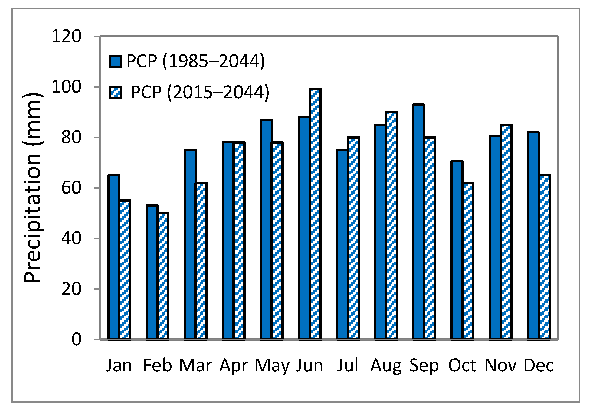
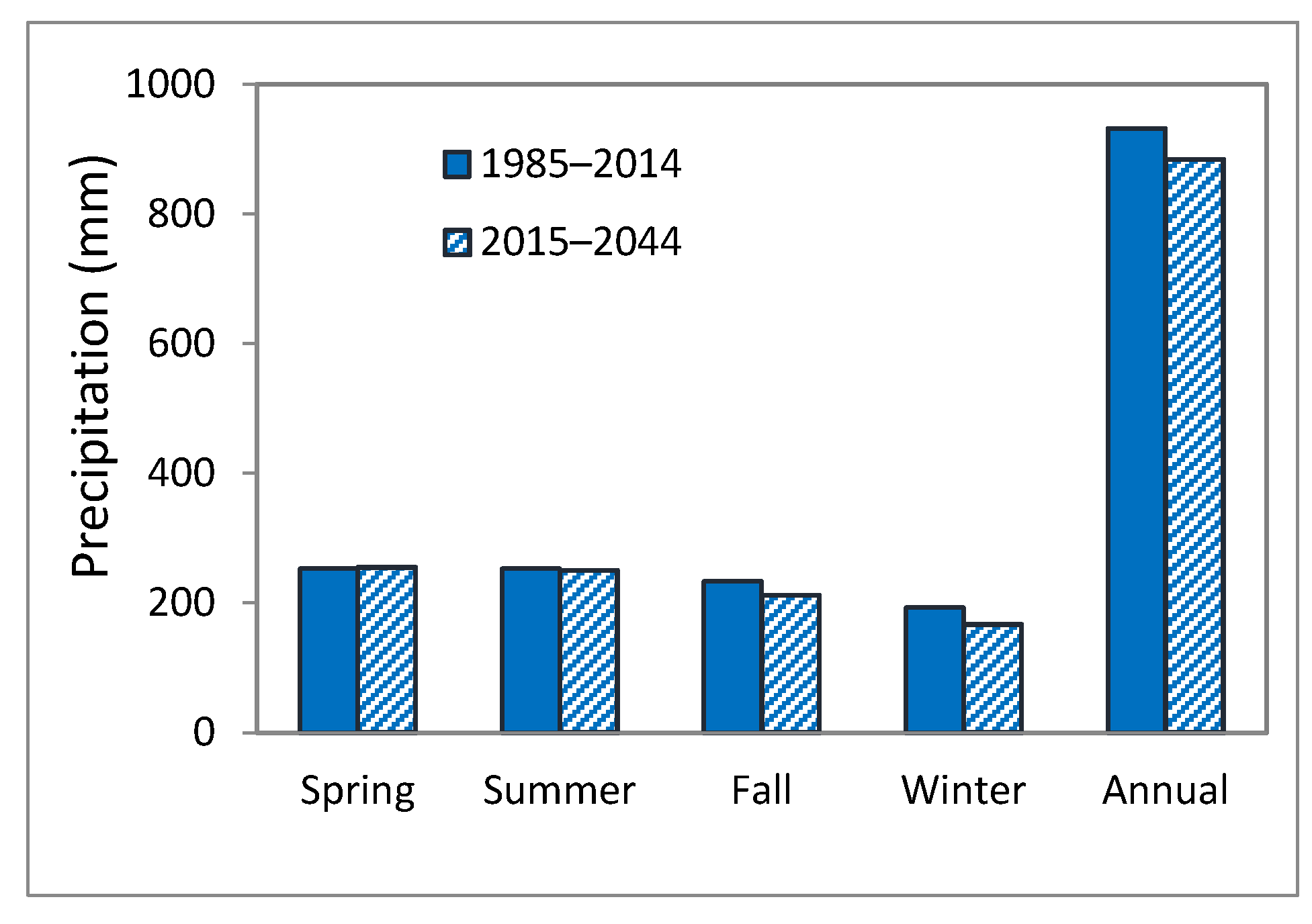
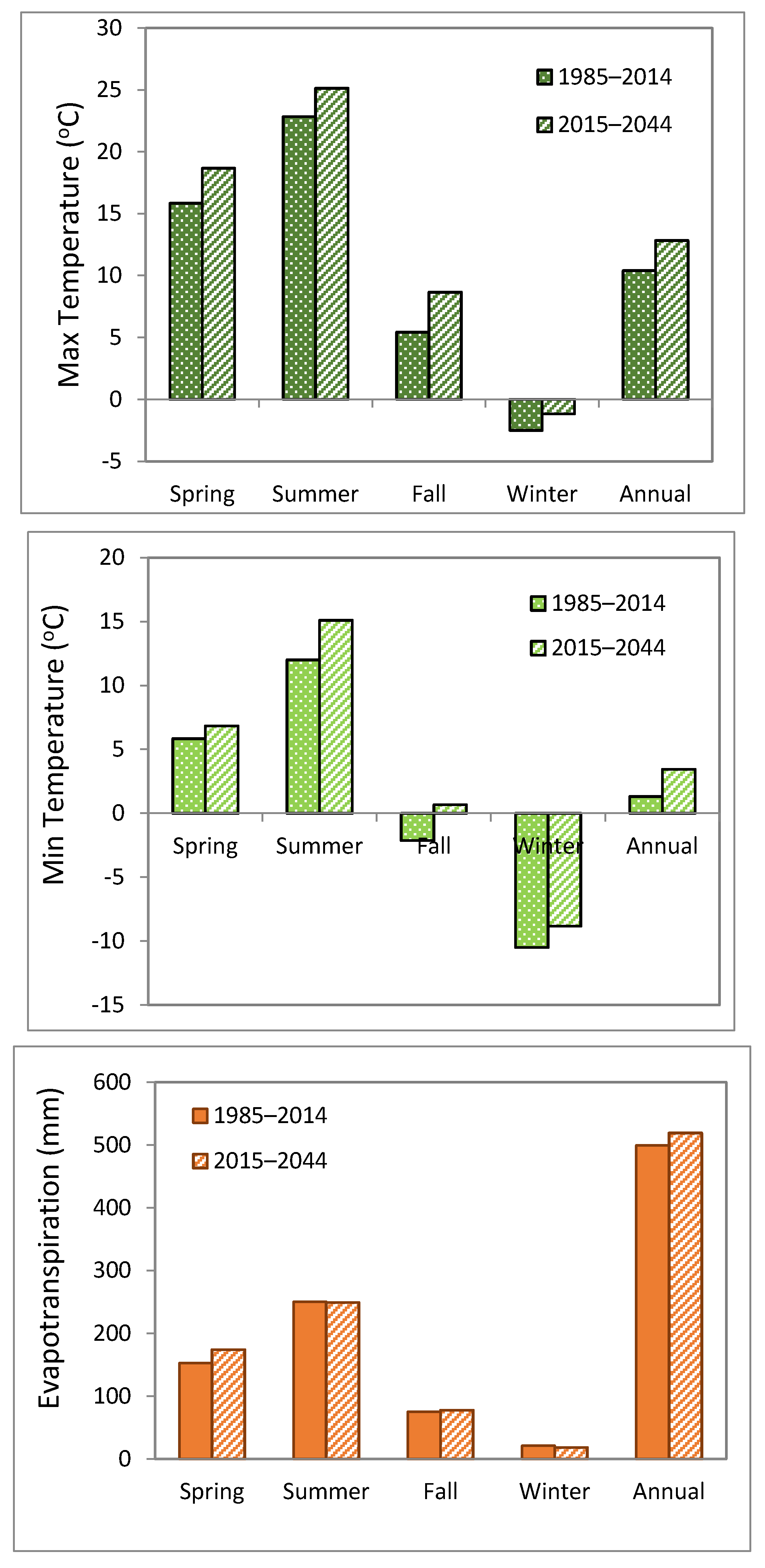
3.2. Climate Change Scenario

3.2.1. SDSM Calibration, Validation, and Evaluation

The SDSM downscaling tool is calibrated using the historical observed weather variables from 1961 to 1990 including daily maximum temperature (T_max in °C), minimum temperature (T_min in °C), and daily mean precipitation (P_mean in mm) from Fergus weather station in Ontario to simulate downscaled variables. Validation was performed from 1991 to 2001 without changing any linear regression parameters within the SDSM tool. During calibration and validation, several statistic evaluation coefficients, for example, NSE (Nash Sutcliffe Efficiency), RMSE (Root Mean Square Error), and Regression Coefficient (R²) were used to evaluate the performance of SDSM (NSE: 0.994, 0.992, and 0.71 for T_max, T_min, and P_mean, respectively). Upon satisfactory calibration and validation, the same parameters were used for the future CGCM2 (A2 scenario) from 2015 to 2044 to derive the future daily climate weather variables.

3.2.2. Time Series Analysis

The non-parametric Kolmogorov-Smirnov two-sample test (KS test) was used for distribution analysis of the monthly averaged T_max, T_min, and P_mean. The p-values of each month at 95% confidence level for the observed and corresponding downscaled predictands were computed by MYSTAT12 (SYSTAT Software version 12, 2007).

Table 2. p-Values of Kolmogorov-Smirnov two-sample test (KS Test) for observations and downscaled predictands (Historical).

Predictands	Jan.	Feb.	Mar.	Apr.	May	Jun.	Jul.	Aug.	Sep.	Oct.	Nov.	Dec.
Tmax	0.546	0.546	0.546	0.172	0.797	0.546	0.797	0.323	0.172	0.969	0.969	0.546
Tmin	0.546	0.172	0.172	0.323	0.172	0.130	0.546	0.323	0.35	0.082	0.797	0.172
Pmean	0.082	0.035	0.172	0.130	0.172	0.035	0.035	0.088	0.172	0.797	0.323	0.082

presents the p-values of each month for each pair of observed weather and downscaled predictands.

The p-values less than 0.05 indicate significant difference in the distribution of observed and downscaled predictands. It is apparent from Table 2 that T_max gives the best distribution test results, which is better than T_min, and in turn, downscaling of T_min is better than the P_mean.

One important issue is to identify the temporal changes in hydrological regimes of watersheds because of the potential impact of climate change on river flow regimes [29]. The purpose is to understand any existing climate change trend and whether the predicted future variables follow similar patterns to the observed trends.

Table 3. Summary of downscaled weather predictands trend analysis (2015–2044).

Predictands	Items	Jan.	Feb.	Mar.	Apr.	May	Jun.	Jul.	Aug.	Sep.	Oct.	Nov.	Dec.
Tmax	Slope	0.070	0.089	0.046	0.109	0.042	0.006	0.019	−0.008	0.030	0.023	0.028	0.036
	p-value	0.055	0.089	0.259	0.142	0.349	0.816	0.374	0.730	0.141	0.388	0.332	0.087
Tmin	Slope	0.135	0.128	0.051	0.063	0.026	0.005	0.026	0.005	0.026	0.009	0.015	0.041
	p-value	0.022	0.062	0.372	0.213	0.352	0.839	0.237	0.783	0.192	0.714	0.500	0.013
Pmean	Slope	0.000	−0.002	−0.005	0.001	0.001	0.012	0.007	0.016	0.002	0.004	0.000	0.004
	p-value	0.960	0.624	0.535	0.938	0.256	0.524	0.515	0.259	0.835	0.788	0.981	0.491

summarize the slopes of the trend lines and the associated p-values of monthly predictands.

For the future period, the monthly averaged T_max might have a statistically significant change trend, except for the months of January, February, and March. The future monthly T_min in each month might be increasing for the future period, except January and February. The change of P_mean in the future for each month might be negligible. The average monthly total precipitation for the historical period and future periods are presented in Figure 3.

The results indicate that in the months of June, July, and August the future monthly precipitation was greater than those in the historical period, while, in other months, the future monthly total precipitations were less than those historically. This is also confirmed in Figure 4, which shows in summer the future precipitation was greater than the historical, while in other seasons the future precipitations were less. Due to future temperature changes, warmer winters and hotter summers are expected, which will lead to more evaporated water loss (Figure 3 and Figure 4).

3.3. Future Simulations

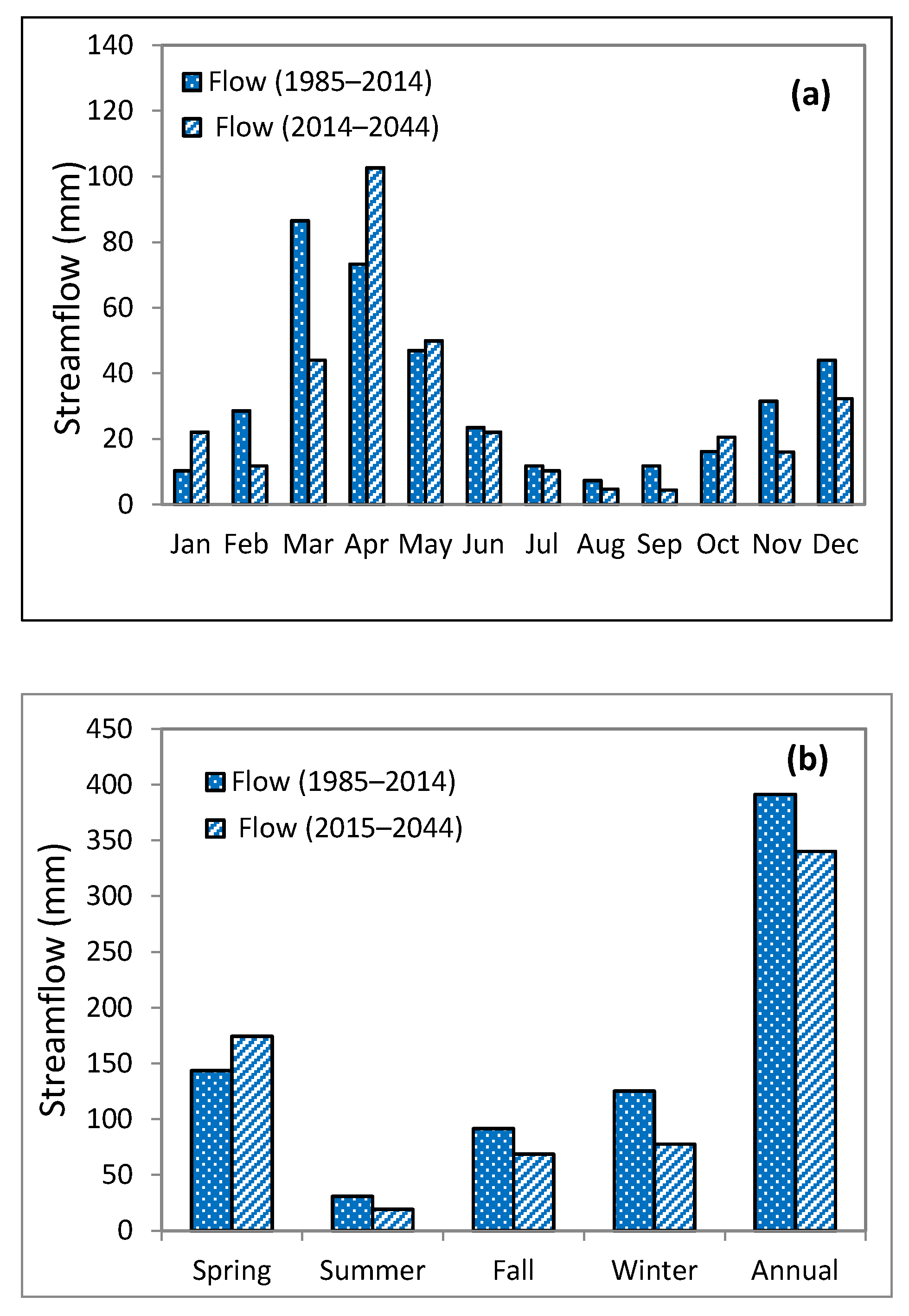
3.3.1. Streamflow

The climate change impacts of subsurface drainage on hydrology was evaluated by running the SWATDRAIN model for the climate data from 1985–2014 (historical) and 2014–2044. Once the SWATDRAIN model was calibrated and validated, the CGCM2 daily weather predictands downscaled by SDSM (i.e., daily precipitation, maximum temperature, minimum temperature) were imported as the new weather variables for the future period of 2014–2044. The model was run from 2010 to 2044 by giving five years to warm up the initial parameters. The average monthly and seasonal streamflow during both the historical and the future period were compared to see the monthly change patterns, which are presented in Figure 5. Figure 5 shows that the streamflow in March decreased significantly in the future period, while in January and May it was slightly increased. Figure 5 also shows that the streamflow decreased in each season. From Figure 5 it was noted that the highest monthly total streamflow for the historical period was March, while for the future period the highest monthly flow occurred in April. This might be explained by the fact that the precipitation projected gives less precipitation in winter than the historical period (Figure 3, Figure 4 and Figure 5). Therefore, the possible later snowfall or later river freezing plus increased temperature may cause faster snowmelt during the winter not only for Match, but also for other months such as January and February.

This resulted in a smaller flow rate in March. In addition, the precipitation plays a more important role on streamflow generation in winter and spring. Thus, the highest flow peaks may shift to April due to high precipitation and low evapotranspiration. It seems like in the future, due to climate change, much more evapotranspiration may be expected, and thus the total water yield may decrease significantly. This could represent a severe water resource loss in the future which could be caused by less precipitation in winter, spring, and fall, and higher evapotranspiration.

The increase in streamflow during winter and early spring periods is mainly the result of higher minimum daily temperatures as well as changes in precipitation regimes from snowfall to rainfall during winter and early spring periods.

Table 4. Water Balance Components for Historical (1985–2014) and Future (2015–2044) Periods.

Component	Historical		Future
	Value (mm)	%	Value (mm)	(%)
Precipitation	975.8	100	937.0	100
ET	475.3	48.70	525.5	56.08
Stream Flow	392.4	40.21	339.5	36.23
Base Flow	143.4	14.69	152.8	16.30
Snowmelt	108.1	11.08	72	7.68

shows the changes in snowmelt between the historical and future periods. Overall the average future snowmelt is reduced due to reduction in total precipitation. In average, the snowmelt accounts for 11.08 percent of the precipitation in historical period and 7.68 percent in the future period. This water is generally added to runoff and infiltration in late winter and early spring.

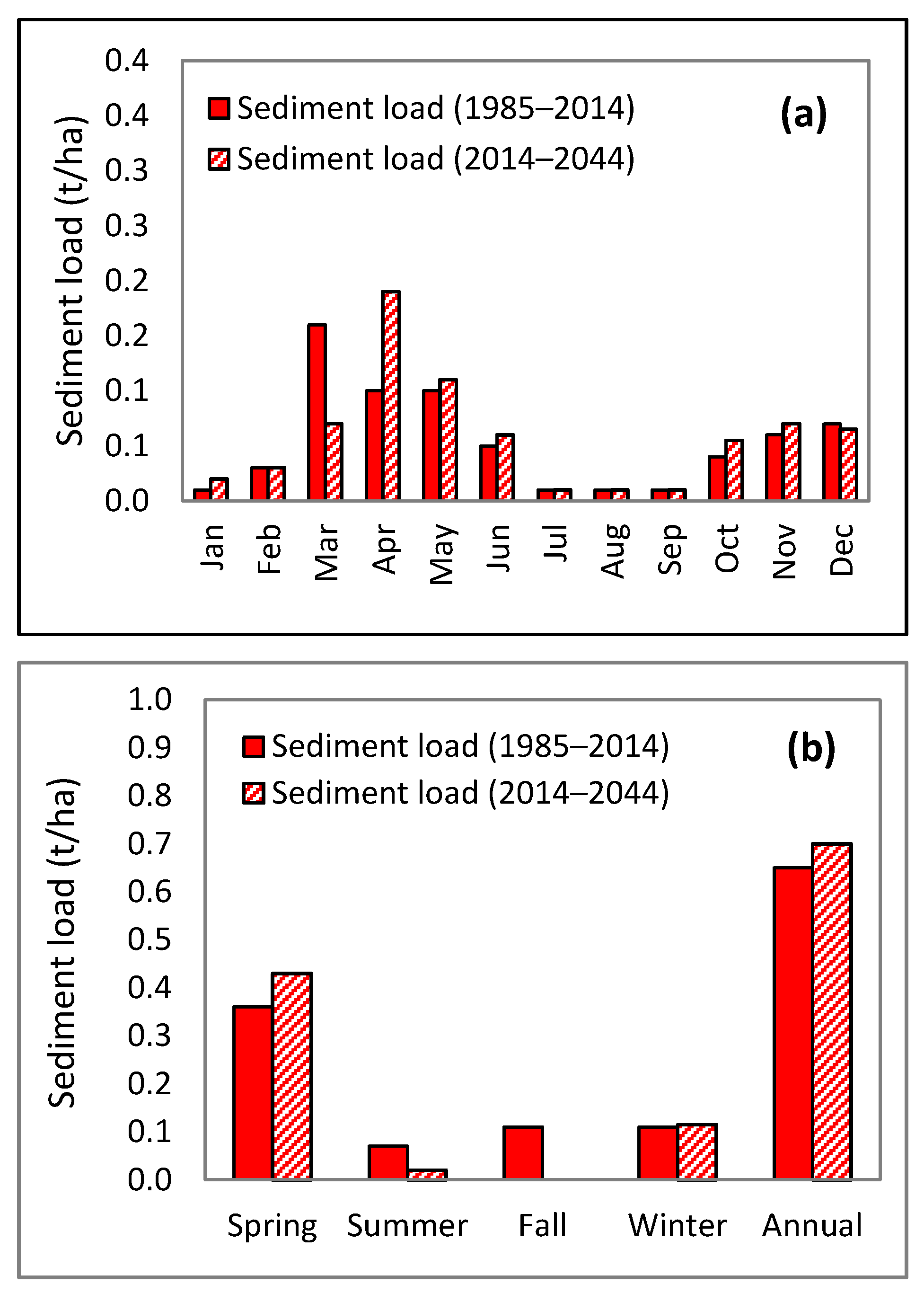
3.3.2. Sediment Loads

The impact of changed hydrology on sediment loads in the Canagagigue Creek watershed was assessed using the SWATDRAIN model. The average monthly and seasonal sediment loads during both the historical period and the future period were compared in order to determine the monthly change patterns (Figure 6). The peaks of the monthly total sediment loads occurred in the same months of peak flows. It was noted that the magnitudes of peaks in the future period were less than those of the historical period.

Figure 6 indicates that in the future April may be the only month with high sediment load. A decrease of sediment in March was mainly caused by the significant decrease in streamflow in this month. Therefore, spring was the only season with high sediment yields, indicating relatively high sediment capacity in spring.

4. Conclusions

This study presents the impact of climate change, based on projections from the CGCM2, A2 scenario on the hydrology of an agricultural watershed in the cold climate of Ontario.

The SWATDRAIN model [10] was evaluated for the water budget at the Canagagigue Creek watershed of Ontario, Canada. The results from a previous study [10,27] demonstrate that the SWATDRAIN model adequately simulated the hydrology of the watersheds and performed satisfactory results. The validated SWATDRAIN model at the same study area was applied for the historical (1960–1990) and future (2015–2045) climate data, and the potential impact of climate change on monthly, seasonal, and annual streamflow was evaluated.

The results indicated that due to climate change, the temperature will be increased significantly. In terms of the future weather change, warmer winters and hotter summers might be expected. The increase in min/max temperatures in winter would lead to more rainfall-dominated regime and less snowfall. This would result in an increase in length of the growing season. Therefore, the climate change projected for this region seems likely to alter both magnitude and seasonality of flow. The results show that the annual flow is expected to decrease due to climate change in the future, which will lead to a decrease in the sediment loads in the stream. It is important to note this may not mean that in the future the sediment load as a pollution would be mitigated. It also could result in severe low flows in streams with decreased channel carrying capacity. It can be concluded that the sediment deposition may be a common phenomenon in the future.

References

1. Zhang, X.; Srinivasan, R.; Hao, E. Predicting hydrologic response to climate change in the Luohe River basin using the SWAT model. Trans. ASABE 2007, 50, 901–910. [Google Scholar] [CrossRef]
2. Hengeveld, H.G. Projections for Canada’s climate future: A discussion of recent simulations with the canadian global climate model. In Climate Change Digest Special Edition CCD 00–01; Meteorological Service of Canada Environment Canada: Downsview, ON, Canada, 2000. [Google Scholar]
3. Mehdi, B.; Connolly-Boutin, L.; Madramootoo, C.A. Coping with the Impacts of Climate Change on Water Resources: A Canadian Experience. World Res. Rev. 2006, 18, 62. [Google Scholar]
4. Arnold, J.G.; Fohrer, N. SWAT2000: Current capabilities and research opportunities in applied watershed modeling. Hydrol. Process. 2005, 19, 563–572. [Google Scholar] [CrossRef]
5. Rosenberg, N.J.; Epstein, D.J.; Wang, D.; Vail, L.; Srinivasan, R.; Arnold, J.G. Possible Impacts of Global Warming on the Hydrology of the Ogallala Aquifer Region. Clim. Chang. 1999, 42, 677–692. [Google Scholar] [CrossRef]
6. Stonefelt, M.D.; Fontaine, A.T.; Hotchkiss, R.H. Impacts of Climate Change on Water Yield in the Upper Wind River Basin. Am. Water Res. Assoc. 2000, 36, 321–336. [Google Scholar] [CrossRef]
7. Hotchkiss, R.H.; Jorgensen, S.F.; Stone, M.C.; Fontaine, T.A. Regulated River Modeling for Climate Change Impact Assessment: The Missouri River. Am. Water Res. Assoc. 2000, 36, 375–386. [Google Scholar] [CrossRef]
8. Wollmuth, C.J.; Eheart, J.W. Surface Water Withdrawal Allocation and Trading Systems for Traditionally Riparlan Areas. Am. Water Res. Assoc. 2000, 36, 293–303. [Google Scholar] [CrossRef]
9. Bicknell, B.R.; Imhoff, J.C.; Kittle, J.L.; Donigian, A.S.; Johanson, R.C. Hydrologic Simulation Program: Fortran; User Manual for Release 11; United States Environmental Protection Agency: Washington, DC, USA, 1996.
10. Golmohammadi, G.; Prasher, S.; Madani, A.; Rudra, R.; Youssef, M.A. SWATDRAIN, a new model to simulate the hydrology of agricultural lands, model development and evaluation. J. Biosyst. Eng. 2016, 141, 31–47. [Google Scholar] [CrossRef]
11. Dayyani, S.; Prasher, S.O.; Madani, A.; Madramootoo, C.A. Impact of climate change on the hydrology and nitrogen pollution in a tile-drained agricultural watershed in eastern Canada. Trans. ASABE 2012, 55, 398–401. [Google Scholar] [CrossRef]
12. Presant, E.W.; Wicklund, R.E. Soil Survey of Waterloo County; Report No. 44 of the Ontario Soil Survey Canada; University of Guelph: Guelph, ON, Canada, 1971. [Google Scholar]
13. Hoffman, D.W.; Matthews, B.C.; Wicklund, R.E. Soil survey of Wellington County Ontario; Report No.35; Ontario Soil Survey, Department of Agriculture and Ontario Department of Agriculture: Guelph, ON, Canada, 1963.
14. Carey, J.H.; Fox, M.E.; Brownlee, B.G.; Metcalfe, J.L.; Mason, P.D.; Yerex, W.H. The Fate and Effects of Contaminant in Canagagigue Creek 1. Stream Ecology and Identification of Major Contaminants; Environment Canada: Burlington, ON, Canada, 1983.
15. Skaggs, R.W. Methods for Design and Evalua-tion of Drainage-Water Management Systems for Soils with High Water Tables; South National Technical Center: Missouri, MS, USA, 1980. [Google Scholar]
16. Soil Conservation Service (SCS). National Engineering Handbook; USDA Soil Conservation Service: Washington, DC, USA, 1972.
17. Green, W.H.; Ampt, G.A. Studies on soil physics: Part I. The flow of air and water through soils. J. Agric. Sci. 1991, 4, 1–24. [Google Scholar]
18. Monteith, J.L. Evaporation and environment. Symposium. Soc. Exp. Biol. 1965, 19, 205–234. [Google Scholar]
19. Hargreaves, G.H.; Samani, Z.A. Reference crop evapotranspiration from temperature. Appl. Eng. Agric. 1985, 1, 96–99. [Google Scholar] [CrossRef]
20. Priestley, C.H.B.; Taylor, R.J. On the assessment of surface heat flux and evaporation using large-scale parameters. Mon. Weather Rev. 1972, 100, 81–92. [Google Scholar] [CrossRef]
21. Thornthwaite, C.W. An Approach toward a Rational Classification of Climate. Geogr. Rev. 1948, 38, 55–94. [Google Scholar] [CrossRef]
22. Rong, H. Water Quality Evaluation under Climate Change Impacts for Canagagigue Creek Watershed in Southern Ontario. Master’s Thesis, Department of Civil Engineering, Guelph University, Guelph, ON, Canada, 2009. [Google Scholar]
23. Khan, M.S.; Coulibaly, P.; Dibike, Y. Uncertainty analysis of statistical downscaling methods using canadian global climate model predictors. Hydrol. Process. 2006, 20, 3085–3104. [Google Scholar] [CrossRef]
24. Harpham, C.; Wilby, R.L. Multi-site downscaling of heavy daily precipitation occurrence and amounts. J. Hydrol. 2005, 312, 235–255. [Google Scholar] [CrossRef]
25. Dibike, Y.B.; Coulibaly, P. Validation of hydrological models for climate scenario simulation: The case of saguenay watershed in quebec. Hydrol. Process. 2007, 21, 3123–3135. [Google Scholar] [CrossRef]
26. Golmohammadi, G.; Prasher, R.P.; Rudra, A.; Madani, M.; Youssef, M.; Goel, P. Impact of Tile Drainage on Water Budget and Spatial Distribution of Sediment Generating Areas in an Agricultural Watershed. J. Agric. Manag. 2017, 184, 124–134. [Google Scholar] [CrossRef]
27. Golmohammadi, G.; Rudra, R.P.; Prasher, S.O.; Madani, A.; Goel, P.K.; Mohammadi, K. Effect of Controlled Drainage on Watershed Hydrology. Arab. J. Geosci. 2016, 9, 3–7. [Google Scholar] [CrossRef]
28. Moriasi, D.N.; Arnold, J.G.; Van Liew, M.W.; Bingner, R.L.; Harmel, R.D.; Veith, T.L. Model evaluation guidelines for systematic quantification of accuaracy in watershed simulations. Trans. ASABE. 2007, 50, 885–900. [Google Scholar] [CrossRef]
29. He, H.; Zhou, J.; Zhang, W. Modeling the impacts of environmental changes on hydrological regimes in the Hei river watershed, China. Glob. Planet. Chang. 2008, 61, 175–193. [Google Scholar] [CrossRef]
Figure 1. Location of study area.
Climate 05 00039 g001
Figure 2. Land use and soil type maps.
Climate 05 00039 g002
Figure 3. Historical and future predicted monthly average precipitation, temperature, and evapotranspiration. ET, Evapotranspiration; PCP, Precipitation
Climate 05 00039 g003aClimate 05 00039 g003b
Figure 4. Historical and future seasonal precipitation, evapotranspiration and temperature.
Climate 05 00039 g004aClimate 05 00039 g004b
Figure 5. Historical and future simulated monthly (a) and seasonal (b) streamflow.
Climate 05 00039 g005
Figure 6. Historical and future simulated monthly (a) and seasonal (b) sediment loads.
Climate 05 00039 g006