
Evaluating the Effect of Physics Schemes in WRF Simulations of Summer Rainfall in North West Iran

1
Atmospheric Science & Meteorological Research Center (ASMRC), Tehran P.O. Box 14977-16385, Iran
2
Water Engineering Department, University of Guilan, Rasht P.O. Box 41889-58643, Iran
*
Author to whom correspondence should be addressed.
Climate 2017, 5(3), 48; https://doi.org/10.3390/cli5030048
Submission received: 3 May 2017
/
Revised: 27 June 2017
/
Accepted: 2 July 2017
/
Published: 6 July 2017
Abstract
:The numerical weather forecast model Weather Research and Forecasting (WRF) has a range of applications because it offers multiple physical options, enabling the users to optimizing WRF for specific scales, geographical locations and applications. Summer rainfall cannot be predicted well in North West of Iran (NWI). Most of them are convective. Sometimes rainfall is heavy, so that it causes flash flood. In this research, some configurations of WRF were tested with four summer rainfall events in NWI to find the best configuration. Five cumulus, four planetary boundary layers (PBL) and two microphysical schemes were combined. Twenty-six different configurations (models) were implemented at two resolutions of 5 and 15 km for duration of 48 h. Four events, with over 20 mm convective daily rainfall total, were selected at NWI during summer season between 2010 and 2015. These events were tested by developing 26 unique models. Results were verified using several methods. The aim was to find the best results during the first 24 h. Although no single configuration can be introduced for all times, thresholds, and atmospheric system to provide reliable and accurate forecast, the best configuration for WRF can be identified. Kain-Fritsch (new Eta), Betts-Miller-Janjic, Modified Kain-Fritsch, Multi-scale Kain-Fritsch and newer Tiedtke cumulus schemes and Mellor-Yamada-Janjic, Shin-Hong ‘scale-aware’, Medium Range Forecast (MRF) and Yonsei University (YSU) Planetary Boundary Layer schemes and Kessler, WRF Single Moment 3 class simple ice (WSM3) microphysics schemes were selected. The result show that Cumulus schemes are the most sensitive and Microphysics schemes are the less sensitive. The comparison of 15 km and 5 km resolution simulations do not show obvious advantages in downscaling the results. Configuration with newer Tiedtke cumulus, Mellor-Yamada-Janjic PBL, WSM3 and Kessler microphysics schemes give the best results for the 5 and 15 km resolutions. The output image of models and statistical methods verification indexes show that WRF could not accurately simulate convective rainfall in the NWI in summer.
1. Introduction
In the Northwestern area of Iran about half of the annual precipitation occurs between months of March and May. Less than 4% of the annual precipitation occurs in summer [1], typically with heavy convective rainfall. Topography and other factors provide favorable conditions for the occurrence of flood in this area in summer. There is a rising cost and social impact associated with extreme weather, not to mention the loss of human life [2]. These events have major effects on the society, economy and the environment [3], and have a direct impact on people, countries and vulnerable regions [4]. Records show that these events are increasing [5]. There are several methods to predict rainfall-runoff. Rainfall-runoff modeling was improved in many researches [6,7,8,9,10].
An important thing to predict flash flood is heavy rainfall forecasting. If we can predict rainfall, it will be very useful to determine flash flood. An attempt to seek a relatively optimal data-driven model for rainfall forecasting from three aspects: model inputs, modeling methods, and data-preprocessing techniques. A proposed model, modular artificial neural network (MANN), is compared with three benchmark models, viz. artificial neural network (ANN), K-nearest-neighbors (K-NN), and linear regression (LR). The proposed optimal rainfall forecasting model can be derived from MANN coupled with SSA [11]. In this study, Numerical weather prediction (NWP) was used to improve rainfall simulation.
According to statistical data from 87 meteorological stations, 132 cases have been recorded with daily rainfall total over 20 mm in this region during the summer since 1954 to 2015, and 41 cases have recorded in the last 5 years. These few events during the summer since 1954 to 2015 because there were a few stations before 2000 and the most of weather stations were stablished after that. For example 41 events were recorded in 5 years between 2010 and 2015. All 87 weather stations had data during 2010 to 2015 and their data is reliable [12], then historical records of 2010 to 2015 are taken.
Most of these events have not been predicted. Then we need to improve our rainfall simulation. The WRF system is a mesoscale numerical weather prediction system used for operational forecasting, which allows users to make adjustments for a specific scale and geographical location [13]. Four different WRF microphysics schemes have been tested [14] over southeast India (Thompson, Lin, WRF Single-Moment 6 class (WSM6) and Morrison). While the Thompson scheme simulated surface rainfall distribution closer to observations, the other three schemes overestimated observed rainfall. Furthermore [15], Austral summer rainfall over the period 1991/1992 to 2010/2011 was dynamically downscaled by the WRF model at 9 km resolution for South Africa, and utilized three different convective parameterization schemes, namely the (1) Kain-Fritsch (KF), (2) Betts-Miller-Janjic (BMJ) and (3) Grell-Devenyi-ensemble (GDE) schemes. All three schemes have generated positive rainfall biases over South Africa, with the KF scheme producing the largest biases and mean absolute errors. Only the BMJ scheme could reproduce the intensity of rainfall anomalies, and also exhibited the highest correlation with the observed internal summer rainfall variability. In another study [16], simulations of a 15 km grid resolution were compared using five different cumulus parameterization schemes for three flooding events in Alberta, Canada. The Kain-Fritsch and explicit cumulus parameterization schemes were found to be the most accurate when simulating precipitation across three summer events.
The accuracy of South East of United State (SE US) summer rainfall simulations at 15 km resolution were evaluated [17] using (WRF) model and were compared with those at the 3 km resolution. Results indicated that the simulations at the 3 km resolution do not show significant advantages over those at the 15 km resolution using the Zhang-McFarlane cumulus scheme. In this study it was suggested that to obtain an acceptable simulation, selection of a suitable cumulus scheme that realistically represents the convective rainfall triggering mechanism is more important than just increasing the model resolution. Another study [18] has evaluated the WRF model for regional climate applications over Thailand, focusing on simulated precipitation using various convective parameterization schemes possible in WRF. Experiments were carried out for the year 2005 using four convective cumulus parameterization schemes, namely, Betts-Miller-Janjic (BMJ), Grell-Devenyi (GD), improved Grell-Denenyi (G3D) and Kain-Fritsch (KF) with and without nudging applied to the outermost nest. The results showed that the experiments with nudging generally performed better than un-nudged experiments and that the BMJ cumulus scheme with nudging provided the smallest bias relative to the observations. Another study [19] that examined the sensitivity of the WRF model performance using three different PBL schemes Mellor-Yamada-Janjic (MYJ), Yonsei University (YSU), and the asymmetric convective model, version 2 (ACM2) WRF simulations with different schemes over Texas in July–September 2005 showed that the simulations with the YSU and ACM2 schemes gave much less bias compared to the MYJ scheme. An examination combined different physical scheme for simulation series of rainfall events near the southeast coast of Australia known as East Coast Lows. The study [13] was made using a thirty-six member multi-physics ensemble such that each member had a unique set of physics parametrisations. These results suggested that the Mellor-Yamada-Janjic planetary boundary layer scheme and the Betts-Miller-Janjic cumulus scheme can be used with some level of robustness. The results also suggested that the Yonsei University planetary boundary layer scheme, Kain-Fritsch cumulus scheme and Rapid Radiative Transfer Model for General circulation model (RRTMG) radiation scheme should not be used in combination for that region. In other research [20], a matrix of 18 WRF model configurations were created using different physical scheme combinations, ran with 12 km grid spacing for eight International H2O Project (IHOP) mesoscale convective system (MCS) cases. For each case, three different treatments of convection, three different microphysical schemes, and two different planetary boundary layer schemes were used. The greatest variability in forecasts was found to come from changes in the choice of convective scheme, while notable impacts also occurred by changes in the microphysics and PBL schemes. On the other hand [21], 3 km resolution WRF model was simulated with four different microphysics schemes and two different PBL schemes. The results showed that simulated rain volume was particularly affected by changes in microphysics schemes for both initializations. The change in the PBL scheme and corresponding synergistic terms (which corresponded to the interactions between different microphysical and PBL schemes) resulted in a statistically significant impact on rain volume.
A simulation [22] of West Africa used combinations of three convective parameterization schemes (CPSs) and two planetary boundary layer schemes (PBLSs). The different parameterizations tested showed that the PBLSs have the largest effect on temperature, humidity, vertical distribution and rainfall amount. Whereas dynamics and precipitation variability are strongly influenced by CPSs. In particular, the Mellor-Yamada-Janjic PBLS provided more realistic values of humidity and temperature. Combined with the Kain-Fritsch CPS, the West African monsoon (WAM) onset is well represented.
More recently [23], several aspects of the WRF modelling systems including two land surface models and two cumulus schemes have been tested for 4 months at 30 km resolution over the USA. The two cumulus schemes were found to perform similarly in terms of mean precipitation everywhere except over Florida where the Kain-Fritsch scheme performed better than the Betts-Miller-Janjic scheme and hence was chosen for future studies.
The results of research discussed above were used to select convective and planetary boundary layer schemes for this study. Some new schemes used in WRF 3.8 were also considered. For more information, visit the WRF USERS PAGE, 2016. Although a unique combination of different schemes cannot work well to give accurate forecasts for all atmospheric conditions, the best combinations from the many choices available on WRF could be investigated. But final choices would certainly depend on geographical area of study and season.
WRF was simulated of four summer rainfall events in NWI. For each event the simulations were repeated with 26 different model physics configurations. Combinations of 5 cumulus convection schemes, 4 planetary boundary layer schemes and 2 microphysics schemes were tested. Each simulation ran for 48 h, and was repeated in two domains; a larger one with 15 km grid spacing and smaller domain with 5 km grid spacing. The simulation results were compared with a range of indices based on contingency tables, and also a comparison of standard deviations, root mean square errors and correlation coefficients. The rainfall patterns from the simulations were also compared qualitatively with observed rainfall patterns. The overall result of the study is that, in general, the simulations give a poor representation of the convective rainfall events, but that specific combinations of the physics schemes perform slightly less poorly.
2. Data and Model Configuration
This study used the rainfall data from the NWI. This area covers four provinces and total area of 127,394 square kilometers. The area of study is located between latitude 35°32′54″ and 39°46′36″ North and longitude 44°2′5″ and 49°26′27″ East. The highest elevation is over 4500 m above sea level. In this area heavy convective rainfall can’t predict well. That is why this area selected to this study.
Synoptic systems are generally associated with shallow and weak troughs in the level of 500 mb in selected events. It causes cold air advection from higher latitudes regions to this area. Black sea is a source of moisture for these synoptic systems. Positive vorticity increases the instability in front of 500 mb troughs in the reign. These synoptic systems can only increase the amounts of cloud and wind speed due to the shortage of humidity and weak trough. The mountain effect intensifies the instability, so heavy precipitation occurs in some parts of NWI. The altitude of 4.32% of NWI is between 1600 and 2000 m [24]. In this research, different models were tested to simulate precipitation by changing convective parameters. However WRF model cannot fully show the effects of the mountains well.
The models were generated using the WRF system with Advanced Research WRF (ARW) version 3.8 hosted at the National Center of Atmospheric Research (NCAR) [25]. The WRF model has been updated to version 3.8 on 8 April 2016. It was the last version of WRF, when this study was done.
It is necessary to choose between many parametrizations for each physics option to run WRF. The wide of applications is possible due to the presence of multiple options for the physics and dynamics of WRF, enabling the user to optimize WRF for specific scales, geographical locations and applications. Determining the optimal combination of physics parameterizations to use is an increasingly difficult task as the number of parameterizations increases [13]. A range of physics combinations are used to simulate rainfall events for the purpose of optimizing WRF for dynamical downscaling in this region. There are 15 cumulus schemes, 14 PBL schemes and 23 microphysics scheme options in WRF 3.8. According to most studies, cumulus schemes are very important on summer models. Therefore five different cumulus schemes were used. Kain-Fritsch (new Eta) (KF) (cu = 1) and Betts-Miller-Janjic (BMJ) (cu = 2) were selected due to result of the recent research some of them mentioned in introduction. Modified Kain-Fritsch (MKF) (cu = 10) which is new in WRF 3.8 was also selected as a candidate. This scheme modifies the Kain-Fritsch ad-hoc trigger function with one linked to boundary layer turbulence via probability density function using the cumulus potential scheme of Berg and Stull (2005) [26]. Multi-scale Kain-Fritsch (MsKF) (cu = 11) and newer Tiedtke (NT) (cu = 16) were selected, as well [27]. Three planetary boundary layer schemes (PBL) were selected based on the results from a previous researches as mentioned in introduction. Mellor-Yamada-Janjic (MYJ) (pbl = 2), Shin-Hong ‘scale-aware’ (SHsa) (pbl = 11) and Medium Range Forecast (MRF) (pbl = 99) were selected. MsKF cumulus scheme had to combine with YSU (pbl = 1) planetary boundary layer scheme, then this PBL was used. Based on the results of previous researches, microphysics scheme are less sensitive. Therefore, Kessler (mc = 1) and WSM 3 class simple ice (WSM3) (mc = 3) were used. Finally five cumulus, four PBL and two microphysics schemes were selected as shown in Table 1. Combination of these schemes lead to 26 different configurations.
Four events were selected randomly from forty-one events with more than 20 mm of daily rainfall total in summer in the last five years (2010–2015), see Table 2.
3. Domains
The National Centers for Environmental Prediction (NCEP’s) Global Forecast System (GFS) model output with a 0.25-degree resolution was used as an input for the WRF models. GFS 0.25 is the highest resolution available of global modeling.
Twenty-six WRF models ran for 48 h and four events in two domains for both 5 km and 15 km resolutions. Simulation of convective rainfall need to highest resolution. Increases in the model resolution may not lead to improved NWP forecasts [28]. Consequently, Resolution, hardware facilities and model accuracy should balance to each other. Resolution 5 km was chosen for these reasons. Resolution 15 is an intermediate to achieve resolution 5 km. in the other hand, we want to compare accuracy of high resolution and low resolution.
These domains are shown in Figure 1 and Table 3. There are 91 grid points in the west-east direction and 64 in the north-south direction with 15 × 15 km resolution in domain 1. The number of horizontal grid in both directions are 130 with 5 × 5 km resolution in domain 2.5 km grid domain nested within the 15 km grid domain in the same run. Thirty vertical levels were used in domain 1 and 2. The highest (in altitude) input pressure level was at 50 hPa (5000 Pa). The default datasets used to produce landuse is interpolated from 30-arc-second the U.S. Geological Survey (USGS) Global Multi-resolution Terrain Elevation Data 2010 (GMTED2010). The vegetation is interpolated from the moderate-resolution imaging spectroradiometer (MODIS) fraction of photosynthetically active radiation (FPAR) (400–700 nm) absorbed by green vegetation are interpolated from 21 class MODIS.
4. Verification
There are many methods for forecast verification, including their characteristics, pros and cons. Although the correct term is simulation, the words “forecast” and “simulation” are used interchangeably here for convenience. The methods range from simple traditional statistics and scores, to methods with more detailed diagnostic and scientific verification. The forecast is compared, or verified, against a corresponding observation of what actually occurred, or some good estimate of the true outcome [29].
In this work, several methods were used to verify the models. These method included all of Standard verification methods [30]. Methods for dichotomous (yes/no) forecasts, Methods for ulti-category forecasts, Methods for forecasts of continuous variables, Methods for probabilistic forecasts and Taylor diagram were used for verification. Observation data was collected from 87 stations gridded by kriging method [31] to produce 5 km and 15 km grids to match the WRF output.
Several statistical tests have been developed to detect significance of the contingency. The chi-square contingency test [32] is used for goodness-of-fit when there are one nominal variable with two or more values [33]. Therefore, Chi-square contingency test was ran for the models. The results were significance. Categorical statistics that could be computed from the yes/no-contingency table. The indexes were determined from Table 4. Result of seven Scalar quantities and five skill scores that were computed from yes/no-contingency table and Root Mean Square Error (RMSE) are shown in Table 5 and Table 6.
The scalar quantity indexes are included Proportion Correct (PC) [34], Bias score (B), Treat Score (TS) or Critical Success Index [35], odds ratio (θ) [36], False Alarm Ratio (FAR), Hit Rate (H) and False Alarm Rate (F).
Heidke skill score (HSS) [37,38], Peirce skill score (PSS) [39,40], Clayton skill score (CSS), Gilbert skill score (GSS) [41] and Q skill score (Q) [42,43] are skill scores indexes.
These Indexes, mentioned above, were obtained from the following formula:
RMSE = Root Mean Square Error, (Hydman and Koehler 2006), F = forecast and O = observation, PC = indicate percent of correct forecasts.
Models and observation were compared spatially with among of daily rainfall total. Number of comparison in a, b, c and d indexes in Table 5 and Table 6 are different because number of grids in 5 km resolution are more than 15 km resolution.
Green and red cells in the tables represent the best models verified. The smallest value represents the best model as shown by green cells for some indexes. For other indexes, the highest value represents the best model as shown by red cells.
Verification by Taylor diagram [44] is illustrated in Figure 2 and Figure 3. Taylor diagrams provide a way of graphically summarizing how closely a pattern matches observations. The similarity between two patterns is quantified in terms of their correlation, their centered root-mean-square difference and the amplitude of their variations (represented by their standard deviations). These diagrams are especially useful in evaluating multiple aspects of complex models or in gauging the relative skill of many different models [45]. The position of each point appearing on the plot quantifies how closely that model’s simulated precipitation pattern matches observations. The reason that each point in the two-dimensional space of the Taylor diagram can represent three different statistics simultaneously (the centered RMS difference, the correlation, and the standard deviation) is that these statistics are related by the following formula:
where R is the correlation coefficient between the forecast and observation fields, E’ is the centered RMS difference between the fields, and and are the variances of the forecast and observation fields, respectively. Given a “forecast” field (f) and a observation field (O), the formulas for calculating the correlation coefficient (R), the centered RMS difference (E’), and the standard deviations of the “forecast” field () and the observation field () are given below:
5. Results
Based on results of a, b, c and d indexes were shown in Table 5 and Table 6 configuration NT cumulus, MYJ pbl and WSM3 or Kessler microphysics have most correct forecast frequency. This result is accepted by PC, TS, odds ratio, H, HSS, PSS, CSS, GSS and Q indexes. These models are shown with c16-p2-m1 and c16-p2-m3 symbols. Also combination BMJ (cu = 2) cumulus, MRF pbl, WSM 3 and Kessler microphysics schemes as shown with c2-p99-m1 and c2-p99-m3 models (cu = 2, pbl = 99, mc = 1 and mc = 3) show good results. RMSE results represented in c2-p99-m1 and c2-p99-m3 appear better than other models.
Looking at Table 6, it is apparent that for 5 km resolution, KF cumulus (cu = 1), MYJ (pb l = 2) planetary boundary layer and Kessler (c1-p2-m1 model) gives good results in odds ratio, FAR, HSS, PSS, CSS, GSS and Q. However, the best answer is achieved by models c16-p2-m1 and c16-p2-m3 (cu = 2, pbl = 99, mc = 1 and mc = 3). Also Models c2-p11-m1 and c2-p99-m1 show the lowest RMSE.
Model c2-p99-m1 had the best RMSE. It is 1.96 for 15 km resolution and 1.75 for 5 km resolution. It indicates the absolute fit of the model to the data—how close the observed data points are to the model’s predicted values. This model has the lowest standard deviation as shown in Figure 4 and Figure 5. 81.86% of the simulated values are within +/−1 mm deviation from the interpolated values from observation data.
PC values indicating that more than 62% of all forecasts were correct in models c16-p2-m1 and c16-p2-m3. B index indicates forecast with these models have a slight tendency to under forecasting in 15 km resolution, while the best choosing model according this index in 5 km resolution is c2-p99-m1 with slight over forecasting of rain frequency. H index value show that roughly 3/4 of the observed rain events were correctly predicted with c16-p2-m1 and c16-p2-m3 models in the both resolutions. FAR index indicating that in roughly 1/3 of the forecast rain events, rain was not observed with c2-p99-m1 and c2-p99-m3. F index representing that for 36% of the observed “no rain” events the forecasts were incorrect with c2-p99-m1 and c2-p99-m3 models in 15 resolution and it is 22% with c10-p99-m1 model in 5 resolution. TS index value in c16-p2-m1 and c16-p2-m3 models meaning that approximately half of the “rain” events (observed and/or predicted) were correctly forecast. The GSS index is often used in the verification of rainfall in NWP models because its “equitability” allows scores to be compared more fairly across different regimes. It does not distinguish the source of forecast error. GSS in models c16-p2-m1, c16-p2-m1 and c1-p2-m1 have best results and gives a lower score than TS. PSS score may be more useful for more frequent events. Can be expressed in a form similar to the GSS [46]. Range of values are between −1 and 1. Zero indicates no skill. Perfect score is one. The best model according this index is c16-p2-m1.
According Figure 2 in 15 km resolution, Models with number 25 and 26 (c11-p1-m1 and c11-p1-m3) show better correlation than other models. However, models 11 and 12 (c2-p99-m1 and c2-p99-m3) show correlation similar to those of models 25 and 26, and better result in RMSE and Standard deviations.
Taylor diagram in Figure 3 shows that models 11 and 12 (c2-p99-m1 and c2-p99-m3) Are more suitable than other models in the 5 km resolution.
To summarize the results of verifications indexes made here, the scalar quantity, the skill scores of contingency table (2 × 2), the RMSE and the Taylor diagrams are summarized in the Table 7 and Table 8. In each verification method, two of the best models were identified. Four of the best models are also identified in Taylor diagram maximum. The best models are scored 1 in each verification method and the others are scored 0.
For resolution 15 km: c16-p2-m1, c16-p2-m3 models have the highest total scores (11 points). C2-p99-m1 and c2-p99-m3 models are the runner ups (7 points).
For resolution 5 km: c16-p2-m1 (with 9 points), c1-p2-m1 (with 7 points) and c16-p2-m3 (with 6 points) are the optimum models. The model c2-p99-m1 has the best rating from RMSE and Taylor diagram.
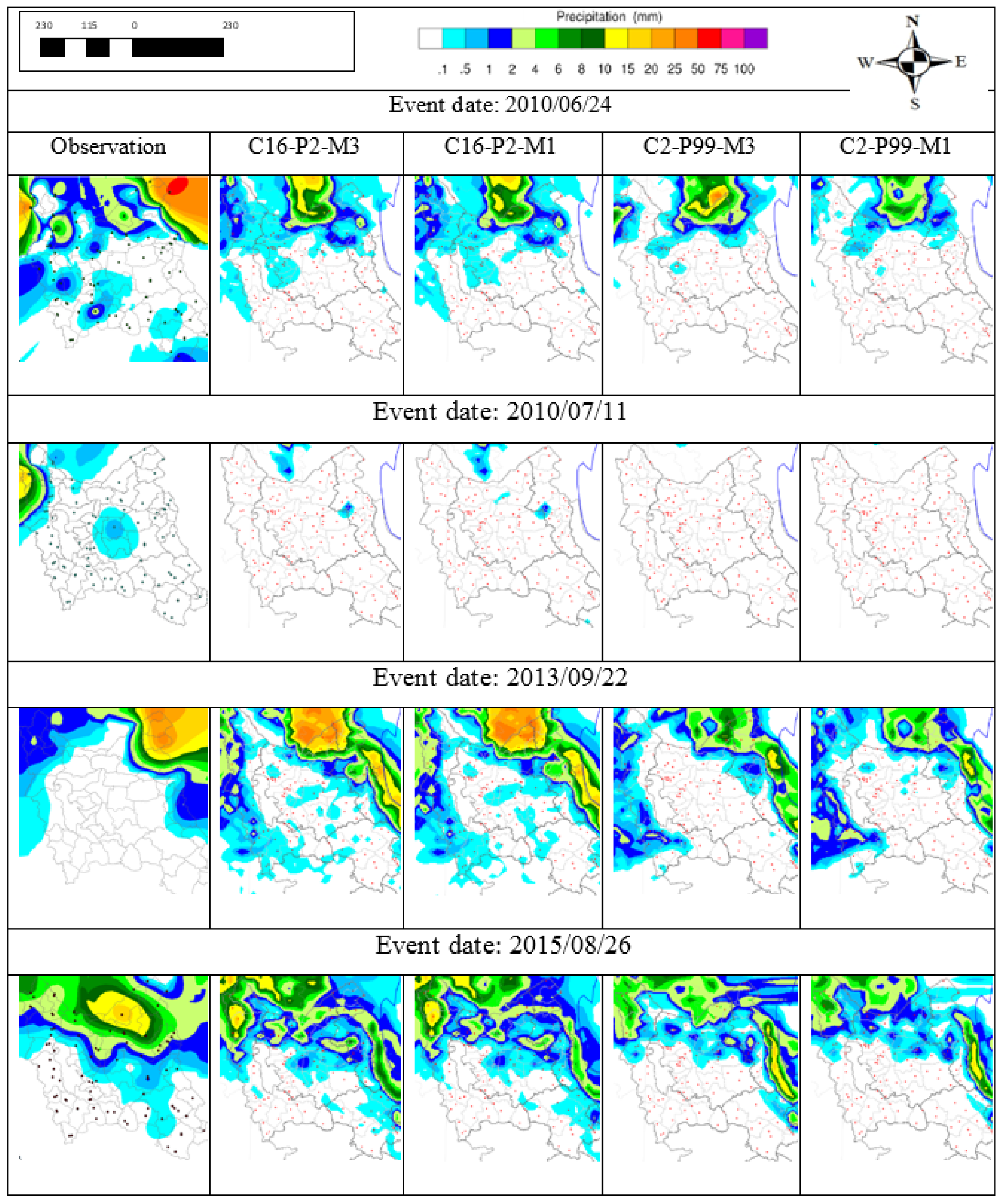
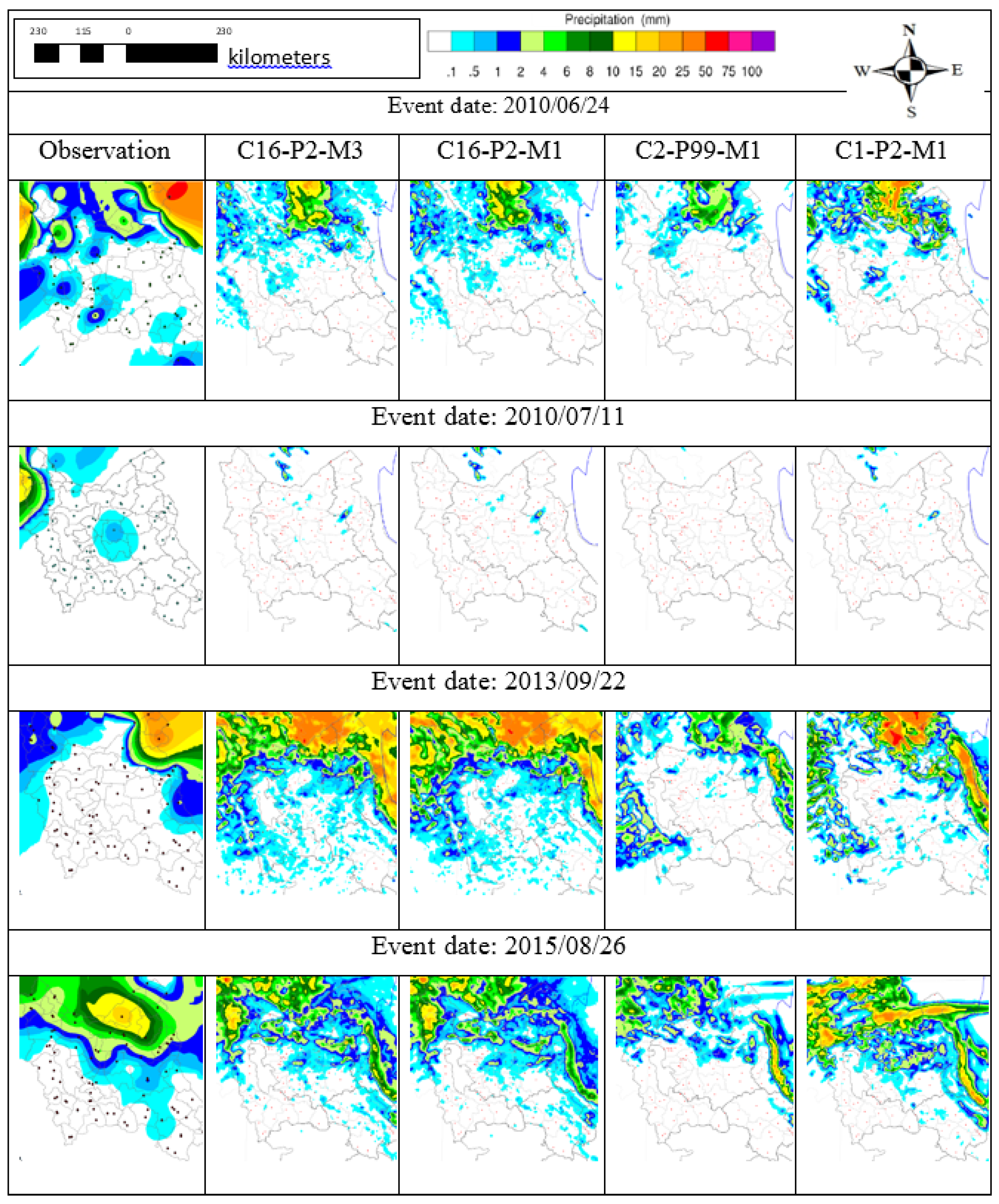
Finally, the results were checked by eyeball verification to identify the best model amongst the models selected by statistical methods. The output of these models was compared with observations obtained by interpolation with kriging in two resolutions (5 km & 15 km). Figure 4 and Figure 5 display the result of models and observation in four events. One of the oldest and best verification methods is the good old fashioned visual, or “eyeball”, method. Comparison the results, show that heavy rain in large area Conformity with the models, except of event on date of 7 November 2010. For example, Models C16-P2-M3 and C16-P2-M1 were simulated heavy rainfall in the upper right of area in event date 22 September 2013 in Figure 4. There is a clear difference in rainfall amount in the north central region between the c16 models and c2 models at 15 km resolution. It is shown c16 models are closer than c2 models to observations. Also, Figure 4, especially in event 26 August 2015, are shown that precipitation are simulated better by c16 models in the south central. Finally, comparing the model output images with map observations leads to a final decision on the best model. According to Figure 4 and Figure 5, models c16-p2-m1 and c16-p2-m3 show a very close similarity to the observations in both 5 and 15 km resolutions. They have used newer Tiedtke cumulus, Mellor-Yamada-Janjic PBL, WSM3 and Kessler microphysical schemes.
Since there are only 87 actual data points, the interpolated grid points are not all statistically independent of each other as there must be a spatial correlation between the interpolated points that is related to the average spacing of the original stations. It is suggested that in additional studies, radar data or more events can be used to more accurately control the models, then the comparison would be improved if the simulation data are interpolated to the station positions.
6. Conclusions
Most rainfalls in the Northwest of Iran in summer season are convective, with heavy rainfall occurring in some smaller areas. The results of verification by all of the methods clearly shows that NWP models cannot accurately predict this type of precipitation.
On the other hand, the result in Table 4 and Table 5 indicate that cumulus schemes are the most sensitive. Microphysical schemes are the least sensitive. This is also illustrated in the Taylor diagrams, in Figure 2 and Figure 3. In the Tayor diagrams, the models with the same cumulus and different PBL and microphysics show very similar outcomes. Comparison of 15-km resolution simulation with 5 km resolution simulation does not show obvious advantages, according to the verification score.
Configuration with the newer Tiedtke cumulus, Mellor-Yamada-Janjic PBL, WSM3 and Kessler microphysics schemes demonstrate the best results in both resolutions (5 and 15 km). There is little difference in the results between WSM3 and Kessler microphysics schemes. However, the results of WSM3 microphysics scheme are better than Kessler microphysical scheme.
No single configuration of the multi-physics performed best for all cases. In the first 24 h forecast of these 26 configurations, it has been observed, based on the output image of models and statistical methods, that convective rainfall in the NWI could not be simulated with high accuracy using WRF model in summer. This conclusion is based on statistical indexes and Eyeball verifications. Therefore, accuracy in the first 24 h forecast with the other methods needs to be improved. A method such as extrapolation of observation data using satellite and radar data can be used to improve forecast in first 24 h.
Acknowledgments
This work was supported by the Iran Atmospheric Science and Meteorological Research Center. Most of the data used in this research were collected from I.R. of Iran Meteorological Organization (IRIMO) and National Drought Warning and Monitoring Center (NDWMC) in Iran. We would like to thank all of those at these organizations, especially Director of NDWMC Shahrokh Fateh and President of IRIMO Davood Parhizkar.
Author Contributions
This paper is the result of research conducted by Sadegh Zeyaeyan as part of his PhD studies at the Atmospheric Science & Meteorological Research Center. Ebrahim Fattahi and Abbas Ranjbar jointly supervised and Majid Azadi and Majid Vazifedoust jointly advisor this project. Model running was conducted by Sadegh Zeyaeyan with guidance from Majid Azadi, Ebrahim Fattahi, Abbas Ranjbar and Majid Vazifedoust provided guidance on the analysis of the results. The manuscript was prepared by Sadegh Zeyaeyan with suggestions and corrections from Majid Azadi, Ebrahim Fattahi and Abbas Ranjbar. All authors have seen and approved the final article.
Conflicts of Interest
The authors declare no conflict of interest.
References
- Tohidi, A.; Ranjbar, A.; Meshqati, A.H. Investigation about Heavy Rains in West Azarbaijan Province in Spring and Determine the Atmospheric Circulation Pattern on That Rainfall; Islamic Azad University, Science and Research: Tehran, Iran, 2011. [Google Scholar]
- Easterling, D.R.; Gerald, A.M.; Camille, P.; Stanley, A.C.; Thomas, R.K.; Linda, O.M. Climate Extremes. Obs. Model. Impacts Sci. 2000, 289, 2068–2074. [Google Scholar]
- Manton, M.J.; Della-marta, P. M.; Haylock, M. R.; Hennessy, K. J.; Nicholls, N.; Chambers, L. E.; Collins, D.A.; Daw, G.; Finet, A.; Gunawan, D.; et al. Trend in Extreme Daily Rainfall and Temperature in Southeast Asia and South Pacific. Int. J. Clim. 2001, 21, 269–284. [Google Scholar] [CrossRef]
- Sura, P. Stochastic Models of Climate Extremes: Theory and Observations; Springer: Berlin/Heidelberg, Germany, 2012. [Google Scholar]
- Sheikh, M.M.; Ahmed, A.U.; Revadekar, J.V.; Shrestha, M.L.; Premlal, K.H.M.S. Development and Application of Climate Extreme Indices and Indicators for Monitoring Trends in Climate Extremes and Their Socio-Economic Impacts in South Asian Countries; Final Report for APN Project: ARCP2008-10CMY-Sheikh; APN: Kobe, Japan, 2009. [Google Scholar]
- Gholami, V.; Chau, K.W.; Fadaee, F.; Torkaman, J.; Ghaffari, A. Modeling of groundwater level fluctuations using dendrochronology in alluvial aquifers. J. Hydrol. 2015, 529, 1060–1069. [Google Scholar] [CrossRef]
- Taormina, R.; Chau, K.W. Data-driven input variable selection for rainfall-runoff modeling using binary-coded particle swarm optimization and Extreme Learning Machines. J. Hydrol. 2015, 529, 1617–1632. [Google Scholar] [CrossRef]
- Wang, W.C.; Chau, K.; Xu, D.M.; Chen, X.Y. Improving forecasting accuracy of annual runoff time series using ARIMA based on EEMD decomposition. Water Resour. Manag. 2015, 29, 2655–2675. [Google Scholar] [CrossRef]
- Chen, X.Y.; Chau, K.W.; Busari, A.O. A comparative study of population-based optimization algorithms for downstream river flow forecasting by a hybrid neural network model. Eng. Appl. Artif. Intell. 2015, 46, 258–268. [Google Scholar] [CrossRef]
- Chau, K.W.; Wu, C.L. A Hybrid Model Coupled with Singular Spectrum Analysis for Daily Rainfall Prediction. J. Hydroinform. 2010, 12, 458–473. [Google Scholar] [CrossRef]
- Wu, C.L.; Chau, K.W.; Fan, C. Prediction of rainfall time series using modular artificial neural networks coupled with data-preprocessing techniques. J. Hydrol. 2010, 389, 146–167. [Google Scholar] [CrossRef]
- Zeyaeyan, S.; Fattahi, E.; Ranjbar, A.; Vazifedoust, M. Classification of Rainfall Warning Based on the TOPSIS method. Climate 2017. [Google Scholar] [CrossRef]
- Evans, J.P.; Ekstrom, M.; Ji, F. Evaluating the performance of a WRF physics ensemble over South-East Australia. Clim. Dyn. 2011, 39, 1241–1258. [Google Scholar] [CrossRef]
- Rajeevan, M.; Kesarkar, A.; Thampi, S.B.; Rao, T.N.; Radhakrishna, B.; Rajasekhar, M. Sensitivity of WRF cloud microphysics to simulations of a severe thunderstorm event over Southeast India. Ann. Geophys. 2010, 28, 603–619. [Google Scholar] [CrossRef]
- Satyaban, B.; Ratnam, J.V.; Behera, S.K.; Rautenbach, C.J.D.; Ndarana, T.; Takahashi, K.; Yamagata, T. Performance assessment of three convective parameterization schemes in WRF for downscaling summer rainfall over South Africa. Clim. Dyn. 2013, 42, 2931–2953. [Google Scholar]
- Pennelly, C.; Reuter, G.; Flesch, T. Verification of the WRF model for simulating heavy precipitation in Alberta. Atmos. Res. 2014, 135, 172–192. [Google Scholar] [CrossRef]
- Li, L.F.; Li, W.H.; Jin, J.M. Improvements in WRF simulation skills of southeastern United States summer rainfall: physical parameterization and horizontal resolution. Clim. Dyn. 2014, 43, 7–8. [Google Scholar] [CrossRef]
- Chakrit, C.; Jiemjai, K.; Somporn, C. Evaluation of Precipitation Simulations over Thailand using a WRF Regional Climate Model. Chiang Mai J. Sci. Contrib. Pap. 2012, 39, 623–638. [Google Scholar]
- Hu, M.X.; Nielsen, G.; Zhang, F.Q. Evaluation of Three Planetary Boundary Layer Schemes in the WRF Model. Am. Meteorol. Soc. 2010, 49, 1831–1844. [Google Scholar] [CrossRef]
- Jankov, I.; Gallus, W. J.; Segal, M.; Shaw, B.; Koch, S. The impact of different WRF model physical parameterizations and their interactions on warm season MCS rainfall. Weather Forecast. 2005, 20, 1048–1060. [Google Scholar] [CrossRef]
- Jankov, I.; Schultz, P.; Anderson, C.; Koch, S. The impact of different physical parameterizations and their interactions on cold season QPF in the American River basin. J. Hydrometeorol. 2007, 8, 1141–1151. [Google Scholar] [CrossRef]
- Flaounas, E.; Bastin, S.; Janicot, S. Regional climate modelling of the 2006 West African monsoon sensitivity to convection and planetary boundary layer parameterisation using WRF. Clim. Dyn. 2011, 36, 1083–1105. [Google Scholar] [CrossRef]
- Barkovsky, M.; Karoly, D. Precipitation simulations using WRF as a nested regional climate model. Appl. Meteorol. Climatol. 2009, 48, 2152–2159. [Google Scholar] [CrossRef]
- Asakereh, H.; Ramzi, R. Climatology of Precipitation in North West of Iran. Geogr. Dev. 2012, 9, 137–158. [Google Scholar]
- Skamarock, W.C. A Description of the Advanced Research WRF Version 3; National Center for Atmospheric Research: Boulder, CO, USA, 2008. [Google Scholar]
- Berg, L.K.; Evgueni, I.K.; Gustafson, W.I., Jr.; Deng, L.P. Evaluation of a Modified Scheme for Shallow Convection: Implementation of CuP and Case Studies. Am. Meteorol. Soc. 2013, 141, 134–147. [Google Scholar] [CrossRef]
- WRF Users Page. 2016. Available online: http://www2.mmm.ucar.edu/wrf/users/wrfv3.8/updates-3.8.html (accessed on 8 November 2016).
- Wedi, N.P. Increasing horizontal resolution in numerical weather prediction and climate simulations: Illusion or panacea? Philosophical transactions of the royal society a mathematical. Phys. Eng. Sci. 2014. [Google Scholar] [CrossRef] [PubMed]
- Murphy, A.H.; Winkler, R.L. A General Framework for Forecast Verification. Mon. Weather Rev. 1987, 115, 1330–1338. [Google Scholar] [CrossRef]
- WWRP WCRP JWGFVR. World Weather Research Programme. Available online: http://www.cawcr.gov.au/projects/verification/#Introductio (accessed on 8 November 2016).
- Cressie, N.; Johannesson, G. Fixed rank kriging for very larg spatial data sets. J. R. Stat. Soc. Ser. B (Stat. Methodol.) 2008, 70, 209–226. [Google Scholar] [CrossRef]
- Sokal, R.R.; Rohlf, F.J. Biometry: The Principles and Practice of Statistics in, 3rd ed.; W. H. Freeman and Company: New York, NY, USA, 1995. [Google Scholar]
- McDonald, J.H. Handbook of Biological Statistics; Sparky House Publishing: Baltimore, MD, USA, 2014; p. 3. [Google Scholar]
- Finley, J.P. Tornado predictions. Am. Meteorol. J. 1884, 1, 85–88. [Google Scholar]
- Gilbert, G.F. Finley’s tornado predictions. Am. Meteorol. J. 1884, 4, 166–172. [Google Scholar]
- Stephenson, D.B. Use of the “Odds Ratio” for Diagnosing Forecast Skill. Weather Forecast. 1999, 15, 221–232. [Google Scholar] [CrossRef]
- Doolittle, M.H. The verification of predictions. Am. Meteorol. 1885, 7, 327–329. [Google Scholar]
- Heidke, P. Berechnung des Erfolges und der Gute der Windstarkevorhersagen im Sturmwarnungdienst (Calculation of the success and goodness of strong wind forecasts in the storm warning service). Geogr. Ann. Stockh. 1926, 8, 301–349. [Google Scholar]
- Peirce, C.S. The numerical measure of the success of predictions. Science 1884, 4, 453–454. [Google Scholar] [CrossRef] [PubMed]
- Hanssen, A.W.; Kuipers, W.J.A. On the relationship between the frequency of rain and various meteorological parameters. Meded. Verh. 1965, 47, 2–15. [Google Scholar]
- Schaefer, J.T. The critical success index as an indicator of warning skill. Weather Forecast. 1990, 5, 570–575. [Google Scholar] [CrossRef]
- Agresti, A. An Introduction to Categorical Data Analysis; John Wiley and Sons: New York, NY, USA, 1996. [Google Scholar]
- Yule, G.U. On the association of attributes in statistics. Philos. Trans. R. Lond. Philos. Trans. R. Soc. 1900, 194, 257–319. [Google Scholar] [CrossRef]
- Taylor, K.E. summarizing multiple aspects of model performance in a single diagram. J. Geophys. Res. 2001, 106, 7183–7192. [Google Scholar] [CrossRef]
- Houghton, J.T.; Ding, Y.; Griggs, D.J.; Noguer, N.; van der Linden, P.J.; Dai, X.; Maskell, K.; Johnson, C.A. Climate Change 2001: The Scientific Basis, Contribution of Working Group I to the Third Assessment Report of the Intergovernmental Panel on Climate Change; Cambridge University Press: Cambridge, UK; New York, NY, USA, 2001. [Google Scholar]
- Woodcock, F. The evaluation of yes/no forecasts for scientific and administrative purposes. Mon. Weather Rev. 1976, 104, 1209–1214. [Google Scholar] [CrossRef]
Figure 1.
The two domains of the study, 15 km and 5 km resolutions.
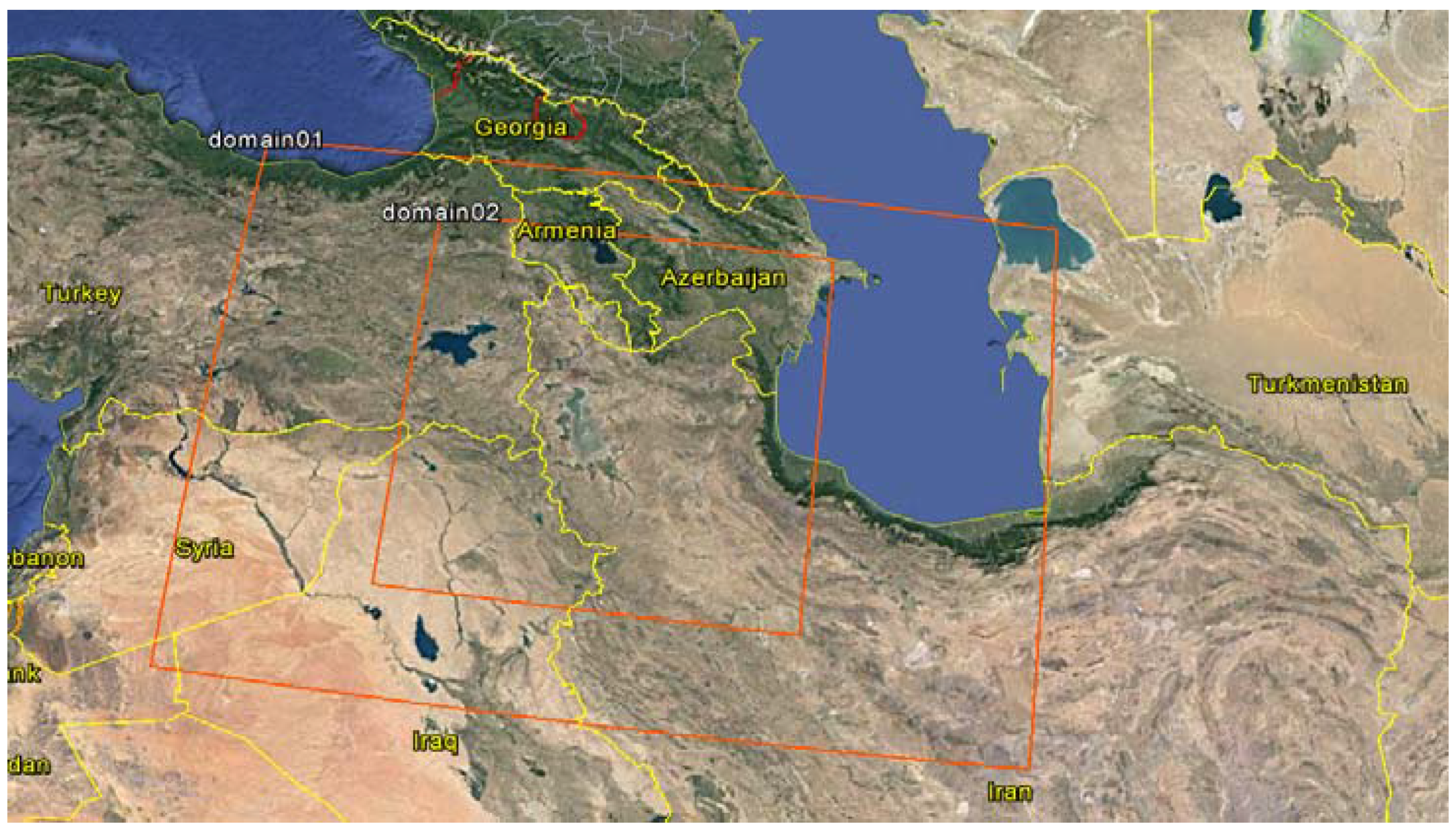
Figure 2.
Taylor diagram to verification models with 15 km resolution.
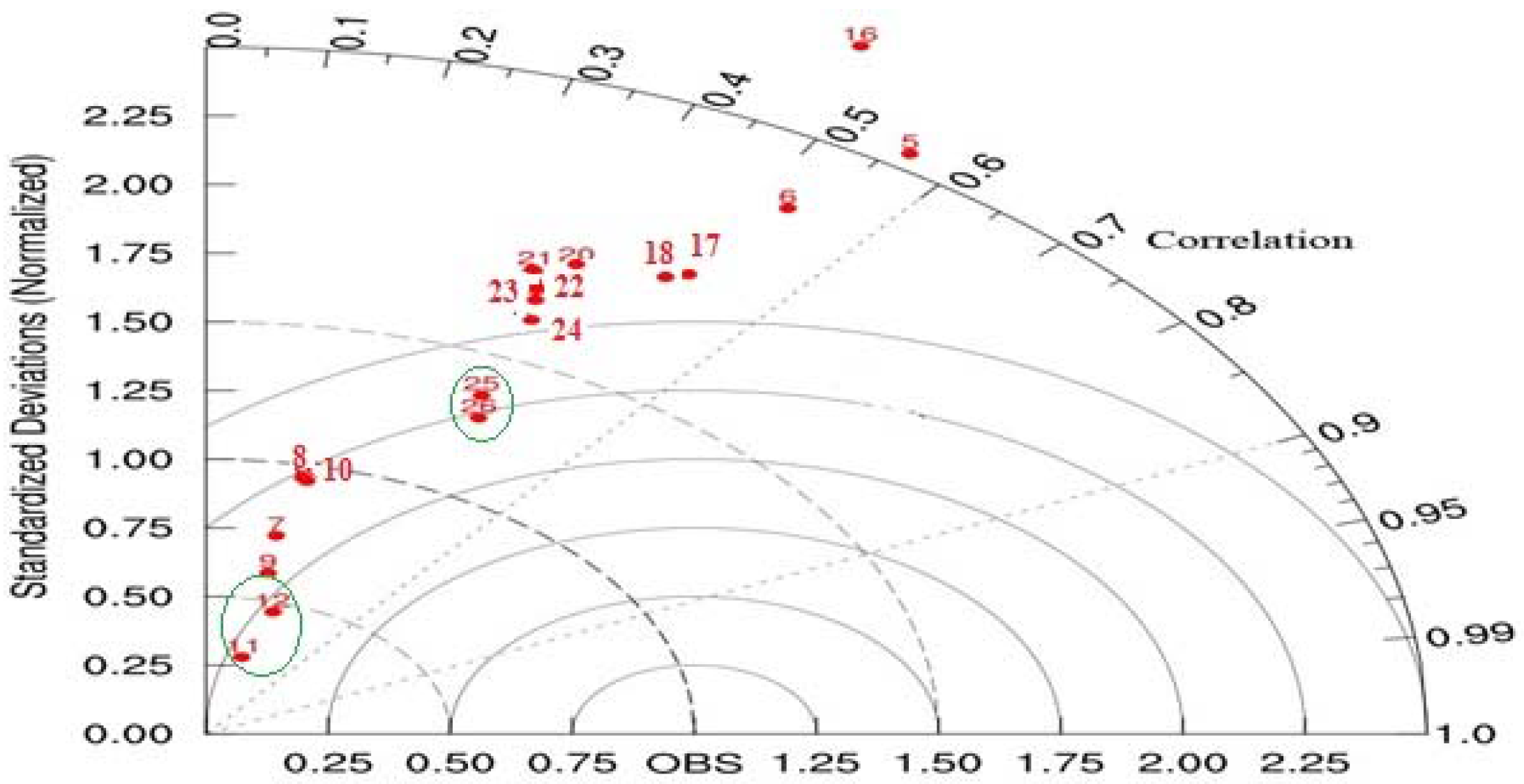
Figure 3.
Taylor diagram to verification models with 5 km resolution.
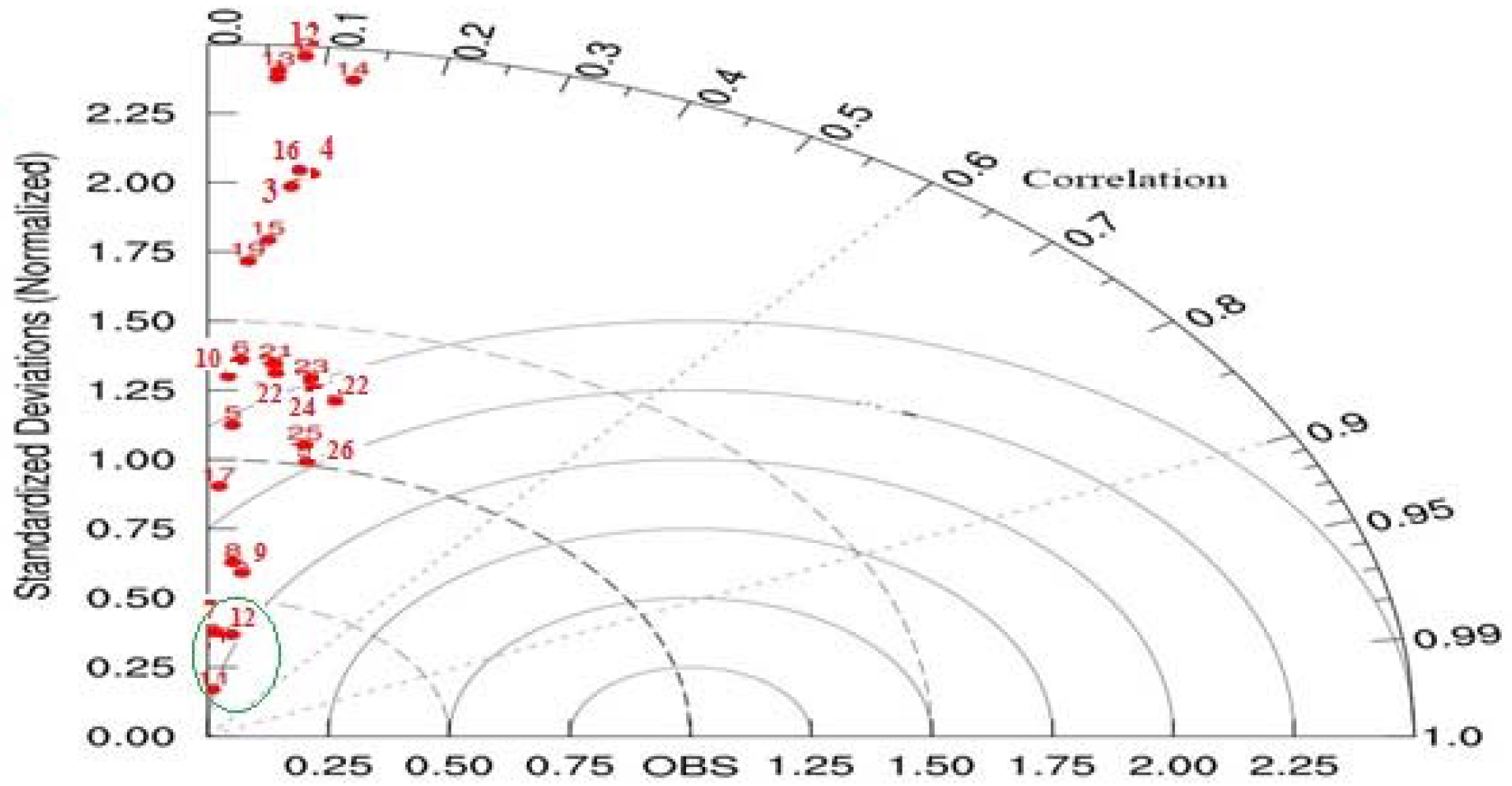
Figure 4.
Compare between models and observation (Eyeball verification), Resolution 15 km.

Figure 5.
Compare between models and observation (Eyeball verification), Resolution 5 km.


Table 1.
Schemes and different configuration.
| No | Cumulus Scheme | PBL Scheme | Microphysics Scheme | Number of Configuration |
|---|---|---|---|---|
| 1 | =1, Kain-Fritsch (new Eta) | =2, Mellor-Yamada-Janjic TKE | =1, Kessler | 4 × 3 × 2 = 24 |
| 2 | =2, Betts-Miller-Janjic | =11, Shin-Hong ‘scale-aware’ | =3, WSM 3-class simple ice | |
| 3 | =10, Modified Kain-Fritsch | =99, MRF | ||
| 4 | =16, A newer Tiedtke | |||
| 5 | =11, Multi-scale Kain-Fritsch | =1, YSU | =1, Kessler scheme | 1 × 1 × 2 = 2 |
| =3, WSM 3-class simple ice | ||||
| Total number of configuration | 26 | |||
Table 2.
Date of events.
| No | Date | ||
|---|---|---|---|
| Year | Month | Day | |
| 1 | 2010 | 6 | 24 |
| 2 | 2010 | 7 | 11 |
| 3 | 2013 | 9 | 22 |
| 4 | 2015 | 8 | 26 |
Table 3.
Latitude and longitude was used in domains.
| Point | Domain 1 | Domain 2 | ||
|---|---|---|---|---|
| Latitude | Longitude | Latitude | Longitude | |
| Lower left | 32°47′36.74″ N | 38°27′38.95″ E | 34°45′26.24″ N | 42°10′28.6″3 E |
| Upper left | 41°18′55.26″ N | 38°27′38.95″ E | 40°36′31.93″ N | 42°10′28.63″ E |
| Lower right | 32°47′36.74″ N | 53°57′42.55″ E | 34°45′26.2″4 N | 49°42′41.58″ E |
| Upper right | 41°18′55.26″ N | 53°5′742.55″ E | 40°363′1.93″ N | 49°42′41.58″ E |
Table 4.
Contingency table.
| Observed | ||||
|---|---|---|---|---|
| yes | No | Total | ||
| Forecast | Yes | a | B | forecast yes |
| No | c | D | forecast no | |
| Total | observed yes | observed no | n = a + b + c + d = total | |
a = event forecast to occur, and did occur; b = event forecast to occur, but did not occur; c = event forecast not to occur, but did occur, d = event forecast not to occur, and did not occur.
Table 5.
Verification results for a resolution of 15 km.
| No | Models | A | B | C | D | PC | TS | Odds Ratio | B | FAR | H | F | HSS | PSS | CSS | GSS | Q | RMSE |
|---|---|---|---|---|---|---|---|---|---|---|---|---|---|---|---|---|---|---|
| 1 | c1-p2-m1 | 920 | 621 | 351 | 717 | 0.63 | 0.49 | 3.026 | 1.21 | 0.4 | 0.72 | 0.46 | 0.26 | 0.26 | 0.27 | 0.15 | 0.5 | 8.07 |
| 2 | c1-p2-m3 | 937 | 636 | 334 | 702 | 0.63 | 0.49 | 3.097 | 1.24 | 0.4 | 0.74 | 0.48 | 0.26 | 0.26 | 0.27 | 0.15 | 0.51 | 7.11 |
| 3 | c1-p11-m1 | 882 | 588 | 389 | 750 | 0.63 | 0.47 | 2.892 | 1.16 | 0.4 | 0.69 | 0.44 | 0.25 | 0.25 | 0.26 | 0.15 | 0.49 | 7.56 |
| 4 | c1-p11-m3 | 899 | 602 | 372 | 736 | 0.63 | 0.48 | 2.955 | 1.18 | 0.4 | 0.71 | 0.45 | 0.26 | 0.26 | 0.26 | 0.15 | 0.49 | 6.76 |
| 5 | c1-p99-m1 | 815 | 512 | 456 | 826 | 0.63 | 0.46 | 2.883 | 1.04 | 0.39 | 0.64 | 0.38 | 0.26 | 0.26 | 0.26 | 0.15 | 0.49 | 5.95 |
| 6 | c1-p99-m3 | 833 | 520 | 438 | 818 | 0.63 | 0.47 | 2.992 | 1.07 | 0.38 | 0.66 | 0.39 | 0.27 | 0.27 | 0.27 | 0.15 | 0.5 | 5.61 |
| 7 | c2-p2-m1 | 892 | 584 | 379 | 754 | 0.63 | 0.48 | 3.039 | 1.16 | 0.4 | 0.7 | 0.44 | 0.26 | 0.27 | 0.27 | 0.15 | 0.51 | 3.23 |
| 8 | c2-p2-m3 | 894 | 589 | 377 | 749 | 0.63 | 0.48 | 3.016 | 1.17 | 0.4 | 0.7 | 0.44 | 0.26 | 0.26 | 0.27 | 0.15 | 0.5 | 3.73 |
| 9 | c2-p11-m1 | 875 | 561 | 396 | 777 | 0.63 | 0.48 | 3.06 | 1.13 | 0.39 | 0.69 | 0.42 | 0.27 | 0.27 | 0.27 | 0.16 | 0.51 | 2.88 |
| 10 | c2-p11-m3 | 881 | 562 | 390 | 776 | 0.64 | 0.48 | 3.119 | 1.14 | 0.39 | 0.69 | 0.42 | 0.27 | 0.27 | 0.28 | 0.16 | 0.51 | 3.66 |
| 11 | c2-p99-m1 | 815 | 485 | 456 | 853 | 0.64 | 0.46 | 3.143 | 1.02 | 0.37 | 0.64 | 0.36 | 0.28 | 0.28 | 0.28 | 0.16 | 0.52 | 1.96 |
| 12 | c2-p99-m3 | 798 | 487 | 473 | 851 | 0.63 | 0.45 | 2.948 | 1.01 | 0.38 | 0.63 | 0.36 | 0.26 | 0.26 | 0.26 | 0.15 | 0.49 | 2.5 |
| 13 | c10-p2-m1 | 925 | 604 | 346 | 734 | 0.64 | 0.49 | 3.249 | 1.2 | 0.4 | 0.73 | 0.45 | 0.28 | 0.28 | 0.29 | 0.16 | 0.53 | 7.11 |
| 14 | c10-p2-m3 | 931 | 625 | 340 | 713 | 0.63 | 0.49 | 3.124 | 1.22 | 0.4 | 0.73 | 0.47 | 0.26 | 0.27 | 0.28 | 0.15 | 0.52 | 6.75 |
| 15 | c10-p11-m1 | 890 | 583 | 381 | 755 | 0.63 | 0.48 | 3.025 | 1.16 | 0.4 | 0.7 | 0.44 | 0.26 | 0.27 | 0.27 | 0.15 | 0.5 | 6.76 |
| 16 | c10-p11-m3 | 898 | 604 | 373 | 734 | 0.63 | 0.48 | 2.926 | 1.18 | 0.4 | 0.71 | 0.45 | 0.25 | 0.26 | 0.26 | 0.15 | 0.49 | 6.41 |
| 17 | c10-p99-m1 | 804 | 513 | 467 | 825 | 0.62 | 0.45 | 2.769 | 1.04 | 0.39 | 0.63 | 0.38 | 0.25 | 0.25 | 0.25 | 0.14 | 0.47 | 5.16 |
| 18 | c10-p99-m3 | 818 | 505 | 453 | 833 | 0.63 | 0.46 | 2.979 | 1.04 | 0.38 | 0.64 | 0.38 | 0.27 | 0.27 | 0.27 | 0.15 | 0.5 | 5.15 |
| 19 | c16-p2-m1 | 973 | 631 | 298 | 707 | 0.64 | 0.51 | 3.658 | 1.26 | 0.39 | 0.77 | 0.47 | 0.29 | 0.29 | 0.31 | 0.17 | 0.57 | 5.19 |
| 20 | c16-p2-m3 | 980 | 641 | 291 | 697 | 0.64 | 0.51 | 3.662 | 1.28 | 0.4 | 0.77 | 0.48 | 0.29 | 0.29 | 0.31 | 0.17 | 0.57 | 5.09 |
| 21 | c16-p11-m1 | 951 | 627 | 320 | 711 | 0.64 | 0.5 | 3.37 | 1.24 | 0.4 | 0.75 | 0.47 | 0.28 | 0.28 | 0.29 | 0.16 | 0.54 | 5.02 |
| 22 | c16-p11-m3 | 951 | 632 | 320 | 706 | 0.64 | 0.5 | 3.32 | 1.25 | 0.4 | 0.75 | 0.47 | 0.27 | 0.28 | 0.29 | 0.16 | 0.54 | 4.89 |
| 23 | c16-p99-m1 | 931 | 610 | 340 | 728 | 0.64 | 0.5 | 3.268 | 1.21 | 0.4 | 0.73 | 0.46 | 0.28 | 0.28 | 0.29 | 0.16 | 0.53 | 4.39 |
| 24 | c16-p99-m3 | 933 | 609 | 338 | 729 | 0.64 | 0.5 | 3.304 | 1.21 | 0.4 | 0.73 | 0.46 | 0.28 | 0.28 | 0.29 | 0.16 | 0.54 | 4.25 |
| 25 | c11-p1-m1 | 887 | 576 | 384 | 762 | 0.63 | 0.48 | 3.056 | 1.15 | 0.39 | 0.7 | 0.43 | 0.27 | 0.27 | 0.27 | 0.15 | 0.51 | 6.47 |
| 26 | c11-p1-m3 | 898 | 592 | 373 | 746 | 0.63 | 0.48 | 3.034 | 1.17 | 0.4 | 0.71 | 0.44 | 0.26 | 0.26 | 0.27 | 0.15 | 0.5 | 5.17 |
Table 6.
Verification results for resolution of 5 km.
| No | Models | A | B | C | D | PC | TS | Odds Ratio | B | FAR | H | F | HSS | PSS | CSS | GSS | Q | RMSE |
|---|---|---|---|---|---|---|---|---|---|---|---|---|---|---|---|---|---|---|
| 1 | c1-p2-m1 | 5945 | 2779 | 4708 | 6100 | 0.617 | 0.443 | 2.772 | 0.819 | 0.319 | 0.558 | 0.313 | 0.241 | 0.245 | 0.246 | 0.137 | 0.470 | 5.87 |
| 2 | c1-p2-m3 | 6099 | 3053 | 4554 | 5826 | 0.611 | 0.445 | 2.556 | 0.859 | 0.334 | 0.573 | 0.344 | 0.225 | 0.229 | 0.228 | 0.127 | 0.438 | 5.99 |
| 3 | c1-p11-m1 | 5162 | 2513 | 5491 | 6366 | 0.590 | 0.392 | 2.381 | 0.720 | 0.327 | 0.485 | 0.283 | 0.196 | 0.202 | 0.209 | 0.109 | 0.409 | 5.34 |
| 4 | c1-p11-m3 | 5519 | 2720 | 5134 | 6159 | 0.598 | 0.413 | 2.434 | 0.773 | 0.330 | 0.518 | 0.306 | 0.207 | 0.212 | 0.215 | 0.115 | 0.418 | 5.42 |
| 5 | c1-p99-m1 | 3967 | 2029 | 6686 | 6850 | 0.554 | 0.313 | 2.003 | 0.563 | 0.338 | 0.372 | 0.229 | 0.138 | 0.144 | 0.168 | 0.074 | 0.334 | 4.02 |
| 6 | c1-p99-m3 | 4312 | 2214 | 6341 | 6665 | 0.562 | 0.335 | 2.047 | 0.613 | 0.339 | 0.405 | 0.249 | 0.150 | 0.155 | 0.173 | 0.081 | 0.344 | 4.41 |
| 7 | c2-p2-m1 | 5928 | 3005 | 4725 | 5874 | 0.604 | 0.434 | 2.452 | 0.839 | 0.336 | 0.556 | 0.338 | 0.215 | 0.218 | 0.218 | 0.120 | 0.421 | 2.34 |
| 8 | c2-p2-m3 | 6102 | 3111 | 4551 | 5768 | 0.608 | 0.443 | 2.486 | 0.865 | 0.338 | 0.573 | 0.350 | 0.219 | 0.222 | 0.221 | 0.123 | 0.426 | 3 |
| 9 | c2-p11-m1 | 5488 | 2731 | 5165 | 6148 | 0.596 | 0.410 | 2.392 | 0.772 | 0.332 | 0.515 | 0.308 | 0.203 | 0.208 | 0.211 | 0.113 | 0.410 | 2.21 |
| 10 | c2-p11-m3 | 5578 | 2785 | 5075 | 6094 | 0.598 | 0.415 | 2.405 | 0.785 | 0.333 | 0.524 | 0.314 | 0.206 | 0.210 | 0.213 | 0.115 | 0.413 | 2.92 |
| 11 | c2-p99-m1 | 4261 | 2079 | 6392 | 6800 | 0.566 | 0.335 | 2.180 | 0.595 | 0.328 | 0.400 | 0.234 | 0.159 | 0.166 | 0.188 | 0.087 | 0.371 | 1.75 |
| 12 | c2-p99-m3 | 4540 | 2247 | 6113 | 6632 | 0.572 | 0.352 | 2.192 | 0.637 | 0.331 | 0.426 | 0.253 | 0.167 | 0.173 | 0.189 | 0.091 | 0.373 | 2.35 |
| 13 | c10-p2-m1 | 5572 | 2636 | 5081 | 6243 | 0.605 | 0.419 | 2.597 | 0.770 | 0.321 | 0.523 | 0.297 | 0.221 | 0.226 | 0.230 | 0.124 | 0.444 | 5.88 |
| 14 | c10-p2-m3 | 5977 | 2995 | 4676 | 5884 | 0.607 | 0.438 | 2.511 | 0.842 | 0.334 | 0.561 | 0.337 | 0.220 | 0.224 | 0.223 | 0.124 | 0.430 | 5.89 |
| 15 | c10-p11-m1 | 5027 | 2422 | 5626 | 6457 | 0.588 | 0.384 | 2.382 | 0.699 | 0.325 | 0.472 | 0.273 | 0.193 | 0.199 | 0.209 | 0.107 | 0.409 | 5.06 |
| 16 | c10-p11-m3 | 5415 | 2733 | 5238 | 6146 | 0.592 | 0.405 | 2.325 | 0.765 | 0.335 | 0.508 | 0.308 | 0.196 | 0.201 | 0.204 | 0.109 | 0.398 | 5.41 |
| 17 | c10-p99-m1 | 3727 | 1957 | 6926 | 6922 | 0.545 | 0.296 | 1.903 | 0.534 | 0.344 | 0.350 | 0.220 | 0.124 | 0.129 | 0.156 | 0.066 | 0.311 | 3.63 |
| 18 | c10-p99-m3 | 4151 | 2188 | 6502 | 6691 | 0.555 | 0.323 | 1.952 | 0.595 | 0.345 | 0.390 | 0.246 | 0.138 | 0.143 | 0.162 | 0.074 | 0.323 | 4.31 |
| 19 | c16-p2-m1 | 6869 | 3664 | 3784 | 5215 | 0.619 | 0.480 | 2.584 | 0.989 | 0.348 | 0.645 | 0.413 | 0.232 | 0.232 | 0.232 | 0.131 | 0.442 | 4.4 |
| 20 | c16-p2-m3 | 6852 | 3656 | 3801 | 5223 | 0.618 | 0.479 | 2.575 | 0.986 | 0.348 | 0.643 | 0.412 | 0.231 | 0.231 | 0.231 | 0.131 | 0.441 | 4.34 |
| 21 | c16-p11-m1 | 6505 | 3413 | 4148 | 5466 | 0.613 | 0.462 | 2.512 | 0.931 | 0.344 | 0.611 | 0.384 | 0.225 | 0.226 | 0.224 | 0.127 | 0.430 | 4.33 |
| 22 | c16-p11-m3 | 6485 | 3359 | 4168 | 5520 | 0.615 | 0.463 | 2.557 | 0.924 | 0.341 | 0.609 | 0.378 | 0.229 | 0.230 | 0.229 | 0.129 | 0.438 | 4.27 |
| 23 | c16-p99-m1 | 5922 | 3257 | 4731 | 5622 | 0.591 | 0.426 | 2.161 | 0.862 | 0.355 | 0.556 | 0.367 | 0.187 | 0.189 | 0.188 | 0.103 | 0.367 | 3.91 |
| 24 | c16-p99-m3 | 5918 | 3242 | 4735 | 5637 | 0.592 | 0.426 | 2.173 | 0.860 | 0.354 | 0.556 | 0.365 | 0.188 | 0.190 | 0.190 | 0.104 | 0.370 | 3.8 |
| 25 | c11-p1-m1 | 5292 | 2658 | 5361 | 6221 | 0.589 | 0.398 | 2.310 | 0.746 | 0.334 | 0.497 | 0.299 | 0.193 | 0.197 | 0.203 | 0.107 | 0.396 | 4.95 |
| 26 | c11-p1-m3 | 5683 | 2929 | 4970 | 5950 | 0.596 | 0.418 | 2.323 | 0.808 | 0.340 | 0.533 | 0.330 | 0.200 | 0.204 | 0.205 | 0.111 | 0.398 | 4.2 |
Table 7.
Scoring the best results for verification methods 15 km resolution.
| No | Models | A | B | C | D | PC | TS | Odds Ratio | B | FAR | H | F | HSS | PSS | CSS | GSS | Q | RMSE | Taylor Diagram | Total Score |
|---|---|---|---|---|---|---|---|---|---|---|---|---|---|---|---|---|---|---|---|---|
| 1 | c1-p2-m1 | 0 | 0 | 0 | 0 | 0 | 0 | 0 | 0 | 0 | 0 | 0 | 0 | 0 | 0 | 0 | 0 | 0 | 0 | 0 |
| 2 | c1-p2-m3 | 0 | 0 | 0 | 0 | 0 | 0 | 0 | 0 | 0 | 0 | 0 | 0 | 0 | 0 | 0 | 0 | 0 | 0 | 0 |
| 3 | c1-p11-m1 | 0 | 0 | 0 | 0 | 0 | 0 | 0 | 0 | 0 | 0 | 0 | 0 | 0 | 0 | 0 | 0 | 0 | 0 | 0 |
| 4 | c1-p11-m3 | 0 | 0 | 0 | 0 | 0 | 0 | 0 | 0 | 0 | 0 | 0 | 0 | 0 | 0 | 0 | 0 | 0 | 0 | 0 |
| 5 | c1-p99-m1 | 0 | 0 | 0 | 0 | 0 | 0 | 0 | 0 | 0 | 0 | 0 | 0 | 0 | 0 | 0 | 0 | 0 | 0 | 0 |
| 6 | c1-p99-m3 | 0 | 0 | 0 | 0 | 0 | 0 | 0 | 0 | 0 | 0 | 0 | 0 | 0 | 0 | 0 | 0 | 0 | 0 | 0 |
| 7 | c2-p2-m1 | 0 | 0 | 0 | 0 | 0 | 0 | 0 | 0 | 0 | 0 | 0 | 0 | 0 | 0 | 0 | 0 | 0 | 0 | 0 |
| 8 | c2-p2-m3 | 0 | 0 | 0 | 0 | 0 | 0 | 0 | 0 | 0 | 0 | 0 | 0 | 0 | 0 | 0 | 0 | 0 | 0 | 0 |
| 9 | c2-p11-m1 | 0 | 0 | 0 | 0 | 0 | 0 | 0 | 0 | 0 | 0 | 0 | 0 | 0 | 0 | 0 | 0 | 0 | 0 | 0 |
| 10 | c2-p11-m3 | 0 | 0 | 0 | 0 | 0 | 0 | 0 | 0 | 0 | 0 | 0 | 0 | 0 | 0 | 0 | 0 | 0 | 0 | 0 |
| 11 | c2-p99-m1 | 0 | 1 | 0 | 1 | 0 | 0 | 0 | 1 | 1 | 0 | 1 | 0 | 0 | 0 | 0 | 0 | 1 | 1 | 7 |
| 12 | c2-p99-m3 | 0 | 1 | 0 | 1 | 0 | 0 | 0 | 1 | 1 | 0 | 1 | 0 | 0 | 0 | 0 | 0 | 1 | 1 | 7 |
| 13 | c10-p2-m1 | 0 | 0 | 0 | 0 | 0 | 0 | 0 | 0 | 0 | 0 | 0 | 0 | 0 | 0 | 0 | 0 | 0 | 0 | 0 |
| 14 | c10-p2-m3 | 0 | 0 | 0 | 0 | 0 | 0 | 0 | 0 | 0 | 0 | 0 | 0 | 0 | 0 | 0 | 0 | 0 | 0 | 0 |
| 15 | c10-p11-m1 | 0 | 0 | 0 | 0 | 0 | 0 | 0 | 0 | 0 | 0 | 0 | 0 | 0 | 0 | 0 | 0 | 0 | 0 | 0 |
| 16 | c10-p11-m3 | 0 | 0 | 0 | 0 | 0 | 0 | 0 | 0 | 0 | 0 | 0 | 0 | 0 | 0 | 0 | 0 | 0 | 0 | 0 |
| 17 | c10-p99-m1 | 0 | 0 | 0 | 0 | 0 | 0 | 0 | 0 | 0 | 0 | 0 | 0 | 0 | 0 | 0 | 0 | 0 | 1 | 1 |
| 18 | c10-p99-m3 | 0 | 0 | 0 | 0 | 0 | 0 | 0 | 0 | 0 | 0 | 0 | 0 | 0 | 0 | 0 | 0 | 0 | 1 | 1 |
| 19 | c16-p2-m1 | 1 | 0 | 1 | 0 | 1 | 1 | 1 | 0 | 0 | 1 | 0 | 1 | 1 | 1 | 1 | 1 | 0 | 0 | 11 |
| 20 | c16-p2-m3 | 1 | 0 | 1 | 0 | 1 | 1 | 1 | 0 | 0 | 1 | 0 | 1 | 1 | 1 | 1 | 1 | 0 | 0 | 11 |
| 21 | c16-p11-m1 | 0 | 0 | 0 | 0 | 0 | 0 | 0 | 0 | 0 | 0 | 0 | 0 | 0 | 0 | 0 | 0 | 0 | 0 | 0 |
| 22 | c16-p11-m3 | 0 | 0 | 0 | 0 | 0 | 0 | 0 | 0 | 0 | 0 | 0 | 0 | 0 | 0 | 0 | 0 | 0 | 0 | 0 |
| 23 | c16-p99-m1 | 0 | 0 | 0 | 0 | 0 | 0 | 0 | 0 | 0 | 0 | 0 | 0 | 0 | 0 | 0 | 0 | 0 | 0 | 0 |
| 24 | c16-p99-m3 | 0 | 0 | 0 | 0 | 0 | 0 | 0 | 0 | 0 | 0 | 0 | 0 | 0 | 0 | 0 | 0 | 0 | 0 | 0 |
| 25 | c11-p1-m1 | 0 | 0 | 0 | 0 | 0 | 0 | 0 | 0 | 0 | 0 | 0 | 0 | 0 | 0 | 0 | 0 | 0 | 1 | 1 |
| 26 | c11-p1-m3 | 0 | 0 | 0 | 0 | 0 | 0 | 0 | 0 | 0 | 0 | 0 | 0 | 0 | 0 | 0 | 0 | 0 | 1 | 1 |
Table 8.
Scoring the best results for verification methods 5 km resolution.
| No | Models | A | B | C | D | PC | TS | Odds Ratio | B | FAR | H | F | HSS | PSS | CSS | GSS | Q | RMSE | Taylor Diagram | Total Score |
|---|---|---|---|---|---|---|---|---|---|---|---|---|---|---|---|---|---|---|---|---|
| 1 | c1-p2-m1 | 0 | 0 | 0 | 0 | 0 | 0 | 1 | 0 | 1 | 0 | 0 | 1 | 1 | 1 | 1 | 1 | 0 | 0 | 7 |
| 2 | c1-p2-m3 | 0 | 0 | 0 | 0 | 0 | 0 | 0 | 0 | 0 | 0 | 0 | 0 | 0 | 0 | 0 | 0 | 0 | 0 | 0 |
| 3 | c1-p11-m1 | 0 | 0 | 0 | 0 | 0 | 0 | 0 | 0 | 0 | 0 | 0 | 0 | 0 | 0 | 0 | 0 | 0 | 0 | 0 |
| 4 | c1-p11-m3 | 0 | 0 | 0 | 0 | 0 | 0 | 0 | 0 | 0 | 0 | 0 | 0 | 0 | 0 | 0 | 0 | 0 | 0 | 0 |
| 5 | c1-p99-m1 | 0 | 1 | 0 | 1 | 0 | 0 | 0 | 0 | 0 | 0 | 1 | 0 | 0 | 0 | 0 | 0 | 0 | 0 | 3 |
| 6 | c1-p99-m3 | 0 | 0 | 0 | 0 | 0 | 0 | 0 | 0 | 0 | 0 | 0 | 0 | 0 | 0 | 0 | 0 | 0 | 0 | 0 |
| 7 | c2-p2-m1 | 0 | 0 | 0 | 0 | 0 | 0 | 0 | 0 | 0 | 0 | 0 | 0 | 0 | 0 | 0 | 0 | 0 | 0 | 0 |
| 8 | c2-p2-m3 | 0 | 0 | 0 | 0 | 0 | 0 | 0 | 0 | 0 | 0 | 0 | 0 | 0 | 0 | 0 | 0 | 0 | 0 | 0 |
| 9 | c2-p11-m1 | 0 | 0 | 0 | 0 | 0 | 0 | 0 | 0 | 0 | 0 | 0 | 0 | 0 | 0 | 0 | 0 | 1 | 0 | 1 |
| 10 | c2-p11-m3 | 0 | 0 | 0 | 0 | 0 | 0 | 0 | 0 | 0 | 0 | 0 | 0 | 0 | 0 | 0 | 0 | 0 | 0 | 0 |
| 11 | c2-p99-m1 | 0 | 0 | 0 | 0 | 0 | 0 | 0 | 0 | 0 | 0 | 0 | 0 | 0 | 0 | 0 | 0 | 1 | 1 | 2 |
| 12 | c2-p99-m3 | 0 | 0 | 0 | 0 | 0 | 0 | 0 | 0 | 0 | 0 | 0 | 0 | 0 | 0 | 0 | 0 | 0 | 0 | 0 |
| 13 | c10-p2-m1 | 0 | 0 | 0 | 0 | 0 | 0 | 1 | 0 | 1 | 0 | 0 | 0 | 0 | 0 | 0 | 1 | 0 | 0 | 3 |
| 14 | c10-p2-m3 | 0 | 0 | 0 | 0 | 0 | 0 | 0 | 0 | 0 | 0 | 0 | 0 | 0 | 0 | 0 | 0 | 0 | 0 | 0 |
| 15 | c10-p11-m1 | 0 | 0 | 0 | 0 | 0 | 0 | 0 | 0 | 0 | 0 | 0 | 0 | 0 | 0 | 0 | 0 | 0 | 0 | 0 |
| 16 | c10-p11-m3 | 0 | 0 | 0 | 0 | 0 | 0 | 0 | 0 | 0 | 0 | 0 | 0 | 0 | 0 | 0 | 0 | 0 | 0 | 0 |
| 17 | c10-p99-m1 | 0 | 1 | 0 | 1 | 0 | 0 | 0 | 0 | 0 | 0 | 1 | 0 | 0 | 0 | 0 | 0 | 0 | 0 | 3 |
| 18 | c10-p99-m3 | 0 | 0 | 0 | 0 | 0 | 0 | 0 | 0 | 0 | 0 | 0 | 0 | 0 | 0 | 0 | 0 | 0 | 0 | 0 |
| 19 | c16-p2-m1 | 1 | 0 | 1 | 0 | 1 | 1 | 0 | 1 | 0 | 1 | 0 | 1 | 1 | 1 | 1 | 0 | 0 | 0 | 9 |
| 20 | c16-p2-m3 | 1 | 0 | 1 | 0 | 1 | 1 | 0 | 1 | 0 | 1 | 0 | 0 | 0 | 0 | 0 | 0 | 0 | 0 | 6 |
| 21 | c16-p11-m1 | 0 | 0 | 0 | 0 | 0 | 0 | 0 | 0 | 0 | 0 | 0 | 0 | 0 | 0 | 0 | 0 | 0 | 0 | 0 |
| 22 | c16-p11-m3 | 0 | 0 | 0 | 0 | 0 | 0 | 0 | 0 | 0 | 0 | 0 | 0 | 0 | 0 | 0 | 0 | 0 | 0 | 0 |
| 23 | c16-p99-m1 | 0 | 0 | 0 | 0 | 0 | 0 | 0 | 0 | 0 | 0 | 0 | 0 | 0 | 0 | 0 | 0 | 0 | 0 | 0 |
| 24 | c16-p99-m3 | 0 | 0 | 0 | 0 | 0 | 0 | 0 | 0 | 0 | 0 | 0 | 0 | 0 | 0 | 0 | 0 | 0 | 0 | 0 |
| 25 | c11-p1-m1 | 0 | 0 | 0 | 0 | 0 | 0 | 0 | 0 | 0 | 0 | 0 | 0 | 0 | 0 | 0 | 0 | 0 | 1 | 1 |
| 26 | c11-p1-m3 | 0 | 0 | 0 | 0 | 0 | 0 | 0 | 0 | 0 | 0 | 0 | 0 | 0 | 0 | 0 | 0 | 0 | 1 | 1 |
© 2017 by the authors. Licensee MDPI, Basel, Switzerland. This article is an open access article distributed under the terms and conditions of the Creative Commons Attribution (CC BY) license (http://creativecommons.org/licenses/by/4.0/).
Share and Cite
MDPI and ACS Style
Zeyaeyan, S.; Fattahi, E.; Ranjbar, A.; Azadi, M.; Vazifedoust, M. Evaluating the Effect of Physics Schemes in WRF Simulations of Summer Rainfall in North West Iran. Climate 2017, 5, 48. https://doi.org/10.3390/cli5030048
AMA Style
Zeyaeyan S, Fattahi E, Ranjbar A, Azadi M, Vazifedoust M. Evaluating the Effect of Physics Schemes in WRF Simulations of Summer Rainfall in North West Iran. Climate. 2017; 5(3):48. https://doi.org/10.3390/cli5030048
Chicago/Turabian StyleZeyaeyan, Sadegh, Ebrahim Fattahi, Abbas Ranjbar, Majid Azadi, and Majid Vazifedoust. 2017. "Evaluating the Effect of Physics Schemes in WRF Simulations of Summer Rainfall in North West Iran" Climate 5, no. 3: 48. https://doi.org/10.3390/cli5030048
Note that from the first issue of 2016, this journal uses article numbers instead of page numbers. See further details here.