
On the Use of Regression Models to Predict Tea Crop Yield Responses to Climate Change: A Case of Nandi East, Sub-County of Nandi County, Kenya


1
Department of Meteorology, University of Nairobi, P.O. Box 30197-00100 Nairobi, Kenya
2
Department of Mathematics, Kibabii University, P.O. BOX 1699-50200 Bungoma, Kenya
*
Author to whom correspondence should be addressed.
Climate 2017, 5(3), 54; https://doi.org/10.3390/cli5030054
Submission received: 21 June 2017
/
Revised: 4 July 2017
/
Accepted: 6 July 2017
/
Published: 17 July 2017
Abstract
:Tea is a major cash crop in Kenya. Predicting the potential effects of climate change on tea crops prompts the use of statistical models to measure how the crop responds to climate variables. The statistical model was trained on historical tea yields, and how they related to past data on maximum temperature, minimum temperature and precipitation over Nandi East Sub-County. Scatter diagrams for selected months were generated from tea yield and temperature data. A multiple linear model was developed to predict tea yield using climatic variables. A contingency table was used to verify the model. Results from an analysis of trends in rainfall depicted a positive trend and revealed an increased frequency of annual droughts. The study showed that the frequency of extreme rainfall events during September-October-November (SON) season has decreased. Results from an analysis of the trends in temperature revealed that the minimum temperatures are increasing and that the frequency of extreme events has increased. Rising maximum temperatures were observed in March. The study revealed that May, the cold month, is becoming warmer. Correlation analysis indicated that the climatic variables during some months in both the concurrent year and the previous year were positively correlated with the tea yield. However, there was an inverse relationship between maximum temperature and rainfall. Results of model verification revealed that that 70% of model forecasts were correct. The results also showed that at least half of the observed events were correctly forecasted and thus the majority of the forecasts were true. An equation for predicting the yield of tea from the climate variables is presented.
1. Introduction
1.1. Study Background
According to the recently released report of the Intergovernmental Panel on Climate Change (IPCC), it is certain that the global mean surface temperature of the earth has increased since the beginning of the instrumental record. This warming has been about 0.85 °C from 1880 to 2012, with an increase of about 0.72 °C from 1951 to 2012. Each of the last three decades has successively been the warmest on record. They also have very likely been the warmest in the last 800 years and likely the warmest in the last 1400 years, even if the rate of warming over the last 15 years is smaller than the rate since the 1950s [1].
According to Future Climate for Africa (FCSA) information on climate [2], tea and coffee crops are vulnerable to climate variability and change. They grow in subtropical to temperate, wet conditions, but the plants can be damaged by unseasonably heavy rains, or harmed by pests and diseases that spread in a changing climate. According to [3]), tea is planted in 58 countries across five continents, with Asia having the largest area under tea, followed by Africa [3].The total land under tea cultivation was 3.36 million hectares, and production in 2012 was 4.78 million tonnes [3]. Importantly, the size of land required to produce one unit of tea varies across countries. For instance, China produced 1.4 million tonnes of tea in 2011 under an estimated one million hectares of land (average yield of 1.4 tonnes per hectare), while India produced one million tonnes under 0.5 million hectares (2 tonnes per hectare). Despite recent growth trends, tea areas have not increased proportionately, except in China, implying an increase in global crop yields. However, there has been evidence of fluctuating yields, including several wild swings most likely due to climate change, particularly in Kenya. An explanation that has been put forward is that the expansion in area is due to the increase in number of organic tea farms with lower yields compared to conventional tea [4].
Studies by [5] investigated the use of statistical models in predicting maize crop yield. A perfect model approach was used to examine the ability of statistical models to predict yield responses to changes in mean temperature and precipitation, as simulated by a process-based crop model. Results of the study suggested that statistical models, as compared to Crop Environment Resource Synthesis (CERES) model applied to Maize crop (CERES-MAIZE) represented a useful tool for projecting future yield responses, with their usefulness higher at broader spatial scales. It was also noted that at these broader scales, climate projections were most available and reliable, and therefore statistical models were likely to continue to play an important role in anticipating future impacts of climate change. Lobell et al. [6] also investigated the relationship between wheat yield and climate trends in Mexico. They used a combination of mechanistic and statistical models to show that much of the yield increase could be attributed to climatic trends in northwest states, particularly the cooling of growing season nighttime temperatures. A similar study by [7] investigated the non-linear effects of African maize as evidenced by historical yield trials. A nonlinear relationship between warming and yield was observed. A similar study was also carried out on the impacts of future climate change on California perennial crop yields [7].The study revealed that despite uncertainties, climate change in California is very likely to put downward pressure on yields of almonds, walnuts, avocados, and table grapes by 2050. Kleijnen [8] cites the use of regression approaches to verify the performance and accuracy of statistical models. Kleijnen [9] also details verification statistics for regression models. Studies by [10] used contingency tables in quantitative precipitation forecasts over Australia. In this study, real-time gridded 24 h quantitative precipitation forecasts from seven operational Numerical Weather Prediction (NWP ) models were successfully verified over the Australian continent.
Studies by [11] used a multiple regression model of wheat yield response to environment. The model was tested against the independent data in one third of the data set (246 aggregated yield observations) and showed predictive power with a Pearson’s correlation coefficient (r) of r = 0.41, which was improved when comparing against mean annual yields (r = 0.77). The final model allowed the relative importance of the 17 explanatory variables, and the weather effects they represented (defined before fitting), to be assessed. The most important weather effects were found to be: (1) negative effects from rainfall on agronomy before and during anthesis, during grain filling, and in the spring; (2) winter frost damage; (3) a positive effect from the temperature-driven duration of grain filling; and (4) a positive effect from radiation around anthesis, probably due to increased photosynthesis. However, the model could not be used outside the United Kingdom. Tao et al. [12] carried out a study on climate–crop yield relationships at provincial scales in China, which measured the impacts of recent climate trends. The study found that major crop yields were significantly related to the growing season climate in the main production regions of China, and that growing season temperature had a generally significant warming trend. Due to the trends in the growing season climate, total rice production in China was estimated to have increased by 3.2 × 10⁵ t decade−1 during the period 1951–2002; total production of wheat, maize and soybean changed by −1.2 × 10⁵, −21.2 × 10⁵ and 0.7 × 10⁵ t decade−1, respectively, during 1979–2002. The warming trend increased rice yield in northeast China and soybean yield in north and northeast China; however, it decreased maize yield in seven provinces (autonomous regions or municipalities) and wheat yield in three provinces.
Thornton et al. [13] carried out a study on the spatial variation of crop yield response to climate change in East Africa. They investigated the yield of wheat, sweet potatoes, yam, cassava, maize, rice, sugarcane, millet and sorghum. The results of the study supported the use of localized community-based adaptation options to cope with the impacts of climate change on crop yield. Hansen and Indeje [14] linked dynamic seasonal climate forecasts with crop simulation for maize yield in semi-arid Kenya. They used statistical prediction by non-linear regression, probability-weighted historic analogs and stochastic disaggregation to predict field-scale maize yields simulated by CERES-Maize with observed daily weather inputs. The study observed that stochastic disaggregation, direct statistical prediction and probability-weighted historic analogs all showed potential for translating seasonal climate forecasts into predictions of crop response. Studies by [15] on the potential response of tea production to climate change in Kericho County showed an increasing trend in maximum and minimum temperatures in most of the seasons. Rainfall was found to decrease for most of the rainfall and tea production seasons except for the December–January season, which showed an increasing trend in the recent past. To determine the relationship between tea production and each of the climate variables in Kericho for the four production seasons: February–March, July–August (low production seasons), April–May, and and October–December (high production seasons), correlation analysis and regression analysis were used and then subjected to t-test for significance. The data indicated a correlation coefficient >0.5 for most of the seasons, except for rainfall and minimum temperature in the April–May season. Hansen and Ines [16] also made attempts to correct bias in daily General Circulation Model (GCM ) rainfall for crop yield simulation.
Therefore, little attempts have been made in Kenya to design tea crop yield prediction models and evaluate their performance. This study makes attempts to design a regression model for predicting Tea crop yield and evaluating its performance.
1.2. Objectives of Study
The broad objective of this study was to examine the ability of regression models to predict tea yield responses to changes in maximum, minimum temperature and precipitation.
In order to achieve the main objective, the following specific objectives were used:
- (i)
- Determine the statistical relationship between maximum, minimum and temperature using scatter diagrams, correlation analysis and trend analysis.
- (ii)
- Develop a multiple linear model to predict tea yield from climate variables over the area of study.
- (iii)
- Verify the model performance using a contingency table.
1.3. Are Area of Study
The climate is warm and temperate in Nandi (shown in Figure 1). The temperature here averages 17.4 °C. In a year, the average rainfall is 1551 mm.
2. Data and Methodology
2.1. Data
Monthly rainfall and temperature data spanning from 1953 to 2014 was obtained from the Kenya Meteorological Department (KMD), while monthly tea yield was obtained from Eastern Produce Kenya Limited (EPK), spanning 1971–2014. Eastern Produce Kenya tea estates are situated in the Nandi Hills, on the equator, west of the Great Rift Valley, approximately 350 km northwest of Nairobi, Kenya’s capital. The area has equitable climate, between 1000 and 2000 meters above sea level. Eastern Produce Kenya owns five factories and seven estates, and manages two client factories with three large associated estates. Each of the seven factories produces teas of distinctive quality and flavor, making them unique amongst quality Kenyan teas. EPK also provides extension services to 7500 smallholders, taking in green leaf to process into black tea. Regression data was also obtained using SYSTAT software. The data obtained was collected and analyzed over the area of study.
2.2. Methodology
The research attempted to use a regression model to predict the yield of tea based on changes in maximum temperature, minimum temperature and precipitation over the area of study. Single mass curve technique was used to determine the quality of climate data. The research statistically characterized the variables under investigation included mean and skewness. Correlation analysis was done to determine the statistical relationship between the variables under investigation. Regression was carried out using SYSTAT statistical software. Data generated as output in this regression was used in model verification and analysis. Attempts were made to come up with a multiple linear regression equation that best represents the relationship between the variables. The model was verified using a contingency table and specified.
2.2.1. Data Quality Control
Single mass curve technique was used for data quality control. Cumulative values of data were plotted across the period. The results gave a linear curve, suggesting that the data was homogeneous and acceptable for analysis.
2.2.2. Determination of the Nature of Variability of Climate Elements
The parameters used to analyze the characteristics of climate climatic elements included: the mean, standard deviation, skewness, correlation analysis and students’ t-test, as given by [18].
2.2.3. Determination of the Trend
There are several statistical methods used to study the trend. The commonly used method is to divide the data into two sets of equal length, and test the difference in the means of the two sets using the t-test (for example [19]). This method was applied in the present study. The unequal variance t-test was used (according to [20]).
2.2.4 Determination of the Relationship between Tea Yield and Variations in Climatic Elements
Correlation Analysis
This is the degree of relationship between two variables. The Pearson's correlation coefficient (r) was used to determine the correlation between the climate elements and the tea yield. The correlation coefficient is given by:
where
- N =>Total number of observations
- =>Mean of the variable ‘x’
- =>Mean of the variable ‘y’
To test whether the correlation is significant, the null hypothesis that the correlation is zero and the alternative hypothesis that the correlation is nonzero was assumed. In this case, if the null hypothesis was valid, the relevant test variable (t) from Equation (2) was a realization of student (t) random variable with mean (zero) and (n) degrees of freedom. Using this information, p values were computed; p < 0.05 prompted the probability of rejecting the null hypothesis and vice versa. The student t-statistic was used. It is given by the equation below:
Multiple Linear Regression Analysis
These are models that involve more than one independent variable and one dependent variable. This gave an analytical model, which was used to develop a model for predicting tea yield from the climatic elements at various time lags. This relationship is given by the equation:
where βs are coefficients, Xi are the predictors, Y is the tea yield (predictand) and β0 is a constant.
Y = β0 + β1X1 + β2X2 + … + βkXk + ε
Model Verification
A contingency table was used for verifying the model. Data was split into two data sets and one set was used in training the model in SYSTAT. Model verification statistics including percent correct (PC), Post Agreement (PA), False-Alarm Ratio (FAR), critical success index (CSI), probability of detection (POD), bias, and Heidke’s skill score (HSS) were determined. A graph of analogue years was also determined.
Model Specification
The model was specified in different forms and corresponding graphs were generated. A decision on the “best fit” model was made based on the statistical behavior of the different forms of the regression model.
3. Results and Discussion
3.1 Results from Analysis of the Trends in the Climatic Variables
3.1.1 Results from Analysis of the Trends in Rainfall
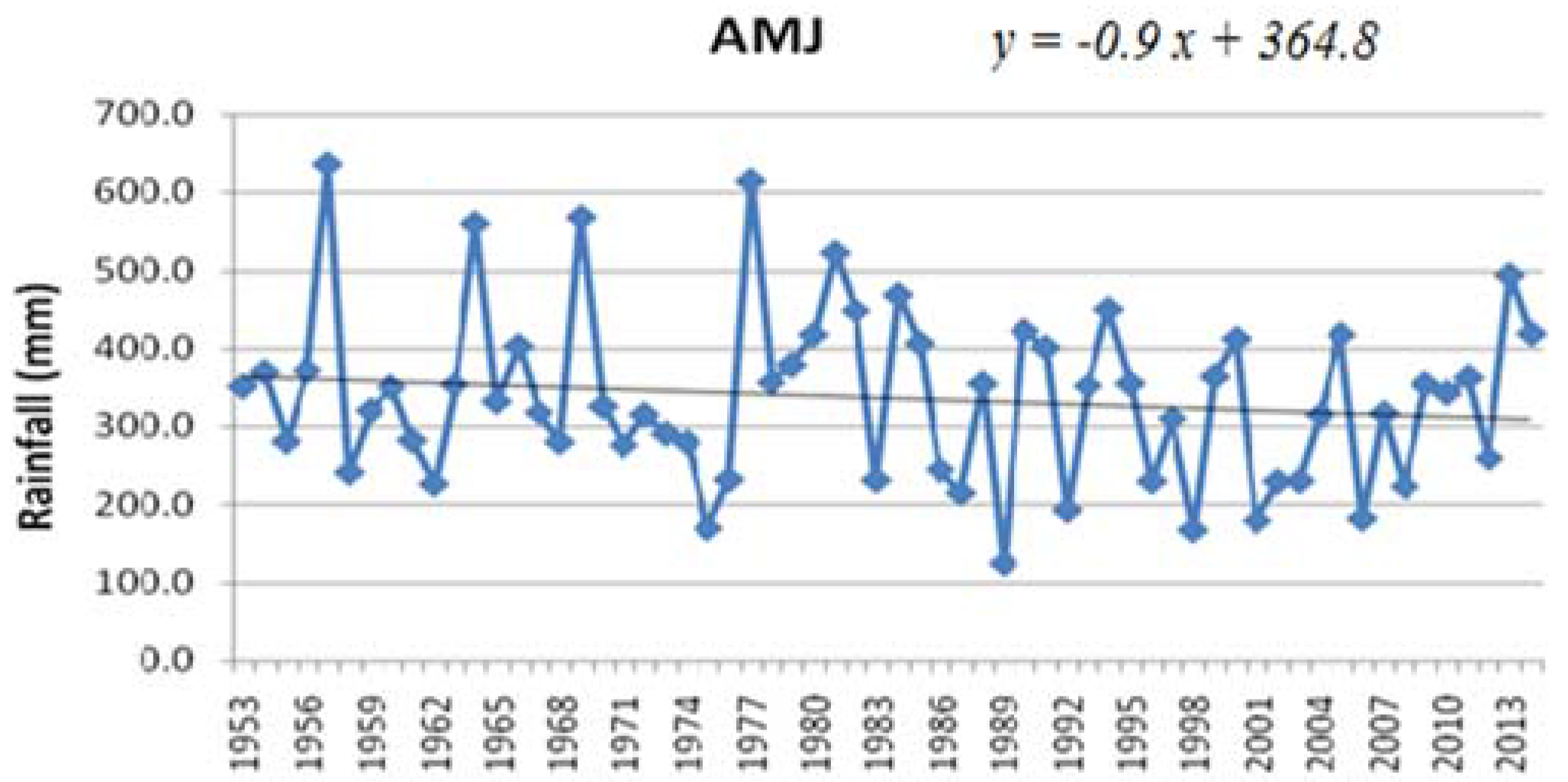
Figure 2 shows the time series of the April–June seasonal rainfall. It can be seen that there is a negative trend in the rainfall of this season. From Table 1 it is noted that although the mean rainfall has decreased, both the coefficient of variability and skewness have also decreased. This indicates a reduced frequency of extreme rainfall events during this season.
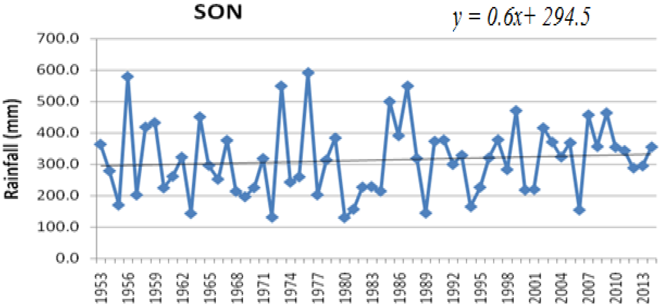
The time series of the second rainfall season; September–November (SON) is shown in Figure 3. Unlike the April–June season, the rainfall during this season has a positive trend. Just like the April-May-June(AMJ )season, both the coefficient of variability and skewness have decreased, which indicates that frequency of extreme rainfall events during this season have decreased.
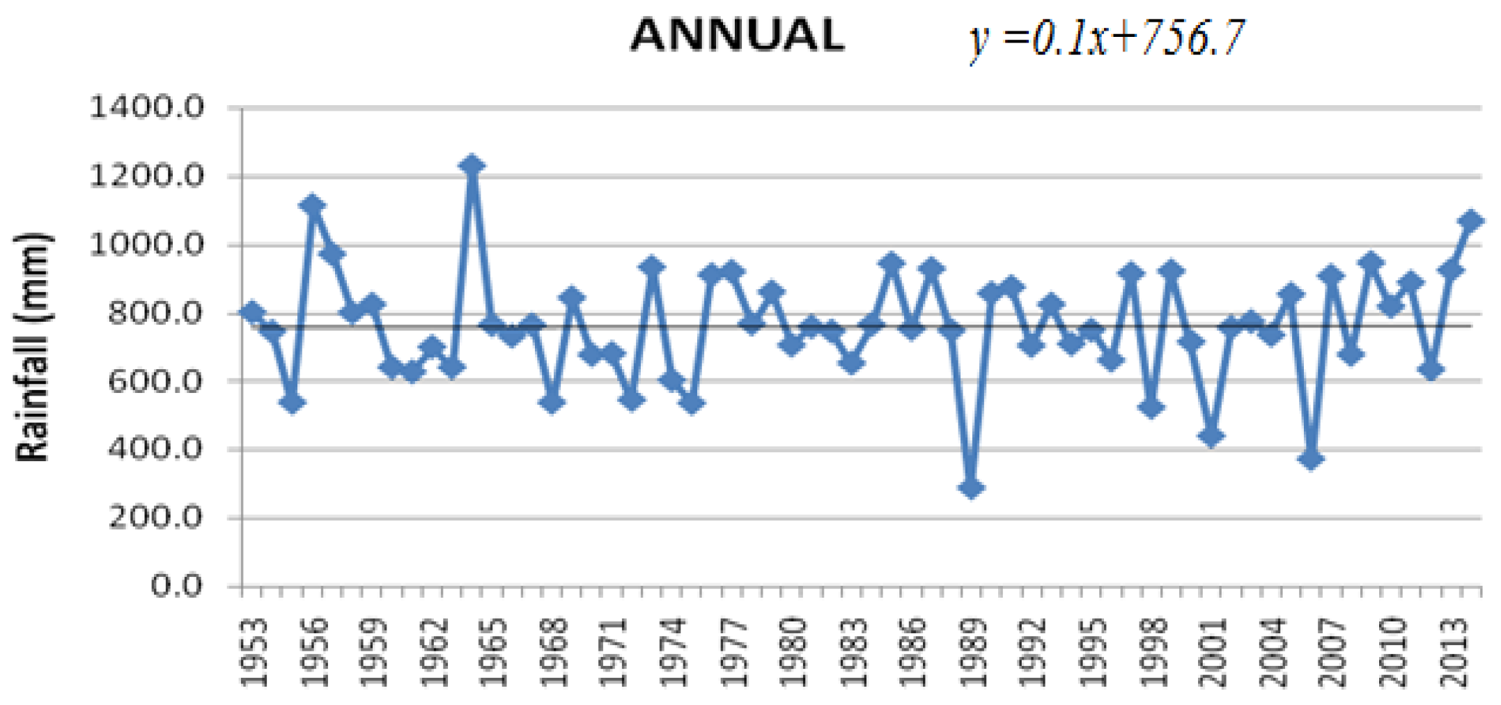
The time series of the annual rainfall is shown in Figure 4. It shows a positive trend though not significant. This may be attributed to the opposite trend of the two main rainfall seasons. Nevertheless, the annual rainfalls show increased variability and large negative skewness, as indicated by the increased frequency of annual droughts.
3.1.2. Results from Analysis of the Trends in Minimum Temperature
The time series for the March minimum temperature is shown in Figure 5. There is a positive trend indicating that minimum temperatures are increasing. From Table 2, it is seen that the skewness has decreased, and there is an indication of an increased frequency of both low and high nighttime temperatures during March.
Figure 6 shows the time series for July minimum temperatures. The series indicate a positive trend, though it is lower than March. From Table 2, it can be seen that for month the skewness has become more negative, implying that the frequency of extreme cold nights has increased.
The time of the annual minimum temperature is show in Figure 7. There is a positive trend and the skewness (see Table 2) has become positive. This means that the frequency of occurrence of higher minimum annual temperatures has increased. It can also be visually observed that the climate variables exhibit a cyclic pattern over the years from the time series graphs. However, the frequency of the cycles is on the increase over the most recent years.
3.1.3. Results from Analysis of the Trends in Maximum Temperature
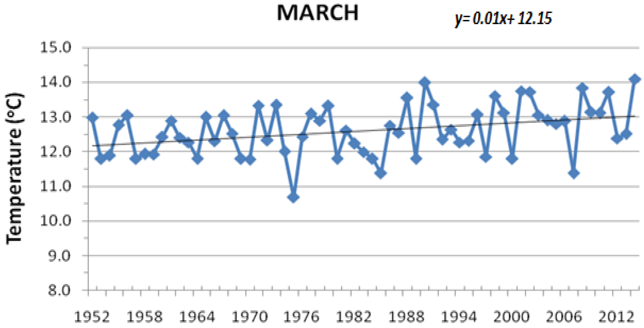
Figure 8 shows the time series of the March maximum temperature. There is a positive trend indicating rising March temperatures, which is the hottest month over the area of study. From Table 3, it can be seen that the skewness has become negative. This shows that while there has been a general increase in the temperature during this month, the frequency of occurrence of extreme low temperatures has also increased.
Figure 9 shows the time series of the May maximum temperature. The figure depicts a positive trend. As noted in the previous section, this is the coldest month over the study area. The coldest month is becoming warmer. The skewness (see Table 3) has become more positive, meaning that the frequency of episodes of extreme high temperatures during this month has increased.
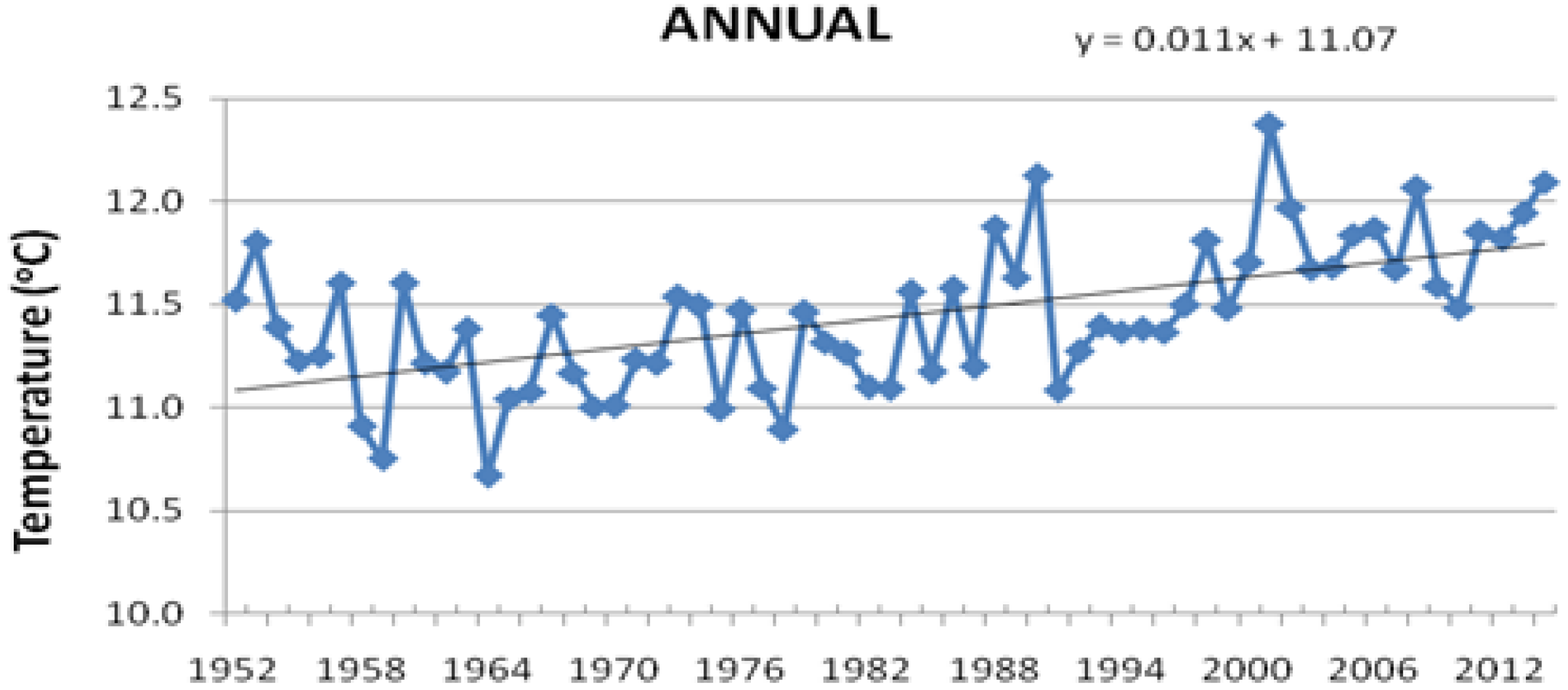
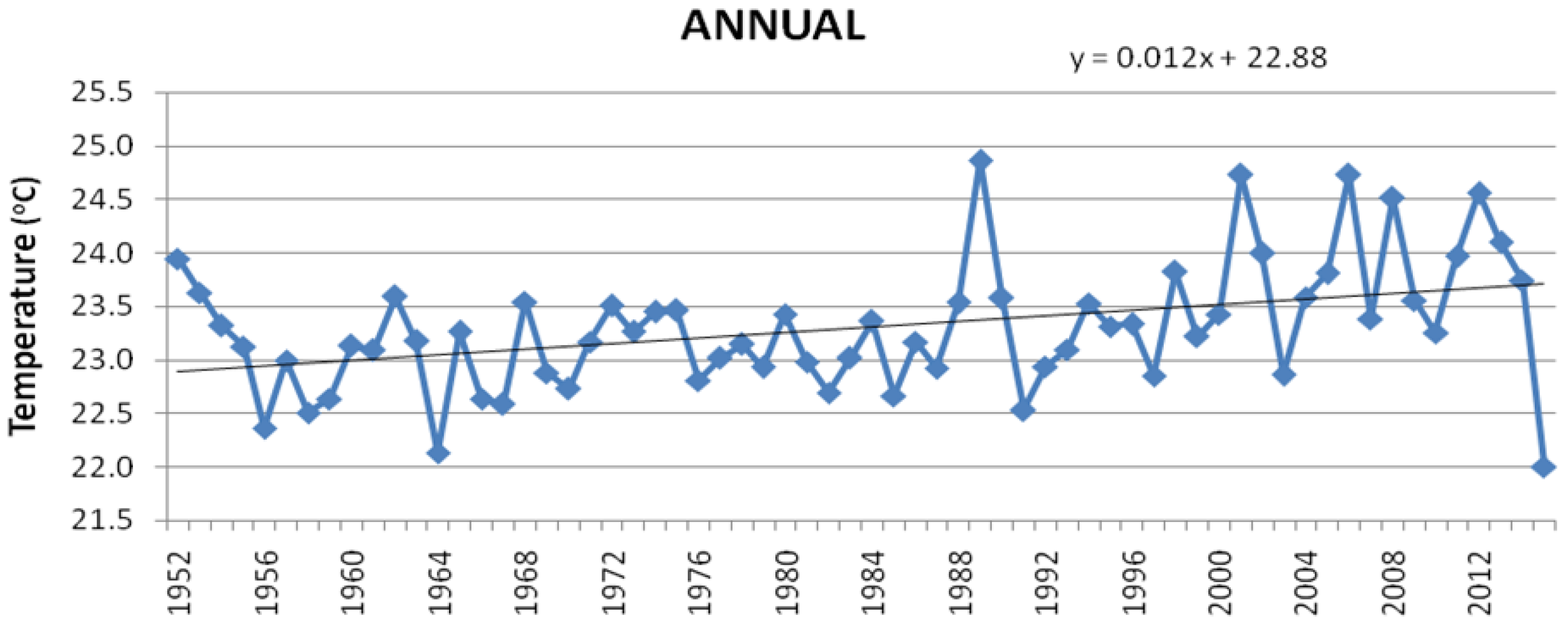
The time series of the annual maximum temperature is shown in Figure 10. There is a positive trend, and as seen in Table 3, the skewness has changed from negative to positive. This means that although previously, the frequency of extreme low temperatures on an annual basis used to be high, now the frequency of extreme high temperatures has increased. It is also observed that the coefficient of variation shows more significant fluctuations during July than other seasons. Long-term changes in annual minimum temperatures have been determined and reveal increasing trends. It can also be observed that maximum temperatures exhibited unusually high lows during March of the years 1966, 1991 and 1997, and a steady increase in May across all the years. This means May has increasingly become warmer. The annual maximum temperatures have also been rising from 1952 to the year 2012.
3.1.4. Results from Analysis of the Trends in Tea Yield
Figure 11 show the time series of the tea yield. There is a general increasing trend in the tea yield, which is an indication of improving yield over time. In the next section, the relationship between the climatic variables and tea yield is investigated.
3.1.5. Results from the Analysis Relationship between Climate Variables and Tea Yield
The results from the analysis of the relationship between the climatic variables and tea yield are discussed in this section.
3.1.6. Results from the Correlation Analysis
Correlation analysis of maximum temperature, minimum temperature and rainfall against yield are shown in Table 4. The correlation coefficient was computed between the tea yield and the monthly values of the climatic variable of the same year (concurrent) and the year before. From the table, it can be seen that the climatic variables during some months, in both the concurrent year and the previous year, were positively correlated with the tea yield. The highest correlation values were observed with the minimum temperature, while the rainfall showed the least correlation values.
In general, the correlation values were low. This prompted a further investigation into the nature of the relationship between individual climatic variables and tea yield, which is presented in the next section.
3.1.7. The Nature of the Relationship between Individual Climatic Variable and Tea Yield
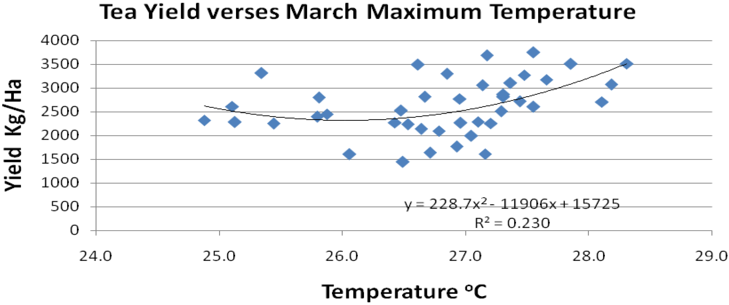
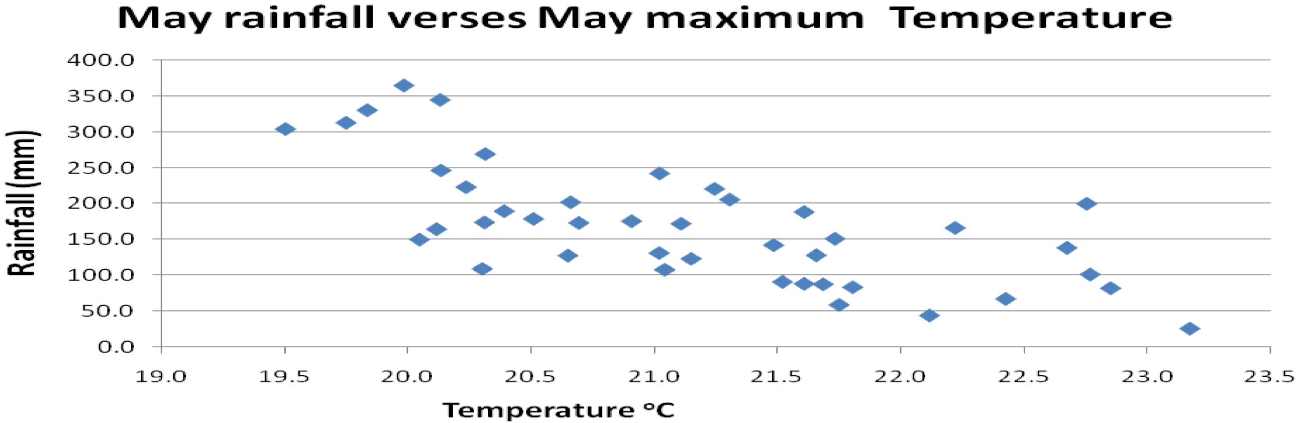
Figure 12 and Figure 13 display a scatter diagram showing the how tea yields vary with the March and May maximum temperatures, respectively. At the low end, the yield decreases with an increase in temperature, while at the upper end the yield increases with an increase in temperature. The lower end may be reflecting the fact that wet years are related with lower temperatures. On the other side, once there is rainfall, an increase in temperature should increase yield. Figure 14 shows that there is an inverse relationship between maximum temperature and rainfall. It was also noted that yield has increased over the most recent years, despite increasing climate variability over the area of study. This opens the potential for a future investigation of the possible externalities contributing to tea yield enhancement, including expanded lands for tea crop production. However, this is outside the scope of this study.
3.1.8. Results of Multiple Regression Analysis
Multiple linear models were developed to predict tea yield using climatic variables. Three model equations were developed to increase the scope for selecting the best performing model. Equation (4) was judged to be the best-fit representation of the regression model, as it explained the highest variance.
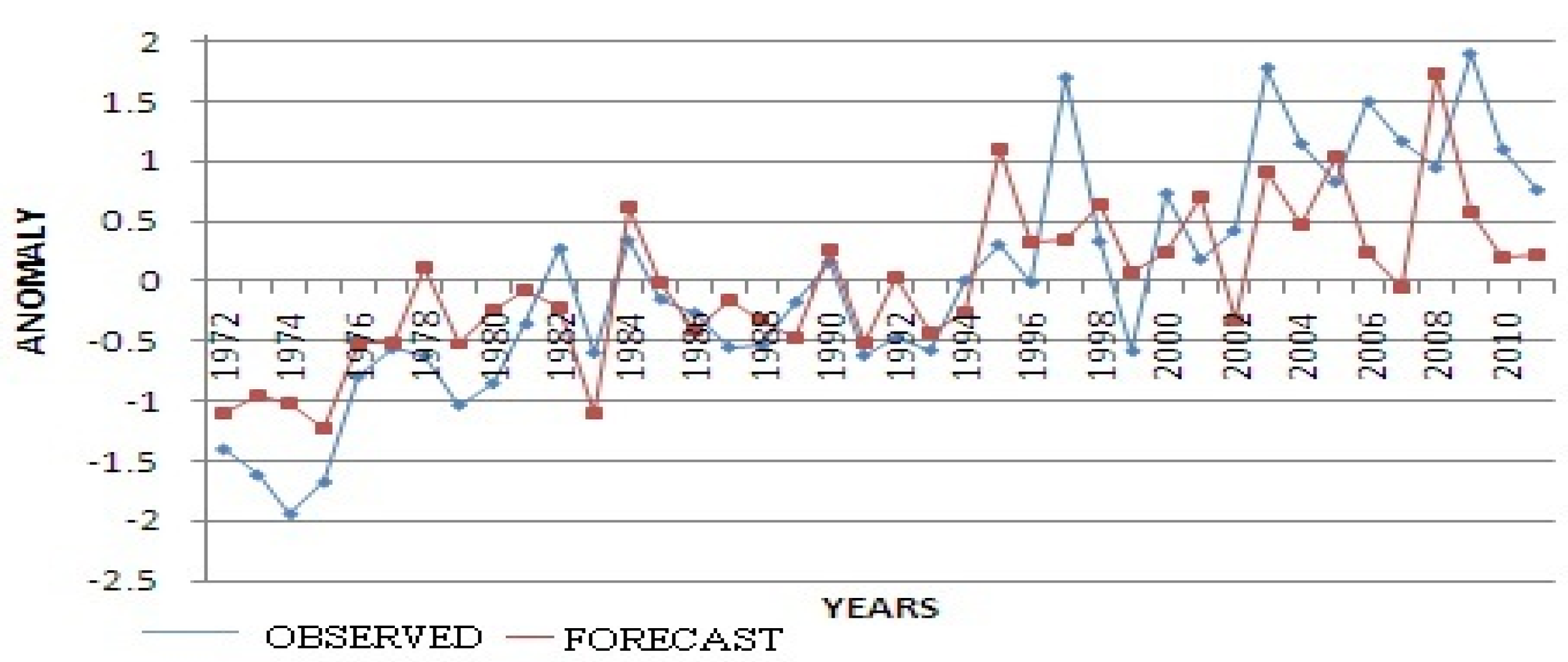
Figure 15 below shows a graph representing the regression model that was developed and judged to be best representing the best model performance.
3.1.9. Results of Model Verification
Table 5 below shows a contingency table used to verify the model. A 10-year data set between 1971 and 1981 was used to train the model. The data between 1971 and 2014 for all the variables was then used to run and test the model’s accuracy. It can be seen that 70% of model forecasts were correct. The results also show at least 50% probability of detection (POD) score, which means that at least half of the observed events were correctly forecasted. The fraction of false forecasts determined by false-alarm ratio (FAR) was observed to be low. An average post agreement rate of 77.3% was observed, indicating that the majority of the forecasts were true. For the events that were forecasted where the events occurred, the model revealed a bias of 0.5, which means the events were forecasted more than observed. However, for all events, the model revealed a bias of more than 1.0, indicating that the model over forecasted the events. An average critical success index (CSI) of 0.68 was observed. Basing on this information, the model performance was judged to be a good fit for forecasting the relationship between the variables.
4. Conclusions
Time series results of the April–June seasonal rainfall revealed a negative trend. However, a positive trend was observed during the September–November season. Extreme rainfall events reduced during these seasons. The time series of the annual rainfall showed a positive trend, though not statistically significant. This may be attributed to the opposite trend of the two main rainfall seasons. Nevertheless, the annual rainfall showed increased variability and large negative skewness, suggesting an increased frequency of annual droughts.
A positive trend was observed in the time series of March minimum temperatures, indicating that the minimum temperatures are increasing. Increased frequency of both low and high nighttime temperatures during March were also observed. A positive trend was observed in the July minimum temperatures, though it was lower than that observed in March. It was observed that the frequency of extreme cold nights has increased during March. The frequency of occurrence of higher minimum annual temperatures was observed to have increased. This shows that while there was a general increase in the temperature during this month, the frequency of occurrence of extreme low temperatures also increased. The frequency of episodes of extreme high temperatures during the month of May was also observed to have increased. Although the frequency of extreme low temperatures on an annual basis used to be high, now the frequency of extreme high temperatures has increased. There was a general increasing trend in the tea yield, which is an indication of improving yield over time. The climatic variables during some months in both the concurrent year and the previous year were positively correlated with the tea yield. The highest correlation values were observed with the minimum temperature, while the rainfall showed the least correlation values. Wet years were observed to be related to lower temperatures. Multiple linear regression models designed predicted tea yield over the area of study. However, the regressions were weak, suggesting that tea crop yields don’t respond strongly to changes in climate variables. It’s probably a very complex response, with external drivers beyond the scope of this study. Further, the possibility that there may be other variables affecting tea yield that were not investigated in this study, and probably are not climate related, can explain why the linear models had trouble reproducing the observed trends. Factors including plant breeding, genetic engineering and better tea crop management can enhance yields.
5. Recommendation
Plant yield is a very complex trait involving the interaction of many pathways and interacting factors on a molecular basis. This study made attempts to statistically link climate change signals to tea crop yields. It falls short of the genetic engineering, plant breeding, plant biomass changes, plant management and other relevant externalities that can contribute to increases in yields. Future research is therefore encouraged that can generate a statistical relationship that incorporates all the experimentally viable drivers of tea crop yields.
Acknowledgments
We thank Ininda Joseph and Fredrick Karanja for academic guidance that assisted us with academic ideas. We appreciate our Universities namely University of Nairobi, Department of Meteorology and Kibabii University, Department of Mathematics for availing a good research platform.
Author Contributions
Betty J. Sitienei was instrumental in conceptualization and methodological design. Shem G. Juma was helpful in data analysis and interpretations. Lastly, Evelyne Opere was vital in editing and formatting roles.
Conflicts of Interest
The authors declare no conflict of interest.
References
- Stocker, T.F.; Qin, D.; Plattner, G.K.; Tignor, M.; Allen, S.K.; Boschung, J.; Midgley, B.M. Climate change 2013: The Physical Science Basis; IPCC: Geneva, Switzerland, 2013. [Google Scholar]
- FCFA. Future Climate for Africa. 2016. Available online: http://www.futureclimateafrica.org/news/adapting-rwanda-growing-rwandas-tea-coffee-sectors-changing-climate/ (accessed on 19 June 2017).
- Kaison, C. Tea: World scenario. Plant. Chron. 2000, 96, 213–218. [Google Scholar]
- FAO. Available online: http://www.fao.org/fileadmin/templates/est/meetings/IGGtea21/14-4-ClimateChange.pdf (accessed on 15 July 2017).
- Lobell, D.B.; Burke, M.B. On the use of statistical models to predict crop yield responses to climate change. Agric. For. Meteorol. 2010, 150, 1443–1452. [Google Scholar] [CrossRef]
- Lobell, D.B.; Ortiz-Monasterio, J.I.; Asner, G.P.; Matson, P.A.; Naylor, R.L.; Falcon, W.P. Analysis of wheat yield and climatic trends in Mexico. Field Crops Res. 2005, 94, 250–256. [Google Scholar] [CrossRef]
- Lobell, D.B.; Bänziger, M.; Magorokosho, C.; Vivek, B. Nonlinear heat effects on African maize as evidenced by historical yield trials. Nat. Clim. Chang. 2011, 1, 42–45. [Google Scholar] [CrossRef]
- Kleijnen, J.P. Verification and validation of simulation models. Eur. J. Oper. Res. 1995, 82, 145–162. [Google Scholar] [CrossRef]
- Gordon, G.A.; LeDuc, S.K. Verification statistics for regression models. In Preprints Seventh Conference on Probability and Statistics; Atmospheric Sciences: Monterey, CA, USA, 1981; pp. 129–133. [Google Scholar]
- Ebert, E.E.; McBride, J.L. Verification of precipitation in weather systems: Determination of systematic errors. J. Hydrol. 2000, 239, 179–202. [Google Scholar] [CrossRef]
- Landau, S.; Mitchell, R.A.C.; Barnett, V.; Colls, J.J.; Craigon, J.; Payne, R.W. A parsimonious, multiple-regression model of wheat yield response to environment. Agric. For. Meteorol. 2000, 101, 151–166. [Google Scholar] [CrossRef]
- Tao, F.; Yokozawa, M.; Liu, J.; Zhang, Z. Climate–crop yield relationships at provincial scales in China and the impacts of recent climate trends. Clim. Res. 2008, 38, 83–94. [Google Scholar] [CrossRef]
- Thornton, P.K.; Jones, P.G.; Alagarswamy, G.; Andresen, J. Spatial variation of crop yield response to climate change in East Africa. Glob. Environ. Chang. 2009, 19, 54–65. [Google Scholar] [CrossRef]
- Hansen, J.W.; Indeje, M. Linking dynamic seasonal climate forecasts with crop simulation for maize yield prediction in semi-arid Kenya. Agric. For. Meteorol. 2004, 125, 143–157. [Google Scholar] [CrossRef]
- Okoth, G.K. Potential response of Tea production to climate change in Kericho County. MSc. Thesis, University of Nairobi Kenya, Nairobi, Kenya, 2011. [Google Scholar]
- Ines, A.V.; Hansen, J.W. Bias correction of daily GCM rainfall for crop simulation studies. Agric. For. Meteorol. 2006, 138, 44–53. [Google Scholar] [CrossRef]
- GOOGLE MAPS. Map of Easterhouse Churches. 2017. Available online: https://www.google.co.uk/search?newwindow=1&biw=1408&bih=648&q=easterhouse+churches&npsic=0&rflfq=1&rlha=0&tbm=lcl&sa=X&ved=0ahUKEwiJxsH-ktfLAhWKuxQKHUXYDWEQtgMIHw&gws_rd=ss (accessed on 19 June 2017).
- Araṅkacāmi, I.; Rangaswamy, R. A Text Book of Agricultural Statistics; New Age International: Delhi, India, 1995. [Google Scholar]
- Muhati, D.F. The simulated impact of deforestation on the changes in the East African climate: A GCM study. Ph.D. Thesis, University of Nairobi, Nairobi, Kenya, 2006. [Google Scholar]
- Ruxton, G.D. The unequal variance t-test is an underused alternative to Student’s t-test and the Mann–Whitney U test. Behav. Ecol. 2006, 17, 688–690. [Google Scholar] [CrossRef]
Figure 1.
Map of the area of study (Source: Edited from [17]).
Figure 1.
Map of the area of study (Source: Edited from [17]).
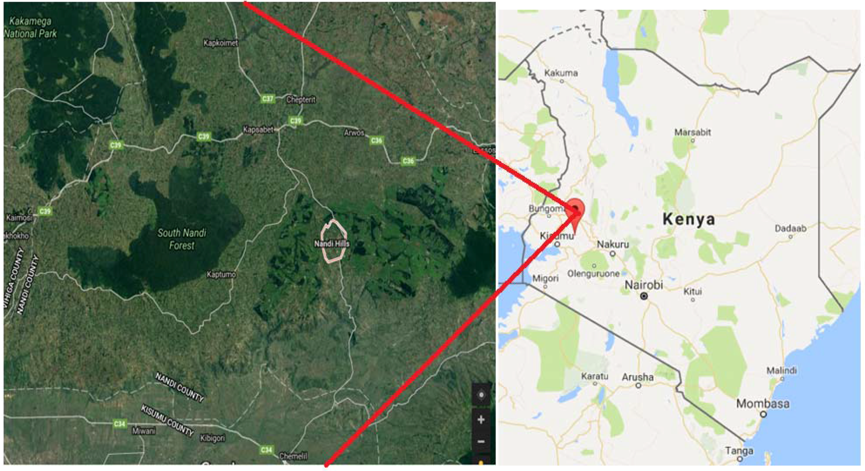
Figure 2.
The time series of the April–June seasonal rainfall.

Figure 3.
The time series of the September–November seasonal rainfall.

Figure 4.
The time series of the annual rainfall.

Figure 5.
The time series of the March minimum temperature.

Figure 6.
The time series of the July minimum temperature.
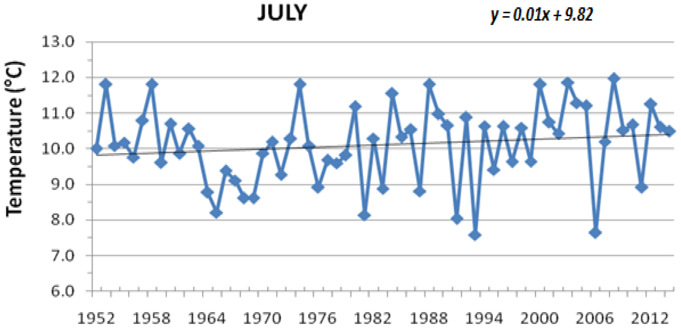
Figure 7.
The time series of the annual minimum temperature.

Figure 8.
The time series of the March maximum temperature.
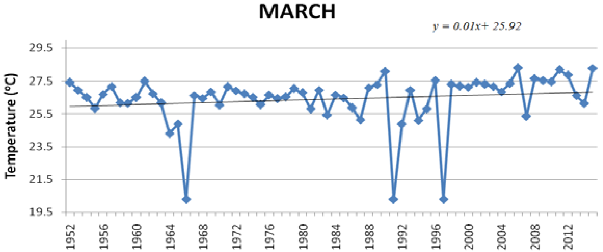
Figure 9.
The time series of the May maximum temperature.
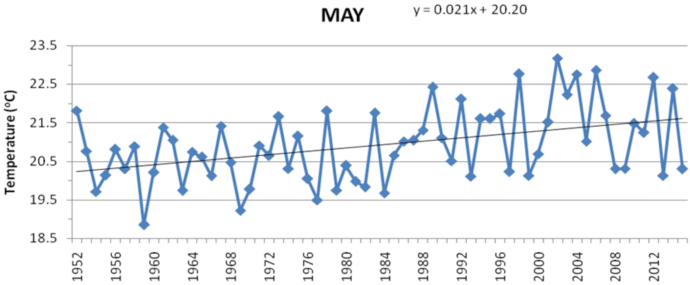
Figure 10.
The time series of the annual maximum temperature.

Figure 11.
Variation of tea yield over the area of study.
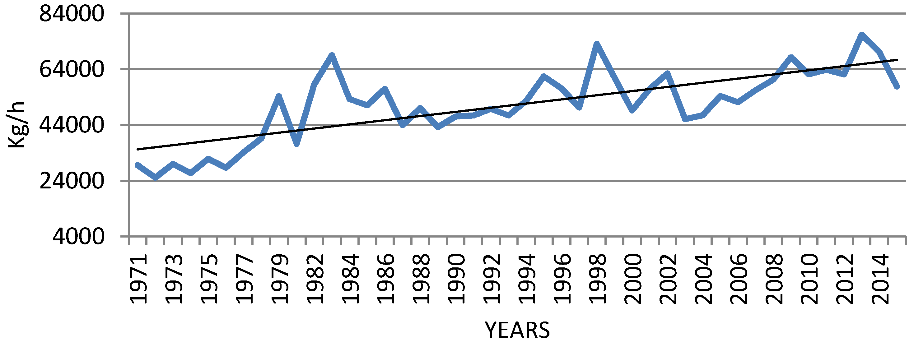
Figure 12.
The scatter diagram showing the relationship between March maximum temperatures and the tea yield.
Figure 12.
The scatter diagram showing the relationship between March maximum temperatures and the tea yield.

Figure 13.
The scatter diagram showing the relationship between May maximum temperatures and the tea yield.
Figure 13.
The scatter diagram showing the relationship between May maximum temperatures and the tea yield.
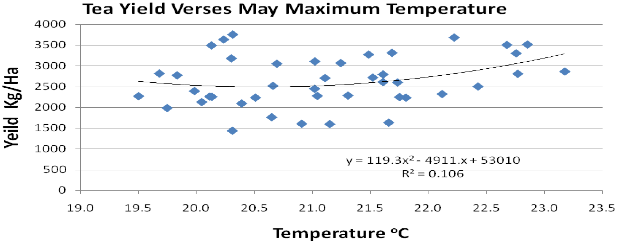
Figure 14.
The scatter diagram showing the relationship between May rainfall and maximum temperatures.
Figure 14.
The scatter diagram showing the relationship between May rainfall and maximum temperatures.

Figure 15.
Graph of regression model results for Equation (4).

Table 1.
Changes in the statistics of the rainfall (Index 1 indicates the period 1952–1983, while Index 2 is for the period 1984–2014).
Table 1.
Changes in the statistics of the rainfall (Index 1 indicates the period 1952–1983, while Index 2 is for the period 1984–2014).
| AMJ | SON | ANNUAL | |
|---|---|---|---|
| MEAN-1 | 357.70 | 294.43 | 758.21 |
| SKEWNESS-1 | 0.97 | 0.94 | 0.96 |
| MEAN-2 | 315.65 | 332.47 | 761.70 |
| SKEWNESS-2 | −0.14 | −0.03 | −1.04 |
Table 2.
Changes in the statistics of the minimum temperature (Index 1 indicates the period 1952–1983, while Index 2 is for the period 1984–2014).
Table 2.
Changes in the statistics of the minimum temperature (Index 1 indicates the period 1952–1983, while Index 2 is for the period 1984–2014).
| MARCH | JULY | ANNUAL | |
|---|---|---|---|
| MEAN-1 | 12.4 | 9.9 | 11.2 |
| SKEWNESS-1 | −0.37 | 0.30 | −0.02 |
| MEAN-2 | 12.8 | 10.4 | 11.7 |
| SKEWNESS-2 | −0.20 | −1.00 | 0.17 |
Table 3.
Changes in the statistics of the maximum temperature (Index 1 indicates the period 1952–1983, while Index 2 is for the period 1984–2015).
Table 3.
Changes in the statistics of the maximum temperature (Index 1 indicates the period 1952–1983, while Index 2 is for the period 1984–2015).
| MARCH | MAY | ANNUAL | |
|---|---|---|---|
| MEAN-1 | 26.3 | 20.5 | 23.1 |
| SKEWNESS-1 | −3.52 | 0.04 | −0.18 |
| MEAN-2 | 26.5 | 21.3 | 23.5 |
| SKEWNESS-2 | −2.40 | 0.22 | 0.21 |
Table 4.
Table of correlation between climatic variables and tea yield. (The correlation values significant at 5% significant level are bolded).
Table 4.
Table of correlation between climatic variables and tea yield. (The correlation values significant at 5% significant level are bolded).
| Month | Year Before | Concurrent Year | ||||
|---|---|---|---|---|---|---|
| Minimum Temperature | Maximum Temperature | Rainfall | Minimum Temperature | Maximum Temperature | Rainfall | |
| January | 0.258 | 0.072 | −0.110 | 0.245 | 0.114 | −0.156 |
| February | 0.281 | 0.022 | 0.070 | 0.253 | −0.020 | 0.095 |
| March | 0.401 | 0.144 | 0.164 | 0.124 | 0.077 | −0.076 |
| April | 0.232 | 0.082 | 0.030 | 0.208 | 0.236 | 0.031 |
| May | 0.344 | 0.394 | −0.011 | 0.375 | 0.270 | 0.068 |
| June | 0.242 | 0.440 | −0.148 | 0.259 | 0.295 | −0.113 |
| July | 0.130 | 0.326 | 0.309 | 0.150 | 0.245 | 0.238 |
| August | 0.224 | 0.126 | −0.042 | 0.286 | 0.039 | 0.072 |
| September | 0.347 | 0.188 | 0.160 | 0.377 | 0.078 | 0.061 |
| October | 0.298 | 0.098 | 0.055 | 0.209 | 0.242 | −0.027 |
| November | 0.156 | 0.031 | 0.113 | 0.243 | 0.195 | 0.066 |
| December | 0.145 | 0.179 | −0.010 | 0.222 | 0.157 | 0.066 |
Table 5.
Contingency table.
| Forecast | |||||||
|---|---|---|---|---|---|---|---|
| B | N | A | M-TOTALS | ||||
| B | 5 | 4 | 1 | 10 | |||
| OBSERVED | N | 0 | 6 | 4 | 10 | ||
| A | 0 | 3 | 17 | 20 | |||
| 5 | 13 | 22 | 40 | ||||
| Percent Correct | 70.0 | B | N | A | |||
| Post agreement (%) | 100 | 46.2 | 77.3 | ||||
| FAR (%) | 0 | 22.7 | |||||
| POD-HIT RATE (%) | 50 | 60 | 85 | ||||
| BIAS | 0.5 | 1.3 | 1.1 | ||||
| CSI | 0.5 | 0.35 | 0.68 | ||||
| HSS | 0.51 | ||||||
© 2017 by the authors. Licensee MDPI, Basel, Switzerland. This article is an open access article distributed under the terms and conditions of the Creative Commons Attribution (CC BY) license (http://creativecommons.org/licenses/by/4.0/).
Share and Cite
MDPI and ACS Style
Sitienei, B.J.; Juma, S.G.; Opere, E. On the Use of Regression Models to Predict Tea Crop Yield Responses to Climate Change: A Case of Nandi East, Sub-County of Nandi County, Kenya. Climate 2017, 5, 54. https://doi.org/10.3390/cli5030054
AMA Style
Sitienei BJ, Juma SG, Opere E. On the Use of Regression Models to Predict Tea Crop Yield Responses to Climate Change: A Case of Nandi East, Sub-County of Nandi County, Kenya. Climate. 2017; 5(3):54. https://doi.org/10.3390/cli5030054
Chicago/Turabian StyleSitienei, Betty J., Shem G. Juma, and Everline Opere. 2017. "On the Use of Regression Models to Predict Tea Crop Yield Responses to Climate Change: A Case of Nandi East, Sub-County of Nandi County, Kenya" Climate 5, no. 3: 54. https://doi.org/10.3390/cli5030054
Note that from the first issue of 2016, this journal uses article numbers instead of page numbers. See further details here.