Predicting Impact of Climate Change on Water Temperature and Dissolved Oxygen in Tropical Rivers


1
Department of Hydraulics and Hydrology, Faculty of Civil Engineering, University Teknologi Malaysia, 81310 Skudai, Johor, Malaysia
2
Centre for Coastal and Ocean Engineering, Research Institute for Sustainable Environment (RISE), Universiti Teknologi Malaysia, 81310 Skudai, Johor, Malaysia
*
Author to whom correspondence should be addressed.
Climate 2017, 5(3), 58; https://doi.org/10.3390/cli5030058
Submission received: 6 July 2017
/
Revised: 25 July 2017
/
Accepted: 26 July 2017
/
Published: 28 July 2017
(This article belongs to the Special Issue Climate Impacts and Resilience in the Developing World)
Abstract
:Predicting the impact of climate change and human activities on river systems is imperative for effective management of aquatic ecosystems. Unique information can be derived that is critical to the survival of aquatic species under dynamic environmental conditions. Therefore, the response of a tropical river system under climate and land-use changes from the aspects of water temperature and dissolved oxygen concentration were evaluated. Nine designed projected climate change scenarios and three future land-use scenarios were integrated into the Hydrological Simulation Program FORTRAN (HSPF) model to determine the impact of climate change and land-use on water temperature and dissolved oxygen (DO) concentration using basin-wide simulation of river system in Malaysia. The model performance coefficients showed a good correlation between simulated and observed streamflow, water temperature, and DO concentration in a monthly time step simulation. The Nash–Sutcliffe Efficiency for streamflow was 0.88 for the calibration period and 0.82 for validation period. For water temperature and DO concentration, data from three stations were calibrated and the Nash–Sutcliffe Efficiency for both water temperature and DO ranged from 0.53 to 0.70. The output of the calibrated model under climate change scenarios show that increased rainfall and air temperature do not affects DO concentration and water temperature as much as the condition of a decrease in rainfall and increase in air temperature. The regression model on changes in streamflow, DO concentration, and water temperature under the climate change scenarios illustrates that scenarios that produce high to moderate streamflow, produce small predicted change in water temperatures and DO concentrations compared with the scenarios that produced a low streamflow. It was observed that climate change slightly affects the relationship between water temperatures and DO concentrations in the tropical rivers that we include in this study. This study demonstrates the potential impact of climate and future land-use changes on tropical rivers and how they might affect the future ecological systems. Most rivers in suburban areas will be ecologically unsuitable to some aquatic species. In comparison, rivers surrounded by agricultural and forestlands are less affected by the projected climate and land-uses changes. The results from this study provide a basis in which resource management and mitigation actions can be developed.
1. Introduction
The water temperature in a river system determines the availability, activities, and type of aquatic life in the ecosystem in which it belongs [1]. Its physical properties depend on climatic variables [2], such as air temperature [3,4], and precipitation [5]. As anticipated, the potential increase of some climatic variables due to climate change is projected at both local and regional scales [6,7,8,9]. The evaluation of the impact of climate change on river water temperature and its influences on dissolved oxygen (DO) availability in some climate groups illustrates that a variation of DO concentrations, either higher or lower, can result in water quality deterioration and distortion of an aquatic ecosystem [10,11,12,13,14]. The survival of aquatic animals depends on adequate DO levels in the water body. As water temperature is inversely related to the DO concentration [15] and the fact that any change in the river water temperature alters its DO concentration, draws a unique relationship between different physical variables. In addition, other local conditions, such as land-use, pollution levels, and local hydrology increase or decrease its variability [16,17,18].
Studies have shown that tropical rivers represent one of the most diverse freshwater ecosystems in the world [19] and are also the most likely affected by anthropogenic activities and climate change [20]. Rivers in the tropics are more exposed to solar radiation with lower inter-annual and inter-seasonal climatic variation and higher water temperatures [21]. Considering all these factors, coupled with the predicted high temperatures that are manifested earlier than in other climatic groups [22], tropical rivers will be directly affected. As expected, it will impact water availability, increase climatic complexity leading to phenomena such as extreme rain events, and impairment of water bodies (such as eutrophication). Consequently, changes in species composition, distribution, and habitats will occur [23]. The impact of climate change on streams have been studied mostly in temperate systems, and there effects on a broad range of scales have been outlined, but there impact on a constant high temperatures region under dynamic climatic conditions and land-use changes little knowledge is available [21]. Because lack of adequate awareness of the implications of these physical variables might create a nonproductive aquatic ecosystem with risks to freshwater aquacultural practices and lead to economic loss [24], the need to evaluate the interaction between climate and land-use changes in tropical rivers.
In this study, the influence of climate and land-use changes and their interactions are evaluated using rivers in the Skudai Watershed as a case study. The basin is located in the southern portion of the Malaysia Peninsular. Three rivers have been selected because they represent the general characteristics of the river system in a tropical region. In order to achieve the study objective, nine different climate change scenarios were developed based on the predicted climate change in the study area. Extreme and moderate emission scenarios are integrated with three future land-use scenarios unique to each of the three rivers considered. The Hydrological Simulation Program-FORTRAN (HSPF) was used to model the hydrology, water temperature and DO concentration of the rivers using basin-wide simulation. Afterward, the model was used to project the future water temperature and DO concentration under different climates, and the different land-use scenarios initially developed. It is assumed that climate and land-use will induce an increase in water temperatures [25] and a reduction in DO concentration. These multiple stressors are expected to reduce the survival of aquatic animals in the tropical rivers in the near future [26]. The influence of climate change is likely to differ among small tropical streams depending on land-use composition in the catchment and geographical location [21].
2. Materials and Methods
2.1. Study Site
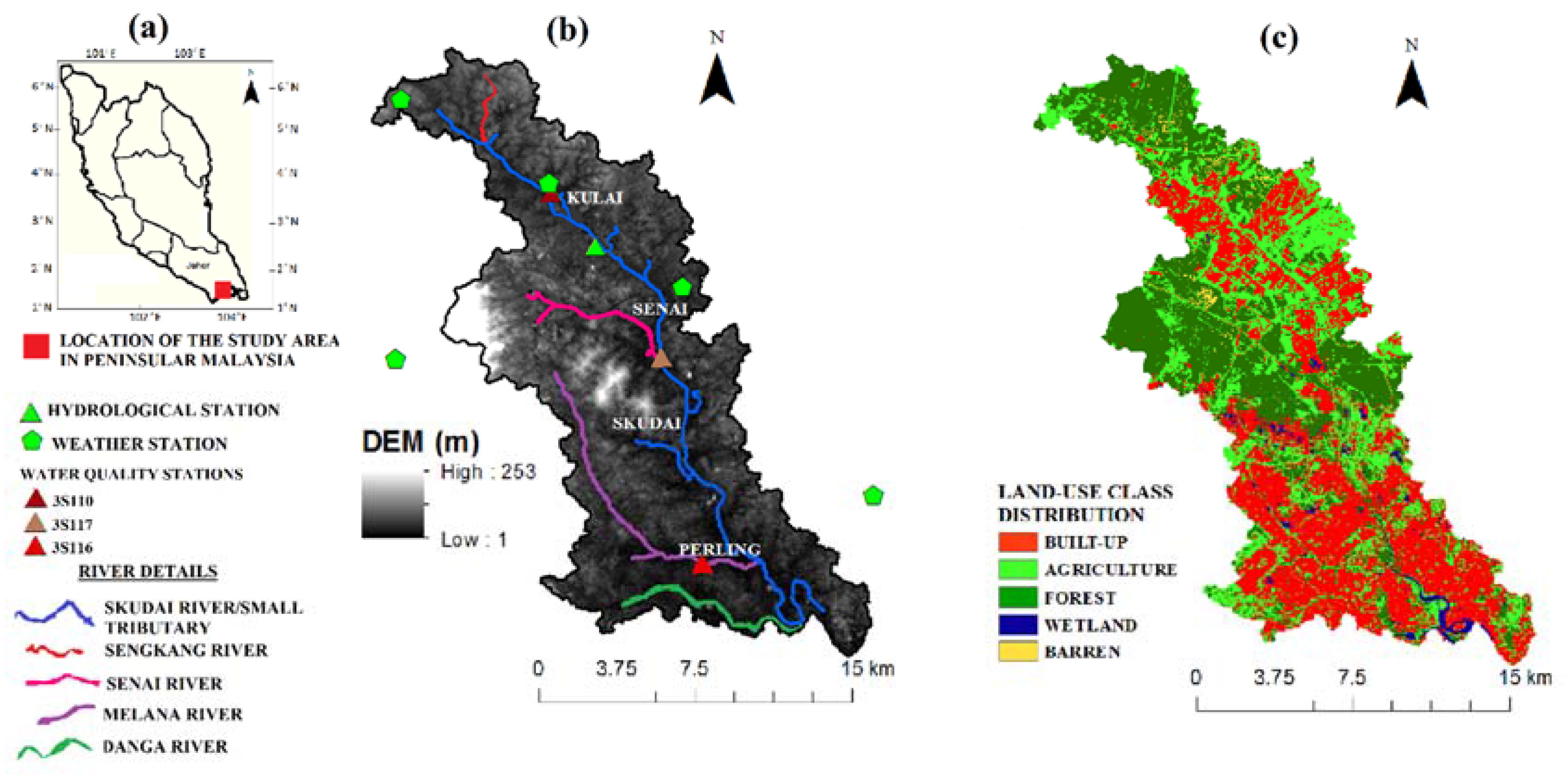
The Skudai watershed is a coastal watershed located in the southern part of the Malaysia peninsular and falls between 102°59′54.19″ E and 104°11′8.54″ E longitude and 1°56′31.67″ N and 1°22′41.16″ N latitude, as shown in Figure 1a,b. It measures 33.54 km in length by 16.29 km in width, with a total drainage area of 287.44 km2. The entire length of the main river (Skudai River) is 42.8 km and it discharges directly into the western Johor estuary.
The watershed encloses five major rivers: the Skudai River (Main River), and the Sengkang, Senai, Melana and Danga Rivers (Figure 1b). The general characteristics of the rivers are summarized in Table 1. The area is located near the equator, with a tropical climate characterised by uniformly high temperatures, high humidity and abundant rainfall [27]. It has an average annual rainfall of 2300 mm and a mean daily temperature between 21 °C and 32 °C [28]. Local soil data were collected from the soil survey division of the Ministry of Agriculture and Fisheries, Malaysia. The predominant soil texture in the watershed is sandy (78–81.2%), followed by clay (16.7–20%) and silt (2–2.1%) [29]. Based on the 2013 land-use data (Figure 1c) produced from a remote sensing technique, 36.9% of the watershed consist of urban areas, 31.5% of forestland, and 29.3% of agricultural land, while wetland and barren land cover 1.5% and 0.8%, respectively.
2.2. HSPF Model Description
The Hydrological Simulation Program-Fortran (HSPF) model is a semi-distributed model that divides the watershed into smaller sub-catchment areas which in turn are treated as a single unit [30]. It simulates hydrologic and water quality processes in streams/rivers and on both pervious and impervious land surfaces. It divides the water movement after inflows in the watershed into overland flow, interflow, and groundwater flow [31]. It uses cell-based representation of land segments and drainage channels with subdivided storage columns to present the water availability for infiltration, runoff, and groundwater recharges. HSPF typically follows a routine simulation in agreement with the three operation modules that handle all the simulation processes [32]. Basic equations for water temperature and dissolved oxygen modeling in the HSPF model were documented by Donigian and Crawford [33] and showed that the model computes the water temperature (Tw) and DO concentration on the surface, interflows and groundwater outflows from pervious and impervious land segments using the nonlinear equation defined below;
At the reaches segment, the model utilizes meteorological information to compute temperature balance. It simulates heat transfer by advection, assuming water temperature as a thermal concentration and heat are convene across the air–water interface by five heat transfer processes divided into two components [32]. The first components are those that increase heat content of water: absorption of solar radiation, absorption of long wave radiation, and conduction-convection. The components in the last segment consist of those that decrease heat content, such as emission of long wave radiation, conduction-convection, and evaporation. Each of the two steps and their mechanism is computed as separate processes combined by trapezoidal and Taylor series approximation. This method is used to determine change in water temperature due to the five heat transfer processes at a time step and is summarized by the equations;
where DO = dissolved oxygen concentration (mg/L); Tw = water temperature (°C or °F); = change in water temperature (°C or °F); Cv = conversion factor; QT = net heat exchange (kcal/m2.time); QB = net heat transport by long wave radiation; QH = heat transport from conduction-convection; QE = heat transport from evaporation; = Stephen–Boltzmann constant; Ta = air temperature (°F or °C); KATRAD = atmospheric long wave radiation coefficient; C = cloud cover (okta); = pressure correction factor depending on elevation; KCOND = conduction-convection heat transfer coefficient; w = wind speed (mi/hr. or m/s.); p = heat loss conversion factor; KEVAP = evaporation coefficient; Ps = saturation vapor pressure at water surface (mbar); and Pa = air vapor pressure above water surface (mbar). The factors KCOND, KATRAD and KEVAP are calibration parameters for water temperature modeling and have a range of values that are specified in the model input data editor [32].
While in-stream DO concentration is computed using the oxygen balance method, whereby DO and biochemical oxygen demand (BOD) state variables are maintained considering sinking of BOD, benthal oxygen demand, longitudinal advection of DO and BOD, and oxygen depletion due to decay of BOD material. The DO concentration is simulated at each time step and the saturated DO concentration is computed using Equation (1).
2.2.1. Input Data
The topographic data used in this study were obtained from the Global Data Explorer, and the pixel size is 7.5 min, one arc sec interval with 30 m resolution. They are used for watershed delineation and development of hydrological response units (HRUs). The land use components of the Skudai catchment were derived from remote sensing data. They were obtained from USGS EROS Data Centre (EDC), through the USGS Global Visualization Viewer (GLOVIS). The enhanced thematic mapping (ETM+) sensors imagery at spatial resolutions of 30 m × 30 m for the year 2013 was used to produce the land-use data.
Hourly precipitation records were collected from the Department of Irrigation and Drainage of Malaysia (DID). Other meteorological data such as dew temperature, cloud cover, solar radiation, evaporation and wind speed, and direction were obtained from the Malaysia Meteorological Department (MMD) and the National Oceanic and Atmospheric Administration (NOAA) under National Centre for Environmental Information (access on the platform of climate data online) all in hourly time step. These data were used to build an input database for model runs via the watershed data management file (WDM). Both hourly and monthly streamflow records of the watershed were obtained from the DID, and in-stream monthly water quality data were obtained from the Department of the Environment of Malaysia (DOE). Due to data limitation for streamflow, the water quality data covered only the period of the streamflow record from 2002 to 2014.
The climate change data used in this study were prepared using the dynamical downscaling method that is generated from the regional climate model known as RegCM4, derived from General Circulation Models (GCMs) based on representative concentration pathways (RCPs) scenarios. The data were produced from two emission scenarios according to the probability and location. We used the scenario RPC 4.5 and RCP 8.5, because they represent the most likely scenarios for the tropical regions for further details read [34].
2.2.2. Model Setup
The BASIN 4.1 Arc-view was used to process spatial data and coupled meteorological data via watershed data management (WDM) file. After which, the HSPF user control input file was generated and non-calibrated model of the study area was produced. The model is calibrated using observed hydrological and water quality data via parameter adjustment processes. The HSPEXP+ subprogram package [35] was used for the calibration and validation of the model. The HSPF model performance was measured by computing the coefficient of determination (R2), the Nash–Sutcliffe coefficient (NS), and percentage bias (PBIAS). The equations are listed below for the values of R2, NS and PBIAS, as suggested by Moriasi et al. [36], to evaluate the model performances, and were utilized in measuring the calibration and validation results.
2.3. Sensitivity Analysis
The model parameter sensitivity needs to be evaluated for each model application because model parameters are related to local basin physical characteristics [37]. We performed sensitivity analysis to check potential errors due to relative sensitivity of the calibration parameters and some of the model input data used in predicting water temperatures and DO concentrations from the calibration process [38]. However, due to the multiple parameter adjustments in the HSPF model calibration, a preliminary sensitivity analysis was first conducted to select the most sensitive parameters for each component section of the model (hydrological, water temperature and DO sections) that affect water temperature and DO concentration simulation results.
The significance of a single parameter to the total calibration parameters on the model that results in the deviation of the model output was evaluated using perturbation analysis [39]. We combined the range of parameter values and designed a factor perturbation that was used to adjust the parameters from their based values (as calibrated). Each parameter and input considered was adjusted by the factors of 0.3, 0.6, 0.9, 1.2, 1.5, 1.8, and 2 while allowing all other parameters to remain fixed to provide a basis for precision and comparison between each parameter [40]. The parameters evaluated by the sensitivity analysis are summarized in Table 2. The parameters were chosen based on their importance to both water temperature and DO concentration modeling. Therefore, only parameters that influenced both water temperature and DO calibration were selected for the sensitivity analysis. We used mean simulated water temperature and DO concentration values for the period 2002–2014 as the baseline to determine the variability and influence of each parameter that was considered. The mean water temperature and DO concentration were selected because of the short climatic variability that is common in the tropics [26] and to evaluate the relationship between the calibration parameters and the natural settings of the study area.
We selected three stations representing the three major land-use categories in the basin and the targeted rivers. The results were presented using graphical plots showing changes in the water temperature and DO concentration at each station due to the influence of parameters for hydrology, water temperature and DO calibration. The visual result allowed us to understand the impact of a single parameter to water temperature and DO concentration and enabled us to measure their influence on the model performance [40].
2.4. Climate Change Scenarios
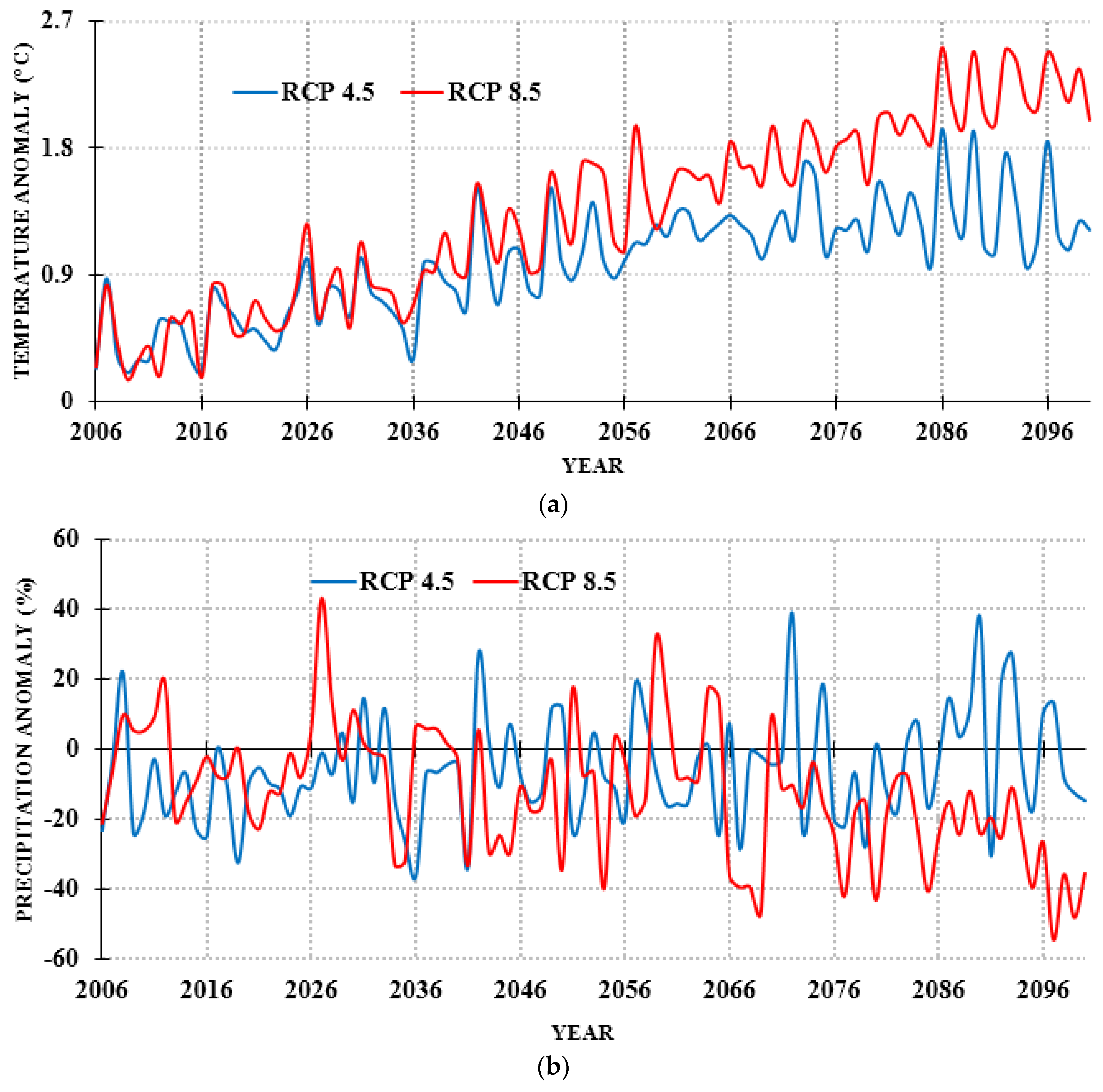
It was observed that the potential future changes in air temperature drivers were increasing independent of the General Circulation Model and emission scenario used. Hence, simulated stream temperatures are forecast to increase significantly with future climate changes [41]. In this paper, a regional climate model (RegCM4) was used to downscale the predicted daily rainfall at five rain gauge stations and the mean air temperature at the Skudai watershed. The downscaling model was first calibrated with data for the period 1956–2005. The large scale atmospheric variables were then used for the projection of local climate for the period 2006–2100 using the RCP 4.5 and RCP 8.5 emission scenarios. The rate of change in future precipitation and temperature using the baseline were produced (Figure 2a,b).
The RegCM4 model predicted an increase in air temperature from 0.1 °C to 2.6 °C (Figure 2a) before the end of the century and a percent change in rainfall from −50% to 40% (Figure 2b) in the study area considering the two RCP scenarios. The projection shows a high variability in both inter-annual and inter-seasonal rainfall. The observed anomalies based on the mean precipitation and air temperature data from 1956 to 2005 shows a percentage increase and decrease in the projected mean monthly precipitation from −50%, −30%, −20%, −10%, 0%, 10%, 20% up to 40%. The projected air temperature is to increase by 0 °C, 1 °C, 2 °C, and 2.6 °C in the future. Nine climate change scenarios were developed from the rate of change in future precipitation and temperatures using the projected precipitation and air temperature for the base years 2030 (Early century), 2050 (Mid-century), 2070 (Near the end of the century) and 2090 (End of the century), respectively, as shown in Table 3.
The observed time series data from 2000 to 2015 for air temperature and rainfall were used as a baseline for the application of the scenarios. The designed nine climate change scenarios extracted from the two projected RCP emission scenarios were inputted into the model via the Climate Assessment Tool (CAT) within BASINS program package utilizing the method described by Imhoff et al. [42].
2.5. Land-Use Scenarios
The rivers in the study area were sub-divided into two classes based on their catchment land-use. The first category was the rivers predominantly covered by forest and agricultural lands, and the second type were rivers covered by built-up areas. A developed scenario from the present land-use was designed to determine whether land-use class distribution can increase/decrease the impact of climate change on river water temperature and DO concentration in a tropical climate. Three rivers were selected for the application of land-use scenarios based on their location and proposed future development in their catchments. Table 4 shows the land-use scenarios of the three selected rivers.
The catchment of Sengkang River at present is predominantly forestland that will be converted to farmland in the future. Currently, the Senai River catchment is dominated by forest and agricultural lands but in the future agricultural land will remain unchanged and forestland will be converted to developed land. At the Melana River, it is projected that all the current forestland and agricultural land in the catchment will be converted to built-up areas with a small percent of forestland retained as a green area.
2.6. Evaluation of Scenarios
After calibration and validation of the model, the calibration parameters were maintained and used to simulate the climate and land-use scenarios earlier explained. The results obtained from the climate change scenarios were analyzed using statistical analysis. A statistical comparison method was applied to investigate the impact of each climate change scenario on the potential water temperature and DO concentration condition in tropical rivers. The method we used is referred as one-way Analysis of Variance (ANOVA) [43,44,45]. This method is a form of univariate analysis, which uses the hypothesis that the difference of one of the control variables has a significant influence on the total observed variables. In our case, we used the climate change scenarios (S1–S9) as the control variables and the daily simulated water temperature and DO concentration for each scenario as the observed variables. We considered the major river (Skudai River) for this analysis, and divided it into three segments: the upstream, mid-section and downstream. We selected Skudai River because all the other rivers in the basin are tributaries to the Skudai River as well as to observe whether the impact of climate change will vary along the river pathway (as it measures 42.8 km of length). In the case of rejecting the null hypothesis of the equality of the output of water temperature and DO concentration from the scenarios group, we used post hoc comparisons to find out how to discriminate particular water temperature and DO concentration on the basis of the scenario group. That is, we sought to determine which water temperature and DO concentration attributes from this group are best to identify the impact of climate change on tropical rivers (water temperature and DO concentration) by discriminating it from the output results of other scenarios.
The relationships between water temperature and DO concentration under climate change conditions were further evaluated. The objective was to determine the impact of climatic variables (precipitation and air temperature) on the water temperature to DO concentration relationship. Because studies have revealed the relationship between DO and water temperature to be strongly negative [46], in an effort to identify the best regression model that suited water temperature and DO concentration in the tropical climate, it was determined that the exponential model was found to be better suited to modeling low DO concentrations at higher water temperatures in temperate climate [46]. In addition, the relationship between the changes in streamflow to water temperature and DO concentration were presented using the regression model. The aim was to observe whether climate change can influence the interaction between the streamflow with water temperature and DO concentration in the tropical climate because studies suggested that stream temperatures in the moderate flow conditions were cooler than under low flow conditions [47]. Finally, the interaction between land-use and climate change was evaluated using tributary (small) rivers in the watershed (Sengkang, Senai and Melana rivers) and a graphical plot of their relationship was produced.
3. Results
3.1. Basin-Wide Simulation Result of HSPF Model
3.1.1. Hydrological Simulation
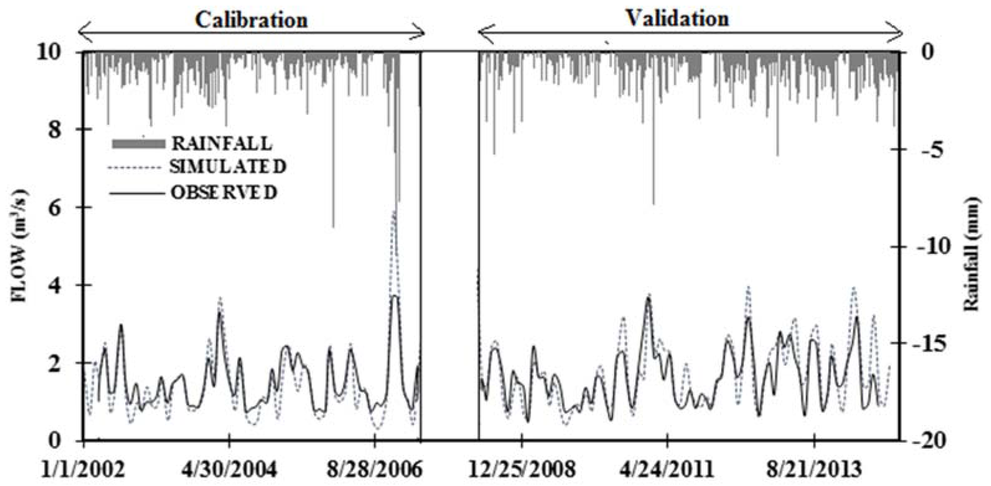
The gauge station for streamflow and water quality were in different locations (Figure 1b); therefore the hydrological modeling (calibration of streamflow) result was separated from the water temperature and DO concentration models. Initially, the HSPF model was calibrated using monthly observed streamflow data. Sensitivity analysis of the calibration parameters was evaluated against simulated flow time series generated at the hydrological gauge station of the Skudai watershed using flow time series from January 2002 to December 2014. Five parameters were more sensitive out of the thirteen parameters adjusted during the calibration processes (listed according to their sensitivity index from higher to lower): Lower zone nominal soil moisture storage (LZSN), Index to infiltration capacity (INFILT), Lower zone evapotranspiration (ET) parameter (LZETP), Base groundwater recession (AGWRC), and Upper zone nominal soil moisture storage (UZSN) parameter. Sequel to the calibration and validation of the model, a statistical performance check confirms a proper calibration and validation of the model as shown in Table 5 [36].
The coefficient of determination (R2) shows that the model describes 89% of the total variability in the observed data onto monthly flow level. The model performance was good at 11% overestimation of flow for a 53 months simulation period, and the validation result shows a satisfactory performance with captured variability of 83% and an overestimation of 17% (Figure 3).
3.1.2. Water Temperature and Dissolved Oxygen Simulation
Modeled stream temperatures and DO concentrations were compared to the observed monthly data for water temperatures and DO concentrations for the period from 2002 to 2014 periods at three monitoring locations (Figure 1b). The three locations were selected out of nine monitoring locations in the Skudai watershed because they captured the water temperature and DO concentration level of the three targeted rivers used as a case study in this research. The coefficient of the determinant (R2) between predicted and observed monthly water temperature ranged from 0.64 (station 3S117—the intersection between the Senai and Skudai Rivers) to 0.74 (3S110 station 3S110—downstream of Sengkang River). Conversely, the R2 values for the DO concentration ranged from 0.55 to 0.65. The results of statistical tests performed between observed and simulated monthly water temperature and DO concentration are presented in Table 6.
The average (mean) monthly and standard deviation values indicated that the model produced more variability in estimated DO concentration values, and less variability in the simulated water temperature values when compared with the observed values. However, the paired sample t-test indicated that the differences between the means of measured and simulated monthly water temperature and DO concentration were not significant at the 95% confidence level, except for the result of the simulated DO at station 3S117. However, the R2 and NSE values showed a better relationship between simulated water temperatures and DO concentrations with the observed values. Figure 4a–c compares graphically the observed and the simulated monthly water temperature and DO concentration values for the modeled period.
3.2. Sensitivity Analysis
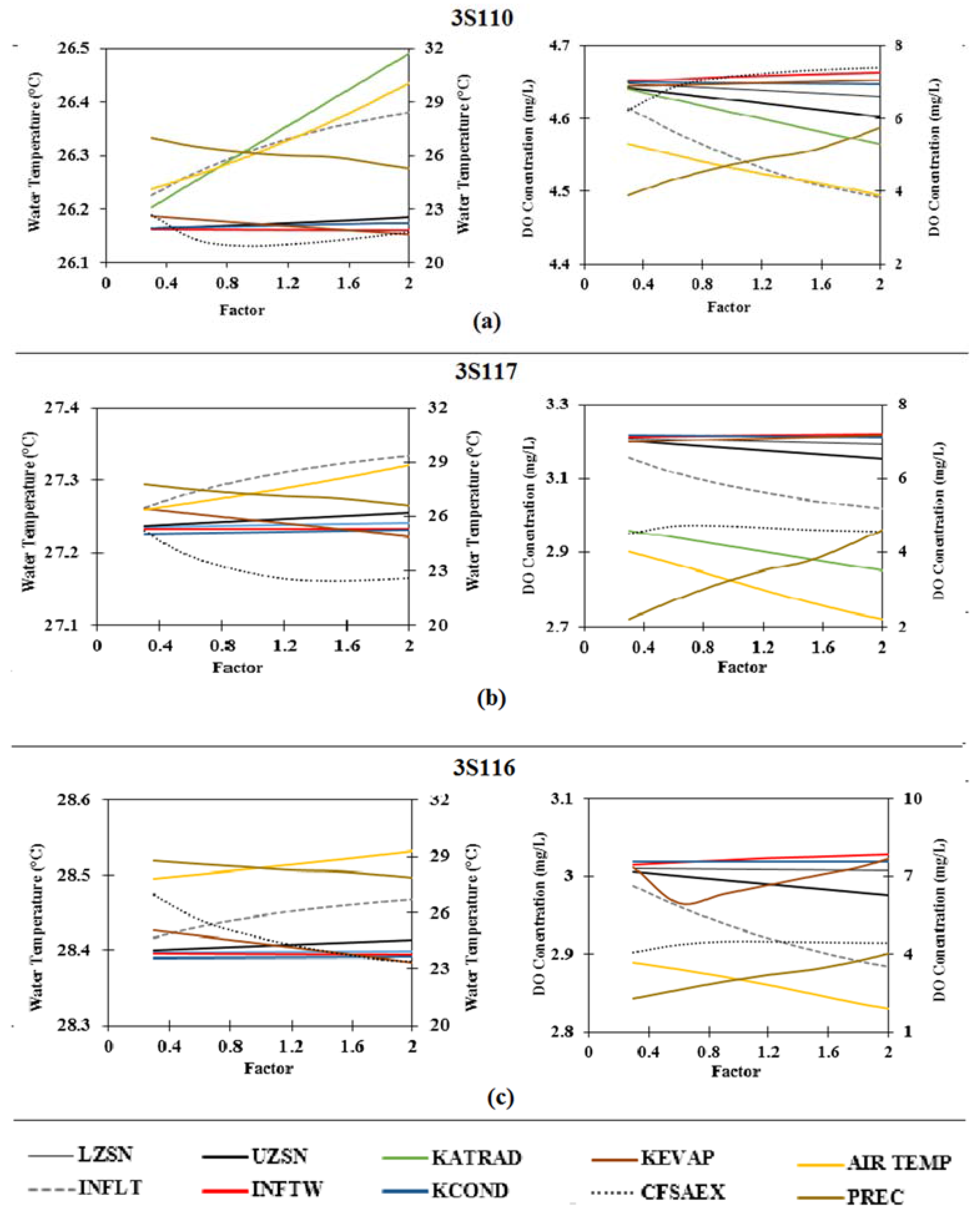
The sensitivity analysis results from the process designed to identify the most sensitive parameters selected from the preliminary sensitivity analysis of 13 parameters under hydrological calibration processes indicate that Index to Infiltration Capacity (INFILT) was the most important hydrological calibration parameter in our simulation (Figure 5), with Upper Zone Nominal Soil Moisture storage (UZSN) and Interflow Inflow parameter (INFTW) following in relative importance. The lower zone nominal soil moisture storage (LZSN) parameter was the least sensitivity among them. The nonlinear response shown by the INFILT parameter aligned with the core equations of the model [32]. However, UZSN, INFTW, and LZSN showed a linear response in this analysis. On the other hand, when INFILT was increased up to a unit, the water temperature increases by 0.04 °C/unit (per unit means, at every increase of 0.3 of the calibration parameter values) to 0.01 °C/unit and the DO concentration decreases by 0.03 mg/L/unit to 0.01 mg/L/unit. In addition, as the UZSN, LZSN and INTFW parameters were increased up to a unit, the water temperature increases from 0.003 °C/unit to 0.0002 °C/unit and DO concentration decreases by 0.003 mg/L/unit to 0.0002 mg/L/unit at all three stations.
For the other parameters, the correction unit for solar radiation (CFSEAX) parameter showed the highest sensitivity, followed by long wave radiation coefficient (KETRAD), then evaporation coefficient (KVAP), and the least was conduction-convection heat transport coefficient (KCOND) parameter. On increasing the initial CFSEAX parameter value above its base value to a unit, the water temperature increased by 1.4 °C to 0.2 °C per unit, whereas DO concentration decreased by 0.6 mg/L/unit to 0.02 mg/L/unit. The second important parameter was KETRAD when increased up by a unit; it resulted in an increased in the water temperature by 0.04 °C/unit to 0.01 °C/unit and DO concentration decreased by 0.02 mg/L/unit to 0.008 mg/L/unit in all the three stations considered. KCOND and KVAP parameters when increased up to unit, produced an increased in water temperature by 0.002 °C/unit to 0.0003 °C/unit and DO concentration decreased by 0.01 mg/L/unit to 0.0008 mg/L/unit across the three stations.
We also considered the sensitivity of the important input data that were critical to this research and significant to the model output on water temperature and DO concentration simulation. Two input data were analyzed, the air temperature and precipitation. Air temperature showed higher sensitivity than precipitation to both water temperature and DO concentration, and precipitation displayed a nonlinear response to water temperature with sensitivity fluctuating from 0.5 °C/unit to 0.1 °C/unit. The same response was observed with DO concentration with sensitivity varying from 0.5 mg/L/unit to 0.2 mg/L/unit. While the precipitation indicates a nonlinear response to water temperature and DO concentration, the air temperature showed a linear response. The sensitivity of the air temperature to water temperature fluctuates between 1.2 °C/unit to 0.2 °C/unit and DO concentration sensitivity values varied from 0.3 mg/L/unit to 0.1 mg/L/unit.
By the sensitivity analysis performed, it was concluded that the water temperature and DO concentration was highly sensitive to CFSEAX, air temperature, precipitation and then the INFILT parameter. The CFSEAX parameter determined the percent of the river surface that was exposed to direct solar radiation. These results were supported by the findings of Leach et al. [48], i.e., the density of the vegetation along the rivers determines the water temperature level. High infiltration reduced the quantity of the runoff, resulting in a low flow condition and increases the exposure time of the water to both air temperature and solar radiation. However, increased precipitation caused more water to flow out as runoff and therefore resulted in lower water temperature and increased DO concentration. Increased air temperature will promote increased water temperature with decreases in DO concentration, as conduction-convection has variable effects on water temperature due to increasing solar radiation [48,49].
The results of the sensitivity analysis show that the uncertainty in the model parameters has no effect on the simulation results of some of the model outputs considered (those parameters with low sensitivity). However, the consideration of the uncertainty in the model parameters that show high variability in the model output indicates their tendency to influence the simulation result. The two highly sensitive parameters discussed earlier (INFILT and CFSEAX) control the uncertainty in the water temperature and DO concentration simulated by the model. In addition, these parameters can improve the performance of the model, as they have a short range of parameter adjustment (see Table 2) as compared to the other parameters with low sensitivity. Therefore, they can be considered for the reduction of the uncertainty in the model output.
Furthermore, the sensitivity results of the weather data (air temperature and precipitation) show that accurate measurement of weather data is essential for the model simulation. In our case, the integration of the data from the five rain gauge stations in the model improved the accuracy of the precipitation data as it captured the rainfall distribution in the Skudai watershed. For air temperature, only one station was used as a data source because it was the only available location in the study area. However, it will not affect the model output considerably because weather data are fixed to their measured values (or nominal values) without any uncertainty [50].
The vertical axis was divided into two components (Figure 5). The left hand side (LHS) axis represents the parameters/input variables with small variability for the water temperature and DO concentrations (LZSN, UZSN, KATRAD, KEVAP, INFILT, INFTW, and KCOND). The right hand side (RHS) axis represents the parameters/input variables with wide variability for water temperature and DO concentration (AIR TEMP, PREC, and CFSAEX).
3.3. Climate Change Assessment
A tropical climate is associated with consistently high temperatures and abundant rainfall. Equally, future climate projections show further increases in air temperature and more variable rainfall. The integration of the projected climate change using nine climate scenarios into the calibrated model of a tropical catchment provides information on the possible shifts in the river water temperature and DO concentration in the future. In this subsection, we present the results of the analyses of the feature group scenarios, as explained in Section 2.6.
3.3.1. Analysis of the Water Temperature Variability under Climate Change Scenarios
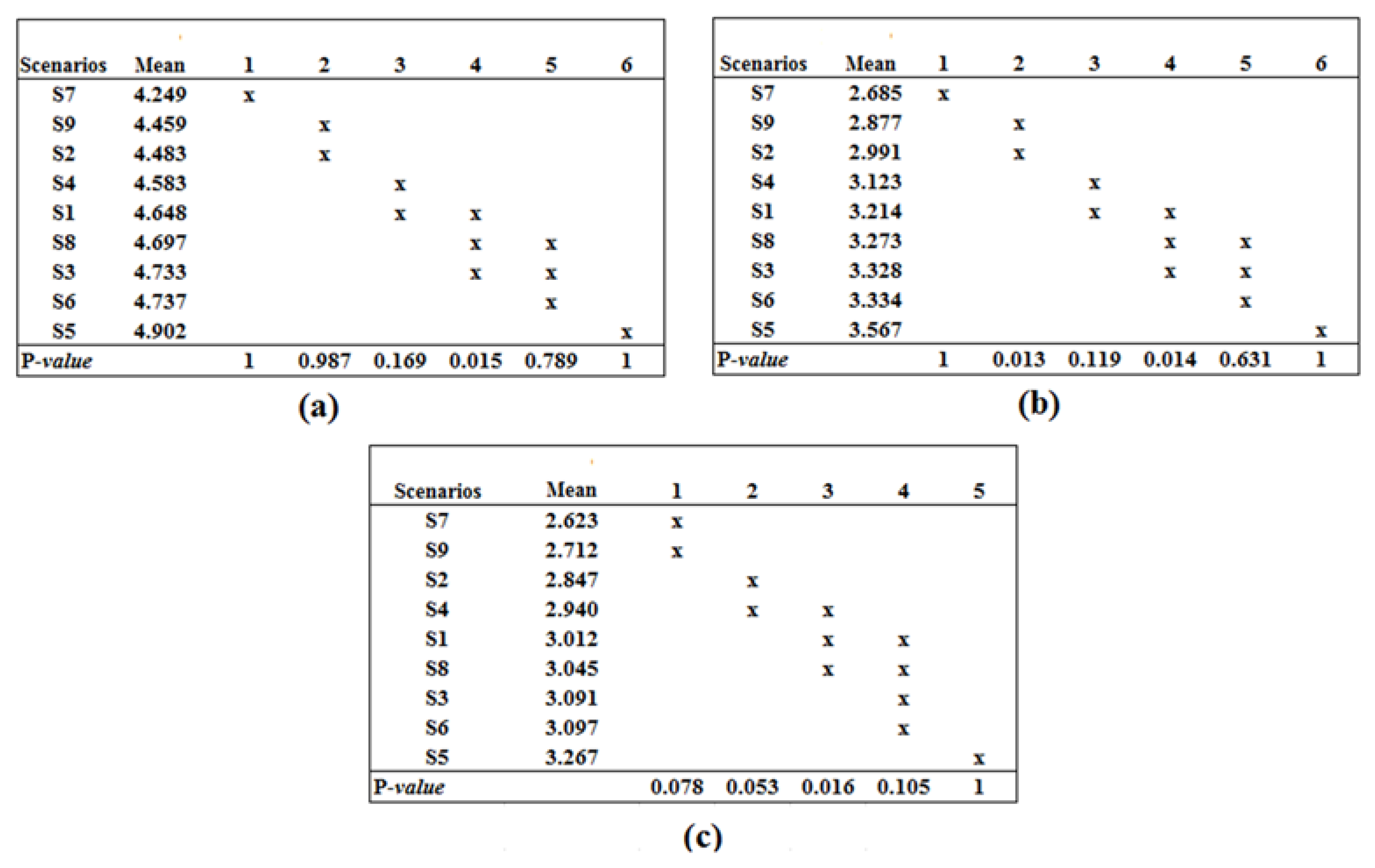
The results of the ANOVA analysis showed that the mean values of the analyzed water temperatures along the river pathway (upstream, mid-section and downstream) significantly differed among the scenarios (p < 0.01) as shown Table 7. From the univariate results (ANOVA), we conclude that the water temperature varied significantly for each scenario because the F-distribution of the nine scenarios produced p-value less than 0.01. These results allowed us to apply post-hoc comparisons for each of the simulated water temperature outputs from the nine climate scenarios. The results are presented in the form of tables made up of homogenous subsets of scenarios as shown in Figure 6. The results of the post hoc analysis revealed that all sections of the river pathway considered separately influence each scenario to a large extent. However, we used p-values for each subset to define the significant scenarios, because the p-value indicates that the scenario subset produced the same water temperature at each section of the river (p > 0.01). Scenarios S7 and S9 are well distinguished from the other scenarios in the upstream portion of the river. Scenario S7 has a mean water temperature higher than that of S9 scenario, with the fact that S9 scenario has a higher air temperature compared to S7. The result indicates that the upstream water temperature of the river is more sensitive to precipitation changes than to air temperature. It was further buttressed by the subset Group 1 scenarios, showing that scenarios S1, S3, S5, and S6 are similar. Thus, it is difficult to differentiate these scenarios based on water temperature conditions, as they have no statistically significant differences. These group scenarios have a common feature of positive precipitation. In addition, no single scenario is well distinguished from the other scenarios for the mid-section and downstream portions of the river, meaning that, from the mid-section of the river to the downstream section, the water temperature output produced by all the scenarios cannot be distinguished by single significant statistical difference but only in a group and at subset level.
However, the result indicates that in the mid-section and downstream section a decrease of precipitation above 24% (scenario S9) cannot be distinguished by mean air temperature output (i.e., no significant difference). In addition, an increase in precipitation from 0% (S1 scenario) to 9% (S8 scenario) produced similar mean water temperatures independent of the air temperature increase (from 0 °C to 2 °C).
In general, the variability of water temperature under climate changes conditions decreases from upstream to downstream. It can be observed from the mean differences of water temperature along the three section of the main river (Figure 6). In addition, the water temperature along the river pathway increases at the minimum of 1 °C between each section of the river. The Homogenous subset group classified all the scenarios based on the outcome of the water temperature conditions. For example, subgroup one scenarios produced a lower impact on water temperature compared to subgroup three scenarios and subgroup five scenarios. Therefore, scenarios S7 is the best scenario to identify the impact of climate change on tropical rivers follow by scenario S9, but the least scenario that poorly identified the impact of climate change on water temperature in a tropical river is scenario S5 and S6.
3.3.2. Analysis of the DO Concentration under Climate Change Scenarios
The results of the one-way ANOVA illustrate that the mean values of the DO concentrations were significantly different for the group scenarios (p < 0.01). Table 8 shows the results of the analysis in detail. The homogeneous grouping indicates (Figure 7) that, at the upstream, S7 and S5 scenarios produced a different mean DO concentration at subset levels one and six, respectively. However, the rest of the scenarios provided mean DO levels with no statistical significant difference at various subset levels. The same condition was observed at the mid-section of the Skudai River, while at the downstream only scenario S5 produced a distinctive mean DO concentration. When a mean value for a particular scenario is distant from the other mean values, then this scenario is very easy to distinguish from the others.
For example, scenarios S7 and S5 are well distinguished from the other scenarios on the upstream and mid-section portion of the river (Figure 7), whereas mean values of the downstream for scenario S1, S3 and S8 are similar, and these scenarios are situated in the same group, so these scenarios are difficult to differentiate based on mean DO concentration values. Similarly, at the upstream and mid-section portion, scenarios S3, S6, and S8 are in the same group and possess no statistically significant difference. However, scenario S5 is distinguished among the scenarios in all the three sections of the river.
The results show that the DO concentration in the river follows a uniform pattern as indicated in the group classes. The DO concentration homogenous scenario levels differ from those for the water temperature. For the DO concentration, S5 scenario is the best scenario to identify the impact of climate change on tropical rivers followed by scenario S6, but the scenarios that most poorly identified the impact of climate change on water temperature in a tropical river are scenarios S7 and S9. The results show that the mean DO concentration produced by each scenario considering the three section of the river, it shows that the mean DO at the upstream is higher compared with the mid-section and downstream portions of the river. The last two sections of the river produced related DO concentrations across the nine scenarios.
Comparing the outcome of the post-hoc comparisons for water temperature and DO concentration, the result shows that the two constituents have a negative correlation. However, the relationship between these two parameters will be discussed in the next section.
3.3.3. Interaction between DO Concentration and Water Temperature under Climate Change Scenarios
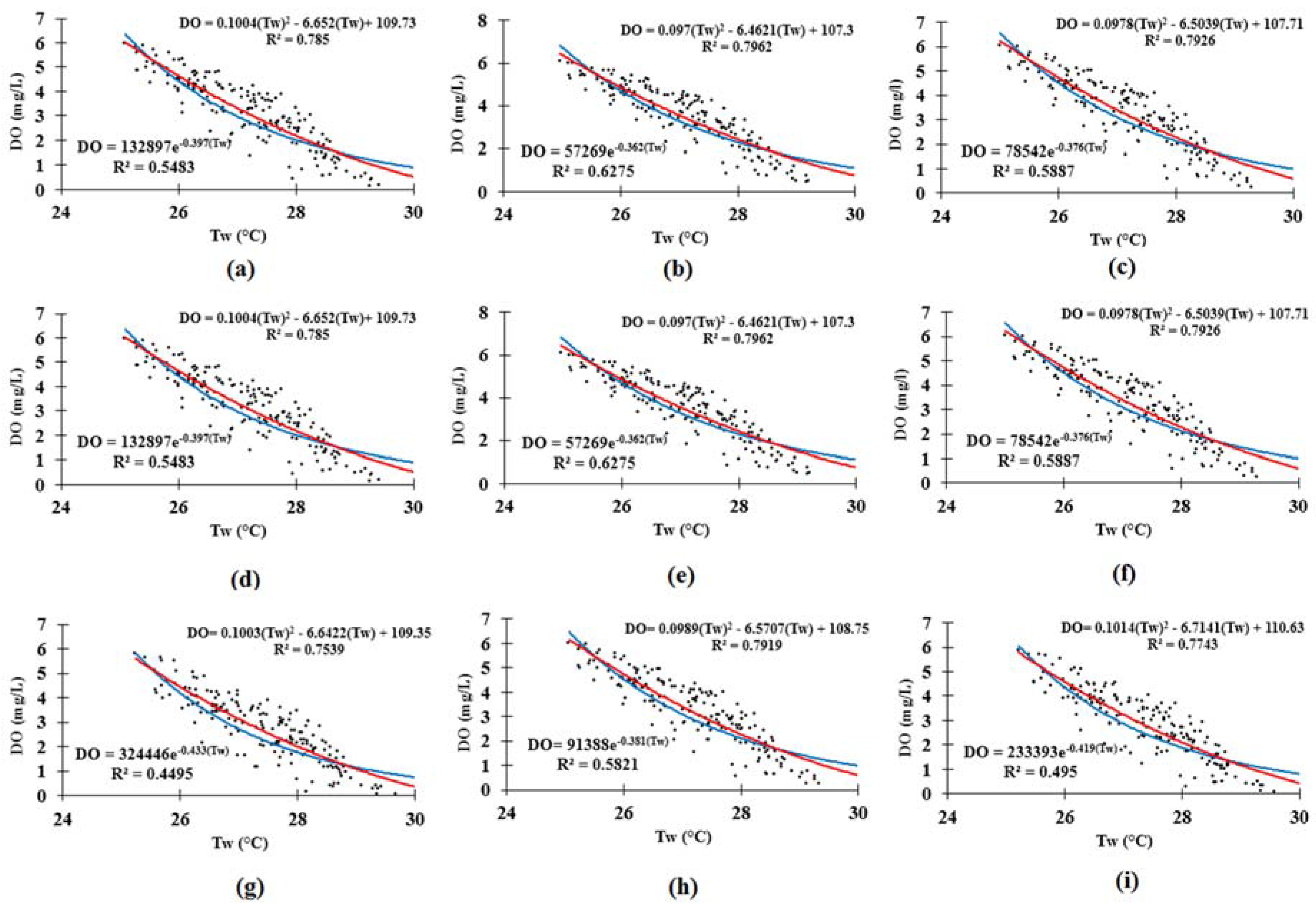
Figure 8 presents the set of regression models that were developed based on a change in water temperature and DO concentration under climate change conditions with monthly time steps. Regression models for the mean DO concentration and water temperature proved to be a poor fit when using an exponential regression model compared to the polynomial model because the coefficient of the determinant (R2) for the exponential regression is lower than that of the polynomial regression. From the regression results (Figure 8), the relationship between DO and water temperature is stronger under the increased precipitation scenarios in comparison to then decreased precipitation scenarios. Scenarios S7 and S9 produced R2 values of 0.449 and 0.495 using the exponential regression model and 0.754 and 0.774 values for polynomial regression model, respectively, while scenarios S3, S5, S6, and S8 produced R2 values of 0.588, 0.628, 0.589 and 0.582 derived from the exponential regression model and 0.793, 0.796, 0.793 and 0.792 derived from the polynomial regression model, respectively. This result shows that climate change conditions will not affect the relationship between DO and water temperature significantly. On the other hand, the variations in the regression models indicate the impact of climate changes on the water temperature and DO relationship. It also shows that the scenarios produced a similar but different result at each precipitation and air temperature fluctuation. Finally, low DO and high water temperature are best related using the polynomial regression model compared with the exponential regression model in the studied rivers. However, river flow conditions might influence this relationship because the changes in timing and form of precipitation can affect the timing of maximum and minimum flows in a river system [51].
3.3.4. Interaction between Streamflow, Water Temperature, and DO Concentration under Climate Change Conditions
The correlation between streamflow alongside river water temperature and DO concentration for each scenario is presented in Figure 9. The results indicate that the relationship between streamflow and DO are better than that between streamflow and water temperature. However, the variability in streamflow shows slightly more impact on water temperature than DO concentration. It can be observed from the R2 values across the nine scenarios.
The regression model indicates the impact of climate change on the water temperature and DO conditions because each scenario produces a different maximum flow condition with a different average flow. For example, scenario S5 produced a maximum streamflow of 24 m3/s and an average flow of 8.5 m3/s, while scenario S7 produced a maximum streamflow of 10 m3/s and an average flow of 4.9 m3/s. As these scenarios produced different streamflow condition, so they influenced the DO and water temperature levels. For example, scenario S5 produced the maximum water temperature value of 30.5 °C with DO level of 0.57 mg/L at a flow of 1.0 m3/s, but scenario S7 generated a maximum water temperature of 30.8 °C with DO level of 0.20 mg/L at a flow of 1.0 m3/s. In summary, the regression model indicates that climate change scenarios have a tendency to modify the streamflow pattern in the tropical rivers and subsequently influence the water temperature and DO concentration. However, the variations in the streamflow do not indicate a severe impact on the water temperature compared to the DO concentration. The evaluation of the impact of climate change on water temperature and DO level under streamflow variability discussed in this section and compared with the previous analysis indicates they would have a small prospect across the nine scenarios.
3.4. Influence of Land-Use on Water Temperature and DO Concentration under Climate Change Scenarios
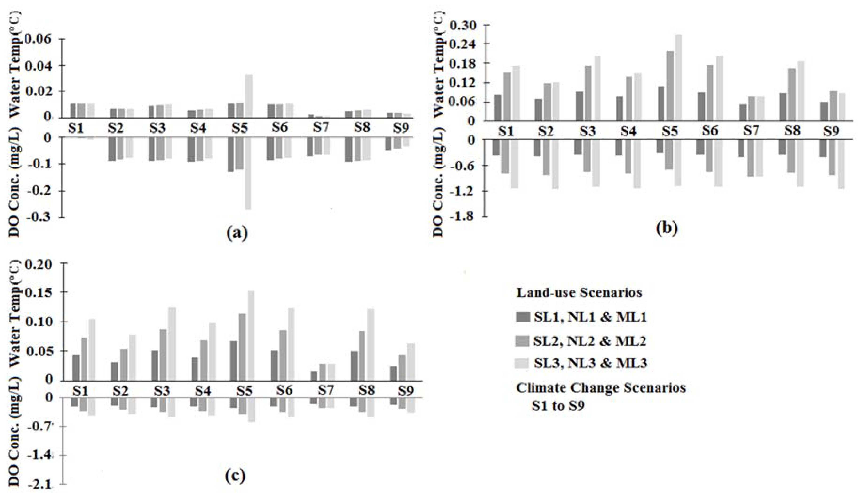
The effect of river catchment land-use on water temperature and DO concentrations are evaluated using three designed scenarios based on planned future development for three selected rivers. Figure 10a–c shows the result of the variability of DO levels and water temperatures due to land-use changes under different climate scenarios. In the Sengkang River, as agricultural land increases, the DO concentration and water temperature in the river decrease slightly.
A maximum increase of 0.03 °C in water temperature and a decrease of 0.27 mg/L in DO concentration is observed under future land-use scenarios at different climate change conditions using the existing land-use generated DO concentration, and water temperature mean values as benchmarks. It implies that conversion of forestlands to agricultural lands will not considerably affect the DO concentration and the water temperature under climate change conditions.
On the other hand, the Senai River shows a moderate variability in the water temperature and the DO concentration with a maximum increase of 0.25 °C and a decrease of 1.2 mg/L, respectively under future land-use scenarios. However, the Melana River shows a lower variability in both water temperature and DO concentration compared to the Senai River. It undergoes a maximum decrease of 0.5 mg/L in the DO concentration and maximum increase in the water temperature of 0.15 °C. However, the results show that land-use changes in the catchment of the river contribute to increases in water temperature and decreases as in DO concentration. Conversion of forest to built-up land will result in a substantial increase or decrease in water temperature and a substantial decrease in DO concentration compared to the conversion of forest to farmland. This means that an increase in urbanization will lead to an increase in river water temperature and a decrease in DO concentration in the future under the projected climate change. This situation will result in a distortion of the aquatic ecosystems and lead to water quality impairment in some of the local temporal rivers. However, rivers having agricultural or forest dominated drainage basins are expected to have a better ecological condition and accommodate most aquatic species independent of future climate changes.
4. Discussion
This study presents the impact of climate change on the water temperature and DO concentration in tropical rivers using basin-wide simulation. Rivers in the Skudai watershed in Malaysia were selected and subjected to nine climate change scenarios developed from the RegCM4 regional climate model. The RegCM4 model uses RCP 4.5 and 8.5 emission scenarios to project future climate change. In this study, we combined the two emission scenarios (RCP 4.5 and RCP 8.5) to developed nine climate change scenarios in which they were integrated to the calibrated water temperature and DO models of the Skudai watershed.
A sensitivity analysis of the model parameters was conducted to determine the significance that a single calibration parameter and input data have on the model result and to evaluate the uncertainty these parameters might have on the model output. We used perturbation analysis, and the result obtained shows that the correction factor for solar radiation (CFSEAX) parameter and the infiltration index (INFILT) parameter were the most sensitive parameters. The result obtained is similar to the result demonstrated by Cheng and Wiley [40]. They illustrate that stream temperature is more sensitive to solar radiation and depth. In our case, the infiltration index parameter (INFILT) determined the hydrological soil group and defined the in situ soil hydrologic conditions [37]. This means that the higher the infiltration rate, the less the runoff [52], and the river water depth decreases and hence influences the water temperature and DO concentration responses in the model calibration. Studies have shown that there is a good correlation between intensity precipitation and infiltration depth because water from a high-intensity rainfall event infiltrates more deeply compared with a low-intensity rainfall event [53].
The effect of increases in air temperature and variability in precipitation on the tropical rivers will change the water temperature conditions. The decrease in precipitation mostly influences likely changes in water temperature. The result of the statistical analysis shows that extreme climate change scenarios distinguish themselves from the mild climate scenarios. The result is in agreement with the result published in similar studies conducted by different climatic groups [18,54]. In addition, Lenderink and Van Meijgaard [55] show that changes in short-duration precipitation and temperature extremes can have significant impacts on the river system. The result of the post-hoc comparisons on the climate scenarios to their mean projected water temperatures shows that small changes in precipitation and air temperature produced similar mean water temperatures in tropical rivers.
Similarly, the impact of climate change on the DO concentration in the tropical rivers shows that DO concentrations declined in the tropical rivers in parallel with water temperature increase and a similar relationship has been discussed by others [15,56]. It was observed that the water temperature and DO concentration along the river section varied independently of climate variability. It was connected to the river channel condition, vegetation cover, hydrology, river physical properties, solar radiation and flow [57,58,59,60,61]. The mid-section and downstream portions of the rivers show a high resistance to climate change compared to the upstream section of the river. Because at the mid-section and downstream portions, the flow conditions are higher compared to the upstream and this is as a result of the contribution from the other tributary rivers that discharge into the main river which is mostly connected at the mid-section and the downstream parts. Woltemade [49] shows that quick changes in water temperature were associated with low discharge conditions and high flows influence low water temperature. The regression model developed from the relationship between streamflow and water temperature/DO concentration indicate a similar outcome. Because scenarios with tendencies to generate high streamflow produce low water temperature and high DO concentrations level compared with those scenarios that have strong tendencies to produced low streamflows. Besides, the correlation between water temperature and DO concentration in the tropical rivers are better under climate change scenarios with increased precipitation than those with decreased precipitation. It should be noted that changes of climate variables such as precipitation and temperature from the future climate projections will undoubtedly result in changes in streamflow, which also impacts water quality [51].
The predicted water temperature and DO concentration under the nine climate change scenarios indicate that tropical rivers have high resistance to climate change under the scenarios that show increased air temperature with increased precipitation but little resistance to climate change scenarios with low precipitation conditions and increased air temperature. This means that extreme scenarios are likely to affect water temperature and DO concentration in the tropical rivers. However, our studies reveal that the interaction between land-use and climate change can produce a different outcomes. It depends on the land-use composition and climate change scenarios [18]. Conversion of forest to built-up land resulted in an increase in water temperature and a decrease in the DO concentration compared to the conversion of forest to farmland. In the latter, the warmer water temperatures and lower DO concentrations might result in an increase in the nutrient flux and subsequently influences nutrient cycling [62]. In the former, it will reduce water temperature and increase the DO concentration. Thus, multiple stressors and climate change might change the prediction level of river water temperature and DO concentration in an agricultural dominated catchment [63]. However, in our case, we considered the conventional agricultural practices only in the study area and their impact are not considered in our scope of studies.
The projected mean DO concentration from the climate change scenarios indicates a DO level between 2.9 mg/L to 4.9 mg/L across the river system. However, a DO concentration level lower than 5.0 mg/L can put excessive stress on fish, and a DO concentration between 3 mg/L and 2 mg/L may result in fish kill [64]. Based on the common aquacultural practices (shrimp, climbing perch, and catfish) in the study area, the range of DO level and water temperature will not significantly affect the aquacultural species in the rivers. However, other environmental factors besides climate and land-use also control the long-term behavior of stream temperature [65], and these factors, which are not included in our study, might be detrimental to the ecosystem in which our study does not include. Future climate change indeed will impact the species composition of tropical rivers, leading to a dominance of warm water species that are able to adapt to a low DO concentration level and a consistently high water temperatures condition. As suggested by Hansen et al. [66], warm water species can quickly adapt to climate change compared to cold-water species. Understanding the effects of climate and predicting the effects of future climate change on water temperature and DO concentration on the river ecology is critical for effective resource management [67]. Thus, our results provide a basis in which significant management planning and mitigation actions can be taken.
5. Conclusions
This study demonstrates the likely impact of climate change on river water temperatures and DO concentrations in tropical rivers. Observed time series water temperature and DO concentration data for rivers in a Malaysian catchment area were used to calibrate a model using basin-wide simulation. The HSPF model was used to predict the impact of climate change on the stream water temperature and DO concentration. The results show that an increase in rainfall and air temperature will have little effect on water temperatures and DO concentrations as compared to a situation where an increase in air temperature and a decrease in rainfall occur. The latter will trigger higher water temperature and lower DO concentration. The relationships between streamflow, water temperatures and DO concentrations were evaluated, and they show that high to moderate streamflows lower water temperature and increase the DO concentration. Assessing the interaction between land-use changes in the river catchment on DO concentration and water temperature under different climate scenarios shows that land-use changes in the river catchment increase water temperatures and decrease DO concentrations. In addition, the land-use composition of the river catchment determines the water temperature and DO concentration changes in the river system. The impact of climate change and future development on the tropical rivers and how they might affect the future aquatic ecological system was briefly explained. As most rivers in suburban areas will be uninhabitable to most aquatic species as compared to agricultural and forest dominated rivers.
Acknowledgment
This research was supported by Malaysia Department of Irrigation and Drainage (DID), Department of Environment (DOE), and Indah Water Konsotium (IWK). We also wish to thank all the reviewers and editorial board whose insightful comments and suggestions significantly improved the quality of the manuscript.
Author Contributions
Al-Amin Danladi Bello designed the study, collected, and analyzed the data under the guidance of Noor Baharim Hashim and Mohd Ridza Mohd Haniffah. All the authors contributed substantially to the interpretation of results and editing the manuscript.
Conflicts of Interest
The authors declare no conflict of interest.
References
- Meyer, J.L.; Sale, M.J.; Mulholland, P.J.; Poff, N.L. Impacts of climate change on aquatic ecosystem functioning and health. JAWRA J. Am. Water Resour. Assoc. 1999, 35, 1373–1386. [Google Scholar] [CrossRef]
- Zeiger, S.; Hubbart, J.A.; Anderson, S.H.; Stambaugh, M.C. Quantifying and modelling urban stream temperature: A central US watershed study. Hydrol. Process. 2016, 30, 503–514. [Google Scholar] [CrossRef]
- Webb, B.W.; Clack, P.D.; Walling, D.E. Water-air temperature relationships in a Devon River system and the role of flow. Hydrol. Process. 2003, 17, 3069–3084. [Google Scholar] [CrossRef]
- Mohseni, O.; Stefan, H.G. Stream temperature/air temperature relationship: A physical interpretation. J. Hydrol. 1999, 218, 128–141. [Google Scholar] [CrossRef]
- Sinokrot, B.A.; Gulliver, J.S. In-stream flow impact on river water temperatures. J. Hydrol. Res. 2000, 38, 339–349. [Google Scholar] [CrossRef]
- Intergovernmental Panel on Climate Change. Climate Change 2014—Impacts, Adaptation and Vulnerability: Regional Aspects; Cambridge University Press: Cambridge, UK, 2014. [Google Scholar]
- Begum, R.A.; Siwar, C.; Abidin, R.D.Z.R.Z.; Pereira, J.J. Vulnerability of climate change and hardcore poverty in Malaysia. J. Environ. Sci. Technol. 2011, 4, 112–117. [Google Scholar] [CrossRef]
- Kavvas, M.L.; Chen, Z.Q.; Ohara, N.; Ahmad, J.; Amin, M. Study of the Impact of Climate Change on the Hydrologic Regime and Water Resources of Peninsular Malaysia; California Hydrologic Research Laboratory: San Diego, CA, USA, 2006. [Google Scholar]
- Colins, W.; Colman, R.; Haywood, J.; Manning, M.R.; Mote, P. The physical science behind climate change. Sci. Am. 2007, 297, 62–73. [Google Scholar] [CrossRef]
- Null, S.E.; Viers, J.H.; Deas, M.L.; Tanaka, S.K.; Mount, J.F. Stream temperature sensitivity to climate warming in California’s Sierra Nevada: Impacts to coldwater habitat. Clim. Chang. 2013, 116, 149–170. [Google Scholar] [CrossRef]
- Lee, K.H.; Cho, H.Y. Projection of climate-induced future water temperature for the aquatic environment. J. Environ. Eng. 2015, 141, 06015004. [Google Scholar] [CrossRef]
- Bayram, A.; Uzlu, E.; Kankal, M.; Dede, T. Modeling stream dissolved oxygen concentration using teaching-learning based optimization algorithm. Environ. Earth Sci. 2015, 73, 6565–6576. [Google Scholar] [CrossRef]
- El-Jabi, N.; Caissie, D.; Turkkan, N. Water quality index assessment under climate change. J. Water Resour. Prot. 2014, 6, 533. [Google Scholar] [CrossRef]
- Svendsen, M.B.S.; Bushnell, P.G.; Christensen, E.A.F.; Steffensen, J.F. Sources of variation in oxygen consumption of aquatic animals demonstrated by simulated constant oxygen consumption and respirometers of different sizes. J. Fish Biol. 2016, 88, 51–64. [Google Scholar] [CrossRef] [PubMed]
- Khani, S.; Rajaee, T. Modeling of Dissolved Oxygen Concentration and Its Hysteresis Behavior in Rivers Using Wavelet Transform-Based Hybrid Models. CLEAN Soil Air Water 2017. [Google Scholar] [CrossRef]
- Orr, H.G.; Simpson, G.L.; Clers, S.; Watts, G.; Hughes, M.; Hannaford, J.; Evans, R. Detecting changing river temperatures in England and Wales. Hydrol. Process. 2015, 29, 752–766. [Google Scholar] [CrossRef] [Green Version]
- Sun, N.; Yearsley, J.; Voisin, N.; Lettenmaier, D.P. A spatially distributed model for the assessment of land use impacts on stream temperature in small urban watersheds. Hydrol. Process. 2015, 29, 2331–2345. [Google Scholar] [CrossRef]
- Nelson, K.C.; Palmer, M.A. Stream temperature surges under urbanization and climate change: Data, models, and responses. JAWRA J. Am. Water Resour. Assoc. 2007, 43, 440–452. [Google Scholar] [CrossRef]
- Dudgeon, D. (Ed.) Tropical Stream Ecology; Academic Press: London, UK, 2011. [Google Scholar]
- Smith, P.; Gregory, P.J.; Van Vuuren, D.; Obersteiner, M.; Havlík, P.; Rounsevell, M.; Bellarby, J. Competition for land. Philos. Trans. R. Soc. Lond. B Biol. Sci. 2010, 365, 2941–2957. [Google Scholar] [CrossRef] [PubMed]
- Taniwaki, R.H.; Piggott, J.J.; Ferraz, S.F.; Matthaei, C.D. Climate change and multiple stressors in small tropical streams. Hydrobiologia 2017, 793, 41–53. [Google Scholar] [CrossRef]
- Pachauri, R.K.; Allen, M.R.; Barros, V.R.; Broome, J.; Cramer, W.; Christ, R.; Dubash, N.K. Climate Change 2014: Synthesis Report. Contribution of Working Groups I, II and III to the Fifth Assessment Report of the Intergovernmental Panel on Climate Change; IPCC: Geneva, Switzerland, 2014. [Google Scholar]
- Hamdan, O.; Aziz, H.K.; Hasmadi, I.M. L-band ALOS PALSAR for biomass estimation of Matang Mangroves, Malaysia. Remote Sens. Environ. 2014, 155, 69–78. [Google Scholar] [CrossRef]
- Pour, A.B.; Hashim, M. Identification of High Potential Bays for HABs occurrence in Peninsular Malysia using Palsar Remote Sensing Data. Int. Arch. Photogramm. Remote Sens. Spat. Inf. Sci. 2016, 42, 97–101. [Google Scholar] [CrossRef]
- Chen, D.; Hu, M.; Guo, Y.; Dahlgren, R.A. Changes in river water temperature between 1980 and 2012 in Yongan watershed, eastern China: Magnitude, drivers and models. J. Hydrol. 2016, 533, 191–199. [Google Scholar] [CrossRef]
- Mora, C.; Frazier, A.G.; Longman, R.J.; Dacks, R.S.; Walton, M.M.; Tong, E.J.; Ambrosino, C.M. The projected timing of climate departure from recent variability. Nature 2013, 502, 183–187. [Google Scholar] [CrossRef] [PubMed]
- Shahid, S.; Pour, S.H.; Pour, S.H.; Wang, X.; Wang, X.; Ismail, T.B. Impacts and adaptation to climate change in Malaysian real estate. Int. J. Clim. Chang. Strateg. Manag. 2017, 9, 87–103. [Google Scholar] [CrossRef]
- Wong, C.L.; Venneker, R.; Uhlenbrook, S.; Jamil, A.B.M.; Zhou, Y. Variability of rainfall in Peninsular Malaysia. Hydrol. Earth Syst. Sci. Discuss. 2009, 6, 5471–5503. [Google Scholar] [CrossRef]
- Paramananthan, S. Soils of Malaysia: Their Characteristics and Identification; Academy of Sciences Malaysia: Kuala Lumpur, Malaysia, 2000.
- Malone, R.W.; Yagow, G.; Baffaut, C.; Gitau, M.W.; Qi, Z.; Amatya, D.M.; Green, T.R. Parameterization guidelines and considerations for hydrologic models. Trans. ASABE 2015, 58, 1681–1703. [Google Scholar]
- Daniel, E.B.; Camp, J.V.; LeBoeuf, E.J.; Penrod, J.R.; Abkowitz, M.D.; Dobbins, J.P. Watershed modeling using GIS technology: A critical review. J. Spat. Hydrol. 2011, 10, 2. [Google Scholar]
- Bicknell, B.R.; Imhoff, J.C.; Kittle, J.L., Jr.; Jobes, T.H.; Donigian, A.S., Jr.; Johanson, R. Hydrological Simulation Program—Fortran: HSPF, Version 12 User’s Manual; EPA National Exposure Research Laboratory: Athens, GA, USA, 2001.
- Donigian, A.S.; Crawford, N.H. Modeling Nonpoint Pollution from the Land Surface; US Environmental Protection Agency: Athens, GA, USA, 1976.
- Juneng, L.; Tangang, F.; Chung, J.X.; Ngai, S.T.; Tay, T.W.; Narisma, G.; Singhruck, P. Sensitivity of Southeast Asia rainfall simulations to cumulus and air-sea flux parameterizations in regCM4. Clim. Res. 2016, 69, 59–77. [Google Scholar] [CrossRef]
- AQUA TERRA Consultants. Available online: http://www.aquaterra.com/resources/downloads/HSPEXPplus.php (accessed on 15 November 2016).
- Moriasi, D.N.; Arnold, J.G.; Van Liew, M.W.; Bingner, R.L.; Harmel, R.D.; Veith, T.L. Model evaluation guidelines for systematic quantification of accuracy in watershed simulations. Trans. ASABE 2007, 50, 885–900. [Google Scholar] [CrossRef]
- Diaz-Ramirez, J.N.; McAnally, W.H.; Martin, J.L. Sensitivity of simulating hydrologic processes to gauge and radar rainfall data in subtropical coastal catchments. Water Resour. Manag. 2012, 26, 3515–3538. [Google Scholar] [CrossRef]
- Gardner, R.H.; O’neill, R.V.; Mankin, J.B.; Carney, J.H. A comparison of sensitivity analysis and error analysis based on a stream ecosystem model. Ecol. Model. 1981, 12, 173–190. [Google Scholar] [CrossRef]
- Gelaro, R.; Buizza, R.; Palmer, T.N.; Klinker, E. Sensitivity analysis of forecast errors and the construction of optimal perturbations using singular vectors. J. Atmos. Sci. 1998, 55, 1012–1037. [Google Scholar] [CrossRef]
- Cheng, S.T.; Wiley, M.J. A Reduced Parameter Stream Temperature Model (RPSTM) for basin-wide simulations. Environ. Model. Softw. 2016, 82, 295–307. [Google Scholar] [CrossRef]
- Hunt, R.J.; Westenbroek, S.M.; Walker, J.F.; Selbig, W.R.; Regan, R.S.; Leaf, A.T.; Saad, D.A. Simulation of Climate Change Effects on Streamflow, Groundwater, and Stream Temperature Using GSFLOW and SNTEMP in the Black Earth Creek Watershed, Wisconsin; US Geological Survey: Reston, VA, USA, 2016.
- Imhoff, J.C.; Kittle, J.L.; Gray, M.R.; Johnson, T.E. Using the climate assessment tool (CAT) in US EPA BASINS integrated modeling system to assess watershed vulnerability to climate change. Water Sci. Technol. 2007, 56, 49–56. [Google Scholar] [CrossRef] [PubMed]
- Su, Q.; Cai, G.; Degée, H. Application of Variance Analyses Comparison in Seismic Damage Assessment of Masonry Buildings Using Three Simplified Indexes. Math. Probl. Eng. 2017, 2017, 3741941. [Google Scholar] [CrossRef]
- Anderson, M.J. A new method for non-parametric multivariate analysis of variance. Austral Ecol. 2001, 26, 32–46. [Google Scholar]
- Johnson, H.E.; Kular, B.; Mur, L.; Smith, A.R.; Wang, T.L.; Causton, D.R. The application of multivariate analysis of variance (MANOVA) to evaluate plant metabolomic data from factorially designed experiments. Metabolomics 2016, 12, 191. [Google Scholar] [CrossRef]
- Harvey, R.; Lye, L.; Khan, A.; Paterson, R. The Influence of air temperature on water temperature and the concentration of dissolved oxygen in Newfoundland Rivers. Can. Water Resour. J. 2011, 36, 171–192. [Google Scholar] [CrossRef]
- Woltemade, C.J.; Hawkins, T.W. Stream temperature impacts because of changes in air temperature, Land cover and stream discharge: Navarro River watershed, California, USA. River Res. Appl. 2016, 32, 2020–2031. [Google Scholar] [CrossRef]
- Leach, J.A.; Olson, D.H.; Anderson, P.D.; Eskelson, B.N.I. Spatial and seasonal variability of forested headwater stream temperatures in western Oregon, USA. Aquat. Sci. 2017, 79, 291–307. [Google Scholar] [CrossRef]
- Woltemade, C.J. Stream temperature spatial variability reflects geomorphology, hydrology, and microclimate: Navarro River watershed, California. Prof. Geogr. 2017, 69, 177–190. [Google Scholar] [CrossRef]
- Baroni, G.; Tarantola, S. A General Probabilistic Framework for uncertainty and global sensitivity analysis of deterministic models: A hydrological case study. Environ. Model. Softw. 2014, 51, 26–34. [Google Scholar] [CrossRef]
- Gibson, C.A.; Meyer, J.L.; Poff, N.L.; Hay, L.E.; Georgakakos, A. Flow regime alterations under changing climate in two river basins: Implications for freshwater ecosystems. River Res. Appl. 2005, 21, 849–864. [Google Scholar] [CrossRef]
- Mishra, A.; Kar, S.; Singh, V.P. Determination of runoff and sediment yield from a small watershed in sub-humid subtropics using the HSPF model. Hydrol. Process. 2007, 21, 3035–3045. [Google Scholar] [CrossRef]
- Sala, O.E.; Lauenroth, W.K.; Parton, W.J.; Trlica, M.J. Water status of soil and vegetation in a shortgrass steppe. Oecologia 1981, 48, 327–331. [Google Scholar] [CrossRef] [PubMed]
- Fang, X.; Stefan, H.G. Simulation of climate effects on water temperature, dissolved oxygen, and ice and snow covers in lakes of the contiguous US under past and future climate scenarios. Limnol. Oceanogr. 2009, 54, 2359–2370. [Google Scholar] [CrossRef]
- Lenderink, G.; Van Meijgaard, E. Increase in hourly precipitation extremes beyond expectations from temperature changes. Nat. Geosci. 2008, 1, 511–514. [Google Scholar] [CrossRef]
- Tang, C.; Li, Y.; Jiang, P.; Yu, Z.; Acharya, K. A coupled modeling approach to predict water quality in Lake Taihu, China: Linkage to climate change projections. J. Freshw. Ecol. 2015, 30, 59–73. [Google Scholar] [CrossRef]
- Isaak, D.J.; Wollrab, S.; Horan, D.; Chandler, G. Climate change effects on stream and river temperatures across the northwest US from 1980–2009 and implications for salmonid fishes. Clim. Chang. 2012, 113, 499–524. [Google Scholar] [CrossRef]
- Flint, L.E.; Flint, A.L. A basin-scale approach to estimating stream temperatures of tributaries to the Lower Klamath River, California. J. Environ. Qual. 2008, 37, 57–68. [Google Scholar] [CrossRef] [PubMed]
- Caissie, D. The thermal regime of rivers: A review. Freshw. Biol. 2006, 51, 1389–1406. [Google Scholar] [CrossRef]
- Meier, W.; Bonjour, C.; Wüest, A.; Reichert, P. Modeling the effect of water diversion on the temperature of mountain streams. J. Environ. Eng. 2003, 129, 755–764. [Google Scholar] [CrossRef]
- Gaffield, S.J.; Potter, K.W.; Wang, L. Predicting the summer temperature of small streams in southwestern Wisconsin. JAWRA J. Am. Water Resour. Assoc. 2005, 41, 25–36. [Google Scholar] [CrossRef]
- Taner, M.Ü.; Carleton, J.N.; Wellman, M. Integrated model projections of climate change impacts on a North American lake. Ecol. Model. 2011, 222, 3380–3393. [Google Scholar] [CrossRef]
- Piggott, J.J.; Townsend, C.R.; Matthaei, C.D. Climate warming and agricultural stressors interact to determine stream macroinvertebrate community dynamics. Glob. Chang. Biol. 2015, 21, 1887–1906. [Google Scholar] [CrossRef] [PubMed]
- Leuven, R.S.E.W.; Hendriks, A.J.; Huijbregts, M.A.J.; Lenders, H.J.R.; Matthews, J.; Van der Velde, G. Differences in sensitivity of native and exotic fish species to changes in river temperature. Curr. Zool. 2011, 57, 852–862. [Google Scholar] [CrossRef]
- Kaushal, S.S.; Likens, G.E.; Jaworski, N.A.; Pace, M.L.; Sides, A.M.; Seekell, D.; Wingate, R.L. Rising stream and river temperatures in the United States. Front. Ecol. Environ. 2010, 8, 461–466. [Google Scholar] [CrossRef]
- Hansen, G.J.; Read, J.S.; Hansen, J.F.; Winslow, L.A. Projected shifts in fish species dominance in Wisconsin lakes under climate change. Glob. Chang. Biol. 2017, 23, 1463–1476. [Google Scholar] [CrossRef] [PubMed]
- Heller, N.E.; Zavaleta, E.S. Biodiversity management in the face of climate change: A review of 22 years of recommendations. Biol. Conserv. 2009, 142, 14–32. [Google Scholar] [CrossRef]
Figure 1.
(a) Location of the study area; (b) stations and elevation details; and (c) land-use class distribution.
Figure 1.
(a) Location of the study area; (b) stations and elevation details; and (c) land-use class distribution.

Figure 2.
(a) Projected climate change for Skudai watershed from regional climate model (RegCM4) under RCP 4.5 and 8.5 scenarios for air temperature; and (b) projected climate change for Skudai watershed from RegCM4 model under RCP 4.5 and 8.5 scenarios for precipitation.
Figure 2.
(a) Projected climate change for Skudai watershed from regional climate model (RegCM4) under RCP 4.5 and 8.5 scenarios for air temperature; and (b) projected climate change for Skudai watershed from RegCM4 model under RCP 4.5 and 8.5 scenarios for precipitation.

Figure 3.
The calibrated and validated streamflow (m3/s) at monthly time step for Skudai watershed.

Figure 4.
Plot of the observed and simulated water temperature and DO concentration: (a) station 3S110; (b) station 3S117; and (c) station 3S116.
Figure 4.
Plot of the observed and simulated water temperature and DO concentration: (a) station 3S110; (b) station 3S117; and (c) station 3S116.
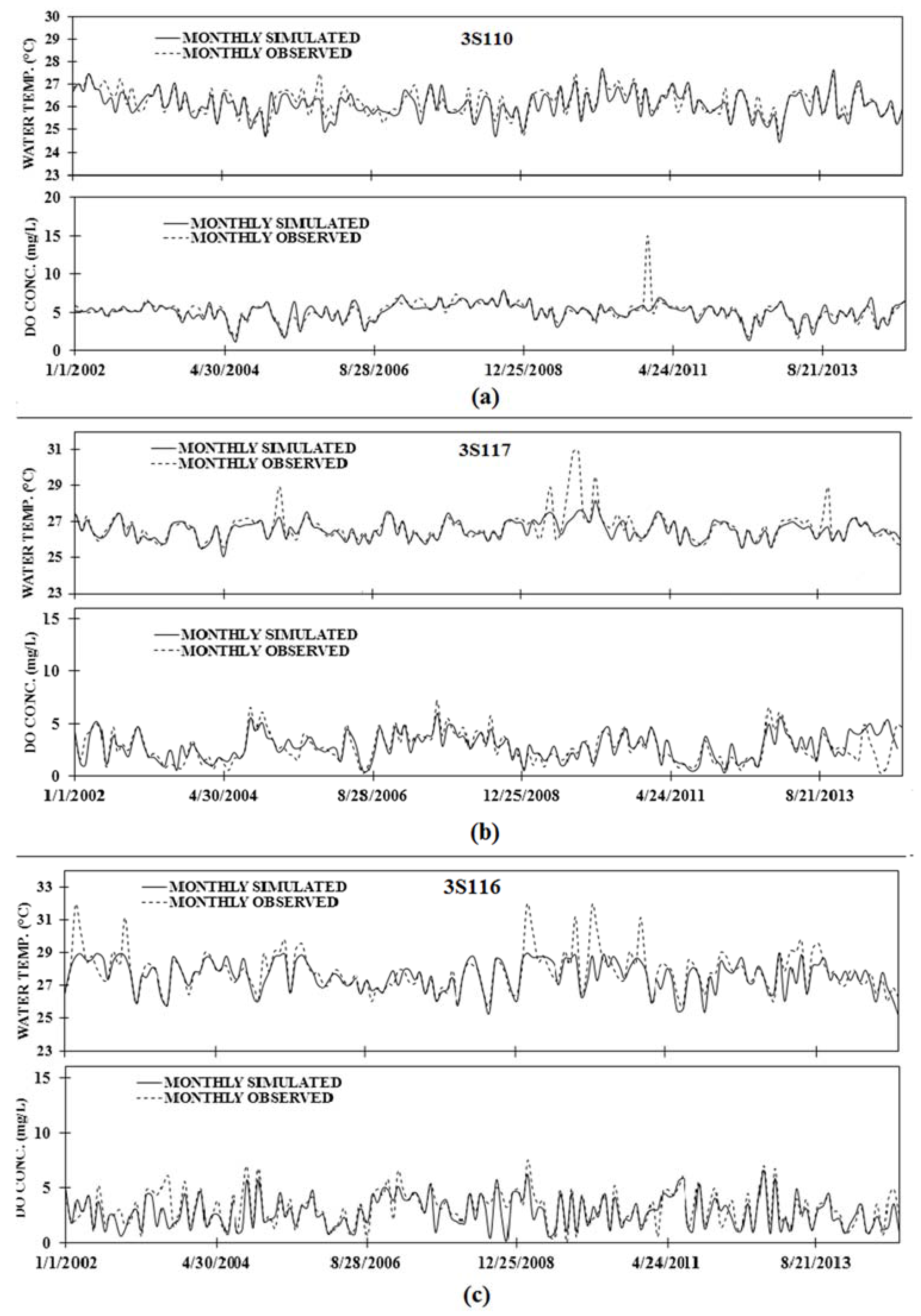
Figure 5.
Graphical representation of the sensitivity analysis performed at the three stations to determine the relative influence of each parameter based on the modeled mean water temperature and DO concentration in the period from 2002 to 2014: (a) station 3S110; (b) station 3S117; and (c) station 3S116.

Figure 6.
Mean water temperatures for climate change scenarios with the columns labeled from one to six denoting homogenous subsets of scenarios: (a) upstream (b) mid-section (c) downstream
Figure 6.
Mean water temperatures for climate change scenarios with the columns labeled from one to six denoting homogenous subsets of scenarios: (a) upstream (b) mid-section (c) downstream
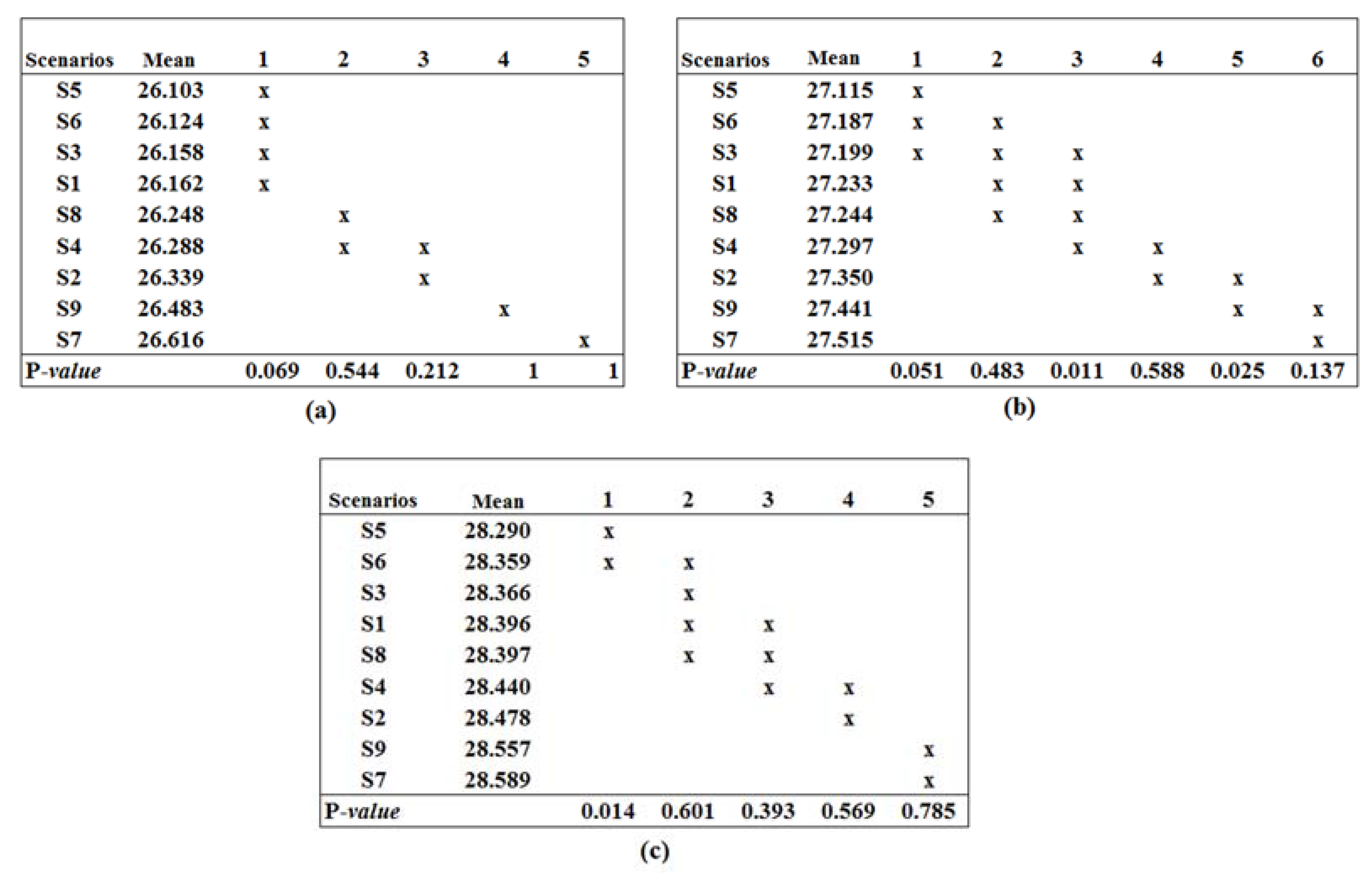
Figure 7.
Mean dissolved oxygen (DO) concentrations for climate change scenarios with the columns labeled from 1 to 6 denoting homogenous subset of scenarios: (a) upstream (b) mid-section (c) downstream.
Figure 7.
Mean dissolved oxygen (DO) concentrations for climate change scenarios with the columns labeled from 1 to 6 denoting homogenous subset of scenarios: (a) upstream (b) mid-section (c) downstream.

Figure 8.
Correlation plot between simulated water temperature and dissolved oxygen concentration under different climate change scenarios (red lines represent the polynomial regression and blue lines represent the exponential regression): (a) S1 (b) S2 (c) S3 (d) S4 (e) S5 (f) S6 (g) S7 (h) S8 (i) S9.

Figure 9.
Correlation plot for streamflow versus water temperature (blue lines) and stream flow versus dissolve oxygen concentration (red lines) for all the climate change scenarios: (a) S1 (b) S2 (c) S3 (d) S4 (e) S5 (f) S6 (g) S7 (h) S8 (i) S9.
Figure 9.
Correlation plot for streamflow versus water temperature (blue lines) and stream flow versus dissolve oxygen concentration (red lines) for all the climate change scenarios: (a) S1 (b) S2 (c) S3 (d) S4 (e) S5 (f) S6 (g) S7 (h) S8 (i) S9.
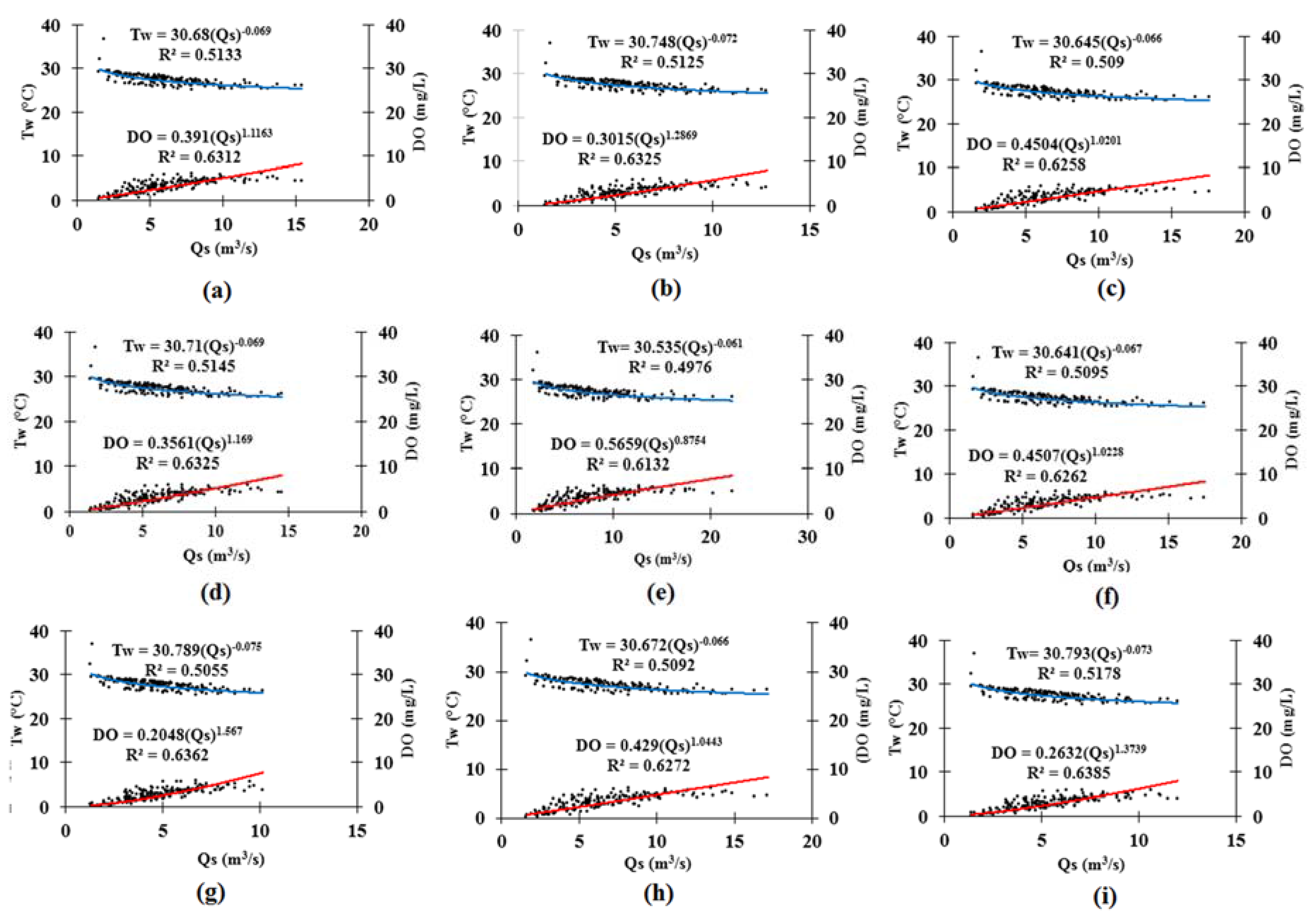
Figure 10.
Interactions between land-use and climate change on three small tropical rivers and their impacts on water temperature and DO concentration: (a) Sengkang River; (b) Senai River; and (c) Melana River.
Figure 10.
Interactions between land-use and climate change on three small tropical rivers and their impacts on water temperature and DO concentration: (a) Sengkang River; (b) Senai River; and (c) Melana River.

Table 1.
Characteristics of the major rivers in the study area.
| Names of Rivers | Soil Texture | Drainage Area (km2) | Length of the Rivers (km) | Average Slope (%) | Land-Use Composition of the River Catchment (%) | ||||
|---|---|---|---|---|---|---|---|---|---|
| Built-up | Agriculture | Forest | Wetland | Barren Land | |||||
| Sengkang | Sandy loam | 11.7 | 4.0 | 10.7 | 2.9 | 9.5 | 85.5 | 0.0 | 2.1 |
| Senai | Sand Silty Clay | 30.4 | 11.8 | 11.4 | 8.2 | 20.5 | 69.5 | 0.1 | 1.7 |
| Melana | Sand Silty Clay | 44.3 | 18.7 | 9.6 | 55.3 | 23.8 | 19.4 | 1.5 | 0.0 |
| Danga | Sand Silty Clay | 18.1 | 12.2 | 20.3 | 57.7 | 28.1 | 11.1 | 3.1 | 0.0 |
| Skudai | Sandy Clay | 182.9 | 42.8 | 11.7 | 44.5 | 31.9 | 21.1 | 1.9 | 0.6 |
Table 2.
Model parameters/input data used for Sensitivity Analysis.
| Notation | Definition | Typical Range of Calibration Values | Max. No. of Calibration Values |
|---|---|---|---|
| LZSN | Lower zone nominal soil moisture storage | 2.0–15.0 | 100 |
| INFILT | Index to infiltration capacity | 0.001–0.5 | 100 |
| UZSN | Upper zone nominal soil moisture storage | 0.05–2.0 | 10 |
| INFTW | Interflow inflow parameter | 1.0–10.0 | - |
| AIR TEMP | Air temperature | - | - |
| PREC | Precipitation | - | - |
| KEVAP | Evaporation coefficient | 0.001–10 | 10 |
| KCOND | Conduction-convection heat transport coefficient | 0.001–20 | 20 |
| KATRAD | Long wave radiation coefficient | 0.001–20 | 20 |
| CFSAEX | Correction factor for solar radiation | 0.001–2.0 | 2 |
Table 3.
Change in temperature and precipitation for each designed climate scenarios with their monthly average.
Table 3.
Change in temperature and precipitation for each designed climate scenarios with their monthly average.
| Scenarios | Description | Base Year | Monthly Prec. (mm) | Monthly Temp. (°C) | Prec. & Temp Anomaly | |||
|---|---|---|---|---|---|---|---|---|
| Min. | Max. | Min. | Max. | Prec. (%) | Temp. (°C) | |||
| S1 | Baseline | 2000 | 56.5 | 260.6 | 24.6 | 26.3 | 0 | 0 |
| S2 | Early century (RCP 4.5) | 2030 | 65.8 | 183.3 | 24.9 | 26.6 | −15.4 | 0.6 |
| S3 | Mid Century (RCP 4.5) | 2050 | 89.7 | 246.5 | 25.3 | 27.2 | 11.6 | 1.0 |
| S4 | Near End Century (RCP 4.5) | 2070 | 26.9 | 281.9 | 25.8 | 27.5 | −4.6 | 1.2 |
| S5 | End Century (RCP 4.5) | 2090 | 65.4 | 702.5 | 26.3 | 27.9 | 36.9 | 1.9 |
| S6 | Early century (RCP 8.5) | 2030 | 71.2 | 320.8 | 25.1 | 26.4 | 11.2 | 0.5 |
| S7 | Mid Century (RCP 8.5) | 2050 | 26.7 | 271.7 | 25.8 | 27.5 | −34.4 | 1.4 |
| S8 | Near End Century (RCP 8.5) | 2070 | 23.4 | 355.2 | 26.2 | 28.1 | 9.0 | 2.0 |
| S9 | End Century (RCP 8.5) | 2090 | 39.9 | 256.9 | 26.6 | 28.2 | −24.2 | 2.5 |
Table 4.
Rivers and Surrounding Land-use scenarios.
| Names of Rivers | Scenarios | Changes in Land-Use Composition within the River Catchment (%) | ||||
|---|---|---|---|---|---|---|
| Built-Up | Agriculture | Forest | Wetland | Barren Land | ||
| Sengkang | SL1 | 5.0 | 25.0 | 65.0 | 0.0 | 5.0 |
| SL2 | 5.0 | 50.0 | 40.0 | 0.0 | 5.0 | |
| SL3 | 5.0 | 75.0 | 15.0 | 0.0 | 5.0 | |
| Senai | NL1 | 25.0 | 20.0 | 53.2 | 0.1 | 1.7 |
| NL2 | 50.0 | 20.0 | 28.2 | 0.1 | 1.7 | |
| NL3 | 75.0 | 20.0 | 3.2 | 0.1 | 1.7 | |
| Melana | ML1 | 75.0 | 15.0 | 8.5 | 1.5 | 0.0 |
| ML2 | 85.0 | 10.0 | 3.5 | 1.5 | 0.0 | |
| ML3 | 95.0 | 3.0 | 0.5 | 1.5 | 0.0 | |
Table 5.
Hydrological Simulation Program FORTRAN (HSPF) model Performance Statistics (Hydrology).
| Statistical Model | Calibration | Validation |
|---|---|---|
| Coefficient of determination (R2) | 0.89 | 0.83 |
| Nash–Sutcliffe Efficiency (NSE) | 0.88 | 0.82 |
| Percent bias (PBIAS) | −6.28 | −3.91 |
Table 6.
Statistical measurement of calibrated water temperature (Tw) and Dissolved Oxygen (DO).
| Statistical Parameters | 3S110 | 3S117 | 3S116 | |||
|---|---|---|---|---|---|---|
| Tw | DO | Tw | DO | Tw | DO | |
| Average Monthly Values | ||||||
| Observed (in °C or mg/L) | 26.20 | 5.13 | 26.68 | 2.80 | 27.66 | 3.19 |
| Simulated (in °C or mg/L) | 26.18 | 4.99 | 26.66 | 2.87 | 27.62 | 2.84 |
| Standard Deviation | ||||||
| Observed | 0.59 | 1.38 | 0.71 | 1.45 | 0.95 | 1.62 |
| Simulated | 0.62 | 1.18 | 0.68 | 1.32 | 0.90 | 1.48 |
| Performance Statistics | ||||||
| T-test | 0.94 | 1.88 | 1.60 | −0.89 | 1.84 | 3.44 |
| p-Value | 0.34 | 0.06 | 0.11 | 0.38 | 0.07 | 0.04 |
| Correlation coefficient | 0.86 | 0.75 | 0.98 | 0.79 | 0.86 | 0.81 |
| Coefficient of determination R2 | 0.74 | 0.55 | 0.70 | 0.62 | 0.64 | 0.65 |
| Nash–Sutcliffe efficiency (NSE) | 0.70 | 0.53 | 0.64 | 0.60 | 0.60 | 0.59 |
| Percent Bias (PBIAS) | 0.09 | 2.72 | 0.55 | −2.31 | 0.84 | 10.80 |
Table 7.
Comparison of the results of one-way ANOVA (water temperature).
| Skudai Rivers Section | Sources | d.f | Sum of Square | Mean Square | F-Statistics | p-Value |
|---|---|---|---|---|---|---|
| Upstream | Scenarios | 1377.0 | 8.0 | 172.1 | 151.6 | 0.0 |
| Residual | 57,791.0 | 50,914.0 | 1.1 | |||
| Total | 59,168.0 | 50,922.0 | ||||
| Mid-section | Scenarios | 745.8 | 8.0 | 93.2 | 44.2 | 0.0 |
| Residual | 107,509.3 | 50,914.0 | 2.1 | |||
| Total | 108,255.1 | 50,922.0 | ||||
| Downstream | Scenarios | 421.5 | 8.0 | 52.7 | 48.4 | 0.0 |
| Residual | 55,376.7 | 50,914.0 | 1.1 | |||
| Total | 55,798.1 | 50,922.0 |
Table 8.
Comparison of the results of one-way ANOVA (DO concentration).
| Skudai Rivers Section | Sources | d.f | Sum of Square | Mean Square | F-Statistics | p-Value |
|---|---|---|---|---|---|---|
| Upstream | Scenarios | 1672.5 | 8.0 | 209.1 | 121.9 | 0.0 |
| Residual | 87,282.1 | 50,913.0 | 1.7 | |||
| Total | 88,954.6 | 50,921.0 | ||||
| Mid-section | Scenarios | 3254.4 | 8.0 | 406.8 | 135.3 | 0.0 |
| Residual | 153,042.1 | 50,913.0 | 3.0 | |||
| Total | 156,296.5 | 50,921.0 | ||||
| Downstream | Scenarios | 1854.6 | 8.0 | 231.8 | 90.0 | 0.0 |
| Residual | 131,153.9 | 50,913.0 | 2.6 | |||
| Total | 133,008.5 | 50,921.0 |
© 2017 by the authors. Licensee MDPI, Basel, Switzerland. This article is an open access article distributed under the terms and conditions of the Creative Commons Attribution (CC BY) license (http://creativecommons.org/licenses/by/4.0/).
Share and Cite
MDPI and ACS Style
Danladi Bello, A.-A.; Hashim, N.B.; Mohd Haniffah, M.R. Predicting Impact of Climate Change on Water Temperature and Dissolved Oxygen in Tropical Rivers. Climate 2017, 5, 58. https://doi.org/10.3390/cli5030058
AMA Style
Danladi Bello A-A, Hashim NB, Mohd Haniffah MR. Predicting Impact of Climate Change on Water Temperature and Dissolved Oxygen in Tropical Rivers. Climate. 2017; 5(3):58. https://doi.org/10.3390/cli5030058
Chicago/Turabian StyleDanladi Bello, Al-Amin, Noor Baharim Hashim, and Mohd Ridza Mohd Haniffah. 2017. "Predicting Impact of Climate Change on Water Temperature and Dissolved Oxygen in Tropical Rivers" Climate 5, no. 3: 58. https://doi.org/10.3390/cli5030058
Note that from the first issue of 2016, this journal uses article numbers instead of page numbers. See further details here.