
Influence of Parameter Sensitivity and Uncertainty on Projected Runoff in the Upper Niger Basin under a Changing Climate


1
Department of Soil Science, Faculty of Agriculture, University of Abuja, Abuja 900211, Nigeria
2
Department of Geography, University of Bonn, Meckenheimer Allee 166, Bonn 53115, Germany
*
Author to whom correspondence should be addressed.
Climate 2017, 5(3), 67; https://doi.org/10.3390/cli5030067
Submission received: 2 June 2017
/
Revised: 21 August 2017
/
Accepted: 23 August 2017
/
Published: 27 August 2017
(This article belongs to the Special Issue Modified Hydrological Cycle under Global Warming)
Abstract
:Hydro-climatic projections in West Africa are attributed with high uncertainties that are difficult to quantify. This study assesses the influence of the parameter sensitivities and uncertainties of three rainfall runoff models on simulated discharge in current and future times using meteorological data from eight Global Climate Models (GCM). The IHACRES Catchment Moisture Deficit (IHACRES-CMD) model, the GR4J, and the Sacramento model were chosen for this study. During the model evaluation, 10,000 parameter sets were generated for each model and used in a sensitivity and uncertainty analysis using the Generalized Likelihood Uncertainty Estimation (GLUE) method. Out of the three models, IHACRES-CMD recorded the highest Nash-Sutcliffe Efficiency (NSE) of 0.92 and 0.86 for the calibration (1997–2003) and the validation (2004–2010) period, respectively. The Sacramento model was able to adequately predict low flow patterns on the catchment, while the GR4J and IHACRES-CMD over and under estimated low flow, respectively. The use of multiple hydrological models to reduce uncertainties caused by model approaches is recommended, along with other methods for sustainable river basin management.
1. Introduction
Many uncertainties are associated with climate predictions in West Africa [1]. This is attributed to the complexity of the regional climate and the influence of regional geographic features, such as deserts, land cover variations, mountain chains, large lakes, land-sea contrasts, and the sea surface temperatures (SSTs) of the adjacent ocean [2]. Climate patterns in the historical periods are not properly documented [3] and satellite-based observations have been identified with inherent biases [2]. This has led to contradictory results from climate trend studies at local and sub-regional scales [4]. The Niger River Basin, the largest basin in West Africa and the main water source of the Sahel, was also ascribed with challenging uncertainties for hydrological predictions caused by climate and land use change [5]. A vivid example is the “Sahelian paradox”, which is an observed runoff increase in some Sahelian catchments of the Niger basin, such as in Nakanbe (Burkina Faso), Sirba (Niger), and Mekrou (Benin), despite a decrease in rainfall [6,7].
Rainfall runoff (RR) models are widely used tools in hydrology because of the simplicity in their usage and the required input data are readily available for most applications [8]. More complex, physically-based, distributed models often require input data such as soil and land use data that are either missing or weakly reliable in West Africa [9]. However, the results of any modelling exercise are uncertain due to different reasons [10]. Characterization of the uncertainties affecting RR models remains a major scientific and operational challenge. Vetter et al. [11] concluded that scenarios from climate models are the largest uncertainty source, providing large discrepancies in precipitation, and therefore hydrological projections often do not show a clear trend. Renard et al. [12] ascribed uncertainties in RR models to either input data or model structure. Data uncertainty stems from sampling, measurement, and interpretation errors in the observed input/output data. Since these errors arise independently from the RR model, their properties (e.g., means and variances of rainfall and runoff errors) can be estimated prior to the calibration by analysing data acquisition instruments and procedures [12]. Structural uncertainties are an inherent feature of all hydrological models including RR models. It is a consequence of simplifying assumptions made in approximating the actual environmental system by a mathematical function [12].
In West Africa, several authors have evaluated uncertainties in climate [2,13,14] and runoff [11,15] modelling. While most authors stopped at the assessment of only climate uncertainties, Cornelissen et al. [15] used three distributed and semi distributed models along with a RR model to project climate and land use change impacts in Benin. The authors observed differences in the robustness of the models to simulate the current total discharge and its components. They attributed these differences to serious uncertainties in the input data, particularly in the precipitation and saturated hydraulic conductivity data, calibration strategy, parameterization, and differences in model structure. In their study, Cornelissen et al. [15] only used climate scenarios from one Regional Climate Model (RCM) which limits their finding concerning uncertainties in future climate change impacts. Yira et al. [16] used six different RCM-GCM combinations to study climate change impacts on water resources of a 200 km² catchment in Burkina Faso. They found that the different climate models do not show a clear trend; whilst some are predicting a wetter future, others are predicting a drier one. Therefore, a clear trend is missing because of the complex West African climate system [2]. Despite the above highlighted studies on hydro-climatic uncertainties in West Africa, only a few studies have evaluated the effects of combining multi climate and hydrological models on current and future hydroclimatic projections in the Niger basin. This will give more information on interactions between climate and hydrological model uncertainties and their impacts on projected runoff. This study aims to assess future runoff projections in the upper Niger basin by using multiple climate and hydrological models. Parameter sensitivities and uncertainties of three hydrological models were evaluated in terms of their influence on the projected runoff from climate data of eight GCM.
2. Materials and Methods
2.1. Study Area
The Niger River Basin covers 2.27 million km2, with the active drainage area comprising less than 50% of the total basin [17]. Being 4200 km in length, it is the third longest river in Africa and the world’s ninth largest river system. The study area is the Upper Niger catchment at the Koulikoro gauging station, Mali (Figure 1), covering an area of about 120,000 km2. It spreads over the countries of Guinea and Mali, and a small part of the Côte d’Ivoire. According to Vetter et al. [11], the topography of the catchment is quite heterogeneous, with several steep-sloped tributaries in the Upper Guinea that flow into the floodplain of the Niger River. The dominant land cover in the Upper Niger catchment is forest (34%), followed by savannah (30%). The climate is characterized by a dry season (November–May) and a rainy season from June to September. Rainfall that feeds the river mainly comes from the Guinean Highlands during the rainy season. It has an average annual precipitation of 1495 mm and the catchment is not significantly influenced by human management. There are no major irrigation schemes in this part of the Niger basin [11].
2.2. Modelling Framework
2.2.1. Hydrological Models
The selected models are included in the R package “Hydromad” [18]. The three rainfall-runoff models estimate the streamflow at a catchment outlet using inputs of areal rainfall and potential evapotranspiration (PET) at daily time steps. The first model is the IHACRES-CMD model with a two store routing component [18,19]. The second is the Sacramento model [18,20], and the third model is the GR4J model which has a production and routing store [21]. While the IHACRES-CMD model has three soil moisture accounting parameters (Table 1), the GR4J model has four parameters, and the Sacramento model has thirteen parameters (Table 1). IHACRES-CMD and GR4J were selected due to their wide usage and acceptability in hydrological studies in the Niger basin [9,22,23,24]. The Sacramento model was added to the two well-known models in the region because of its robust parameterisation. Optimum model parameters for all the models were obtained by an automatic calibration with the “fitByOptim” algorithm on R [18], which selects the optimum parameters that give the best preferred model performance statistics—here taken as the Nash-Sutcliffe Efficiency. The observed and simulated runoff was compared using the following efficiency coefficients which were selected due to their wide usage and acceptability in the region: Nash-Sutcliffe Efficiency (∞ < NSE ≤ 1) [25], Mean Error (ME) [26], Root Mean Squared Error (RMSE) [27], Ratio of Standard Deviations (RSD) [26], Volumetric Efficiency (VE) [28], and Kling-Gupta Efficiency (0 ≤ KGE ≤ 1) [29].
NSE is commonly used to assess the predictive power of hydrological discharge models. It is defined as:
where O is the observed value and S is the simulated value at day i.
An efficiency of 1 corresponds to a perfect match between the model and observations. The mean error ME refers to the average of all the errors in a set. An “error” in this context is an uncertainty in a measurement, or the difference between the measured value and the true/correct value. It was calculated as:
The RMSE is a measure of the difference between simulated and observed runoff. These individual differences are also called residuals.
The RSD is the ratio of standard deviation between simulated and observed discharge in which an RSD of 1 indicates a perfect simulation. The VE was proposed in order to circumvent some problems associated with the NSE, which is not sensitive to differences in absolute runoff values. It represents the fraction of water delivered at the proper time; its complimentary value represents the fractional volumetric mismatch [28].
The KGE was developed by Gupta et al. [30] to provide a diagnostically interesting decomposition of the NSE, which facilitates the analysis of the relative importance of its different components (correlation, bias, and variability) in the context of hydrological modeling [29].
r is the correlation coefficient between the simulated and observed runoff (dimensionless), β is the bias ratio (dimensionless), γ is the variability ratio (dimensionless), µ is the mean runoff in m3/s, and CV is the coefficient of variation (dimensionless). The KGE exhibits its optimum value at unity [29].
2.2.2. Uncertainty and Sensitivity Analysis
Uncertainty was analysed using the Generalized Likelihood Uncertainty Estimation (GLUE) method [31,32]. GLUE is a Monte Carlo-based method for model calibration and uncertainty analysis. It requires a large number of model runs with different combinations of parameter values chosen randomly and independently from the prior distribution in the parameter space. The prior distributions of the selected parameters are assumed to follow a uniform distribution over their respective range since the real distribution of the parameter is unknown. By comparing the predicted and observed responses, each set of parameter values is assigned a likelihood value [32]. In this study, the number of model runs was set to 10,000 and the total sample of simulations was split into “behavioural” and “non-behavioural” simulations based on a threshold value of NSE ≥ 0.5 [32], 90% coverage of the observed values, and a GLUE quantile range of 0.05–0.95. In line with the study of Chaibou Begou et al. [32], GLUE prediction uncertainty was quantified by two indices referred to as the P-factor and R-factor [32,33]. The P-factor represents the percentage of observed data bracketed by the 90% predictive uncertainty band of the model calculated at the 5% and 95% levels of the cumulative distribution of an output variable obtained through random sampling. The R-factor is the ratio of the average width of the 90% predictive uncertainty band and the standard deviation of the measured variable. For the uncertainty assessment, a value of P-factor >0.5 (i.e., more than half of the observed data should be enclosed within the 90% predictive uncertainty band) and R-factor <1 (i.e., the average width of the 90% predictive uncertainty band should be less than the standard deviation of the measured data) should be adequate for this study, especially considering the limited data availability [32].
The ”FME” R package [34] was used to evaluate the global effects of the model parameter sensitivity. For that, 10,000 parameter sets were generated considering parameter ranges of 50% of its automatically calibrated value [34]. The models were run with each of these parameter combinations and the dependency of the mean simulated runoff from the parameters was evaluated.
2.3. Data
2.3.1. Observations
The RR models require daily precipitation and PET. The Global Precipitation Climatology Project (GPCP) daily precipitation [35] and PET computed from the Modern Era Retrospective-analysis for Research and Applications (MERRA) 2 m temperature [36] were used as boundary conditions. GPCP is available from 1997–2016, while MERRA is available from 1979–2010. PET was computed from the MERRA temperature using the Hamon model that was earlier reported to provide acceptable estimations of PET [9,23,37]. The catchment boundary of the Niger basin was obtained from Hydrosheds [38]. The upstream area and boundaries of the catchment (Figure 1) were delineated using the Hortonian drainage network analysis [39]. Rainfall and temperature distribution in West Africa have been attributed to the back and forth movement of the Inter Tropical Discontinuity (ITD) [40]. The movement of the ITD follows the position of maximum surface heating associated with the meridional displacement of the overhead position of the sun, where lower latitudes experience higher rainfall and lower temperature, and higher latitudes experience lower rainfall and higher temperatures. This creates large rainfall and temperature gradients across latitudes which were considered by using the latitudinal weighted modelling approach of Oyerinde et al. (2016).
2.3.2. Future Projections
Rainfall data from a set of eight CMIP5 Global Climate Models (GCM) (Table 2) with two emission scenarios were used. The GCMs were dynamically downscaled to a 0.44° × 0.44° resolution with the SMHI-RCA (Sveriges Meteorologiska och Hydrologiska Institute) Regional Climate Model (RCM) within the CORDEX-Africa regional downscaling experiments. The climate projection framework within CORDEX is based on the set of new global model simulations planned in support of the IPCC Fifth Assessment Report, referred to as CMIP5 [41]. These simulations were based on the reference concentration pathways (RCPs), i.e., prescribed greenhouse-gas concentration pathways throughout the 21st century, corresponding to different radiative forcing stabilization levels by the year 2100. Within CMIP5, the highest-priority of global model simulations is given to RCP4.5 and RCP8.5, roughly corresponding to the IPCC SRES emission scenarios B1 and A1B, respectively [41]. The same scenarios are therefore also the highest priority of the CORDEX simulations [42]. CORDEX data have been evaluated and used for hydrological studies in the region [9,23,43,44]. In this study, basin CORDEX projection data were extracted as described for the observations data. Future PET was computed from the extracted temperature using the Hamon model. In line with previous studies [9,23,45], rainfall and temperature projections were bias corrected with quantile mapping [46] at monthly time steps. Similar to other studies [9,23,47], the future annual runoff was aggregated into two future time periods (“near future” (2010–2035) and “far future” (2036–2099)) and these were compared to the historical period (1951–2005).
3. Results
High efficiency coefficients were recorded during model calibration and validation (Table 3) for the three RR models. Visual observation of the simulated and observed runoff (Figure 2) showed that the models replicate the seasonality of flow at the Koulikoro catchment well.
Global sensitivity analyses of the model parameters highlighted in Table 1 and Figure 3 revealed that the parameters f of the IHACRES-CMD model, the x1 of the GR4J, and the pctim of the Sacramento model were the most sensitive, showcasing the highest correlation coefficient with simulated runoff. From Figure 2, uncertainty assessment factor P was about 0.5 at both calibration and validation periods for the IHACRES-CMD model. The P factor of the GR4J and Sacramento models was below 0.5 during both calibration and validation periods. This indicates that the bound of uncertainty of the behavioural parameters of the IHACRES-CMD model captures about 50% of the observed data, thereby showing acceptable uncertainty levels in hydrological modelling [32]. The R-factor, however, was below one for all the models, indicating an acceptable thickness of the uncertainty bounds [32].
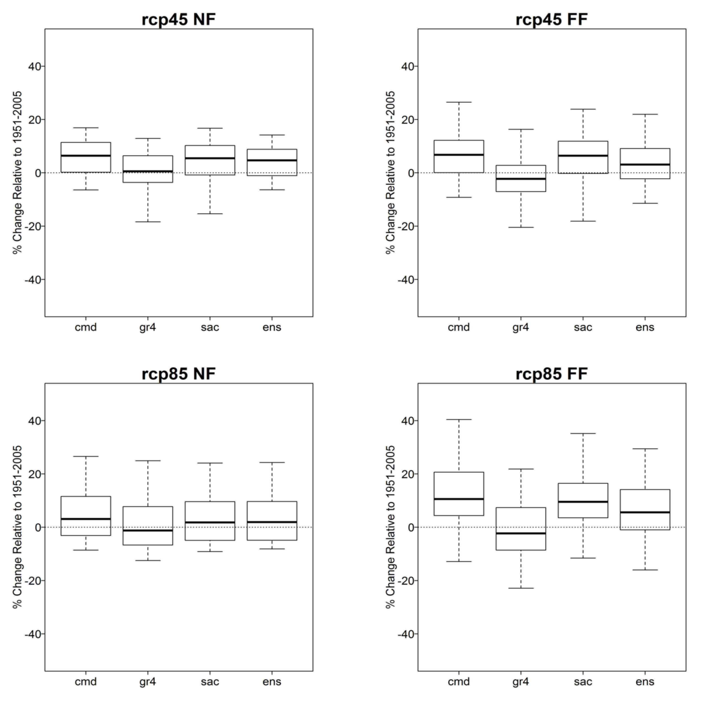
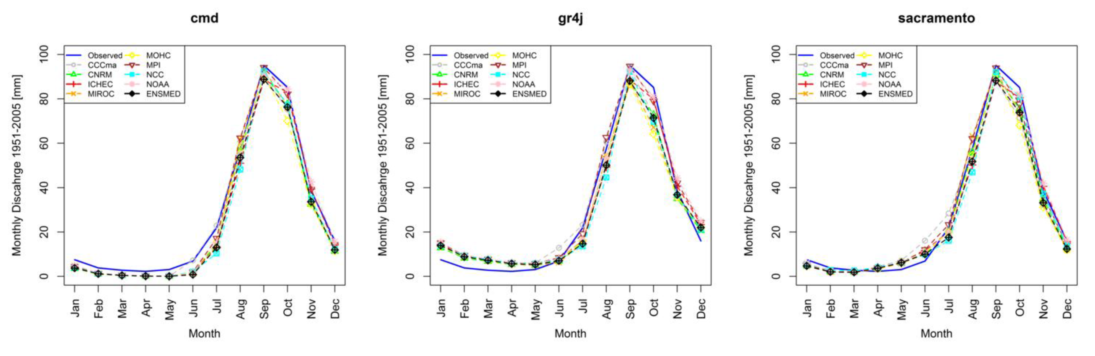
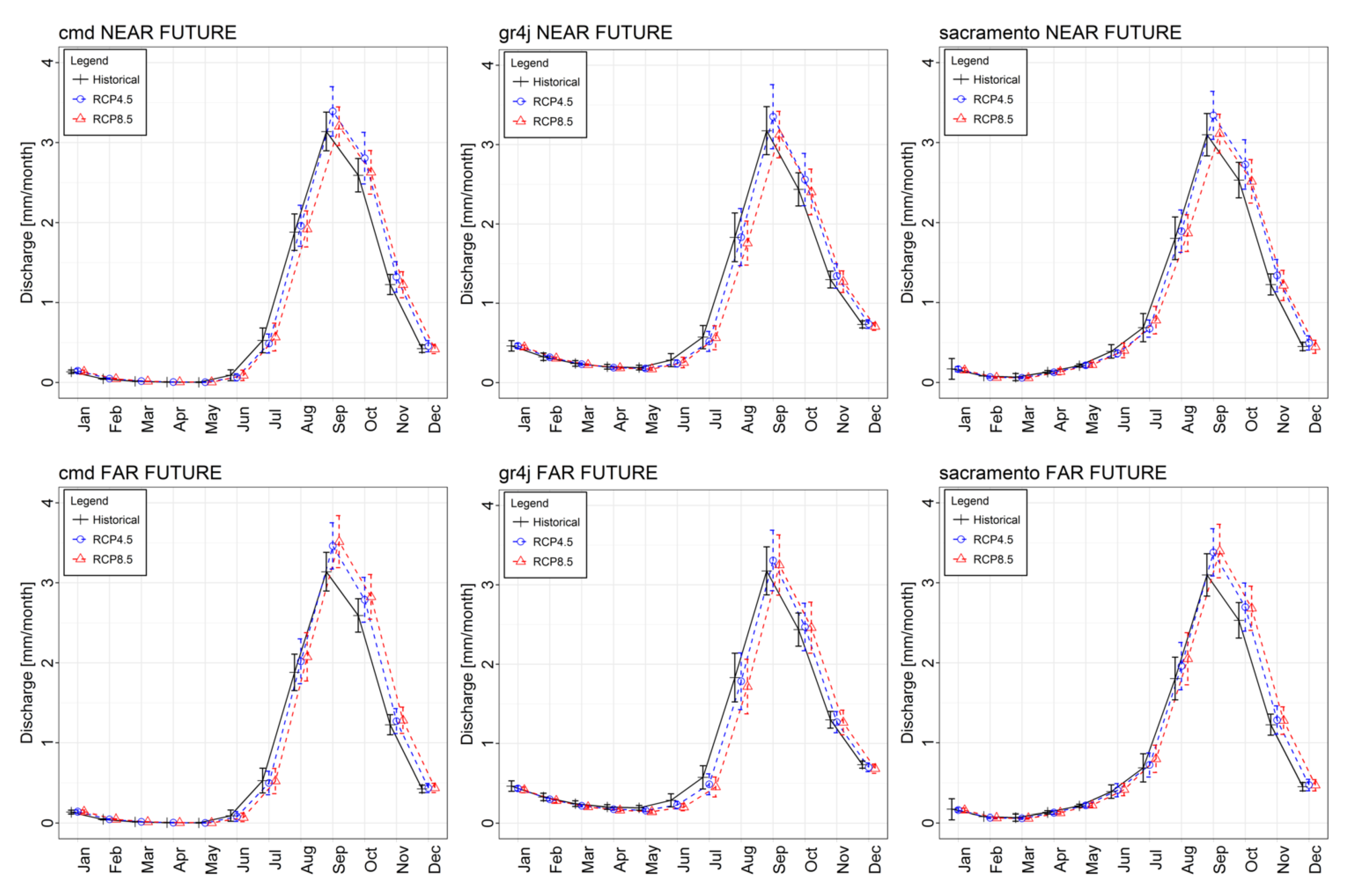
The influence of the model structural uncertainties on the monthly simulated runoff with GCM data is shown in Figure 4 and Figure 5. All the models properly captured the flow patterns from June to December, while only the Sacramento model adequately simulated low flow months (January–May). Figure 5 compares monthly ensemble runoff projections to those of the historical period. Under the RCP4.5 scenario in the near future, the IHACRES-CMD and Sacramento models simulated clear increases in runoff from August to December, while the GR4J model showed that increases will occur from September to November. In the far future (RCP4.5), there will be an increase in runoff from August to November under the simulations of IHACRES-CMD and Sacramento, while GR4J projected runoff decreases in the months of July and August and an increase in September. RCP8.5 runoff projections showed runoff increases from July to October (IHACRES-CMD), the Scaramento model projected increases in July and August, and GR4J simulated decreases from July to December. Far future RCP8.5 simulations experience increases in the months of August to November (IHACRES-CMD) and Scaramento will go through increases from July to November, while the GR4J increase will only occur in September. Annual runoff projections from the three RR models and their ensemble of the hydrological models were aggregated to climatological time-scales and the results are presented in Figure 6. Clear increase in runoff is projected for the IHACRES-CMD and Sacramento models for RCP8.5. The ensemble of the hydrological models was able to amend the effects of uncertain projections made by the GR4J model.
4. Discussion
High efficiency values recorded during the calibration and validation periods indicate the suitability of the three models for runoff simulations in the catchment, particularly with the IHACRES-CMD having the highest NSE, especially during model validation. This is in agreement with the study of Oyerinde et al. [9], who disclosed a similar high efficient runoff simulation with a similar version of the IHACRES—CMD model in the Niger basin. Clear differences in simulated monthly patterns of the different RR models were due to contrasting model structures (structural uncertainties). Structural uncertainties arise from simplified assumptions made in approximating the actual environmental system with mathematical functions [12]. Similar uncertainties in hydrological modelling were reported by Cornelissen et al. [15], where they were ascribed to differences in model parameterization and structure. More robust model parameterisation is responsible for an adequate simulation of low flow by the Sacramento model. The overestimation of low flow by the GR4J model experienced in this study is in line with the work of Demirel et al. [48], who stated that parameter uncertainty has the highest effect on the low flow simulation.
Because the ensemble of the hydrological models is compensating for the effects of model uncertainties, the mean result is a more reliable estimation of future runoff characteristics. The multi-model approach has been proven to be more robust and exhibits a better performance than individual models [49]. Simple multi-model approaches that combine the outputs of hydrological models improve the simulation and forecasting efficiency [49]. This is due to a more accurate representation of the catchment water balance by the hydrological model ensemble [50]. This is in line with the study of Lambert and Boer [51] and Diallo et al. [52], who reported ensembles of models as better predictors than individual models. This finding is also in agreement with Seiller et al. [53], who compared ensembles of twenty hydrological models and concluded that using a single model may provide hazardous results when the model is to be applied in contrasting conditions.
5. Conclusions
The Niger basin was ascribed with high uncertainties in future runoff trends, making hydrological project implementation and evaluation difficult. The potential of using multi climate and multi hydrological models in a robust uncertainty assessment was evaluated in the study. The influence of three (IHACRES-CMD, GR4J, and Sacramento) model structures on the simulated and projected runoff in current and future times was assessed using climate data from eight GCM. The results indicate that multi climate and multi hydrological model simulations help to reduce hydro-climatic modelling uncertainties. Each of the hydrological models was able to properly simulate runoff patterns with high efficiencies in the historical period. The influence of structural uncertainties of the models was prominent in the inability of IHACRES-CMD and GR4J to adequately simulate low flow patterns when compared to observed runoff in the historical period. This led to different trends of projected ensemble (climate models) future runoff by each of the hydrological models. However, these effects were smoothed out in the runoff prediction of the ensemble hydrological and climate models, which is recommended as a better predictor than individual climate and hydrological models.
Acknowledgments
We thank the ESGF, which provided the CORDEX-Africa future climate projections. The Niger Basin Authority is acknowledged for providing the runoff data. We appreciate the R project and the Hydromad group for providing the modelling environments. The Global Precipitation Climatology Project (GPCP) and the Modern Era Retrospective-analysis for Research and Applications (MERRA) are acknowledged for making available their rainfall and temperature datasets. Vincent Olanrewaju Ajayi and Fabien C.C. Hountondji are appreciated for reading through the manuscript.
Author Contributions
The modelling parts and manuscript write-up were done by Oyerinde Ganiyu Titilope and Bernd Diekkrüger.
Conflicts of Interest
The authors declare no conflict of interest.
References
- Druyan, L.M. Studies of 21st-century precipitation trends over West Africa. Int. J. Climatol. 2011, 31, 1415–1424. [Google Scholar] [CrossRef]
- Sylla, M.B.; Giorgi, F.; Coppola, E.; Mariotti, L. Uncertainties in daily rainfall over Africa: Assessment of gridded observation products and evaluation of a regional climate model simulation. Int. J. Climatol. 2013, 33, 1805–1817. [Google Scholar] [CrossRef]
- Ali, A.; Lebel, T. The Sahelian standardized rainfall index revisited. Int. J. Climatol. 2009, 29, 1705–1714. [Google Scholar] [CrossRef]
- Oyerinde, G.T.; Hountondji, F.C.C.; Wisser, D.; Diekkrüger, B.; Lawin, A.E.; Odofin, A.J.; Afouda, A. Hydro-climatic changes in the Niger basin and consistency of local perceptions. Reg. Environ. Chang. 2015, 15, 1627–1637. [Google Scholar] [CrossRef]
- KfW Adaptation to climate change in the upper and middle Niger River Basin. Available online: http://ccsl.iccip.net/niger_river_basin.pdf (accessed on 12 February 2017).
- Mahe, G.; Paturel, J.-E.; Servat, E.; Conway, D.; Dezetter, A. The impact of land use change on soil water holding capacity and river flow modelling in the Nakambe River, Burkina-Faso. J. Hydrol. 2005, 300, 33–43. [Google Scholar] [CrossRef]
- Descroix, L.; Mahé, G.; Lebel, T.; Favreau, G.; Galle, S.; Gautier, E.; Olivry, J.-C.; Albergel, J.; Amogu, O.; Cappelaere, B. Spatio-temporal variability of hydrological regimes around the boundaries between Sahelian and Sudanian areas of West Africa: A synthesis. J. Hydrol. 2009, 375, 90–102. [Google Scholar] [CrossRef]
- Uhlenbrook, S.; Seibert, J.; Leibundgut, C.; Rodhe, A. Prediction uncertainty of conceptual rainfall-runoff models caused by problems in identifying model parameters and structure. Hydrol. Sci. J. 1999, 44, 779–797. [Google Scholar] [CrossRef]
- Oyerinde, G.T.; Wisser, D.; Hountondji, F.C.C.; Odofin, A.J.; Lawin, A.E.; Afouda, A.; Diekkrüger, B. Quantifying Uncertainties in Modeling Climate Change Impacts on Hydropower Production. Climate 2016, 4, 1–15. [Google Scholar] [CrossRef]
- Kay, A.L.; Davies, H.N.; Bell, V.A.; Jones, R.G. Comparison of uncertainty sources for climate change impacts: Flood frequency in England. Clim. Chang. 2009, 92, 41–63. [Google Scholar] [CrossRef] [Green Version]
- Vetter, T.; Huang, S.; Aich, V.; Yang, T.; Wang, X.; Krysanova, V.; Hattermann, F. Multi-model climate impact assessment and intercomparison for three large-scale river. Earth Syst. Dyn. 2015, 6, 17–43. [Google Scholar] [CrossRef]
- Renard, B.; Kavetski, D.; Kuczera, G.; Thyer, M.; Franks, S.W. Understanding predictive uncertainty in hydrologic modeling: The challenge of identifying input and structural errors. Water Resour. Res. 2010, 46, 1–22. [Google Scholar] [CrossRef]
- Knutti, R.; Sedláč, J. Robustness and uncertainties in the new CMIP5 climate model projections. Nat. Clim. Chang. 2013, 3, 369–373. [Google Scholar] [CrossRef]
- Giorgi, F.; Francisco, R. Evaluating uncertainties in the prediction of regional climate change. Geophys. Res. Lett. 2000, 27, 1295–1298. [Google Scholar] [CrossRef]
- Cornelissen, T.; Diekkrüger, B.; Giertz, S. A comparison of hydrological models for assessing the impact of land use and climate change on discharge in a tropical catchment. J. Hydrol. 2013, 498, 221–236. [Google Scholar] [CrossRef]
- Yira, Y.; Diekkrüger, B.; Steup, G.; Bossa, A.Y. Impact of climate change on hydrological conditions in a tropical West African catchment using an ensemble of climate simulations. Hydrol. Earth Syst. Sci. 2017, 21, 2143–2161. [Google Scholar] [CrossRef]
- Ogilvie, A.; Mahéé, G.; Ward, J.; Serpantiéé, G.; Lemoalle, J.; Morand, P.; Barbier, B.; Kaczan, D.; Lukasiewicz, A.; Paturel, J.; et al. Water, agriculture and poverty in the Niger River basin. Water Int. 2010, 35, 594–622. [Google Scholar] [CrossRef]
- Andrews, F.T.; Croke, B.F.W.; Jakeman, A.J. An open software environment for hydrological model assessment and development. Environ. Model. Softw. 2011, 26, 1171–1185. [Google Scholar] [CrossRef]
- Croke, B.F.W.; Jakeman, A.J. A catchment moisture deficit module for the IHACRES rainfall-runoff model. Environ. Model. Softw. 2004, 19, 1–5. [Google Scholar] [CrossRef]
- Burnash, R.J. The NWS River Forecast System—Catchment Modeling. In Computer Models of Watershed Hydrology; Singh, V.P., Ed.; Water Resource Publications: Littleton, CO, USA, 2012; p. 1144. [Google Scholar]
- Perrin, C.; Michel, C.; Andréassian, V. Improvement of a parsimonious model for streamflow simulation. J. Hydrol. 2003, 279, 275–289. [Google Scholar] [CrossRef]
- Oyerinde, G.T.; Fademi, I.O.; Denton, O.A. Modeling runoff with satellite-based rainfall estimates in the Niger basin. Cogent Food Agric. 2017, 3, 1–23. [Google Scholar] [CrossRef]
- Oyerinde, G.; Hountondji, F.C.C.; Lawin, A.E.; Odofin, A.J.; Afouda, A.; Diekkrüger, B. Improving Hydro-Climatic Projections with Bias-Correction in Sahelian Niger Basin, West Africa. Climate 2017, 5, 1–18. [Google Scholar] [CrossRef]
- Gosset, M.; Viarre, J. Evaluation of several rainfall products used for hydrological applications over West Africa using two high-resolution gauge networks. Q. J. R. Meteorol. Soc. 2013, 139, 923–940. [Google Scholar] [CrossRef]
- Nash, J.E.; Sutcliffe, J.V. River flow forecasting through conceptual models part I—A discussion of principles. J. Hydrol. 1970, 10, 282–290. [Google Scholar] [CrossRef]
- Zambrano-Bigiarini, M. Graphical Goodness of Fit Description. Available online: https://www.rforge.net/doc/packages/hydroGOF/ggof.html (accessed on 17 May 2017).
- Moriasi, D.N.; Arnold, J.G.; van Liew, M.W.; Bingner, R.L.; Harmel, R.D.; Veith, T.L. Veith Model Evaluation Guidelines for Systematic Quantification of Accuracy in Watershed Simulations. Trans. ASABE 2007, 50, 885–900. [Google Scholar] [CrossRef]
- Criss, R.E.; Winston, W.E. Do Nash values have value? Discussion and alternate proposals. Hydrol. Process. 2008, 22, 2723–2725. [Google Scholar] [CrossRef]
- Kling, H.; Fuchs, M.; Paulin, M. Runoff conditions in the upper Danube basin under an ensemble of climate change scenarios. J. Hydrol. 2012, 424–425, 264–277. [Google Scholar] [CrossRef]
- Gupta, H.V.; Kling, H.; Yilmaz, K.K.; Martinez, G.F. Decomposition of the mean squared error and NSE performance criteria: Implications for improving hydrological modelling. J. Hydrol. 2009, 377, 80–91. [Google Scholar] [CrossRef]
- Beven, K.; Binley, A. The future of distributed models: Model calibration and uncertainty prediction. Hydrol. Process. 1992, 6, 279–298. [Google Scholar] [CrossRef]
- Chaibou Begou, J.; Jomaa, S.; Benabdallah, S.; Bazie, P.; Afouda, A.; Rode, M. Multi-Site Validation of the SWAT Model on the Bani Catchment: Model Performance and Predictive Uncertainty. Water 2016, 8, 178. [Google Scholar] [CrossRef]
- Abbaspour, K.C.; Johnson, C.A.; van Genuchten, M.T. Estimating Uncertain Flow and Transport Parameters Using a Sequential Uncertainty Fitting Procedure. Vad. Zone J. 2004, 3, 1340. [Google Scholar] [CrossRef]
- Soetaert, K.; Petzoldt, T. Inverse Modelling, Sensitivity and Monte Carlo Analysis in R Using Package FME. J. Stat. Softw. 2010, 33, 1–28. [Google Scholar] [CrossRef]
- Huffman, G.J.; Adler, R.F.; Arkin, P.; Chang, A.; Ferraro, R.; Gruber, A.; Janowiak, J.; Mcnab, A.; Rudolf, B.; Schneider, U. The Global Precipitation Climatology Project ( GPCP ) Combined Precipitation Dataset. Bull. Am. Meteorol. Soc. 1997, 78, 5–20. [Google Scholar] [CrossRef]
- Rienecker, M.M.; Suarez, M.J.; Gelaro, R.; Todling, R.; Bacmeister, J.; Liu, E.; Bosilovich, M.G.; Schubert, S.D.; Takacs, L.; Kim, G.-K.; et al. MERRA: NASA’s Modern-Era Retrospective Analysis for Research and Applications. J. Clim. 2011, 24, 3624–3648. [Google Scholar] [CrossRef]
- Oudin, L.; Hervieu, F.; Michel, C.; Perrin, C.; Andréassian, V.; Anctil, F.; Loumagne, C. Which potential evapotranspiration input for a lumped rainfall–runoff model? J. Hydrol. 2005, 303, 290–306. [Google Scholar] [CrossRef]
- Lehner, B.; Verdin, K.; Jarvis, A. New global hydrography derived from spaceborne elevation data. EOS Trans. Am. Geophys. Union 2008, 89, 93–94. [Google Scholar] [CrossRef]
- Jasiewicz, J.; Metz, M. A new GRASS GIS toolkit for Hortonian analysis of drainage networks. Comput. Geosci. 2011, 37, 1162–1173. [Google Scholar] [CrossRef]
- Lucio, P.; Molion, L.; Valadão, C.; Conde, F.; Ramos, A.; MLD, M. Dynamical outlines of the rainfall variability and the ITCZ role over the West Sahel. Atmos. Clim. Sci. 2012, 2, 337–350. [Google Scholar] [CrossRef]
- Taylor, K.E.; Stouffer, R.J.; Meehl, G.A. An Overview of CMIP5 and the Experiment Design. Bull. Am. Meteorol. Soc. 2012, 93, 485–498. [Google Scholar] [CrossRef]
- Giorgi, F.; Jones, C.; Asrar, G.R. Addressing climate information needs at the regional level: The CORDEX framework. WMO Bull. 2009, 58, 175–183. [Google Scholar]
- Mounkaila, M.S.; Abiodun, B.J.; Bayo Omotosho, J. Assessing the capability of CORDEX models in simulating onset of rainfall in West Africa. Theor. Appl. Climatol. 2014. [Google Scholar] [CrossRef]
- Tall, M.; Sylla, M.B.; Diallo, I.; Pal, J.S.; Faye, A.; Mbaye, M.L.; Gaye, A.T. Projected impact of climate change in the hydroclimatology of Senegal with a focus over the Lake of Guiers for the twenty-first century. Theor. Appl. Climatol. 2016, 1–11. [Google Scholar] [CrossRef]
- Ravazzani, G.; Dalla Valle, F.; Gaudard, L.; Mendlik, T.; Gobiet, A.; Mancini, M. Assessing Climate Impacts on Hydropower Production: The Case of the Toce River Basin. Climate 2016, 4, 16. [Google Scholar] [CrossRef] [Green Version]
- Maraun, D. Bias Correction, Quantile Mapping, and Downscaling: Revisiting the Inflation Issue. J. Clim. 2013, 26, 2137–2143. [Google Scholar] [CrossRef] [Green Version]
- Su, F.; Duan, X.; Chen, D.; Hao, Z.; Cuo, L. Evaluation of the Global Climate Models in the CMIP5 over the Tibetan Plateau. J. Clim. 2013, 26, 3187–3208. [Google Scholar] [CrossRef]
- Demirel, M.C.; Booij, M.J.; Hoekstra, A.Y. Effect of different uncertainty sources on the skill of 10 day ensemble low flow forecasts for two hydrological models. Water Resour. Res. 2013, 49, 4035–4053. [Google Scholar] [CrossRef]
- Nicolle, P.; Pushpalatha, R.; Perrin, C.; François, D.; Thiéry, D.; Mathevet, T.; Le Lay, M.; Besson, F.; Soubeyroux, J.M.; Viel, C.; et al. Benchmarking hydrological models for low-flow simulation and forecasting on French catchments. Hydrol. Earth Syst. Sci. 2014, 18, 2829–2857. [Google Scholar] [CrossRef] [Green Version]
- Thapa, B.R.; Ishidaira, H.; Pandey, V.P.; Shakya, N.M. A multi-model approach for analyzing water balance dynamics in Kathmandu Valley, Nepal. J. Hydrol. Reg. Stud. 2017, 9, 149–162. [Google Scholar] [CrossRef]
- Lambert, S.J.; Boer, G.J. CMIP1 evaluation and intercomparison of coupled climate models. Clim. Dyn. 2001, 17, 83–106. [Google Scholar] [CrossRef]
- Diallo, I.; Sylla, M.B.; Giorgi, F.; Gaye, A.T.; Camara, M. Multimodel GCM-RCM Ensemble-Based Projections of Temperature and Precipitation over West Africa for the Early 21st Century. Int. J. Geophys. 2012, 2012, 1–19. [Google Scholar] [CrossRef]
- Seiller, G.; Anctil, F.; Perrin, C. Multimodel evaluation of twenty lumped hydrological models under contrasted climate conditions. Hydrol. Earth Syst. Sci. 2012, 16, 1171–1189. [Google Scholar] [CrossRef]
Figure 1.
Location of the Koulikoro catchment in the Niger basin.
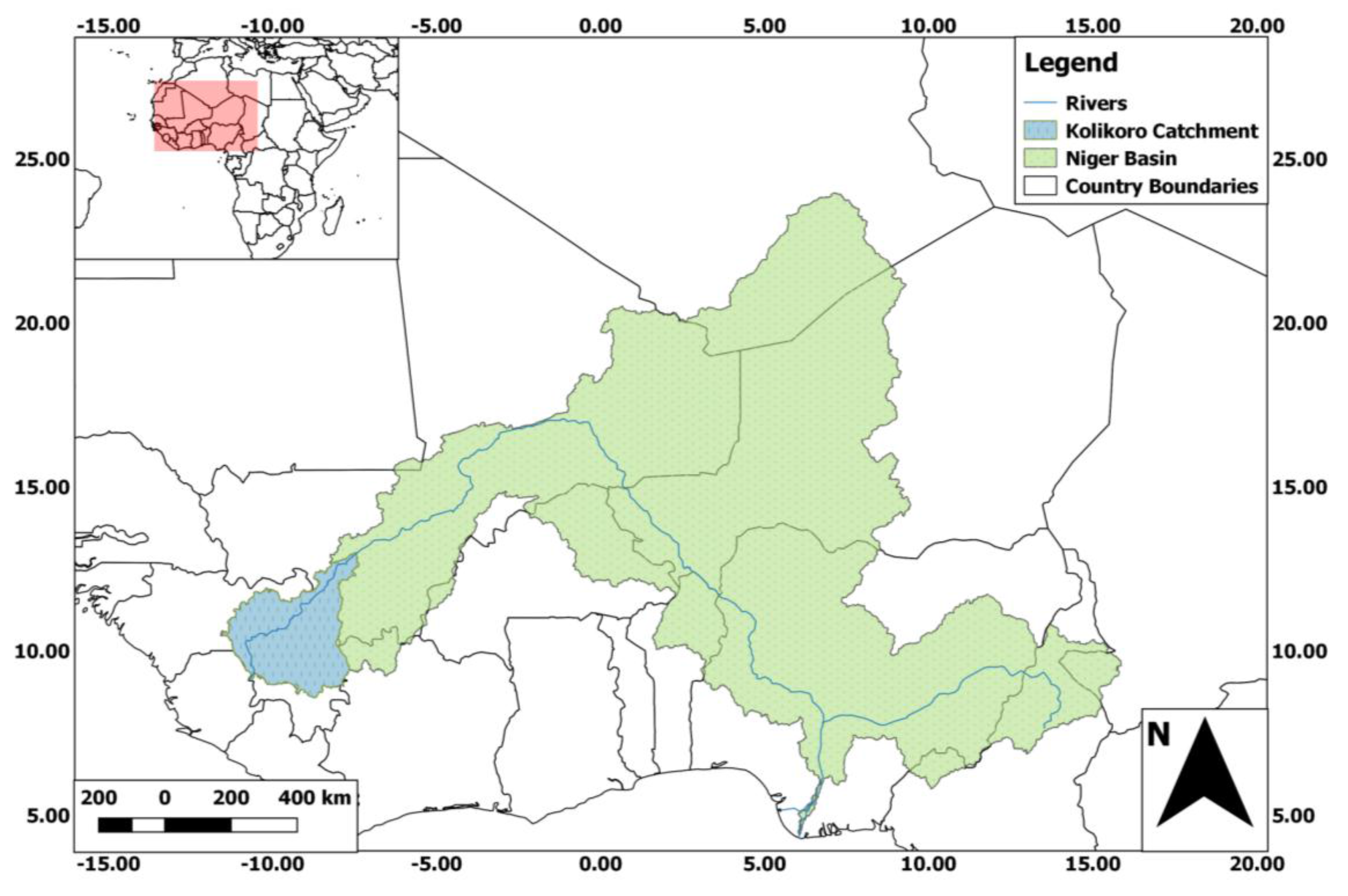
Figure 2.
Generalized Likelihood Uncertainty Estimation (GLUE) ensemble median and uncertainty bands from behavioural parameters of 10,000 parameter sets during the calibration (1997–2003) and validation (2004–2010) periods.
Figure 2.
Generalized Likelihood Uncertainty Estimation (GLUE) ensemble median and uncertainty bands from behavioural parameters of 10,000 parameter sets during the calibration (1997–2003) and validation (2004–2010) periods.
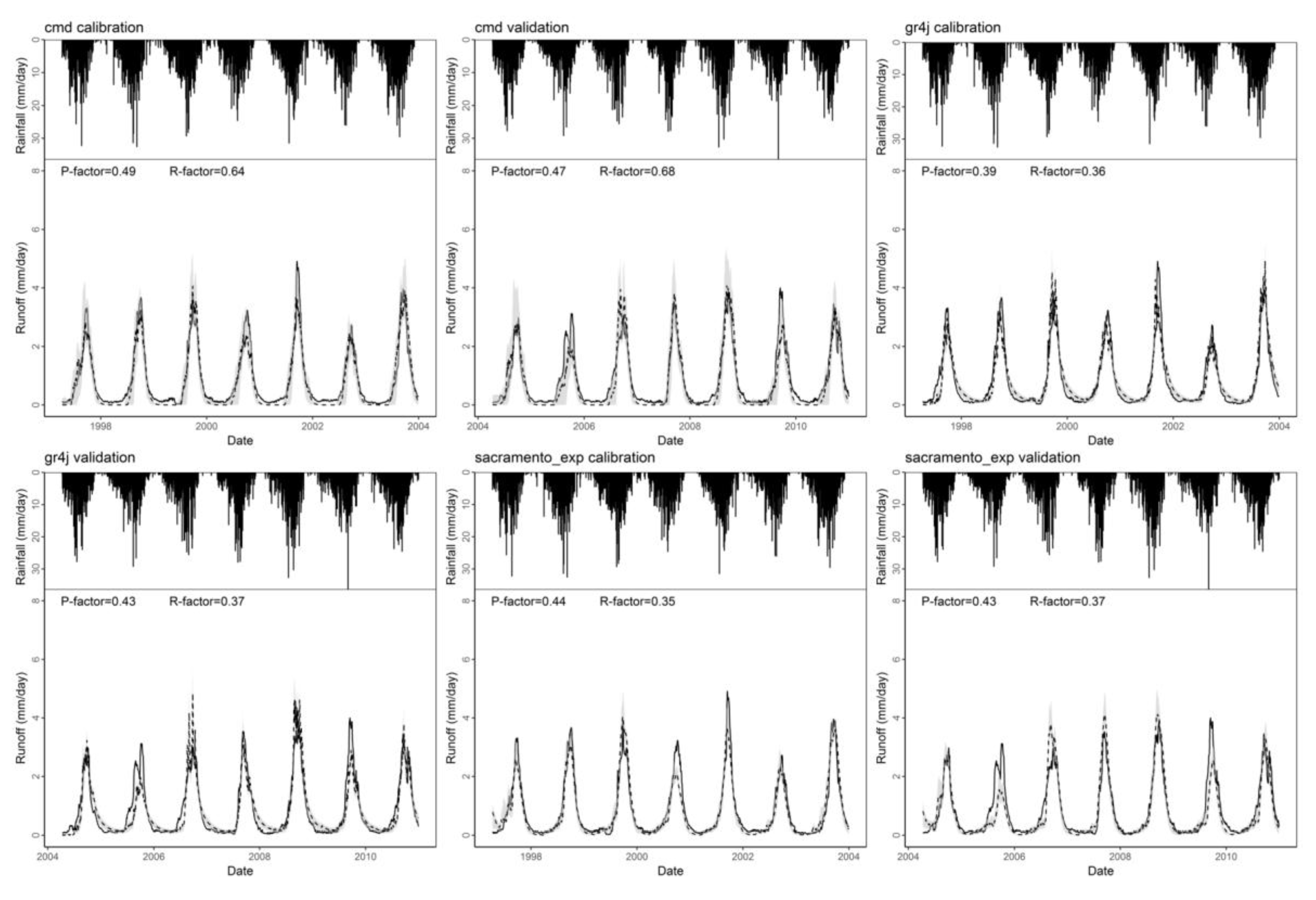
Figure 3.
Sensitivity of simulated runoff from 10,000 parameter sets for three RR models and their most sensitive model parameter.
Figure 3.
Sensitivity of simulated runoff from 10,000 parameter sets for three RR models and their most sensitive model parameter.
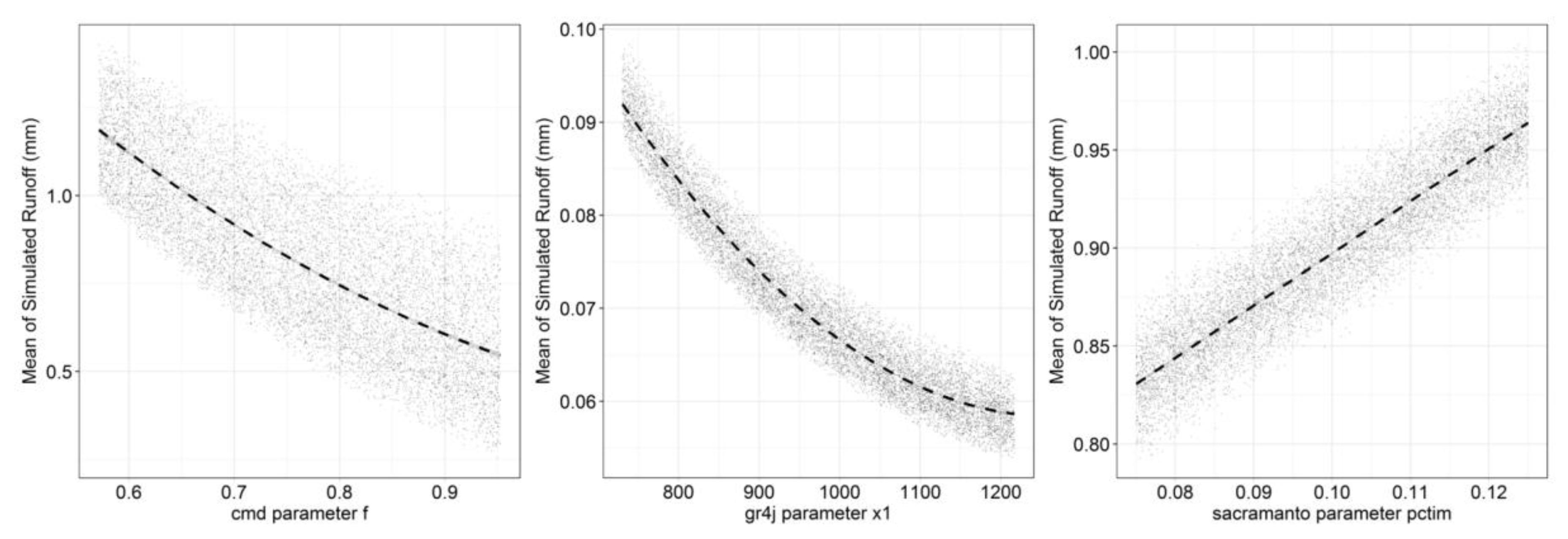
Figure 4.
Comparison of historical (1951–2005) mean monthly discharge from eight GCMs and ensemble with the observed discharge for IHACRES-CMD (cmd), GR4J (gr4j) and Sacramento models .
Figure 4.
Comparison of historical (1951–2005) mean monthly discharge from eight GCMs and ensemble with the observed discharge for IHACRES-CMD (cmd), GR4J (gr4j) and Sacramento models .

Figure 5.
Effect of model structure uncertainty on ensemble simulated mean monthly discharge from eight GCMs in the past (1951–2005), as well as the near (2010–2035) and far (2036–2099) future.
Figure 5.
Effect of model structure uncertainty on ensemble simulated mean monthly discharge from eight GCMs in the past (1951–2005), as well as the near (2010–2035) and far (2036–2099) future.

Figure 6.
Effect of model structure uncertainty on climatological trends of the ensemble mean projected runoff at the Near Future (NF: 2010–2035) and Far Future (FF: 2036–2099).
Figure 6.
Effect of model structure uncertainty on climatological trends of the ensemble mean projected runoff at the Near Future (NF: 2010–2035) and Far Future (FF: 2036–2099).

Table 1.
Parameter descriptions and correlation coefficients (r) with simulated runoff from 10,000 model runs.
Table 1.
Parameter descriptions and correlation coefficients (r) with simulated runoff from 10,000 model runs.
| Parameter | Description | Range | Calibrated Value | r Values between Mean Simulated Runoff and Parameters | |
|---|---|---|---|---|---|
| IHACRES-CMD | |||||
| f | Plant stress threshold as a proportion of d. | 0.01–3 | 0.723 | −0.791 | |
| e | Temperature to PET conversion factor. | 0.01–1.5 | 0.795 | −0.587 | |
| d | Threshold for producing flow. | 50–550 | 402.798 | −0.171 | |
| GR4J | |||||
| x1 | maximum capacity of the production store (mm). | 100–1200 | 891.941 | −0.950 | |
| x2 | groundwater exchange coefficient (mm). | −5–+3 | −0.564 | 0.129 | |
| x3 | one day ahead maximum capacity of the routing store (mm). | 20–300 | 214.509 | −0.209 | |
| x4 | time base of unit hydrograph (time steps). | 1.1–2.9 | 2.807 | −0.007 | |
| Sacramento | |||||
| uztwm | Upper zone tension water maximum capacity (mm). | 1–150 | 75.367 | −0.173 | |
| uzfwm | Upper zone free water maximum capacity (mm). | 1–150 | 82.171 | 0.015 | |
| uzk | Lateral drainage rate of upper zone free water expressed as a fraction of contents per day. | 0.5–1 | 0.207 | 0.019 | |
| pctim | The fraction of the catchment which produces impervious runoff during low flow conditions. | 0.1–1 | 0.073 | 0.918 | |
| adimp | The additional fraction of the catchment which exhibits impervious characteristics when the catchment’s tension water requirements are met. | 0–0.4 | 0.002 | −0.031 | |
| zperc | Maximum percolation (from upper zone free water into the lower zone) rate coefficient. | 1–250 | 70.797 | 0.003 | |
| rexp | An exponent determining the rate of change of the percolation rate with changing lower zone water contents. | 0–5 | 4.700 | 0.005 | |
| lztwm | Lower zone tension water maximum capacity (mm). | 1–500 | 10.424 | −0.336 | |
| lzfsm | Lower zone supplemental free water maximum capacity (mm). | 1–1000 | 251.439 | 0.103 | |
| lzfpm | Lower zone primary free water maximum capacity (mm). | 1–1000 | 576.492 | 0.091 | |
| lzsk | Lateral drainage rate of lower zone supplemental free water expressed as a fraction of contents per day. | 0.02–0.25 | 0.155 | 0.007 | |
| lzpk | Lateral drainage rate of lower zone primary free water expressed as a fraction of contents per day. | 0.0004–0.25 | 0.038 | 0.005 | |
| pfree | Direct percolation fraction from upper to lower zone free water. | 0–0.6 | 0.017 | 0.025 | |
Table 2.
List of CMIP5 GCM models considered in the study.
| Modelling Center (or Group) | Institute ID | Model Name |
|---|---|---|
| Canadian Centre for Climate Modelling and Analysis | CCCMA | CanESM2 |
| Centre National de Recherches Météorologiques/Centre Européen de Recherche et Formation Avancée en Calcul Scientifique | CNRM-CERFACS | CNRM-CM5 |
| NOAA Geophysical Fluid Dynamics Laboratory | NOAA GFDL | GFDL-ESM2M |
| Met Office Hadley Centre (additional HadGEM2-ES realizations contributed by Instituto Nacional de Pesquisas Espaciais) | MOHC | HadGEM2-ES |
| Atmosphere and Ocean Research Institute (The University of Tokyo), National Institute for Environmental Studies, and Japan Agency for Marine-Earth Science and Technology | MIROC | MIROC5 |
| Max-Planck-Institut für Meteorologie (Max Planck Institute for Meteorology) | MPI-M | MPI-ESM-LR |
| Norwegian Climate Centre | NCC | NorESM1-M |
| EC-EARTH consortium | ICHEC | EC-EARTH |
Table 3.
Comparative efficiencies of three hydrological models (IHACRES Catchment Moisture Deficit—CMD, GR4J and Sacramento).
Table 3.
Comparative efficiencies of three hydrological models (IHACRES Catchment Moisture Deficit—CMD, GR4J and Sacramento).
| Models | ME | RMSE | RSD | NSE | KGE | VE |
|---|---|---|---|---|---|---|
| Calibration (1997–2003) | ||||||
| Sacramento | −0.07 | 0.31 | 0.93 | 0.91 | 0.89 | 0.77 |
| GR4J | 0.01 | 0.36 | 0.92 | 0.88 | 0.90 | 0.72 |
| IHACRES-CMD | −0.10 | 0.30 | 0.99 | 0.92 | 0.88 | 0.75 |
| Validation (2004–2010) | ||||||
| Sacramento | −0.06 | 0.43 | 1.02 | 0.81 | 0.88 | 0.7 |
| GR4J | −0.02 | 0.39 | 0.95 | 0.84 | 0.9 | 0.69 |
| IHACRES-CMD | −0.12 | 0.37 | 1.05 | 0.86 | 0.84 | 0.71 |
© 2017 by the authors. Licensee MDPI, Basel, Switzerland. This article is an open access article distributed under the terms and conditions of the Creative Commons Attribution (CC BY) license (http://creativecommons.org/licenses/by/4.0/).
Share and Cite
MDPI and ACS Style
Oyerinde, G.T.; Diekkrüger, B. Influence of Parameter Sensitivity and Uncertainty on Projected Runoff in the Upper Niger Basin under a Changing Climate. Climate 2017, 5, 67. https://doi.org/10.3390/cli5030067
AMA Style
Oyerinde GT, Diekkrüger B. Influence of Parameter Sensitivity and Uncertainty on Projected Runoff in the Upper Niger Basin under a Changing Climate. Climate. 2017; 5(3):67. https://doi.org/10.3390/cli5030067
Chicago/Turabian StyleOyerinde, Ganiyu Titilope, and Bernd Diekkrüger. 2017. "Influence of Parameter Sensitivity and Uncertainty on Projected Runoff in the Upper Niger Basin under a Changing Climate" Climate 5, no. 3: 67. https://doi.org/10.3390/cli5030067
Note that from the first issue of 2016, this journal uses article numbers instead of page numbers. See further details here.