
Rainfall Variability in January in the Federal District of Brazil from 1981 to 2010


1
Departament of Geography of University of Brasília, Brasília 70910-900, Brazil
2
Brazilian Agricultural Research Corporation, Brasília 70770-901, Brazil
*
Author to whom correspondence should be addressed.
Climate 2017, 5(3), 68; https://doi.org/10.3390/cli5030068
Submission received: 25 July 2017
/
Revised: 18 August 2017
/
Accepted: 22 August 2017
/
Published: 28 August 2017
(This article belongs to the Special Issue Studies and Perspectives of Climatology in Brazil)
Abstract
:The Federal District is a politically and economically important part of Brazil, which suffers from water stress. Exploratory analyzes were conducted using data on rainfall in the Federal District from the monthly precipitation time series to assess the rainfall variability in January, a month that falls in the middle of the rainy season in the region. A time series of 30 years (1981–2010), recorded at 19 rain gauges was analyzed. The resulting exploratory analyses show a gradient of increasing rainfall in the westward direction in the Federal District. Moreover, the time series shows a moderate inter-annual variability in rainfall volume, which is, however, of a stationary nature.
1. Introduction
Water is one of the most important natural resources as it is essential for assuring the quality of life and social and economic development of populations, while also constituting a component of the landscape and the environment, Andrade et al. [1]. In the global geopolitical scenario, water has always been prioritized by societies, especially those that experience constant water shortages.
This is why any action designed to assist the management of water resources is so important in the broader context of local, regional, and national government policies. Any actions that can improve our understanding of the hydrologic cycle will always be useful for water resource management. As Andrade et al. [1] note, “it is therefore fundamental to think strategically about this asset [water], about how to manage it, and to make policies for its conservation, in view of the fact that the world’s fresh water will certainly be in short supply”.
The most important method by which water is transported across geographic space is precipitation in the form of rain, whose measurement, by whatever scale, can help us better understand the water cycle.
The Federal District is a politically and economically important part of Brazil. It is situated in the central region of the country and covers an area of 5799.999 km2, according to IBGE resolution #1 passed on 15 January 2013, published in the official government gazette, Diário Oficial da União, on 23 January 2013.
According to Setti et al. [2], five Brazilian states and the Federal District “have water availability of between 1000 m3/inhabitant/year and 1700 m3/inhabitant/year, which constitutes a situation of periodic and regular water stress.” In the Federal District, the per capita water availability is 1537 m3/inhabitant/year [3], and “47% of annual precipitation falls between December and March” [4]. These data are consistent with the monthly accumulated precipitation recorded in the Climate Normals of Brazil from 1961 to 1990, from the Brasília weather station, as shown in Figure 1.
In the literature, there are some studies that have directly addressed the issue of rainfall in the Federal District. Anunciação [6] used techniques based on neural networks to classify the summer there into six weather regimes, two with a higher precipitation rate, when the prevailing winds are from the northwest, and two with a lower rate, when the prevailing winds are from the southeast.
Steinke, et al. [7] made a preliminary analysis of the beginning and end of the rainy season in the Federal District in order to obtain a better understanding of its climate. Their findings show that there is irregular rainfall between late September and early November, and between early April and early May, the transition periods between the rainy and dry seasons. Meanwhile, Reinke et al. [8] analyzed the beginning and the end of the rainy season in Brasília (Brasília weather station) using high-frequency data obtained from daily-accumulated rainfall at the INMET (Instituto Nacional de Meteorologia) station. They found that aside from the regular summer rains, there is also precipitation during the transition periods from the dry to rainy season and from the rainy to dry season.
The aim of this study is to make exploratory analyses using rainfall data for the Federal District from the monthly rainfall time series to assess rainfall variability in the month of January, which is a typical month from the rainy season in the region.
2. Materials and Methods
2.1. Rainfall Data
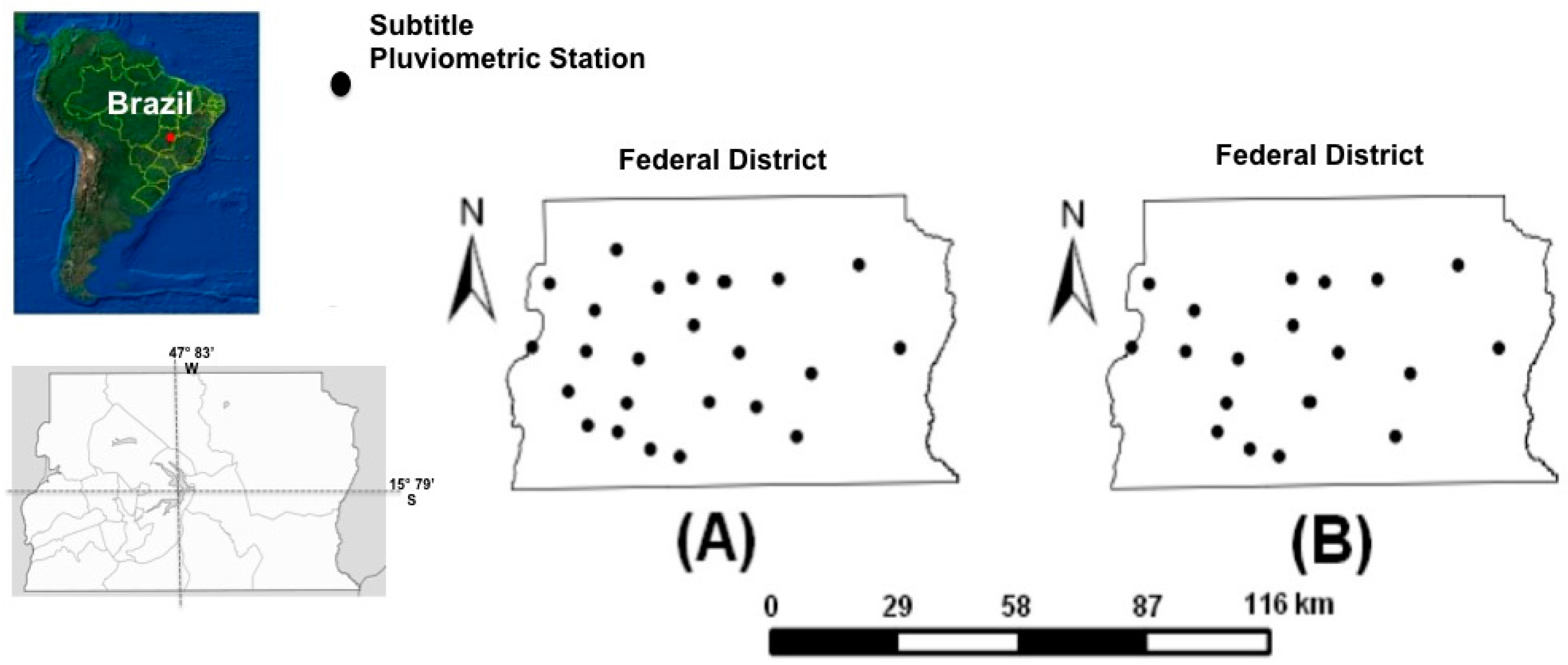
In this study, daily rainfall data from 27 rain gauges maintained by the Brasilia water utility, Companhia de Águas e Esgotos de Brasília (CAESB), were used (see Figure 2A). For each of these gauges, the total monthly-accumulated rainfall in the twelve months of the year from 1971 to 2010 was calculated—the period for which daily rainfall data are available. Only the data for January were considered because this month is statistically considered the rainiest within the rainy season in the Federal District.
However, not all of the 27 gauges had rainfall data for every month in this four-decade-long period. Some only had more recent data (e.g., from 2007 to 2009), while others had no data from most of the 1970s (only beginning in 1978), and still others had some random gaps in their data for days or even months. In view of these limitations, it was decided to only draw on data from 1981 to 2010, for which most of the gauges had data, albeit with some gaps. Nineteen of the 27 gauges (see Figure 2A) had complete or almost complete data, and were therefore chosen to be considered in this study. Their geographic location is shown in Figure 2B.
As already mentioned, the 19 gauges in Figure 2B did have some gaps in their daily records, so an interpolation procedure was carried out based on the regional weighting method [9]. Only a few months were adjusted: of the 570 months of January considered (30 from each of the 19 gauges), just 12 had to have their data interpolated. The other 558 months considered did not need the original CAESB data adjusted at all.
The Federal District, is located in the region of Central Brazil, with relief inserted in the morphoscultural composition defined as Central Plateau, region characterized by surfaces of old planes. The main geomorphological fact of the Federal District is the connection of two large hydrographic basins of Brazil, through the amended waters, a path that drains to the North and South, forming the sources of the Tocantins-Araguaia Hydrographic Basin to the North and the Hydrographic Basin the Prata River to the South. The altitudes in the Federal District vary from 720 to 1340 m, and the highest regions are located in the west, as shown in Figure 3.
2.2. Spatial Representativeness of the 19 Rain Gauges
After selecting the 19 gauges and executing the interpolation procedure, an analysis was conducted to ascertain whether the spatial position of the stations was in fact representative of the geographic space of the Federal District. First, QGIS 2.0 (Quantum GIS) software was used to calculate the approximate area where each of the 19 gauges is situated (Figure 4).
As shown in Figure 4A, the approximate area of the Federal District as calculated using QGIS 2.0 was 5703 km2, an area very similar to its official size (5799.999 km2). Figure 4B shows that the hatched area, representing the space covered by the 19 gauges occupies approximately 3554 km2, corresponding to around 61% of the geographic area of the Federal District, which in principle indicates that the 19 gauges combined provide reasonable coverage of its territory, although there is a greater concentration of these in the western part of the territory.
In studies analyzing the spatial patterns of individual events, the idea is essentially to identify whether the events of interest occur in a clustered, dispersed, or random manner in the study area. An assessment of the distribution of the CAESB gauges in the Federal District was therefore carried out. It was hoped that their distribution pattern would be predominantly dispersed, because this would indicate that the records collected at these points would be more representative of the Federal District as a whole. Taylor (1977) presents the R scale this way:
“Let’s assume that we have measured the distance r between every point in a given pattern and its nearest neighbor. If we take the average of all these distances, we produce a value ra.(…) We know from our previous discussion that a random process is associated with the Poisson probability functions. We can use this distribution to derive expected average nearest neighbor distances for a randomly generated pattern. It is known that this expected average distance for a randomness assumption is given by re = 1/(2*root (n/A)) where n is the number of points and A is the area of the study region.” (TAYLOR, 1977, p. 136, 137)
Essentially, the R scale is a “divergence” of the actual point pattern (measured by ra) ratio from randomness (measured by re) given by R = ra/re.
A k-nearest neighbors analysis was conducted for this purpose, based on the R scale. According to Taylor (1977), 0 ≤ R ≤ 2.149. R-values near 1 indicate a distribution pattern that is random. R-values below 1 represent an increasingly clustered pattern of distribution, such that R = 0 indicates maximum clustering, when all the events take place at the same point in the space under study. Finally, R-values over 1 indicate an increasing pattern of dispersion.
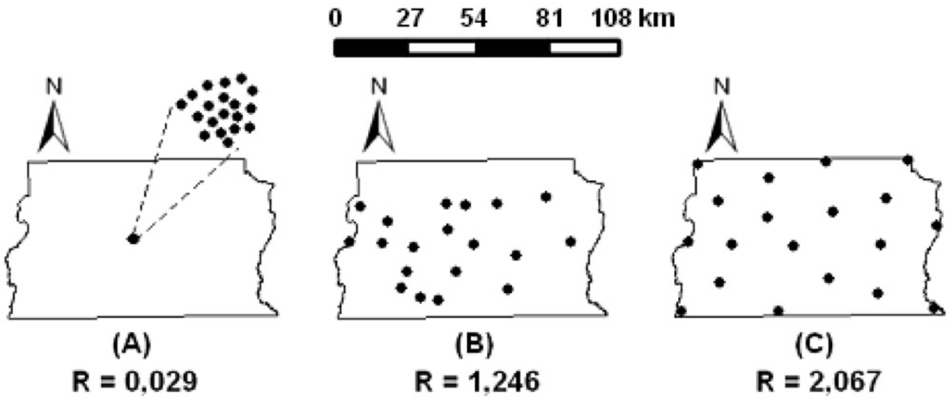
When the R value for the distribution pattern of the points representing the 19 rain gauges was calculated, it was found that R = 1.246. Although the number of elements in the sample is small (just 19 observations), conducting a statistical hypothesis test, where H0 = “the spatial distribution pattern of the 19 observations is random (i.e., R = 1)” and H1 = “the spatial distribution pattern of the 19 observations is not random (i.e., either it is clustered or it is dispersed: R ≠ 1)”, a z-score of 2.047738 and a p-value of 0.040578 were obtained.
For the purposes of a visual comparison, Figure 5 shows three spatial arrangements of the 19 rain gauges in the Federal District. The first one represents a hypothetical situation whereby the 19 gauges are very close to one another, which would be a clustered pattern. The second corresponds to the real location of the 19 gauges, as presented in Figure 2B. The third is another hypothetical situation, this time where the 19 rain gauges would be strongly dispersed.
The point pattern shown in Figure 5C would be the ideal situation of representativeness for the scope of this study. The R value of 1.246 for the real distribution of the 19 rainfall stations in the Federal District, as shown in Figure 5B, could indicate a tendency towards a more random distribution. However, one could also say that there is a slight tendency for the patterns to be dispersed, with a slight tendency towards repulsion. According to the results of the hypothesis test, this is significant to the level of α = 4.0578%, which means the null hypothesis (H0) is rejected in favor of H1.
It would certainly not be true to say that the dispersion pattern is clustered. This therefore makes the hypothesis that the 19 gauges fairly represent the volume of rainfall across the whole geographic space of the Federal District plausible in view of the fact that they are relatively well spatially dispersed. In other words, according to the analysis made, it is fair to take the rainfall measured at the 19 rain gauges as representative of the rainfall in the whole of the Federal District.
3. Results
3.1. Descriptive Statistics of Rainfall Distribution at the 19 Rain Gauges
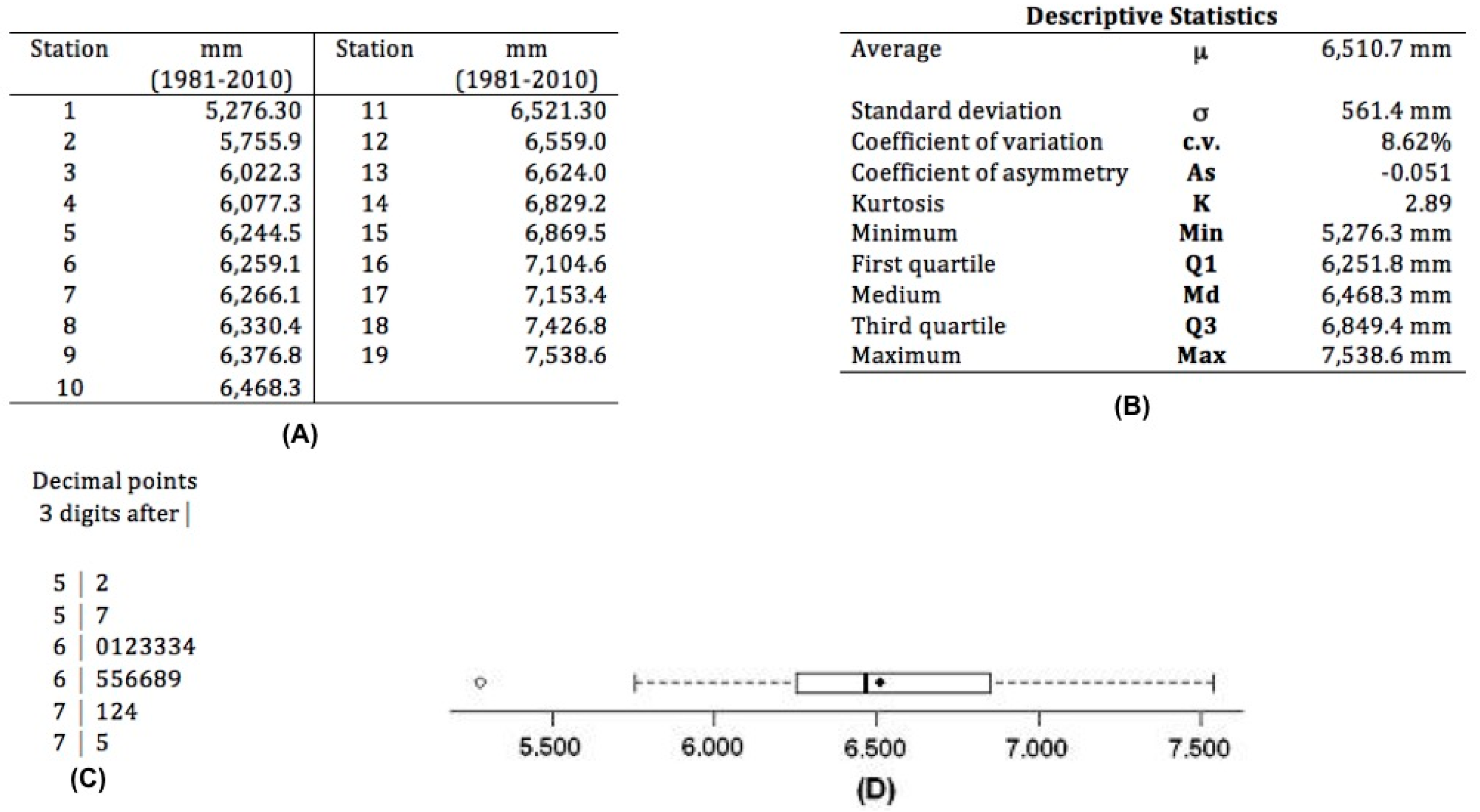
Having ascertained that the 19 rain gauges adequately represent the rainfall in the whole of the Federal District, some descriptive statistics were calculated for the data. Figure 6 shows the rainfall data for the months of January at the 19 gauges in the 30 years in question (1981–2010). As this table is very long, a shortened version is presented here.
Figure 7B shows some descriptive statistics of the total rainfall data at the 19 gauges in the months of January from 1981 to 2010. It can be seen that the series of values shown in Figure 7A comes from the “total per gauge” line in Figure 6.
There is just one outlier in the box plot in Figure 7D, which is the minimum value from the data series (5276.3 mm). The pattern of the data in the stem-and-leaf diagram (Figure 7C) shows a reasonably symmetrical distribution of data around 6400 mm. Indeed, as can be seen in Figure 7B, where the mean and median for the series are very close to one another: 6510.7 mm and 6468.3 mm, respectively. Also, the coefficient of asymmetry (As) is −0.051, indicating good symmetry in the data distribution, as shown in Figure 7C. Regarding the flatness of the curve, the kurtosis coefficient (k) of 2.89 is indicative of mesokurtic distribution, as a normal mesokurtic curve would have k = 3.00. Further, in Figure 7B it can be seen that the coefficient of variation (CV) is 8.62%, which indicates little variability of the data around the mean.
Based on these statistics, it is fair to say that the distribution of rainfall in the 30 months of January considered (1981–2010) at the 19 rain gauges was homogeneous.
3.2. Map of Total Volume of Rainfall in the Federal District in the Months of January from 1981 to 2010
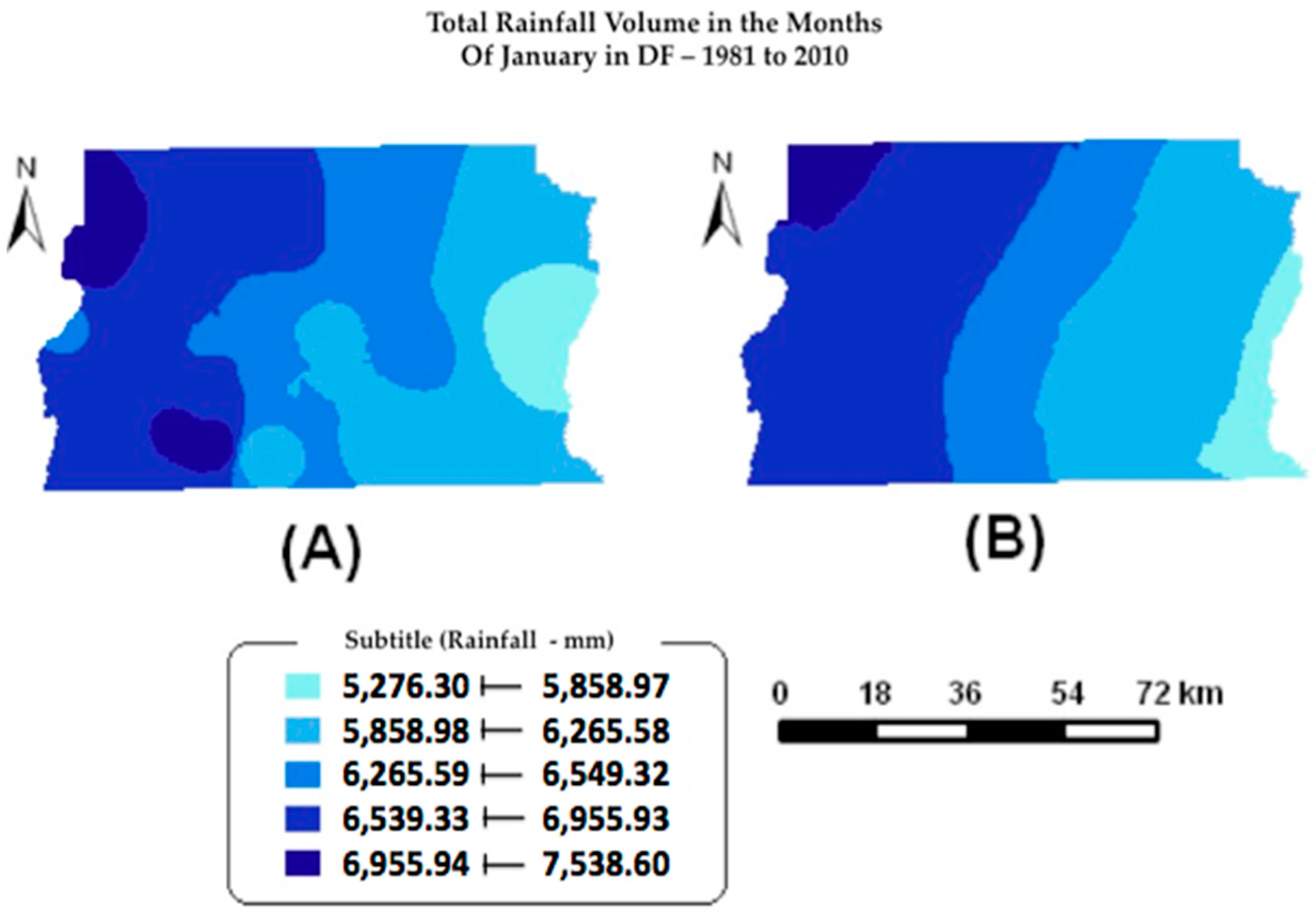
To observe the distribution of rainfall in the Federal District, the data were interpolated to map out the total volume of rainfall in the months of January from 1981 to 2010, based on the location of the 19 rain gauges. For comparative purposes, two interpolated maps were produced using different techniques: inverse distance weighted interpolation and ordinary kriging.
The number of class intervals of rainfall was calculated using Sturges’ formula [10], k = 1 + 3.3log(n), where k is the number of classes, log is the base-10 logarithm, and n is the number of observations. In the case in question, n = 19. Therefore, k = 5.22 ≈ 5. For both interpolation techniques, five intervals of rainfall were used. The results can be seen in Figure 8.
Based on the interpolated surfaces, an upward gradient of rainfall can be seen in a westerly direction. Using ordinary kriging (Figure 8B), five surfaces were produced that succeeded one another smoothly in a westerly direction. The same can be seen in Figure 8A, although inverse distance weighted interpolation yielded a less smooth succession, but still maintained an upward trend in the rainfall gradient in a westerly direction.
The midpoints between the upper and lower limits of the five class intervals in Figure 8 generated by the interpolation algorithms for the five classes were calculated (in rising order) as: 5567.64 mm, 6602.28 mm, 6407.45 mm, 6752.63 mm, and 7247.27 mm. The differences between the midpoints of each class and the class immediately below them were 494.64 mm, 345.18 mm, 345.18 mm, and 494.64 mm. In other words, it is fair to say that on average, the difference in volume between one surface and another is around 350–500 mm, which indicates a gradual, rather than abrupt, increase from one surface to the next.
The upward gradient in rainfall in a westerly direction corroborates the findings of [11,12,13]. According to Diniz [14], this fact is driven by three main factors: (1) much of the moisture that causes precipitation in the Federal District derives from a weather system that comes from the Amazon; (2) rain clouds are formed when cold fronts interact with humidity from the Amazon; and, (3) thermal convection, which is also responsible for rainfall, occurs more intensely in the western part of the Federal District, because this is the part with the highest levels of urbanization.
3.3. Dynamic of Rainfall Distribution at the 19 Rain Gauges
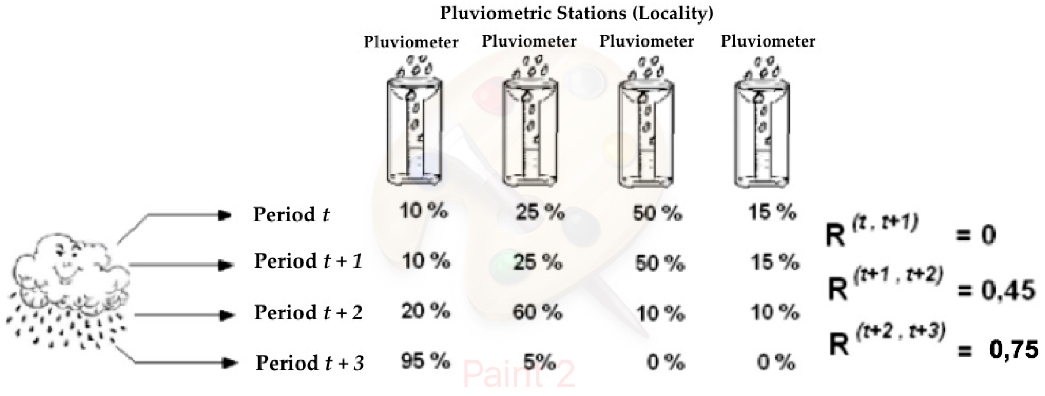
Another analysis was designed to ascertain the proportionality of rainfall distribution year on year at the 19 rain gauges. To measure the temporal dynamics of rainfall distribution at the gauges, the coefficient of redistribution (R(t,s)) was calculated. The formula for the coefficient of redistribution R(t,s) is given by:
where n is the number of rain gauges (in our case n = 19), t and s are two consecutive periods (for instance, t = January/1993 and s = January/1994), and x is the percent of rainfall in gauge station i at period t (or s). According to Souza (1977, p. 128), the value of this coefficient ranges from 0 to 1: 0 ≤ R(t,s) ≤ 1. If R(t,s) = 0, this means that the distributive structure of the phenomenon of interest in the space under analysis remained constant between period t and period s. The closer R(t,s) gets to 1, the greater the change in the distribution of the phenomenon of interest in the space under study, such that R(t,s) = 1 means complete redistribution; i.e., the phenomenon of interest is distributed completely differently between period s and period t. For illustrative purposes, Figure 9 shows a hypothetical example that indicates the calculated value of the coefficient of redistribution for four consecutive periods.
In the example in Figure 9, there is a significant redistribution of rainfall volume at the four sites between periods t + 2 and t + 3, whereas the pattern of rainfall distribution remains completely constant between periods t and t + 1. It is worth noting that the coefficient of redistribution does not consider the absolute value of rainfall from one year to the next, but the proportion of rainfall across the space, which in this case is the 19 rain gauges.
The coefficient of redistribution was calculated for rainfall at the 19 rain gauges, year by year, for the period running from 1981 to 2010. The calculated values of R(1981,1982), R(1982,1983), …, R(2009,2010) are presented in Figure 10.
Throughout the period in question, the coefficient of redistribution was relatively low. The mean value was 0.1363 and the highest value was R(1994,1993) = 0.2245. In view of the set of coefficients of redistribution calculated, the proportion of rainfall distribution at the 19 rain gauges can be considered to be stable between 1981 and 2010.
Finally, to assess the concentration or diversification of rainfall distribution at the 19 selected rain gauges in the Federal District in the months of January from 1981 to 2010, the Gini (G) and Gibbs-Martin (IGM) indices were calculated. According to Castro Filho, et al. [15], 0 ≤ IGM < 1. If IGM = 0, the volume of rainfall would all be concentrated at a single point, while a trend towards IGM = 1 would mean increasingly equidistributed rainfall at all 19 points. As for the Gini index, 0 ≤ G < 1 Souza, [16] such that G = 0 would indicate perfect equidistribution, while the closer G is to 1, the more spatially concentrated the phenomenon in question. The Gibbs-Martin index calculated for the distribution of rainfall at the 19 gauges in the months of January from 1981 to 2010 was IGM = 0.947, which indicates a strong trend towards equidistribution of the volume of rainfall throughout the space under analysis. Corroborating this finding, the Gini index was G = 0.047. A tendency towards equidistribution can also be seen from the Lorenz curve of the phenomenon. The more the Lorenz curve coincides with the equidistribution line, the greater the homogeneity of distribution of the phenomenon. Figure 11 shows the Lorenz curve almost coinciding with the equidistribution line, which indicates a strong trend in the period analyzed.
3.4. Descriptive Statistics for Rainfall Distribution in the Months of January from 1981 to 2010
In further analyses, some descriptive statistics were calculated for the rainfall in the 30 months of January at the 19 rain gauges. The results are presented in Figure 12. The amounts shown in Figure 12A are taken from the “Total Jan/year” column in Figure 6.
There are no outliers in Figure 12D. The distribution of the data in the stem-and-leaf diagram (Figure 12C) indicates bimodal data distribution, with 2200–2900 mm of precipitation falling in nine years and 4000 to 4700 mm falling in the other nine years. The amplitude of both ranges is around 700 mm. The variability of the data is moderate (Figure 12B) in view of the fact that the coefficient of variation (CV) is 35.99%. The coefficient of asymmetry (As) is 0.499, which indicates a positively skewed distribution, with a curve tending towards a platycurtic (plateau-like) distribution of data, since the coefficient of kurtosis (k) is 2.49. The bimodal nature of the data distribution is consistent with this result.
We could use the mean value of 4102.4 mm to represent the expected rainfall in January. However, given the bimodal distribution of the data, we propose taking the mean values of quartiles Q1 and Q3, as 50% of the values from the series are recorded in these quartiles. Thus, for practical purposes, we propose an expected rainfall of 3733.55 mm at the Federal District for January.
Inter-annual rainfall variability in the Federal District can be explained, according to Barros [13], by a number of atmospheric phenomena. However, the main factor behind the rainfall patterns in the region is the Atlantic Polar Anticyclone. When this Atlantic polar mass is stronger because of other atmospheric phenomena linked to the general circulation of the atmosphere, there is a higher volume of rainfall, while when this mass is weaker, the rainfall volume is lower.
3.5. Time Series of Rainfall at the 19 Rain Gauges in the Months of January from 1981 to 2010
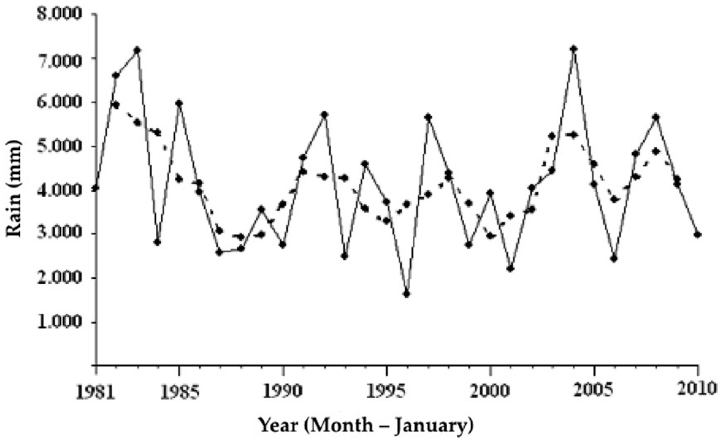
To analyze inter-annual variability of the volume of rainfall registered, the time series was analyzed to ascertain whether it contained any trends. To assess the existence of a trend in the time series, the first step was to make a visual inspection of the graphs of the time series and the series of third-order moving averages. Figure 13 shows both series.
From just visually inspecting the graph in Figure 13, it would seem that there is no trend in the time series. To check this, three nonparametric tests were conducted, as commented by Morettin and Toloi [17], namely: (1) a run test (Wald-Wolfowitz); (2) a sign test (Cox-Stuart); and (3) a test based on Spearman’s correlation coefficient. As well as these statistical tests, the Mann-Kendall test was also done. All of the tests used the same hypotheses: H0: null hypothesis (no trend in the series); H1: trend in the series.
The result of the Wald-Wolfowitz run test was not significant to the level of α = 5%, which means the null hypothesis was not rejected. The sign test yielded a p-value to the right of 15.09%, meaning that the test was significant to the level of α = 15.09%, which is very high. Therefore, the null hypothesis was not rejected. The test based on Spearman’s correlation coefficient yielded the statistical value t = −0.22269. To be significant to the level of α = 10%, the value would have to be tc = −1.313 or less. As t > tc, as in the other tests, this test was not significant and thus the null hypothesis was not rejected. Finally, when the Mann-Kendall test was done, this yielded a two-tailed p-value of 0.80276, which meant that the test was significant (accepting H1) up to α = 40%, which is extremely high. Therefore, the null hypothesis was also not rejected by this test.
All four tests of the statistical hypothesis led to the conclusion that there was no trend in the time series in question. Even so, a linear regression analysis was conducted of the original series and the third-order moving average data series. The linear regression estimates parameters β0 and β1 of the straight line Y = β0 + β1X.
For the original series, linear regression line Y = 35,880.89 − 15.91X. In other words, the angular coefficient of the straight line β1 was 15.91. However, when the hypothesis H0:β1 = 0 was tested against hypothesis H1:β1 ≠ 0, a p-value of 0.6194 was obtained, indicating a very high level of significance (α). Thus, the null hypothesis, where β1 = 0, was not rejected. This implies rejecting the existence of a slope in the regression line and rejecting the existence of a trend in the series. The regression analysis for the series of moving averages resulted in the regression equation Y = 18,506.644 − 7.208X. The hypothesis test yielded a p-value of 0.7118, which meant the null hypothesis was not rejected, and thus the non-existence of a trend in the series was implicitly accepted.
To conclude, the analyses indicated that the series from 1981 to 2010 was stationary, because none of the procedures used detected any trend in the series in question.
4. Discussion
The objective of this research was to perform a statistical experiment with rainfall data of the month of January of a period of 29 years. It was observed that there was no trend for rainfall in the study period. However, it is necessary to evaluate data from a time series that encompasses all 57 years of records and every month of the rainy season, which is from April to October, to verify if there is any trend in precipitation behavior. Evaluation of trends in time series, such as rainfall, is an important elemenet in hydrologic evaluations, including geomorphology elements [18,19] and planning efforts to avoid water shortages.
The proposed research is necessary at this moment, since the Federal District has been facing a water crisis since 2016. By obtaining the results of a more complete research, it will be possible to verify if the rainfall is directly influencing the water deficit or if there are other factors which must be taken into account. Through graphic representations, it will be possible to delimit periods essential for the performance of preventive actions and other measures of water management. With this type of approach it is possible to prevent the risk of water scarcity in the Federal District.
5. Conclusions
The exploratory analyses indicated a gently rising gradient of rainfall over the Federal District in a westerly direction in the months of January, taking into account five ranges, with an increase in mean rainfall from one range to the next of around 350–500 mm. Probably this rising gradient in the westerly direction is due, in part, to the fact that there is a greater concentration of stations in the western part of the territory. In addition, in the western region of the territory the highest geomorphological surfaces are presented above the altimetric elevation of 1000 m, reaching 1347 m. This may determine the occurrence of orographic rain in this region contributing to the higher volume of rainfall. The low coefficients of redistribution calculated indicate that there is little variation in the proportion of rainfall in the geographic space of the Federal District from one year to the next; in other words, the different geographic spaces in the Federal District (in this study represented by 19 gauges) received practically the same “percentage share” of the total volume of rain received in the previous year, year on year. Finally, there was no trend in the time series, which means that inter-annual rainfall variability in January must in fact be inherent to the climatic conditions.
Acknowledgments
The authors wish to thank CAESB (Company of Environmental Sanitation of Federal District) for the historical data series on monthly rainfall from the 27 rain gauges in the Federal District and adjacent areas, which were essential for this study.
Author Contributions
Valdir Adilson Steinke, theoretical methodological conception of the article, writing and final revision of the statistical treatment and results. Luis Alberto Palhares de Melo, procedures and statistical analysis of the time series, writing of methodological procedures and results. Ercília Torres Steinke, conceptual and methodological review, contribution in the final writing of the paper.
Conflicts of Interest
The authors declare no conflict of interest.
References
- Andrade, N.L.R.; Xavier, F.V.; Alves, E.C.F.R.; Silveira, A.; Oliveira, C.U.R. Caracterização Morfométrica e Pluviométrica da Bacia do Rio Manso—MT, Geociências; Rio Claro: Antioquia, Colombia, 2008; pp. 237–248. [Google Scholar]
- Setti, A.A.; Lima, J.E.F.W.; Chaves, A.G.M.; Pereira, I.C. Introdução ao Gerenciamento de Recursos Hídricos, 2nd ed.; Agência Nacional de Energia Elétrica, Superintendência de Estudos e Informações Hidrológicas: Brasília, Brazil, 2000. [Google Scholar]
- Lima, J.E.F.W. Determinação e Simulação da Evapotranspiração de Uma Bacia Hidrográfica do Cerrado; Universidade de Brasília: Brasília, Brazil, 2000. [Google Scholar]
- Campos, J.E.G. Hidrogeologia do Distrito Federal: Bases Para a Gestão dos Recursos Hídricos Subterrâneos; Revista Brasileira de Geociências: São Paulo, Brazil, 2004. [Google Scholar]
- Ramos, A.M.; dos Santos, L.A.R.; Fortes, L.T.G. Normais Climatológicas do Brasil: 1961–1990; INMET: Brasília, Brazil, 2009. [Google Scholar]
- Da Anunciação, Y.M.T. Regimes de Tempo e Precipitação Extrema de Verão Observados e Simulados na Região Central do Brasil. 101 f. (PHD in Geoscienses) Tese, Instituto de Geociências, Universidade de Brasília, Brasília, Brazil, 2013. [Google Scholar]
- Steinke, V.A.; Steinke, E.T.; Saito, C.H. Estimativa Da Temperatura De Superfície Em Áreas Urbanas Em Processo De Consolidação: Reflexões E Experimento Em Planaltina-DF. Rev. Bras. Climatol. 2010, 6, 37–56. [Google Scholar]
- Reinke, C.P.; da Silveira, R.B.; Reinke, R.L. Estudo Preliminar do Início e Término da Estação Chuvosa em Brasília. Available online: http://www.cbmet2010.com/anais/ (accessed on 22 November 2012).
- Oliveira, L.F.C.; Fioreze, A.P.; Medeiros, M.M.; Silva, M.A.S. Comparação de Metodologias de Preenchimento de Falhas de Séries Históricas de Precipitação Pluvial Annual; Revista Brasileira de Engenharia Agrícola e Ambiental: Campina Grande, Brazil, 2010. [Google Scholar]
- Gerardi, L.H.O.; Silva, B.C.N. Quantificação em Geografia; Difel: São Paulo, Brazil, 1981. [Google Scholar]
- IEMA/SEMATEC/UnB. Inventário Hidrogeológico e dos Recursos Hídricos Superficiais do Distrito Federal; IEMA/SEMATEC/UnB: Brasília, Brazil, 1998. [Google Scholar]
- Steinke, V.A.; e Steinke, E.T. Variação espaço-temporal da pluviosidade no Distrito Federal e seus condicionantes. In Simpósio Brasileiro De Climatologia Geográfica; 1 CD ROM; UFRJ: Rio de Janeiro, Brazil, 2001; pp. 21–31. [Google Scholar]
- Barros, J.R. A Chuva no Distrito Federal: O Regime e as Excepcionalidades do Ritmo. Rio Claro. 221 f. (Mestrado) Dissertação, Instituto de Geociências e Ciências Exatas, Departamento de Geografia, Universidade Estadual Paulista, Brasília, Brazil, 2003. [Google Scholar]
- Diniz, F.A. O clima de Brasília. In Disquete, Power Point, Palestra Proferida na Semana Meteorológica; INMET: Brasília, Brazil, 2004. [Google Scholar]
- Castro Filho, H.C.; Steinke, E.T.; Steinke, V.A. Análise espacial da precipitação pluviométrica na bacia do lago paranoá comparação de métodos de interpolação. Rev. Geon. 2012, 1, 336–345. [Google Scholar]
- Souza, J. Estatística Econômica e Social; Campus: Rio de Janeiro, Brazil, 1977. [Google Scholar]
- Morettin, P.A.; Toloi, C.M. Séries Temporais; Atual: São Paulo, Brazil, 1986. [Google Scholar]
- Steinke, V.A.; Sano, E.E. Semi-automatic identification, gis-based morphometry of geomorphic features of federal district of Brazil. Rev. Brasil. Geomorfol. 2011, 12, 3–9. [Google Scholar] [CrossRef]
- Steinke, V.A.; Pinto, M.L.C.; Araújo Neto, M.D.; Steinke, E.T. Proposed Relief Map of the Suitability of the Maranhão River Basin, Brazil, for Anthropogenic Use. J. Geogr. Inf. Syst. 2016, 8, 351–360. [Google Scholar]
Figure 1.
Climate normal for 1961–1990 showing accumulated monthly precipitation (mm) at the Brasília station (code 83.377). Source: [5].
Figure 1.
Climate normal for 1961–1990 showing accumulated monthly precipitation (mm) at the Brasília station (code 83.377). Source: [5].
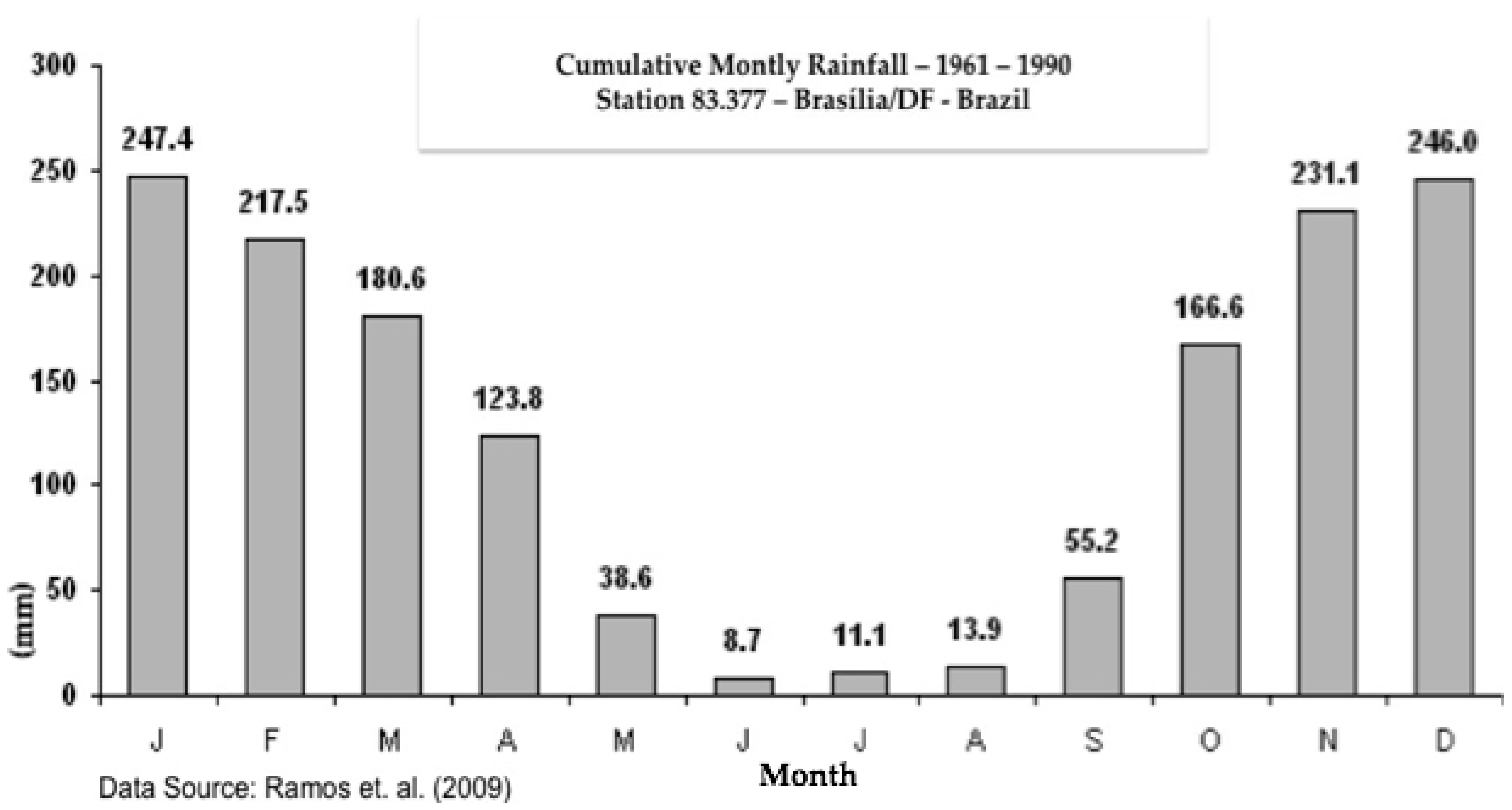
Figure 2.
(A) Geographic distribution of all 27 Companhia de Águas e Esgotos de Brasília (CAESB) rain gauges; (B) geographic distribution of the 19 CAESB rain gauges effectively used in this study.
Figure 2.
(A) Geographic distribution of all 27 Companhia de Águas e Esgotos de Brasília (CAESB) rain gauges; (B) geographic distribution of the 19 CAESB rain gauges effectively used in this study.

Figure 3.
Hypsometric map of Federal District of Brazil.
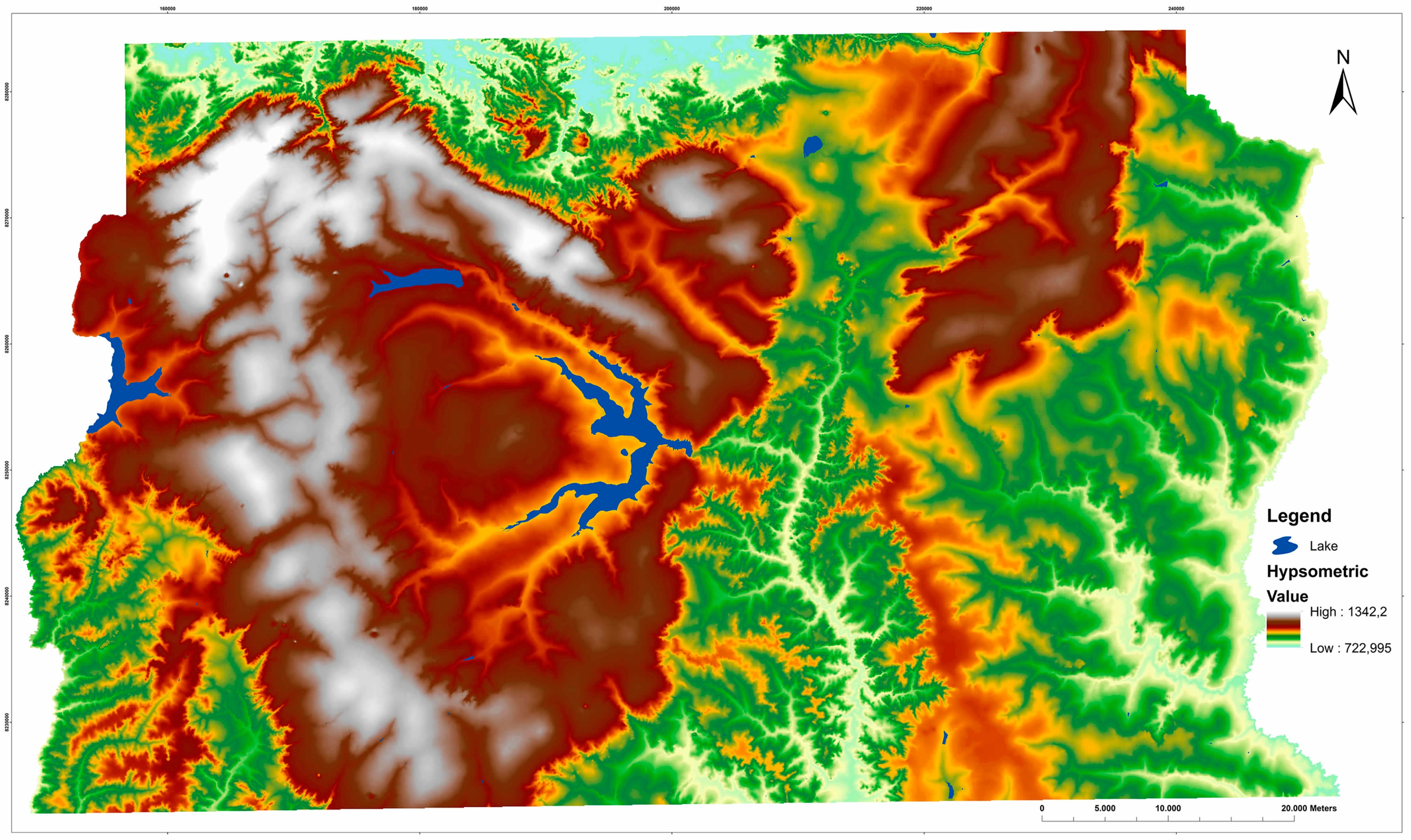
Figure 4.
(A) Calculation of the approximate (hatched) area of the Federal District using Quantum GIS (QGIS 2.0) software; (B) Calculation of the approximate (hatched) area of the 19 rain gauges using QGIS 2.0 software.
Figure 4.
(A) Calculation of the approximate (hatched) area of the Federal District using Quantum GIS (QGIS 2.0) software; (B) Calculation of the approximate (hatched) area of the 19 rain gauges using QGIS 2.0 software.
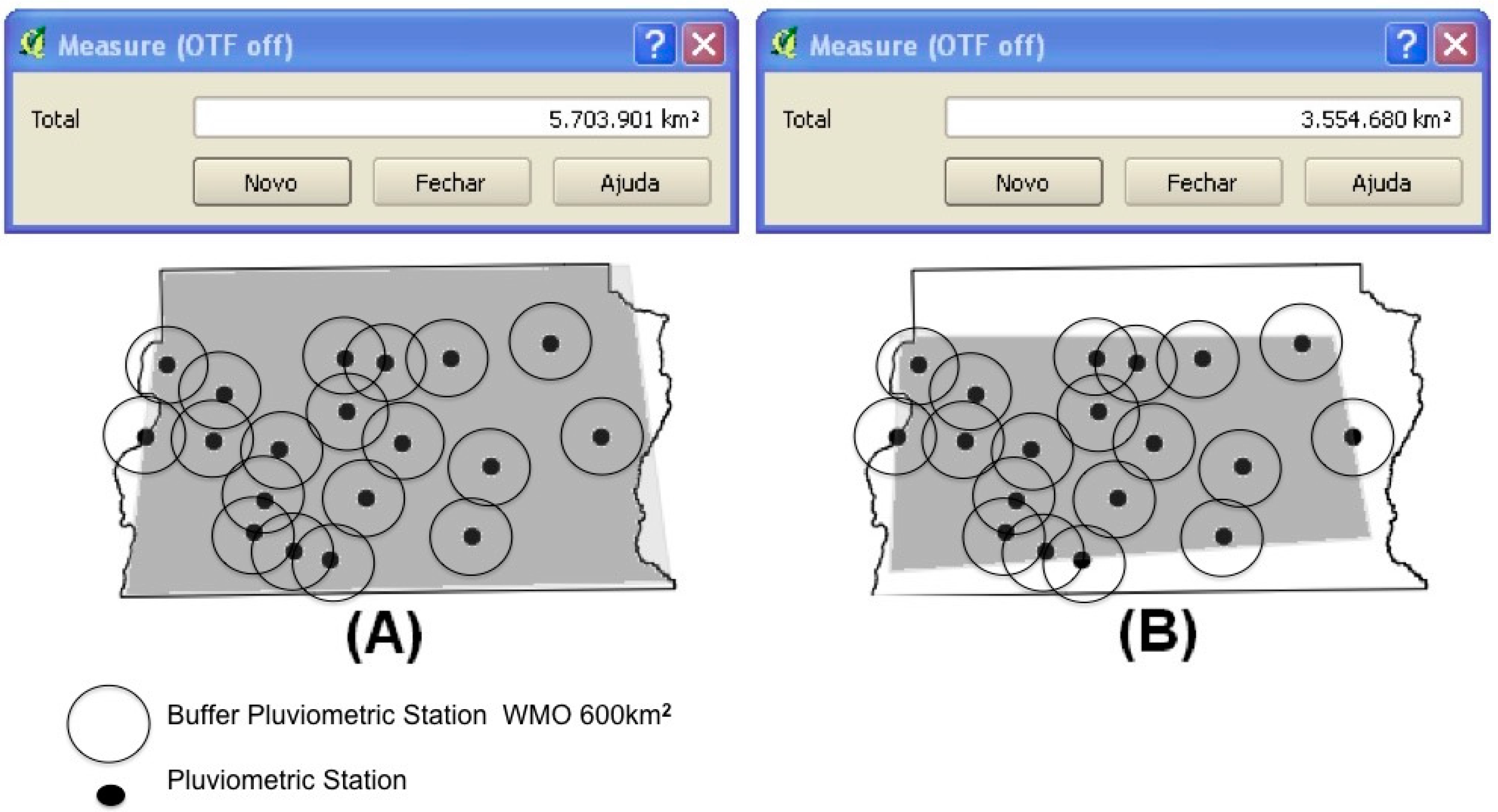
Figure 5.
Three point patterns in the Federal District. (A) Hypothetical distribution of the 19 gauges where they are very close together (clustered); (B) real pattern of distribution of the 19 gauges; and, (C) hypothetical distribution of the 19 gauges with a strong tendency toward dispersion.
Figure 5.
Three point patterns in the Federal District. (A) Hypothetical distribution of the 19 gauges where they are very close together (clustered); (B) real pattern of distribution of the 19 gauges; and, (C) hypothetical distribution of the 19 gauges with a strong tendency toward dispersion.

Figure 6.
Shortened table of monthly rainfall data at 19 rain gauges in the Federal District in the months of January from 1981 to 2010.
Figure 6.
Shortened table of monthly rainfall data at 19 rain gauges in the Federal District in the months of January from 1981 to 2010.
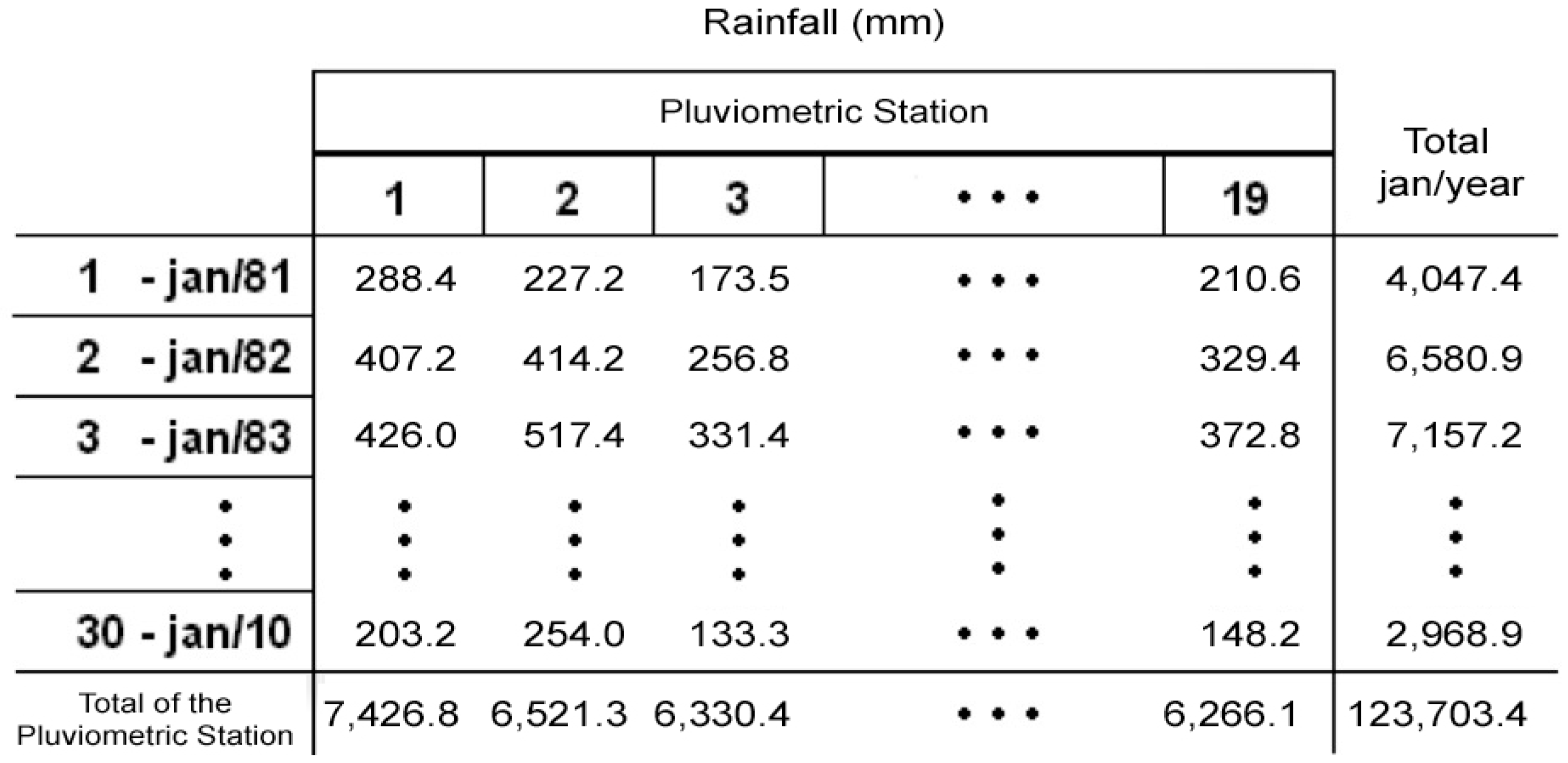
Figure 7.
(A) Total precipitation at the 19 rain gauges in the months of January from 1981 to 2010; (B) some descriptive statistics of the data series; (C) stem-and-leaf diagram of the data series; and, (D) box plot of the data series.
Figure 7.
(A) Total precipitation at the 19 rain gauges in the months of January from 1981 to 2010; (B) some descriptive statistics of the data series; (C) stem-and-leaf diagram of the data series; and, (D) box plot of the data series.

Figure 8.
(A) Surface interpolation using inverse distance weighting; (B) surface interpolation using ordinary kriging.
Figure 8.
(A) Surface interpolation using inverse distance weighting; (B) surface interpolation using ordinary kriging.

Figure 9.
Example of values for the coefficient of redistribution (R) for periods t, t + 1, t + 2, and t + 3.
Figure 9.
Example of values for the coefficient of redistribution (R) for periods t, t + 1, t + 2, and t + 3.

Figure 10.
Coefficients of redistribution R(1981,1982), R(1982,1983), …, R(2009,2010), for the space covered by the 19 rain gauges.
Figure 10.
Coefficients of redistribution R(1981,1982), R(1982,1983), …, R(2009,2010), for the space covered by the 19 rain gauges.
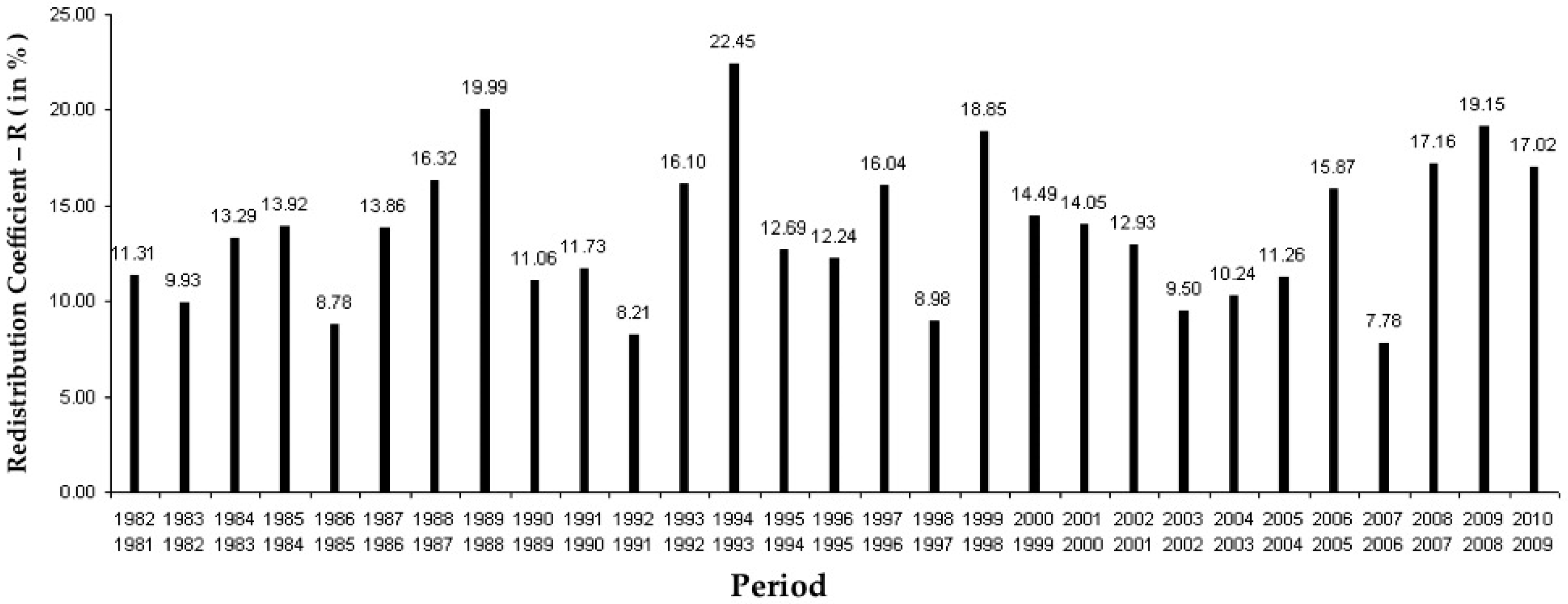
Figure 11.
Lorenz curve of the distribution of rainfall at the 19 rain gauges in the months of January from 1981 to 2010.
Figure 11.
Lorenz curve of the distribution of rainfall at the 19 rain gauges in the months of January from 1981 to 2010.
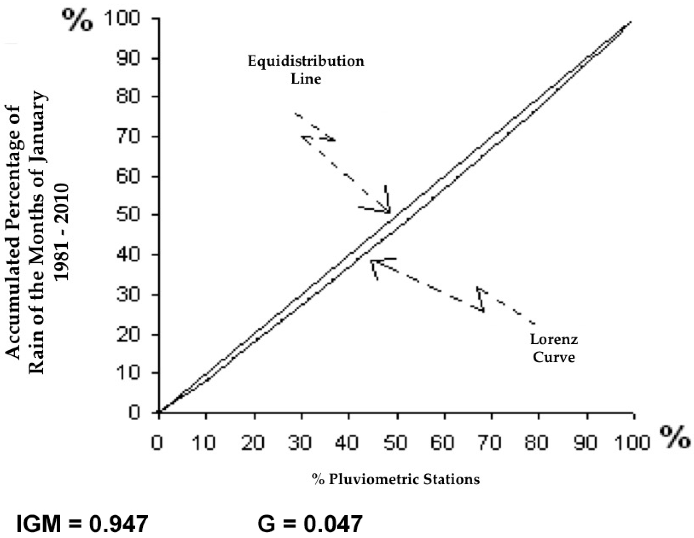
Figure 12.
(A) Total rainfall at the 19 rain gauges in the months of January from 1981 to 2010; (B) some descriptive statistics of the data series; (C) stem-and-leaf diagram of the data series; and, (D) box plot of the data series.
Figure 12.
(A) Total rainfall at the 19 rain gauges in the months of January from 1981 to 2010; (B) some descriptive statistics of the data series; (C) stem-and-leaf diagram of the data series; and, (D) box plot of the data series.
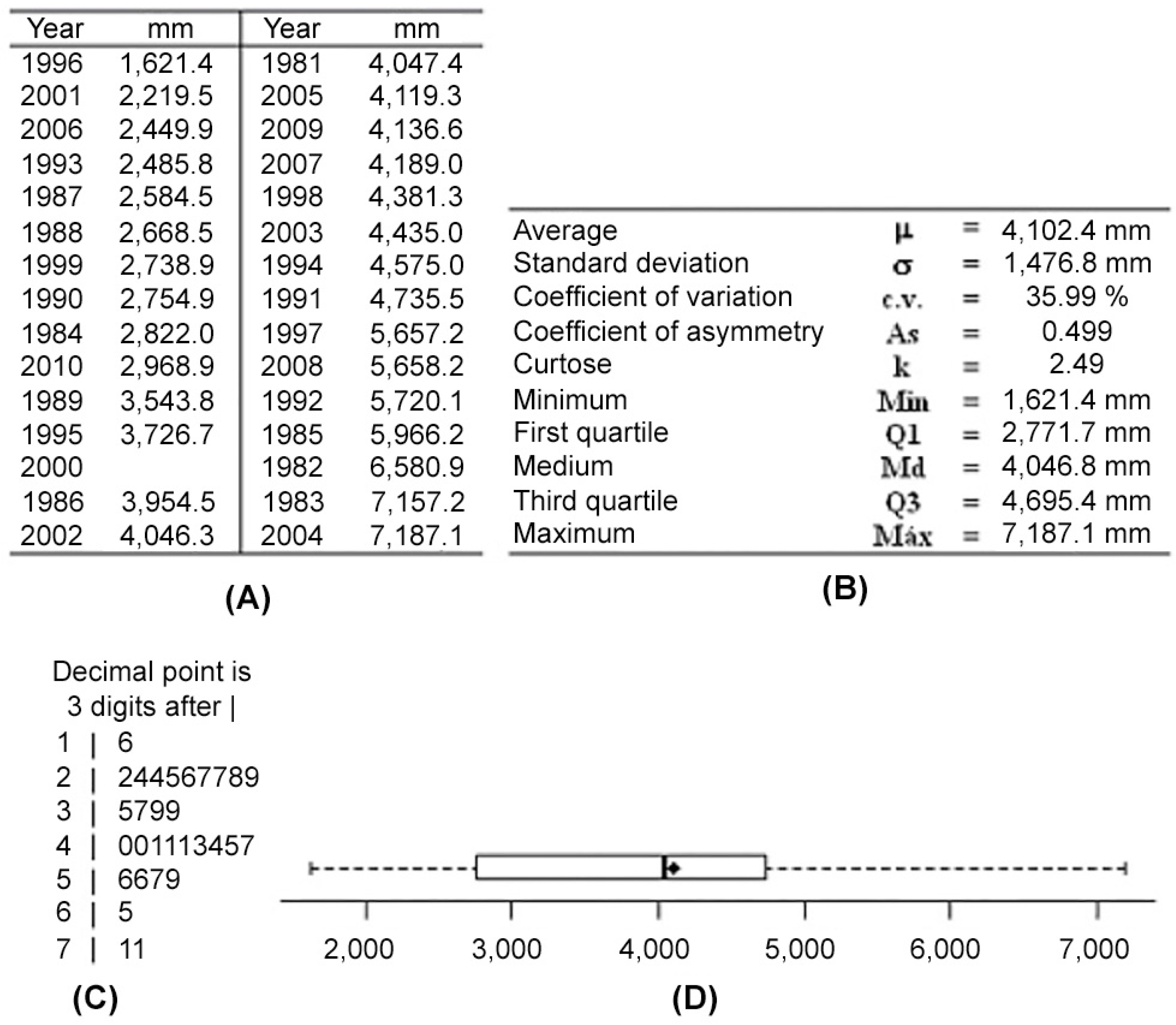
Figure 13.
Time series of rainfall (in mm) at 19 rain gauges in the Federal District in the months of January from 1981 to 2010 (unbroken line) and time series of the third-order moving averages (dashed line).
Figure 13.
Time series of rainfall (in mm) at 19 rain gauges in the Federal District in the months of January from 1981 to 2010 (unbroken line) and time series of the third-order moving averages (dashed line).

© 2017 by the authors. Licensee MDPI, Basel, Switzerland. This article is an open access article distributed under the terms and conditions of the Creative Commons Attribution (CC BY) license (http://creativecommons.org/licenses/by/4.0/).
Share and Cite
MDPI and ACS Style
Steinke, V.A.; Palhares de Melo, L.A.M.; Torres Steinke, E. Rainfall Variability in January in the Federal District of Brazil from 1981 to 2010. Climate 2017, 5, 68. https://doi.org/10.3390/cli5030068
AMA Style
Steinke VA, Palhares de Melo LAM, Torres Steinke E. Rainfall Variability in January in the Federal District of Brazil from 1981 to 2010. Climate. 2017; 5(3):68. https://doi.org/10.3390/cli5030068
Chicago/Turabian StyleSteinke, Valdir Adilson, Luis Alberto Martins Palhares de Melo, and Ercília Torres Steinke. 2017. "Rainfall Variability in January in the Federal District of Brazil from 1981 to 2010" Climate 5, no. 3: 68. https://doi.org/10.3390/cli5030068
Note that from the first issue of 2016, this journal uses article numbers instead of page numbers. See further details here.