Article

A Study of the Oklahoma City Urban Heat Island Effect Using a WRF/Single-Layer Urban Canopy Model, a Joint Urban 2003 Field Campaign, and MODIS Satellite Observations

1
SpringGem Weather Information
2
Department of Atmospheric and Oceanic Science, University of Maryland, College Park, MD 20742, USA
3
Department of Meteorology and Climate Science, San José State University, San Jose, CA 95192, USA
*
Author to whom correspondence should be addressed.
Climate 2017, 5(3), 72; https://doi.org/10.3390/cli5030072
Submission received: 23 June 2017 / Revised: 25 August 2017 / Accepted: 27 August 2017 / Published: 7 September 2017

Abstract

:
The urban heat island effect (UHI) for inner land regions was investigated using satellite data, ground observations, and simulations with an Single-Layer Urban Canopy Parameterization (SLUCP) coupled into the regional Weather Research Forecasting model (WRF, http://wrf-model.org/index.php). Specifically, using the satellite-observed surface skin temperatures (Tskin), the intensity of the UHI was first compared for two inland cities (Xi’an City, China, and Oklahoma City (OKC)), which have different city populations and building densities. The larger population density and larger building density in Xi’an lead to a stronger skin-level UHI by 2 °C. However, the ground observed 2 m surface air temperature (Tair) observations showed an urban cooling island effect (UCI) over the downtown region in OKC during the daytime of 19 July 2003, from a DOE field campaign (Joint Urban 2003). To understand this contrast between satellite-based Tskin and ground-based Tair, a sensitivity study using WRF/SLUCP was analyzed. The model reproduced a UCI in OKC. Furthermore, WRF/Noah/SLUCM simulations were also compared with the Joint Urban 2003 ground observations, including wind speeds, wind directions, and energy fluxes. Although the WRF/SLUCM model failed to simulate these variables accurately, it reproduced the diurnal variations of surface temperatures, wind speeds, wind directions, and energy fluxes reasonably well.

1. Introduction

Earth, as a physical system, is balanced by incoming energy and outgoing energy. For an equilibrium climate, the mean global absorbed solar shortwave radiation is balanced by the outgoing long-wave radiation. In general, in the Earth system, 19% of the incoming solar radiation is absorbed in the atmosphere, 30% is lost to space, and 51% is absorbed at the surface. This last component of the incoming radiation, along with the outgoing sensible and latent heat fluxes, is the main contributor to the surface skin temperature [1,2].
Surface temperature normally presents heat at a particular location on the Earth surface. From the satellite view, the “surface” is defined as whatever ground-level information that is transmitted through the atmosphere. Consequently, surface temperatures retrieved from satellite observations are called “surface skin temperature (Tskin)” [3]. Tskin represents the ground temperature when the underlying surface below the satellite is bare soil, or represents the canopy top temperature when the underlying surface is forest. For an urban area, Tskin is the mixed signal of building tops, building walls, streets, and parks that are seen by satellite within its view angle. For comparison, the air temperature cited in daily weather reports, defined as the surface air temperature (Tair) and observed in a weather shelter positioned at ~2 m height above the surface, differs from Tskin in both physical meaning and magnitude [2,4].
Urbanization usually leads to significant changes in the surface and atmospheric boundary-layer properties, creating an urban micro-climate [5,6,7]. This includes the urban heat island effect (UHI): a phenomenon in which the 2 m Tair in an urban area is usually higher than that in an adjacent rural area, with a greater temperature difference during nighttime than during daytime [5,6]. Jin et al. [8] shows, on Tskin, that the UHI is even stronger in this skin-level of temperature and that the daytime has a larger UHI signal than the nighttime. The differences between UHI on Tair and Tskin has received a great amount of attention because the impact of the UHI is increasingly becoming a global concern. About half of the world’s human population lives in urban areas and the population migration from rural to urban areas continue. The UHI affects the weather in urban regions by modifying surface temperature, pollution, and precipitation, and thus can affect human health [9,10]. For example, an increased frequency of heat waves in urban regions leads to heat-related illness and even death [9]. Therefore, in recent years, numerous studies on UHI impacts, focusing on human health, have been carried out [11].
Studies on UHI predominantly use three different approaches: ground observations, satellite observations, and model simulations [12,13,14,15,16,17,18,19,20,21,22,23,24]. For example, using the Tair data from meteorological stations over the last century, Montavez et al. [25] examined the UHI of Granada data and revealed an increasing trend in the minimum Tair and a decreasing trend in the maximum Tair. In addition, comparison of urban and rural temperatures revealed a stronger UHI in winter, with a maximum difference in the early morning. In their work, Montavez et al. [25] also examined the urban geometry impact on UHI. In a more recent study, Hamdi and Van de Vyver [26] estimated the UHI in Brussels by using the surface temperature data from ground-based weather stations and remote sensing data from the years 1955 to 2006, also showing that the growing rate of the urban effect on minimum Tair is about 2.5 times more than that on maximum Tair.
The Weather Research and Forecasting (WRF) model was used by Yang et al. [27] to investigate the UHI. The authors studied the urban climate in Nanjing, a large city in Eastern China, using a 1 km resolution WRF model coupled with a single-layer Urban Canopy Model. They concluded that the WRF model was suitable for simulation of surface air temperature, relative humidity, and precipitation frequency, although it underestimated the total amount of precipitation in Nanjing. Chen et al. [28] studied the UHI phenomena over the greater Houston area by using the coupled WRF/LSM/Urban Modeling system simulation. Their aim was to develop a more complex urban canopy model in WRF, with a more detailed description of urban land cover types. Salamanca et al. [29] studied the urban boundary layer using high-resolution urban canopy parameters with WRF. By comparing the results from their case study, the authors concluded that a complex urban canopy scheme and detailed urban canopy parameters are needed for the simulation due to the air conditioning at the city scale. The WRF model is a valuable tool for understanding and predicting the effects of climate change, and simulating the meteorological conditions from building to regional scales.
Satellite observations, such as the Moderate-resolution Imaging Spectroradiometer (MODIS), are characterized by high spatial and temporal resolution (i.e., 1 km, 2-time/day), global coverage, and high quality observations. Therefore, satellite data are useful for studying the land surface climate. These observations can provide significant amounts of surface data at a relatively low cost, and can thus be appropriate for studying long-term, large-scale atmospheric and surface changes.
Limits exist in all remote sensing, ground, and model approaches. For example, MODIS observations of Tskin are available only for clear days because only IR channels are used to retrieve surface temperature and MODIS cannot detect surface variables through clouds. In addition, while the air temperature data obtained from weather station ground observations is useful to examine long-term changes, it may not be suitable for studying high heterogeneous urban regions due to the low spatial resolution of weather sites. Finally, model simulations are based on a current understanding of the phenomena of interest, which is normally not adequate, so model simulations have numerous uncertainties and thus may not be able to capture the influences of city structures accurately due to the heterogeneity of urban areas.
The physical mechanisms of the UHI has been a research topic for decades [5,6,7]. For example, the heat capacity of materials used in urban construction is much greater than that of the original vegetation in the forests and other natural features. As a result, urban structures that absorb a large amount of thermal energy during daytime and slowly emit the stored heat during late afternoon and nighttime. Furthermore, evapotranspiration, a process that converts liquid-water to water vapor as a natural cooling mechanism, is limited on urban impervious surfaces. In addition, tall buildings in urban regions increase the surface roughness and enhance turbulence of the surface-boundary layer [30]. As a result, buildings lift the air and result in convection. Consequently, buildings often modify the original air flow direction, trap aerosols, increase pollution in the urban system, and degrade air quality [31]. Furthermore, urban construction creates an urban “canopy” geometry, reducing the surface albedo and altering the emissivity in urban regions [10]. Lower albedo increases solar radiation absorption in cities. Besides these effects, walls of the buildings extend the effective urban surface, so that the more buildings there are, the more shortwave radiation is absorbed.
The Urban Cooling Island effect (UCI), which is when the surface temperature over urban regions is lower than that in the surrounding rural regions, has also been discussed [32]. The mechanisms for UCI are presently unclear. It was speculated that the aerosol direct effect reduces surface insolation and thus may lead to a UCI. Nevertheless, Jin and Shepherd [32] assessed the urban aerosol direct effect over Beijing, New York City, Mexico City, and Moscow from remote sensing data combined with a WRF model sensitivity study on the urban skin temperature. Their study found that, while urban aerosols reduce both Tskin and Tair, the magnitude of the reduction is insufficient to offset the UHI induced by other mechanisms including surface albedo reduction (Jin and Shepherd 2008). Furthermore, Jin et al. [10] carried out a similar land–atmosphere interaction study for Shanghai—one of the biggest, most densely populated urban cities in China. This study found a similar conclusion for the impacts of aerosol’s direct effect on UHI in Shanghai. Nevertheless, the authors proposed another mechanism for a UCI: building shadows reducing surface insolation. In addition, urban buildings can change the wind vector and thus enhance the eddy mechanic turbulence. As a result, heat at the ground was transported to the higher air levels, which consequently reduced surface temperature. In the study presented in this paper, the UCI was occurred from ground observations as well as on WRF simulations during daytime, suggesting that building shadow may be the key reason for UCI.
This study aimed to analyze the physical process of the UHI/UCI as well as determine whether the WRF/Single-Layer Urban Canopy Model (SLUCM) simulation can successfully reproduce the UHI/UCI. Two cities, Xi’an City in China (34.0°–34.6° N, 108.6°–109.2° E) and Oklahoma City (OKC, 35.2°–35.8° N, 97.2°–97.8° W) in the United States, were chosen to reveal the size and population impacts of urbanization. Both cities are inland at about the same latitude. Thus, the UHI of each city should be related to the geometric properties, with little or no effects from the ocean. However, Xi’an has an urban area of 319 sq. km with a population density of about 20,000/sq. km, while the urban area for OKC is 410.6 sq. km with a population density of about 2000/sq. km. Thus, Xi’an has a smaller urban area but a much larger population density.
From the 2 m Tair data and MODIS Tskin data, our work reveals that city characterized by dense urban buildings and population density, like Xi’an, has a much more significant UHI. Moreover, UHI signals on Tair is clearly different from that on Tskin. The UCI was observed in a downtown high building region from OKC field campaign on Tair data. However, the SLUCM coupled into WRF Noah Land Surface Model (Noah-LSM) decently captures the influences of urban properties. Nevertheless, the built-in United State Geological Survey (USGS) 24-category land-use data in WRF are outdated in many urban regions and cannot accurately represent the coverage of urban areas. In addition, the default building height for real urban cities is incorrect and certain physical processes need to be added in the urban model.

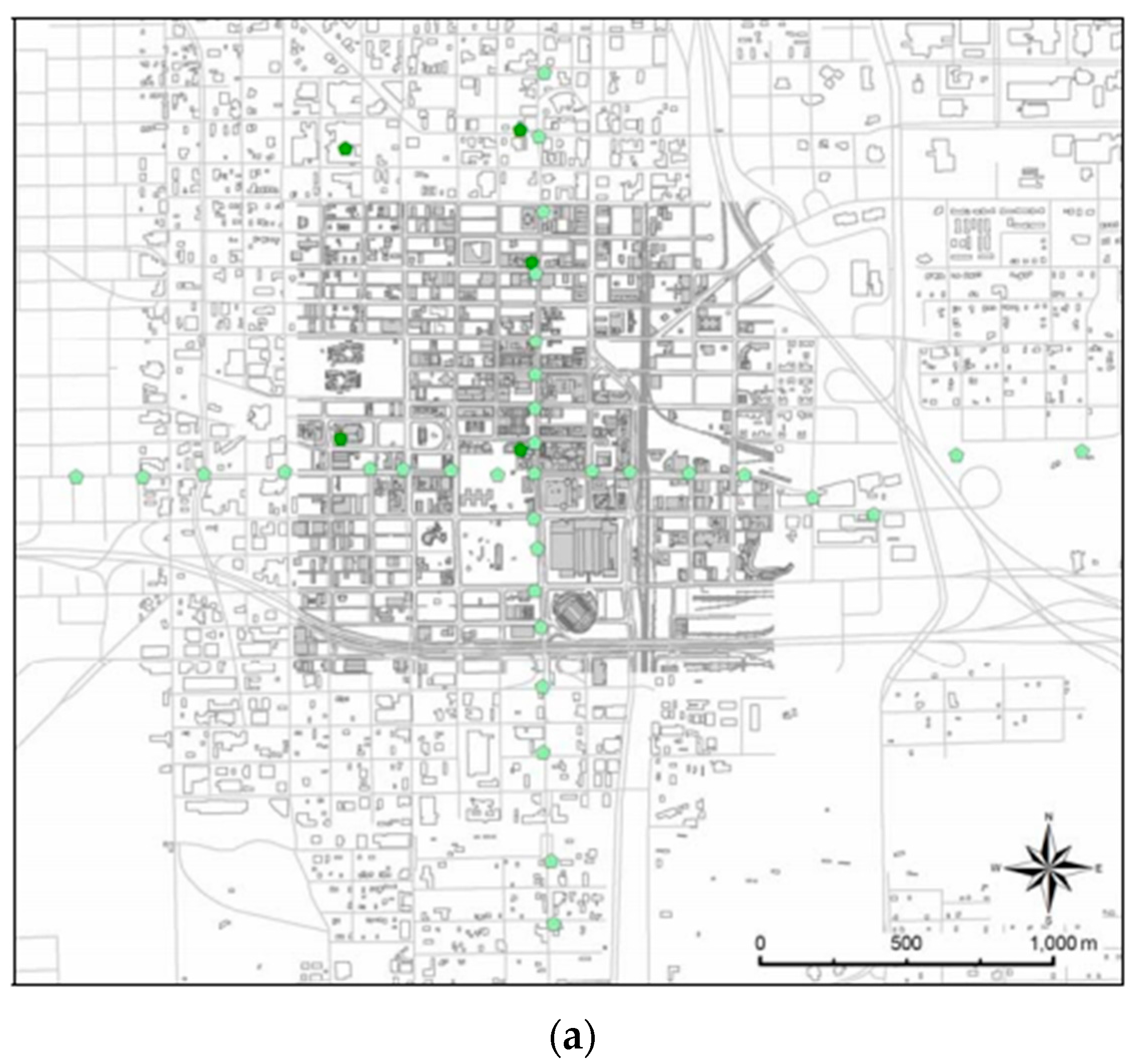
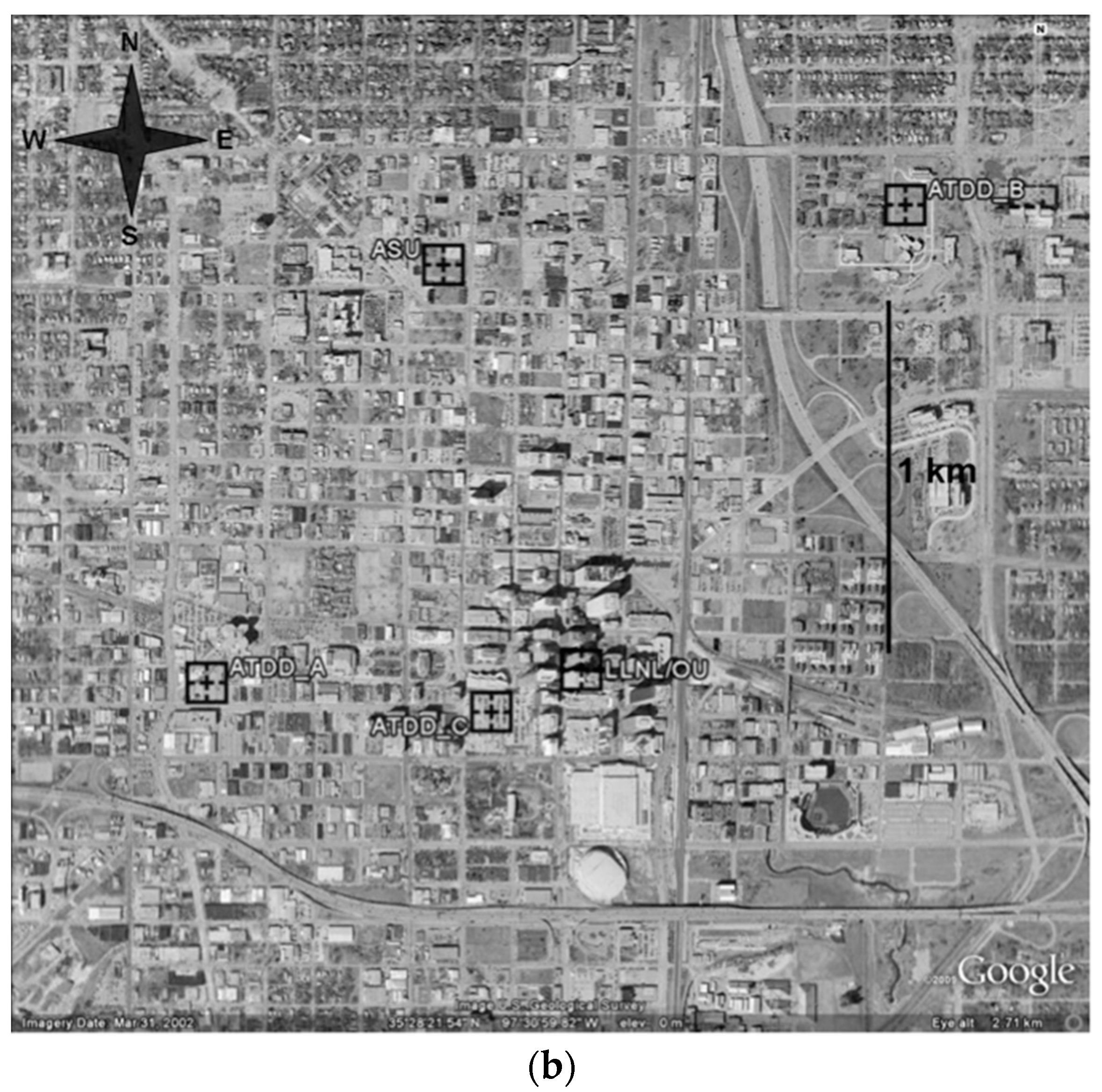
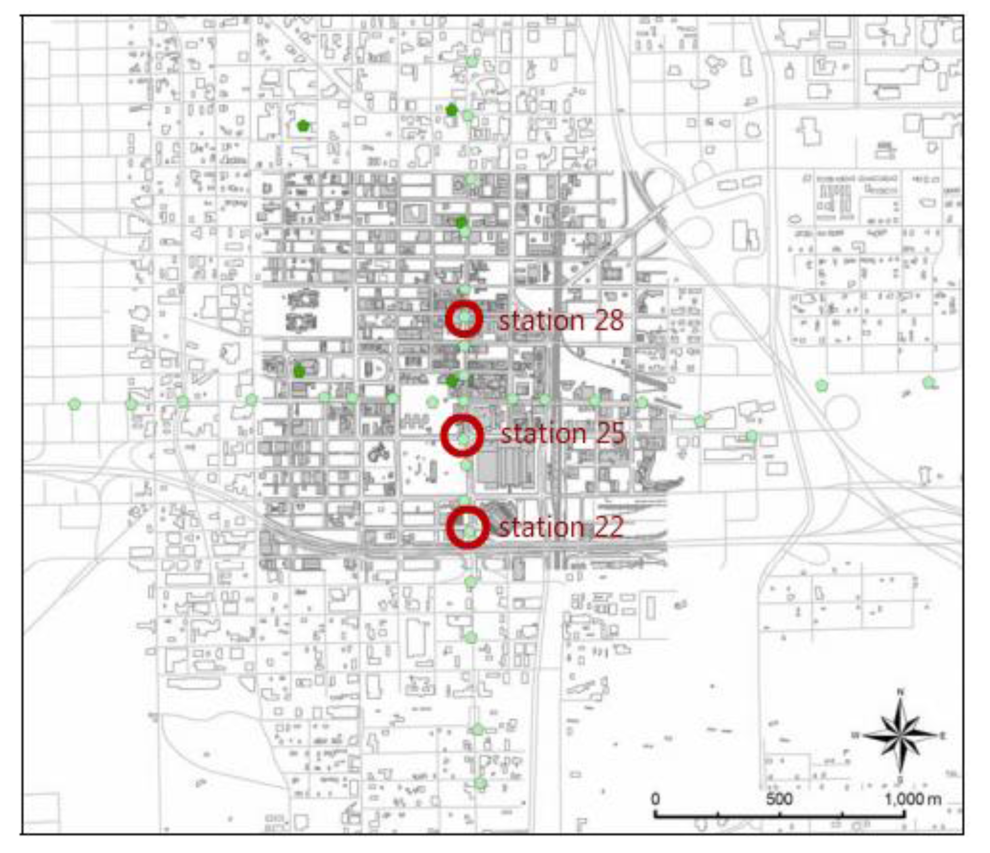
2. Joint Urban 2003 Field Campaign

The Joint Urban 2003 (JU2003) field campaign, sponsored by the U.S. Department of Defense, Defense Threat Reduction Agency, and the U.S. Department of Homeland Security, was conducted in Oklahoma City (OKC), Oklahoma from 28 June to 31 July 2003. Over 150 scientists and engineers as well as many foreign institutions participated in this project aiming to investigate the atmospheric dispersion in OKC [33]. Air temperature sensors, radiosondes, radars, lidars, sodars, and sonic anemometers were deployed as a part of this initiative, and the physical processes—including surface energy balance in the urban area, the flows within the tall-building areas and street canyons, the effects of traffic on turbulence, the development of urban boundary layer, and the dispersion of tracers—were studied. Large amounts of high-resolution data was collected, which resulted in hundreds of journal articles, presentations, and reports on this field project.
T Sourced from the JU2003 field project in OKC, the Pacific Northwest National Laboratory (PNNL) HOBO 2 m air temperature data and the Atmospheric Turbulence and Diffusion Division (ATDD) flux site data were used to study the synoptic situation of the UHI in OKC. The PNNL set up 33 temperature sensors in a cross-section through the Central Business District (CBD) of OKC (Figure 1a). More specifically, Sensors 1 through 17 were placed on Main Street, in the direction from west to east, while Sensors 18 through 33 were placed on Robinson Avenue, in the direction from south to north. Sensor 9 was thus located at the centermost point of the city. In addition, as each sensor was only one or two blocks away from the next one, high spatial resolution data could be measured. The 2 m air temperature data through the downtown OKC were collected from these HOBO stations [33]. In this paper, the 2 m air temperature from ground observations was first analyzed to demonstrate the building cooling effect on surface air temperature and then, compared to the WRF model simulation to validate the model performance on the urban effect.
The Atmospheric Turbulence and Diffusion Division (ATDD) deployed three surface flux sites, labeled as A, B, and C in Figure 1b to show their locations. Site A was located in a gravel and dirt parking lot in the west of the CBD of OKC, Site B was located northeast of CBD in a grassy area, and Site C was located on the top of a multiple-level concrete parking garage at the southwest corner of CBD (Hanna 2011, personal communication). Energy flux variables, such as net radiation, incoming shortwave radiation, sensible heat flux, and latent heat flux, were collected. In this research, the data obtained from Site A and Site B were excluded due to the unrealistically large value for the ground heat flux data observed from Site A, during nighttime, and the large latent heat flux value observed from Site B (Hanna et al. 2011). Consequently, the analyses performed in this study were based on the Site C data set, because all the flux measurements had reasonable values. Although the data set contained several variables, the present study mainly focused on net radiation, incoming shortwave radiation, wind speed, and wind direction.

3. Other Data and Methods

3.1. Satellite Observation

MODIS land cover data and the MODIS surface skin temperature (Tskin, 8) data were used in this study to identify the UHI in OKC and Xi’an city. The MODIS instrument that collected this data is mounted on NASA’s Aqua (EOS pm) and Terra (EOS am) satellites. The MODIS/Terra Land Cover Types Yearly L3 Global 0.05Deg CMG (MOD12C1) apparatus was used in this study to create land cover maps for OKC and Xi’an. This land cover classification method includes multiple classification schemes, such as International Geosphere-Biosphere Programme (IGBP) classification scheme. The IGBP contains three developed land classes, eleven natural vegetation classes, and two additional classification schemes at a 0.05° resolution. The vegetation classes are emphasized, but the vegetation mosaic, snow information, and wetlands are excluded. After creating land cover maps for OKC and Xi’an, the land cover types of urban regions and surrounding rural regions for both cities were compared. The MODIS11C3 Monthly CMG LST, which is the monthly daytime 3 min CMG land-surface temperature data, was used in this research. The values of the land-surface temperature are those observed in the 0.05° latitude/longitude grids (CMG). This UHI study was conducted from 2001 to 2008 at both daytime and nighttime in OKC and Xi’an.

3.2. WRF/Single-Layer Urban Canopy Model (SLUCM) Simulation

The Urban Canopy Model (UCM) is a single layer model (Figure 2a) coupled to the WRF model, and includes a 2-D street canyon. Figure 2b shows the radiation yielded by the single-layer urban canopy model (SLUCM), whereby SLUCM represents the physical process in the urban environment and provides better forecasts for urban areas. This urban scheme represents a simplified urban geometry, including the modification on wind profile in the urban “canopy” layer, surface albedo, and emissivity. The tall building shadow effect was simulated as shown in Figure 2b. Furthermore, human-induced heat fluxes that are transferred to roads, walls, and roofs are also added in the surface energy budget [34,35].
The state of the atmosphere is atmosphere forcing to feed into Noah/SLUCM. The output from the Noah/SLUCM feeds back to the WRF atmosphere scheme to update the atmospheric conditions, as designed in Kusaka et al. [34]. The surface parameters’ canyon dimensions used in the models and some key physical constants used in the models are listed in Table 1.
In this research, 24 h simulations of WRF/Noah began at 12:00 UTC (06:00 LST) on 19 July 2003, with the boundary conditions from NCEP North American Regional Reanalysis (NARR). The horizontal domain created for this simulation was comprised of three nested domains with a grid spacing of 25 km, 5 km, and 1 km (Figure 3).
Two simulations were performed: a control run without SLUCM and a sensitivity run with SLUCM. The control run is the default Noah surface scheme without an urban scheme specified. The sensitivity run is a Noah model coupled with SLUCM, in which urban physical and thermal-dynamic processes are described. The simulated Tskin over the urban regions in OKC for the sensitivity run was compared with the control run to show the performance of SLUCM. In addition, the simulated surface skin temperatures in the WRF/SLUCM between the urban region and rural region nearby OKC were compared to reveal SLUCM reproduction on urban effects. Furthermore, the WRF/SLUCM-simulated surface temperature wind speed and direction are validated using field ground observations.

4. Results

4.1. Satellite Observation

Xi’an City and OKC are both inland cities, located around 35° N, with similar cloud cover during July. Thus, they are expected to receive a similar amount of solar radiation. Nevertheless, MODIS land cover observations suggest that the surrounding land cover types of these two cities are not the same (Figure 4a,c) [36]. Specifically, there are more croplands (land cover = 12, cropland) and mixed forest (land cover = 5, mixed forest) surrounding Xi’an City, while OKC is mostly surrounded by grassland (land cover = 10, grassland) and croplands (land cover = 12, cropland). As a result, monthly Tskin varies with land cover types for both OKC and Xi’an City (Figure 4b,d). Evidently, Tskin over the urban area is much higher than the Tskin measured in the surrounding rural area for both cities. In OKC, Tskin of the urban area is about 299 K, while the Tskin of rural area is around 295–298 K. Similarly, in Xi’an City, the value of Tskin for urban and rural area is 308 K and 306 K, respectively.
The temperature difference is calculated based on the following expression:
Tdiff = Turban − Tnonurban
where Turban and Tnonurban indicate the surface skin temperature averaged over all urban/non-urban pixels, respectively, within the areas highlighted in the small boxes in Figure 4. Both OKC and Xi’an City have a significant UHI indicated by Tdiff (Figure 5). For OKC, the monthly Tdiff is always positive with a 0.5–4.4 °F range (Figure 5b), while for the nighttime, the Tdiff ranges from 0.6 to 3.0 °F (Figure 5d). In comparison, for Xi’an City, urban Tskin values are also higher than rural Tskin most of the year, except January (not shown) when the daytime Tdiff value ranged from −0.4 to 7.2 °F and the nighttime Tdiff ranged from 2.5 to 4.2 °F (not shown). More importantly, the UHI is stronger in warmer seasons than in colder periods. In addition, for OKC, the strongest daytime UHI occurred around May and the weakest UHI around December (Figure 5b). On the other hand, the strongest nighttime UHI was measured in July and the weakest UHI occurred around February (Figure 5d). Nevertheless, further analysis on clouds and rainfall is needed in order to fully understand such temporal differences.
Both daytime and nighttime Tdiff in Xi’an City are always higher than those in OKC (Figure 6a,b), especially during daytime of May and August. Tdiff in May for Xi’an City is about 7.8 °F, while for OKC it is about 3.9 °F. Moreover, Tdiff for Xi’an City measured in August is about 6.0 °F, while it is only 2.0 °F for OKC (Figure 6a). In addition, the nighttime differences are smaller than those found for the daytime temperatures (Figure 6b), which suggests that the UHI in Xi’an City is stronger and much more significant than that in OKC. This may be due to higher and more densely distributed buildings, and a larger population density in Xi’an City. Simply put, UHI is determined by the city characteristics (size, building density, population, etc.) and exhibits clear seasonality and diurnal features.

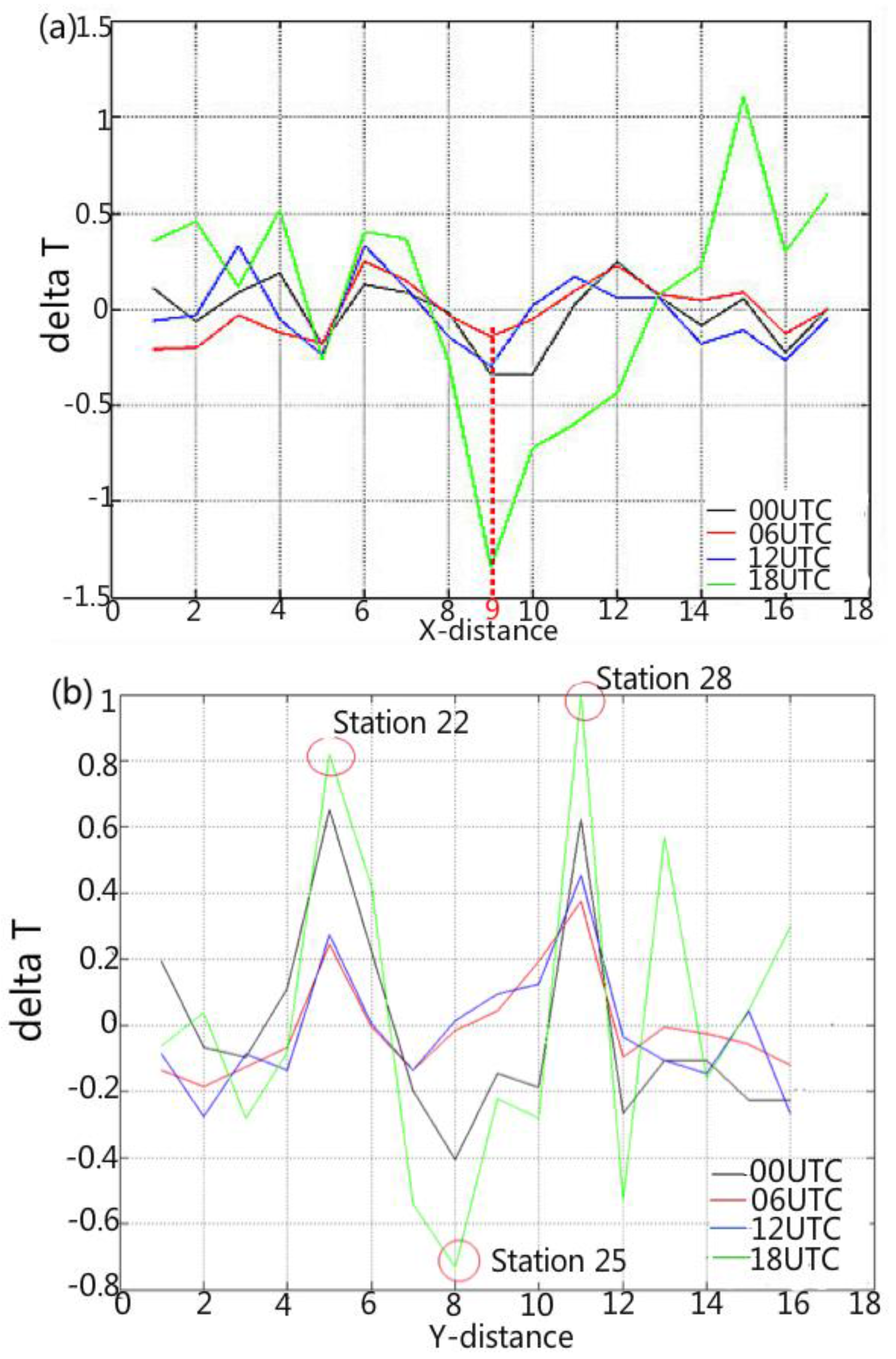
4.2. Ground Observations

The values of Δ T at the x-direction as well as for y-direction were calculated based on the equation:
ΔT = Ti − Tmean (i = 1, ..., 17 for the x-direction; i = 1, …, 16 for the y-direction
where Ti is the 2 m Tair collected from Station No. i (i = 1, …, 17 for the x-direction; i = 1–16 for the y-direction), and Tmean is the averaged 2 m Tair from all 17 or 16 stations in one direction. The temperature difference measured for the Station No. 9 was much lower than that observed at the other stations, especially at noon (Figure 7a). This feature may be due to the fact that Station No. 9 was located at the centermost point in OKC and surrounded by tall buildings. Consequently, less solar radiation can reach this station. Similarly, along the y-direction, Station 25 also has cooler than other stations. The greatest range of Tair among different stations occurred at noon when the incoming solar radiation is the strongest. In contrast, at around midnight, the temperature difference is reduced due to no surface insolation. Furthermore, at noon, the two highest values—0.8 °C and 1.0 °C—were obtained at Stations No. 22 and No. 28 (Figure 7b), respectively, while the lowest value (−0.7 °C) was recorded at Station No. 25. This evident cooling signal at the downtown regions may suggest an urban cooling effect (UCI), although no rural station data is available for assessment. In conclusion, the 0.5–1.5 °C difference at center downtown stations from other urban stations is critical for revealing that the urban high heterogeneity surfaces results in different UHI/UCI signals in different regions.
The diurnal cycles of Tair for Station No. 22, Station No. 25, and Station No. 28 were similar and were characterized by peak values at 3:00 p.m. and minimum values at 6:00 a.m. (Figure 8). However, Tair from Station No. 25 (red curve) was always below those Tair observed at the other two stations. This may be due to the fact that only Station No. 25 is located in the vicinity of the centermost point in the OKC town center (see Figure 9). Tall buildings in the downtown center exhibit several important effects that contribute to this feature by blocking sunshine and casting shadows on Station No. 25. In addition, the walls of tall buildings lift air parcels (a dynamic mechanism similar to mountain lift) and increase local circulation. This process enhances eddy turbulence and transports heat from the ground surface to the higher air levels. As a result of all these mechanisms, the air temperature at Station No. 25 is reduced. More importantly, measurements obtained at Stations No. 9 and No. 25 reveal that OKC has a UCI. This new and important feature, which was not observed from the Tskin field, may imply the difference between Tair and Tskin in terms of physical effects and magnitudes (Jin and Dickinson 2010). Furthermore, satellite-based Tskin is under a satellite field view and has a monthly, 1 km resolution, while the Tair observation is in situ. The differences in spatial and temporal resolution may be useful to reveal the details of Tskin and Tair. Tskin and Tair.
The soil temperatures at 32 cm and 64 cm below the surface in OKC collected from ATDD Flux Site C has a clear phase change from Tair, which peaked at 19:00 UTC (1:00 p.m.). Soil temperatures at 32 cm have a clear diurnal cycle, ranging from 27 to 44 °C at 21:00 UTC (3:00 p.m.) to 23:00 UTC (5:00 p.m.) (Figure 10a). The minimum was at 13:00 UTC (7:00 a.m.). In addition, due to the fact that heat propagated from the surface to the soil layers reduced with the depth, the soil temperature at 64 cm had less pronounced diurnal variations than that at the surface and at 32 cm. Furthermore, there is a clear a phase shift at 64 cm with a peak value of 13 °C at 23:00 UTC (5:00 p.m.), compared to the soil temperature at 32 cm with a peak value of 44 °C at 21:00 UTC (4:00 p.m.).
In OKC, sensible heat flux (SH) shows a clear diurnal cycle, with the peak value of about 170 W/m2 around 21:00 UTC (3:00 p.m.) and the minimum value appears around 12:00 UTC (6:00 a.m., Figure 10b). The fact that the peak value of sensible heat flux occurred at 3:00 p.m. instead of at noon may be due to the fact that the sensible heat flux is determined by the difference between Tskin and Tair. When the solar radiation peaks at noon, heat accumulates at the surface skin level and increases Tskin, to reach its peak value at 1:00–2:00 p.m. Then, the heated surface keeps warming up the air at 2 m level from the ground, causing the Tair to increase with a phase lag. As a result, the difference between Tskin and Tair reached the peak value at 3:00 p.m. (local time) for maximum SH.
Wind speed and wind direction are two important factors influencing the UHI. Usually, the wind speed is reduced through urban areas due to the surface roughness. However, if the wind speed increases due to the canyon lift or turbulence, it reduces the intensity of the UHI because surface heat is transported to the atmosphere. Wind speed was higher during daytime (3 m/s, at 16:00 UTC, Figure 10c) and was reduced at night to 0.2 m/s. Furthermore, while wind direction varied during daytime, it had a typical 150°, southerly wind. However, it changed abruptly to 270° at 15:00 UTC and 09:00 UTC. This suggests that urban surface wind directions can be significantly changed due to various factors, such as regional circulation or surface temperature gradient.

4.3. WRF/Single-Layer Urban Canopy Model (SLUCM) Simulation Analysis

The simulations of UHI in OKC are compared to MODIS observations. Tskin_diff and Tair_diff were calculated using the following expressions:
Tskin_diff = Tskin_sensitive run − Tskin_control run
Tair_diff = Tair_sensitive run − Tair_control run
Both the simulated Tskin difference (Tskin_diff, Figure 11a) and Tair difference (T2diff, Figure 11b) between the sensitive run and the control run at 18:00 UTC, 19 July 2003, suggest a UCI in OKC for both Tskin and Tair fields. In addition, the UCI is greater on the Tair field (minimum value = −0.6 °C) than on the Tskin field (minimum value = −0.4 °C). Nevertheless, the main anomalous spot outside of OKC is Tulsa, a city northeast of OKC with population of 403,505 per 2015 census and much less dense buildings. OKC and Tulsa have opposite signs on Tskin_diff, indicating a UCI in OKC and a UHI in Tulsa. The same sign but different magnitude are for Tair_diff, indicating a UCI in both cities.
The 24 h simulation of Tskin began at 12:00 UTC, 19 July 2003, and pertains to both the sensitive run and the control run (Figure 12a). The peak value of Tskin for the sensitive run is 324.80 K at 19:00 UTC, and the minimum value is 298.50 K at 12:00 UTC. On the other hand, for the control run, the peak value of 324.95 K is obtained at 19:00 UTC, and the minimum value of 298.50 K is measured at 12:00 UTC. The peak value of both sensitive and control run occur at 19:00 UTC because the incoming solar radiation is the strongest at noon (18:00 UTC) and, as the surface is heated, Tskin starts increasing. Thus, Tskin reaches the peak value at 19:00 UTC. The negative Tskin difference between the sensitive run and the control run (Figure 12b) indicates that, during most of the time from 8 a.m. to 3 p.m., suggests a cooling during this period of time due to urbanization. However, during other time of the day, urban scheme induces a warming up to 4 °C at 3 a.m.
The 24 h WRF/SLUCM simulation of Tskin for both the urban area and rural area (Figure 13a) and the Tskin difference between urban area and rural area (Figure 13b) in OKC suggest that, during most of the daytime, the Tskin measurements over the urban regions are lower than those observed over the rural regions in OKC, by up to 2 °C. The peak value of Tskin (325.80 K) over urban regions in OKC was measured at 19:00 UTC, while the minimum Tskin (298.0 K) occurred at 12:00 UTC. However, for the Tskin over the rural regions in OKC, the peak of about 327.8 K occurred at 19:00 UTC, and its minimum of about 296.5 K was measured at 11:00 UTC. This simulated result is consistent with the UCI yielded by the ground observations. Nevertheless, at nighttime, the UHI is simulated with a magnitude of up to 4.5 °C. This may suggest that the UCI is a daytime phenomenon and thus is caused by the daytime related physical processes. More importantly, the daily averaged Tskin difference is positive and thus there is a net UHI on daily average sense.
In order to evaluate WRF/SLUCM simulations, the model performance was assessed against the surface observations from the PNNL HOBO stations and the ATDD flux site by comparing the diurnal variations of surface temperatures (Figure 14). Among those urban surface temperatures, the Tskin (TSK, Figure 14) has the largest diurnal amplitude, while the ground-observed 2 m Tair (T2, Figure 14) has the smallest range of diurnal variation. During most of the daytime, the model-simulated 2 m Tair are higher than the ground-observed 2 m Tair. The difference between Tskin and Tair from Figure 14 demonstrates that it depends strongly on diurnal variations of surface insolation. During the daytime, the Tskin is greater than Tair because the incoming solar radiation warms up the “skin” of the surface, first. However, during nighttime, the Tskin is generally lower than Tair, which is consistent with Jin and Dickinson (1997). In addition, there is a clear phase lag between Tskin and Tair.
Although the diurnal range and phase were well simulated, an overestimation on 2 m Tair occurred in the day for both the sensitive and the control runs. By calculating the urban fractions for both land cover maps, WRF-simulated land use for urban regions in OKC is obtained with a value of only 2%, which is much smaller than its actual condition with an urban fraction of 20%. Such a significant difference in urban fraction may directly lead to surface temperature deficiencies in the WRF simulation.
Skin temperature and 2 m air temperature are critical for surface energy budget. They contribute to and are affected by various physical processes in atmosphere-land-surface interactions. The downward solar radiation, in terms of diurnal phase and magnitude, were well simulated by both the WRF control run and the sensitive run. Note that, since the downward solar radiation was only controlled by the atmosphere model in WRF, both the control and sensitive runs had the exactly same numbers for this variable. Only in 17:00 UTC and 21:00 UTC, the cloud simulation is inaccurate, so the simulated downward solar radiation has larger decencies, up to 400 W/m−2. Observed net radiation is poorly simulated (Figure 15b) with the peak of 200 W/m−2 and both at 17:00 and 21:00 UTC. The observed Rnet was 500 W/m−2 at 19:00 UTC. There were a 300 W/m−2 decency. This is partly due to the downward solar radiation did not simulated well at 17:00 UTC and 21:00 UTC and partly due to the deficiencies in skin and air temperatures (Figure 14). Such a big discrepancy, up to 300 W/m−2, in the Rnet may be polemic. Again, the significantly less fraction of urban area, as discussed in Figure 14, might be a key reason.

5. Conclusions

In this study, the urban impact on surface temperature in OKC was examined by using satellite and ground observations, along with coupled WRF/Noah/Single-Layer Urban Canopy Model simulations. Major results of this investigation are discussed below:
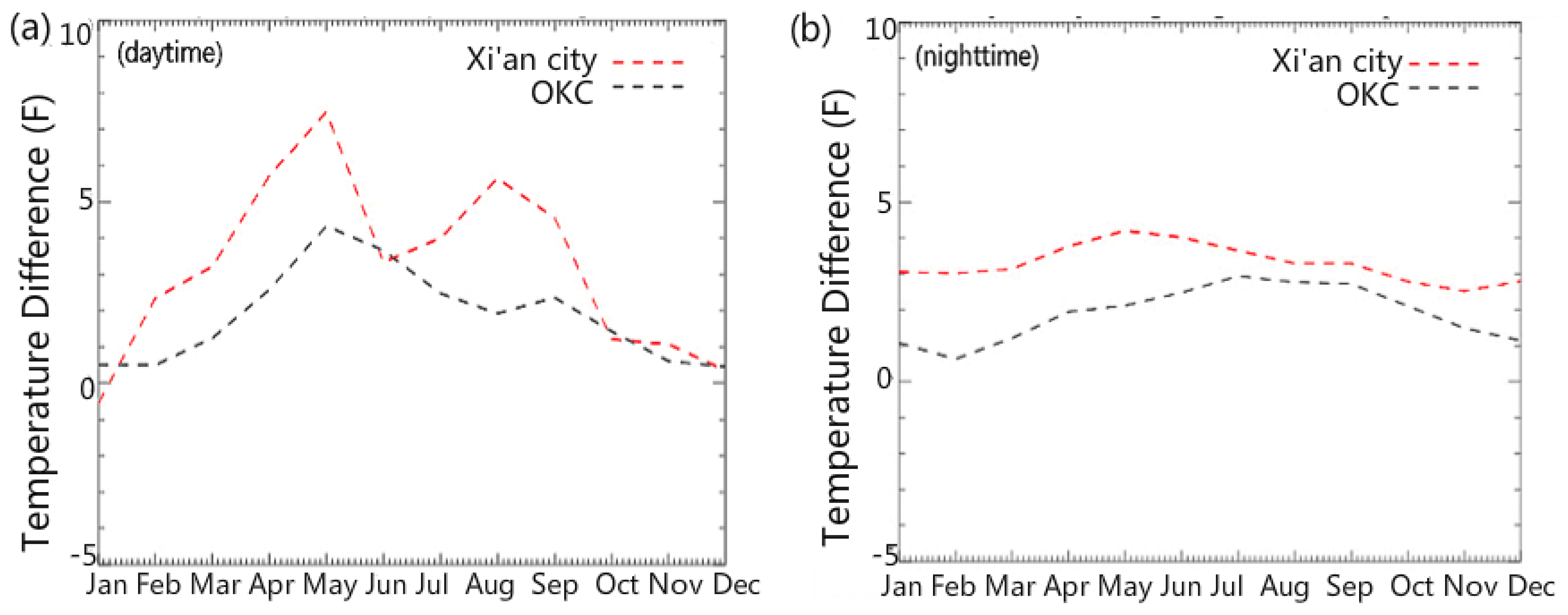
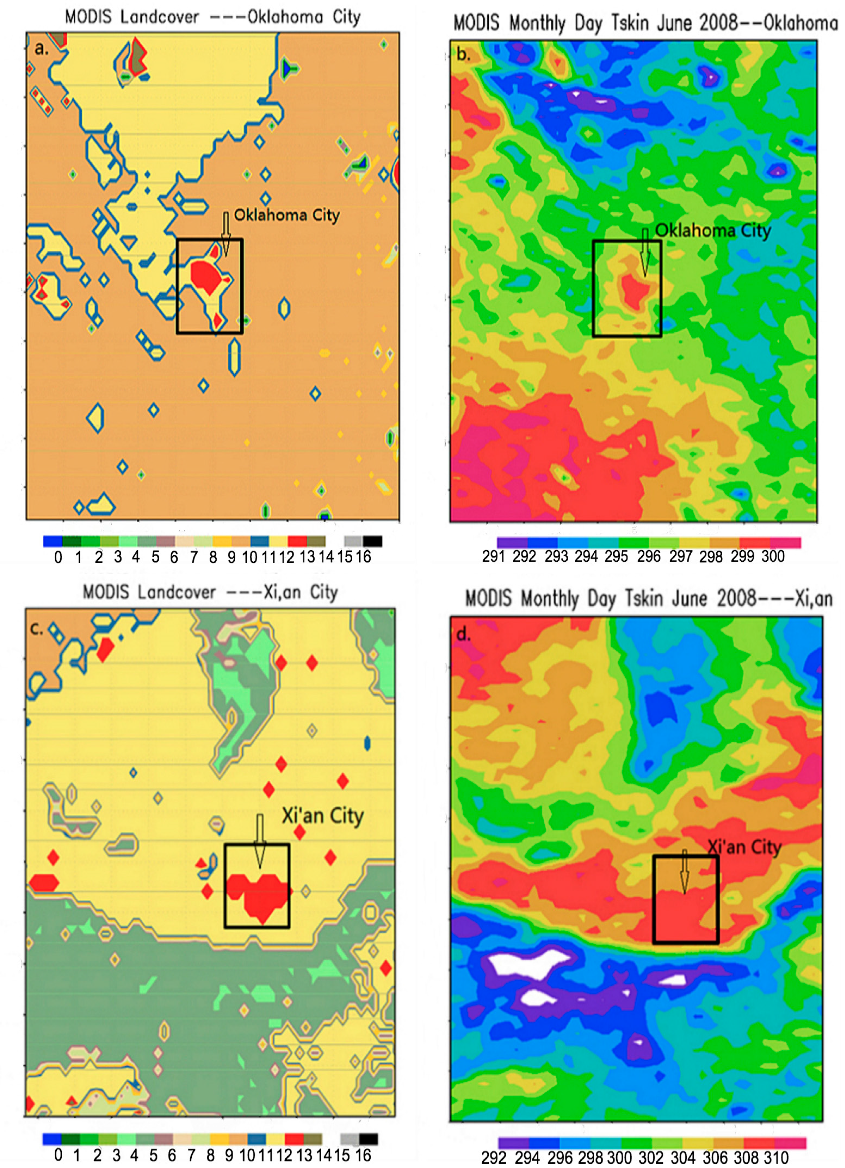
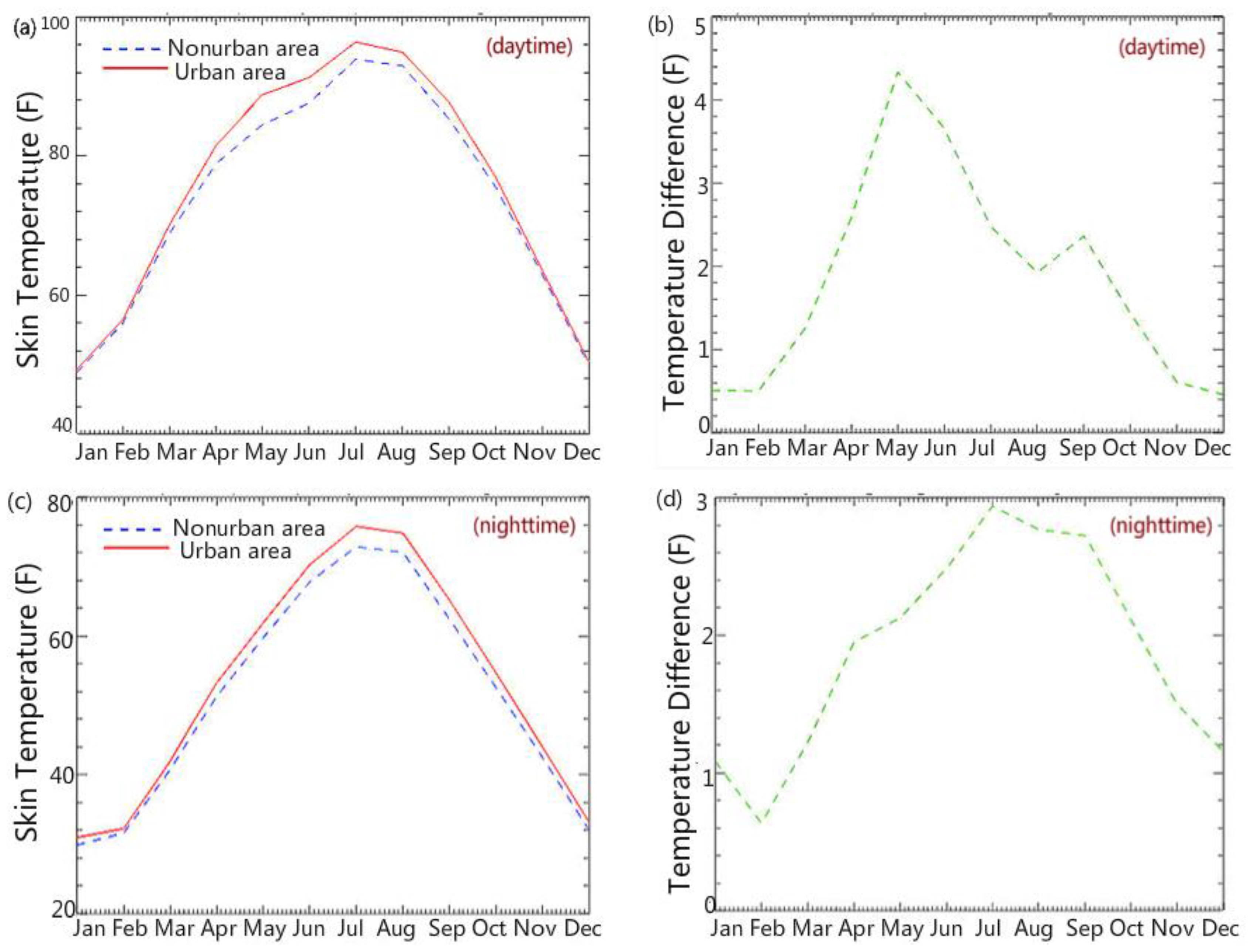
  • An urban area is a highly heterogeneous environment and different cities have different types of surrounding land covers, geometric conditions, and population densities. As a result, the UHI differs between cities such as OKC and Xi’an, although both are inland cities at the same latitude. Satellite retrieval captured the UHI for both cities. Xi’an had the stronger UHI than OKC, which suggests that the population density, building density, and city size are important factors in determining the UHI intensity.
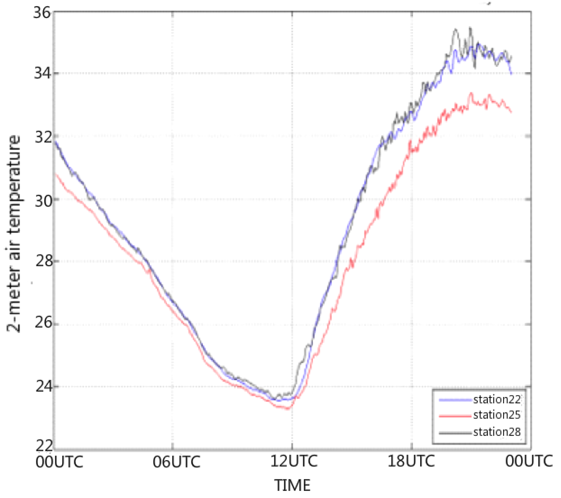
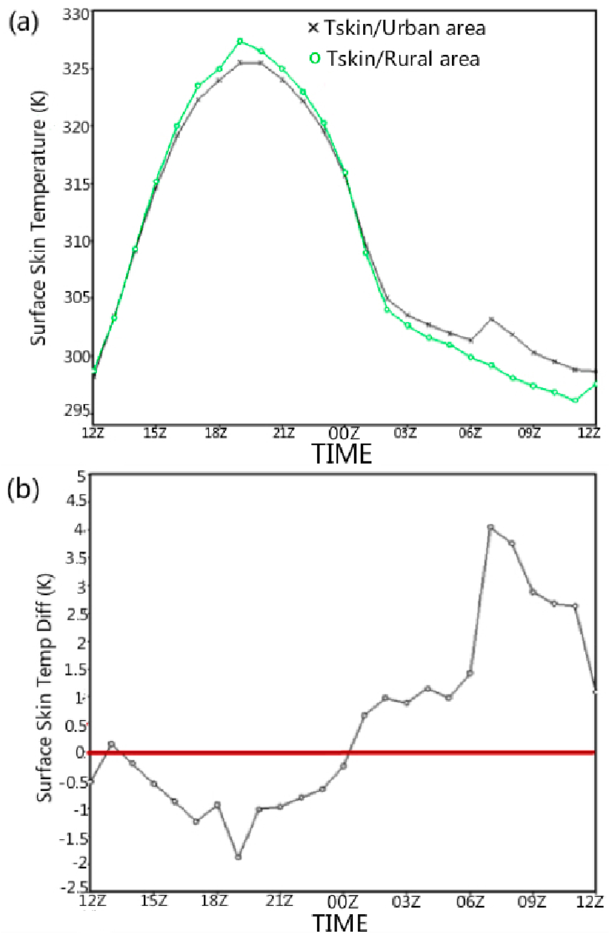
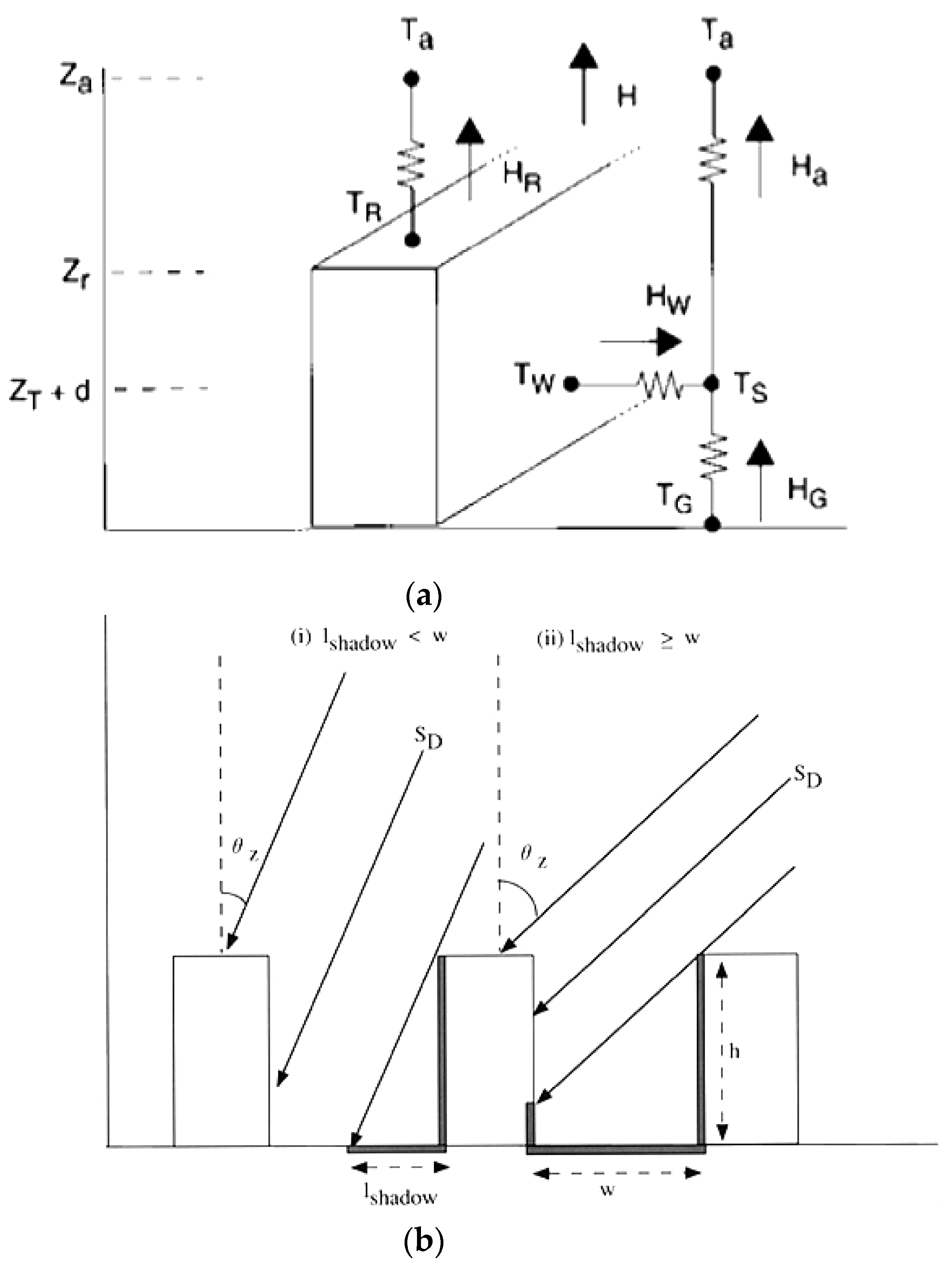
  • There are competing factors and physical processes in an urban surface-layer that make a UHI or UCI both possible. Specifically, building materials had a high heat capacity, which slowed down the warming at the surface during daytime and warmed the surface at nighttime. Furthermore, the building shadows reduced surface temperatures, as shown in ground observations, where a significant UCI occurred on summer days at noon in OKC. Nevertheless, less soil moisture and less vegetation cover over urban regions lead to a surface warming since all absorbed solar radiation was used to heat up the surface.
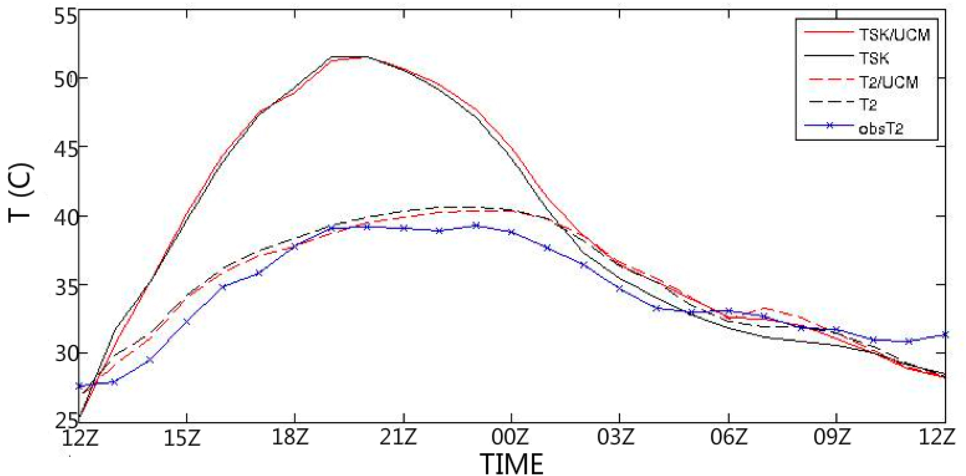
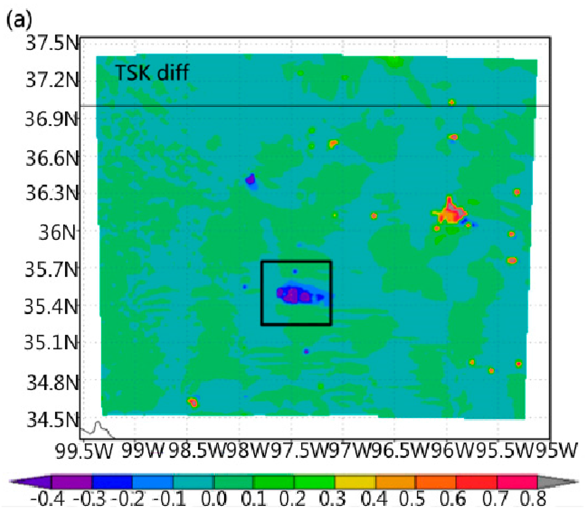
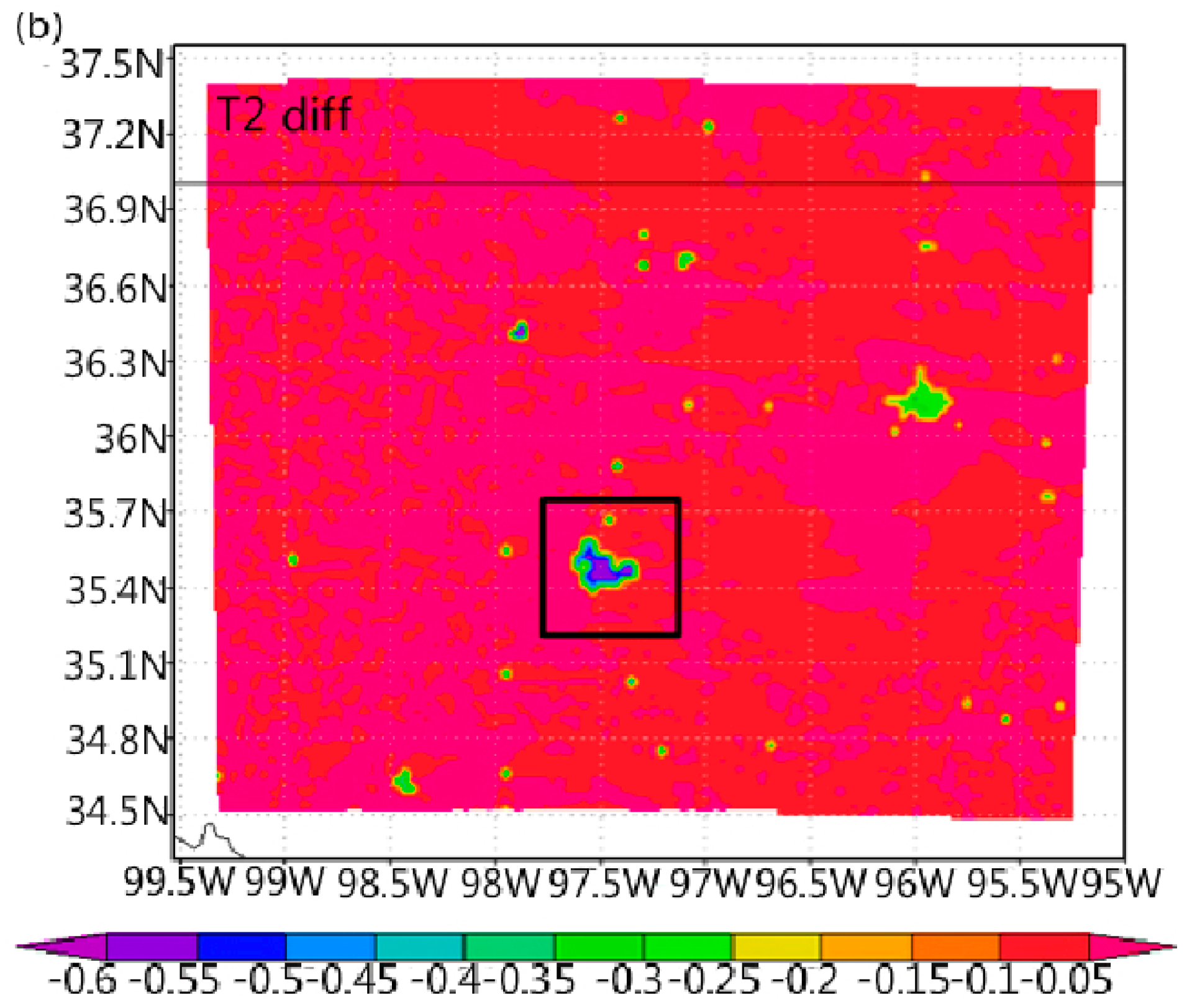
  • Skin temperature and 2 m air temperature fields may have different UHI or UCI signals. The satellite observed skin temperature in OKC, which showed an evident UHI, was monthly averaged. The ground observation of 2 m air temperature and modeled surface skin and air temperatures, which suggested a UCI, were only during daytime and at hourly resolution.
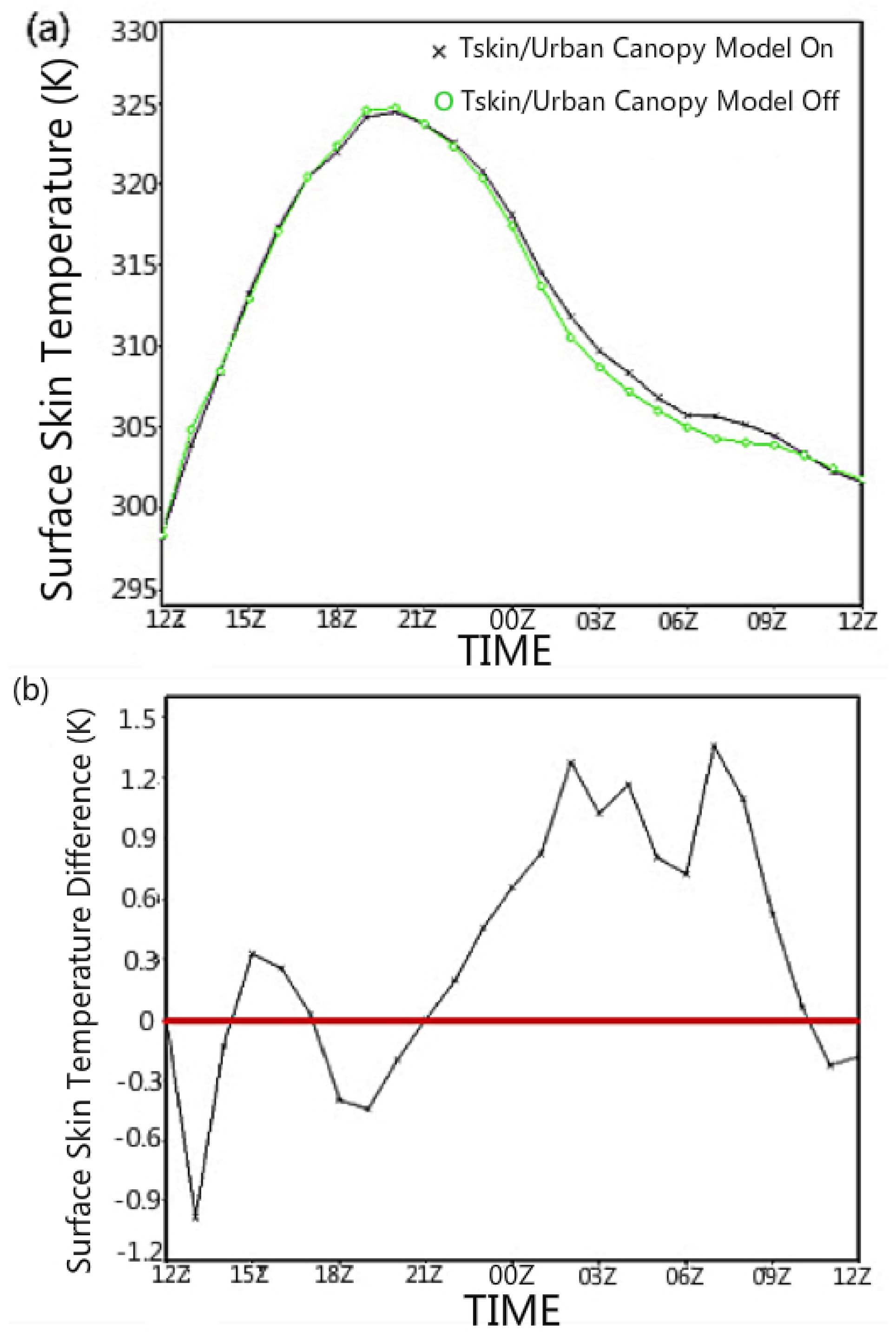
  • The coupled WRF/Noah/SLUCM modeling system can re-produce the signal of the UHI or UCI, although its intensity and duration remain problematic. Nevertheless, a main issue affecting WRF urban simulation is that the default settings in the USGS 24-category land use categories are outdated for many cities. For instance, the simulated urban fraction for OKC is only about 2%, while its actual value is about 20%, based on MODIS.
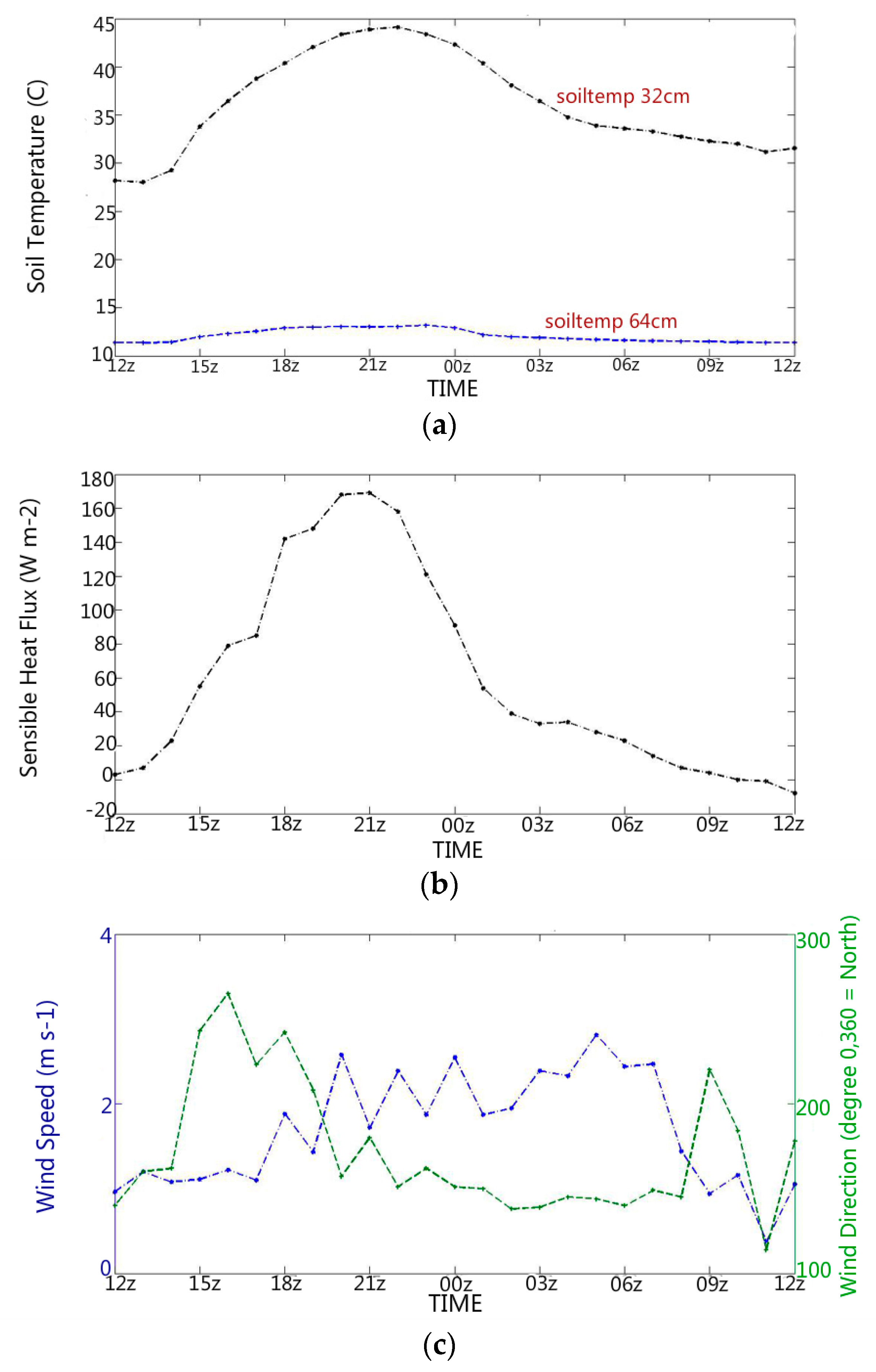
  • The coupled WRF/Noah/SLCUM model reproduces the UCI during summer daytime in OKC, which was consistent with the ground observations. However, it failed to accurately capture the influences of cities on prevalent atmospheric motions, such as wind speed, wind direction, and energy flux.
This study has a broad impact because it combined satellite observations, ground observations, and WRF model simulations, to enhance the current understanding of the UHI. In addition, both ground observations and WRF/SLUCM simulations revealed an unusual phenomenon of UCI in OKC during daytime in summer. Finally, an update of the WRF default USGS 24-category land use categories could lead to significant improvements in the quality of WRF/SLUCM simulation output, as the model urban regions for many cities are presently outdated..

Acknowledgments

This work was partly supported by NSF Large-scale Dynamics Program (Grant number 0855480) and partly supported by NASA Precipitation Program (Grant number NNX13AG99G and NX16AD87G).

Author Contributions

Leading author H. Zhang conducted the data analysis and the writing of this work. Co-author Jin supervised H. Zhang for this work, revised each version of the manuscript, and responded to the reviewer comments. Jin also finical supported this work, as a faculty, using her NSF and NASA funding. Co-author Leach run the model simulations, supervised the data analysis, and revised the manuscript in early stage.

Conflicts of Interest

The authors declare no conflicts of interest.

References

  1. Trenberth, K.T.; Fasullo, J.T.; Kiehl, J. Earth’s global energy budget. Bull. Am. Meteorol. Soc. 2009, 90, 311–323. [Google Scholar] [CrossRef]
  2. Jin, M.; Dickinson, R.E. Land surface skin temperature climatology: Benefitting from the strengths of satellite observations. Environ. Res. Lett. 2010, 5, 044004. [Google Scholar] [CrossRef]
  3. Jin, M.; Dickinson, R.E.; Vogelmann, A.M. A Comparison of CCM2/BATS Skin Temperature and Surface-Air Temperature with Satellite and Surface Observations. J. Clim. 1997, 10, 1505–1524. [Google Scholar] [CrossRef]
  4. Jin, M.; Mullens, T. Land-biosphere-atmosphere interactions over Tibetan Plateau from MODIS observations. Environ. Res. Lett. 2012, 7, 014003. [Google Scholar] [CrossRef]
  5. Landsberg, H.E. The Urban Climate; Academic Press: New York, NY, USA, 1981; 275p. [Google Scholar]
  6. Oke, T.R. The energetic basis of the Urban Heat Island. Q. J. R. Meteorol. Soc. 1982, 108, 1–24. [Google Scholar] [CrossRef]
  7. Oke, T.R. Canyon geometry and the nocturnal Urban Heat Island. Int. J. Climatol. 1981, 10, 237–245. [Google Scholar] [CrossRef]
  8. Jin, M.; Dickinson, R.E.; Zhang, D. The footprint of urban areas on global climate as characterized by MODIS. J. Clim. 2005, 18, 1551–1565. [Google Scholar] [CrossRef]
  9. Basara, J.B.; Basara, H.G.; Illston, B.G.; Crawford, K.C. The Impact of the Urban Heat Island during an Intense Heat Wave in Oklahoma City. Adv. Meteorol. 2010, 2010. [Google Scholar] [CrossRef]
  10. Jin, M.; Kessomkiat, W.; Pereira, G. Satellite-observed urbanization characters in Shanghai, China: Aerosols, urban heat island effect, and land-atmosphere interactions. Remote Sens. 2011, 3, 83–99. [Google Scholar] [CrossRef]
  11. Johansson, E.; Spangenberg, J.; Gouvêa, M.L.; Freitas, E.D. Scale-integrated atmospheric simulations to assess thermal comfort in different urban tissues in the warm humid summer of São Paulo, Brazil. Urban Clim. 2013, 6, 24–43. [Google Scholar] [CrossRef]
  12. Arnfield, A.J. Two decades of urban climate research: A review of turbulence, exchanges of energy and water, and the urban heat island. Int. J. Clim. 2003, 23, 1–26. [Google Scholar] [CrossRef]
  13. Chin, H.-N.S.; Leach, M.J.; Sugiyama, G.A.; Leone, J.M.; Walker, H.; Nasstrom, J.S.; Brown, M.J. Evaluation of an urban canopy parameterization in a mesoscale model using VTMX and URBAN 2000 data. Mon. Weather Rev. 2005, 133, 2043–2068. [Google Scholar] [CrossRef]
  14. Coutts, A.M.; Beringer, J.; Tapper, N.J. Impact of increasing urban density on local climate: Spatial and temporal variation in the surface energy balance in Melbourne, Australia. J. Appl. Meteorol. Climatol. 2007, 46, 477–493. [Google Scholar] [CrossRef]
  15. Jones, P.D.; Kelly, P.M.; Goodess, C.M. The effect of urban warming on the northern hemisphere temperature average. J. Clim. 1989, 2, 285–290. [Google Scholar] [CrossRef]
  16. Kim, Y.-H.; Baik, J.-J. Spatial and temporal structure of the urban heat island in Seoul. J. Appl. Meteorol. 2005, 44, 591–605. [Google Scholar] [CrossRef]
  17. Martilli, A. Numerical study of urban impact on boundary layer structure: Sensitivity to wind speed, urban morphology, and rural soil moisture. J. Appl. Meteorol. 2002, 41, 1247–1266. [Google Scholar] [CrossRef]
  18. Masson, V. A physically-based scheme for the urban energy budget in atmospheric models. Bound. Layer Meteorol. 2000, 94, 357–397. [Google Scholar] [CrossRef]
  19. Miao, S.; Chen, F.; LeMone, M.A.; Tewari, M.; Li, Q.; Wang, Y. An observational and modeling study of characteristics of urban heat island and boundary layer structures in Beijing. J. Appl. Meteorol. Climatol. 2009, 48, 484–501. [Google Scholar] [CrossRef]
  20. Johnson, G.T.; Steyn, D.G.; Watson, I.D. Simulation of surface Urban Heat Island. Bound. Layer Meteorol. 1991, 56, 339–358. [Google Scholar]
  21. Zeuner, G.; Jauregui, E. The surface energy balance in Mexico City. Atmos. Environ. 1992, 26, 433–444. [Google Scholar]
  22. Ren, G.; Zhou, Y.; Chu, Z.; Zhou, J.; Zhang, A.; Guo, J.; Liu, X. Urbanization effects on observed surface air temperature trends in north China. J. Clim. 2008, 21, 1333–1348. [Google Scholar] [CrossRef]
  23. Tewari, M.; Chen, F. A study of the urban boundary layer using different urban parameterizations and high-resolution urban panopy parameters with WRF. J. Appl. Meteorol. Climatol. 2011, 50, 1107–1128. [Google Scholar]
  24. Trusilova, K.; Jung, M.; Churkina, G. On climate impacts of a potential expansion of urban land in Europe. J. Appl. Meteorol. Climatol. 2009, 48, 1971–1980. [Google Scholar] [CrossRef]
  25. Montavez, J.P.; Rodriguez, A.; Jimenez, J.I. A study of the urban heat island of Granada. Int. J. Climatol. 2000, 20, 899–911. [Google Scholar] [CrossRef]
  26. Hamdi, R.; Van de Vyver, H. Estimating urban heat island effects on near-surface air temperature records of Uccle (Brussels, Belgium): An observational and modeling study. Adv. Sci. Res. 2011, 6, 27–34. [Google Scholar] [CrossRef]
  27. Yang, B. Simulation of urban climate with high-resolution WRF model: A case study in Nanjing, China. Asia Pac. J. Atmos. Sci. 2012, 48, 227–241. [Google Scholar] [CrossRef]
  28. Chen, F.; Kusaka, H.; Tewari, M.; Bao, J.-W.; Hirakuchi, H. Utilizing the Coupled WRF/LSM/Urban Modeling System with Detailed Urban Classification to Simulate the Urban Heat Island Phenomena over the Greater Houston Area. In Proceedings of the Fifth Symposium on the Urban Environment, Vancouver, BC, Canada, 22–27 August 2004. [Google Scholar]
  29. Salamanca, F.; Krpo, A.; Martilli, A.; Clappier, A. A new building energy model coupled with an urban canopy parameterization for urban climate simulations—Part I. Formulation, verification, and sensitivity analysis of the model. Theor. Appl. Climatol. 2010, 99, 331. [Google Scholar] [CrossRef]
  30. Garratt, J.R. The Atmospheric Boundary Layer; Cambridge University Press: Cambridge, UK, 1992; p. 315. [Google Scholar]
  31. Janković, V.; Hebbert, M. Hidden climate change–urban meteorology and the scales of real weather. Clim. Chang. 2012, 113, 23–33. [Google Scholar] [CrossRef]
  32. Jin, M.; Shepherd, J.M. Aerosol relationships to warm season clouds and rainfall at monthly scales over east China: Urban land versus ocean. J. Geophys. Res. 2008, 113, D24S90. [Google Scholar] [CrossRef]
  33. Allwine, K.J.; Flaherty, J.E. Joint Urban 2003: Study Overview and Instrument Locations; Pacific Northwest National Laboratory (PNNL): Richland, WA, USA, 2006; p. 15967.
  34. Kusaka, H.; Kondo, H.; Kikegawa, Y.; Kimura, F. A simple single-layer urban canopy model for atmospheric models: Comparison with multi-layer and slab models. Bound. Layer Meteorol. 2001, 101, 329–358. [Google Scholar] [CrossRef]
  35. Chen, F.; Kusaka, H.; Bornstein, R. The integrated WRF/urban modeling system: Development, evaluation, and applications to urban environmental problems. Int. J. Climatol. 2011, 31, 273–288. [Google Scholar] [CrossRef]
  36. King, M.D.; Menzel, W.P.; Kaufman, Y.J.; Tanre, D.; Gao, B.-C.; Platnick, S.; Ackerman, S.A.; Remer, L.A.; Pincus, R.; Hubanks, P.A. Cloud and aerosol properties, precipitable water, and profiles of temperature and humidity from MODIS. IEEE Trans. Geosci. Remote Sens. 2003, 41, 442–458. [Google Scholar] [CrossRef]
Figure 1. (a) Overview of the PNNL Meteorological Station and HOBO locations. The light green pentagons are HOBOs, while the dark green pentagons are meteorological stations (33, ©Courtesy of Battelle memorial Institute. From the Pacific Northwest National Laboratory for the U.S. Department of Energy; (b) Overview of the Atmospheric Turbulence and Diffusion Division (ATDD) flux site locations (Hanna 2011, personal communication). These maps cover Oklahoma City.
Climate 05 00072 g001aClimate 05 00072 g001b
Figure 2. Schematic illustration of the Single-Layer Urban Canopy Model, (a) showing transfers of heat among objects in the model. Ta: air temperature at reference height Za. TR: building roof temperature. TW: building wall temperature. TG: road temperature. TS: temp defined at ZT + d. H: sensible heat exchange at reference height. Ha: sensible heat flux from the canyon space to atmosphere. HW: sensible heat flux from wall to canyon space. HG: sensible heat flux from road to canyon space. HR: sensible heat flux from roof to the atmosphere; (b) Radiation of the single-layer urban canopy model. SD: direct solar radiation on a horizontal surface. w: normalized road width. h: normalized building height. w + r = 1, where r is the normalized roof width. lshadow: normalized shadow length on the road. θz: solar zenith angle. Kusaka et al. [34], ©Springer.
Climate 05 00072 g002
Figure 3. Three nesting domains with 25, 5, and 1 km grid spacing in WRF simulation.
Climate 05 00072 g003
Figure 4. MODIS land surface cover type of (a) Oklahoma and (c) Xi’an. MODIS classifies the land cover to 17 differing classifications: (1) Evergreen Needleleaf Forest, (2) Evergreen Broadleaf Forest, (3) Deciduous Needleleaf Forest, (4) Deciduous Broadleaf Forest, (5) Mixed Forest, (6) Closed Shrubland, (7) Open Shrubland, (8) Woody Savannas, (9) Savannas, (10) Grassland, (11) Permanent Wetland, (12) Cropland, (13) Urban and Built-up, (14) Cropland/Natural Vegetation Mosaic, (15) Snow and Ice, (16) Barren or Sparsely Vegetated. Urban area is the red color in the mapped areas. Locations of OKC and Xi’an City are marked in the figures. MODIS monthly daytime land surface skin temperature (unit in K) was recorded in June 2008 by Terra at 10:30 local time for (b) OKC in June 2008 and (d) Xi’an City.
Climate 05 00072 g004
Figure 5. (a) OKC monthly averaged daytime skin temperature (2001–2008); (b) OKC monthly averaged daytime skin temperature difference (urban–nonurban); (c) OKC monthly averaged nighttime skin temperature (2001–2008); (d) OKC monthly averaged nighttime skin temperature difference (urban–nonurban). Temperature unit in °F.
Climate 05 00072 g005
Figure 6. (a) Xi’an City and OKC monthly averaged daytime skin temperature difference (urban–nonurban); (b) Xi’an City and OKC monthly averaged nighttime skin temperature difference (urban–nonurban). Temperature unit in °F.
Climate 05 00072 g006
Figure 7. The temperature difference (e.g., Delta T, unit in °C) values for 2 m air temperatures for each station in (a) the x-direction and (b) the y-direction.
Climate 05 00072 g007
Figure 8. 24 h diurnal variation of 2 m air temperatures (unit in °C) from PNNL HOBO Station No. 22, Station No. 25, and Station No. 28.
Climate 05 00072 g008
Figure 9. Map of locations of the PNNL HOBO Station No. 22, Station No. 25, and Station No. 28. This map covers Oklahoma City.
Climate 05 00072 g009
Figure 10. (a) ATDD Flux Site C observed 24 h diurnal variation of soil temperature (unit in °C) at 32 cm and 64 cm in OKC; (b) ATDD Flux Site C observed 24 h diurnal variation of sensible heat flux (W/m2) in OKC; (c) ATDD Flux Site C observed 24 h diurnal variation of wind speed (unit in m/s) and wind direction in OKC.
Climate 05 00072 g010
Figure 11. (a) WRF simulated surface temperature difference at 18:00 UTC, 19 July 2003, in OKC for the Tskin difference (sensitive run–control run); (b) WRF simulated surface temperature difference at 18:00 UTC, 19 July 2003, in OKC for a 2 m Tair difference (sensitive run–control run). Temperature unit is in K; OKC is highlighted by the rectangle.
Climate 05 00072 g011aClimate 05 00072 g011b
Figure 12. (a) The WRF model simulated skin temperature (Tskin) for the sensitive run and control run in urban regions in OKC. The green curve is for the control run (i.e., Tskin with urban canopy model off in the WRF simulation), and the black curve is for the simulation of the sensitive run (i.e., Tskin with urban canopy model turned on in WRF simulation); (b) Skin temperature difference between the sensitive run and control run (sensitive run minus control run) in urban regions in OKC. Temperature and temperature difference are in K.
Climate 05 00072 g012
Figure 13. (a) The WRF/SLUCM-simulated Tskin (urban vs. rural) in OKC, with the green curve representing the Tskin over the OKC urban area, and the black curve representing the Tskin over its rural area; (b) The SLUCM-simulated Tskin difference (urban–rural) in OKC. Temperature and temperature difference is in K.
Climate 05 00072 g013
Figure 14. Comparison of WRF-simulated skin temperature (TSK in legend) and 2 m air temperature (e.g., T2) with the ground-observed air temperature (e.g., obs T2). The red solid line represents the model-simulated skin temperature with SLUCM turned on (e.g., the sensitive run); the black solid line represents the model-simulated skin temperature without SLUCM turned on (e.g., the control run); the red dashed line shows the model-simulated 2 m air temperature with SLUCM; the black dashed line shows the model-simulated 2 m air temperature without SLUCM; the blue line represents the ground-observed air-temperature from PNNL HOBO Station 9. Temperature is in °C.
Climate 05 00072 g014
Figure 15. (a) The WRF-simulated downward shortwave radiation and ground-observed downward shortwave radiation in OKC; (b) The WRF-simulated net radiation and ground-observed net radiation in OKC.
Climate 05 00072 g015
Table 1. Surface parameters, canyon dimensions, and physical constants used in WRF runs (credit to WRF user’s manual).
ParameterSymbolValueUnit
Roof level (building height)zr15[m]
Normalized building heighth0.5
Normalized roof widthr0.25
Normalized road widthw0.75
Urban area ratio for a gridAu
Vegetation area ratio for a gridAv0
Roughness length for momentum above cityZ0m0.5[m]
Roughness length for momentum above canyonZ00.667[m]
Roughness length above roofzoR0.005[m]
Zero plane displacement heightd2.3[m]
Roof surface albedoαR0.2
Wall surface albedoαW0.2
Road surface albedoαG0.2
Roof surface emissivityϵR0.97
Wall surface emissivityϵW0.97
Road surface emissivityϵG0.97
Canyon orientationθcan/8 (n = 0 − 7)[rad]
Physical ConstantSymbolValueUnit
Volumetric heat capacity of roofρRCR2.01 × 106[J m−3 K−1]
Volumetric heat capacity of wallρWCW2.01 × 106[J m−3 K−1]
Volumetric heat capacity of roadρGCG2.01 × 106[J m−3 K−1]
Thermal conductivity of roofλR2.28[W m−1 K−1]
Thermal conductivity of wallλW2.28[W m−1 K−1]
Thermal conductivity of roadλG2.28[W m−1 K−1]

