Decreasing Past and Mid-Century Rainfall Indices over the Ouémé River Basin, Benin (West Africa)

Abstract

This study analyzed the trends of extreme daily rainfall indices over the Ouémé basin using the observed data from 1950 to 2014 and the projected rainfall of regional climate model REMO (REgional MOdel) for the period 2015–2050. For future trends analysis, two Intergovernmental Panel on Climate Change (IPCC) new scenarios are considered, namely RCP4.5 and RCP8.5. The indices considered are number of heavy rainfall days, number of very heavy rainfall days, consecutive dry days, consecutive wet days, daily maximum rainfall, five-day maximum rainfall, annual wet-day total rainfall, simple daily intensity index, very wet days, and extremely wet days. These indices were calculated at annual and seasonal scales. The Mann-Kendall non-parametric test and the parametric linear regression approach were used for trends detection. As result, significant declining in the number of heavy and very heavy rainfall days, heavy and extremely heavy rainfall, consecutive wet days and annual wet-day rainfall total were detected in most stations for the historical period as well as the future period following the scenario RCP8.5. Furthermore, few stations presented significant trends for the scenario RCP4.5 and the high proportion of stations with the inconsistence trends invites the planners to get ready for an uncertain future climate following this scenario.

1. Introduction

Uncertainties on future availability of water resources and extremes events are the most important issue that water management planners are facing. To this end, understanding trends and variations of historical and future climatic variables is pertinent for the future development and sustainable water resources management in a given region [1]. Therefore, one of the very important necessities of research into climate change is to analyse and detect historical changes in the climatic system [2,3]. Since rainfall is a principal element of the hydrological cycle, understanding its behaviour may be of profound social and economic significance [4]. Within this context, the detection of trends of extreme rainfall in long-term observational records and climate projections yields important information for the understanding of climate change and its impact on crucial sectors such as agriculture, ecosystems and water resources.

Most existing studies from around the world indicate a positive trend in the daily precipitation intensity and a tendency toward higher frequencies of heavy and extreme rainfall in the last few decades. Indeed, significant positive trends have been observed in the USA [5,6], East and Northeast Australia [7], Chinas coastal area [8], Germany [9], India [10], France [11], eastern and western Indochina Peninsula [12]. However, there are negative trends in extreme rainfall events reported for some regions like Poland [13].

For Africa, changes in extreme precipitation are contrasted. In the northern part of Africa, there is a tendency towards wetter conditions; in contrast with the eastern part, experienced with more drying trends, although, these trends are of low significance [14]. In sub-Saharan Africa, some studies indicated an increase in extreme rainfall events, particularly in western Niger [15] but also a decrease in Nigeria [4,16], Guinea Conakry [17], in eastern Niger [18], Ivory-Coast [19] and in South Africa [20].

It should be noted that studies on extreme climate events have been conducted in most regions over the world, which typically were preceded by workshops coordinated by the Expert Team on Climate Change Detection and Indices (ETCCDI) [12,14]. Nevertheless, there is a paucity of information on trends in daily extreme rainfall events regarding the African continent, especially in West Africa [3]. This is mainly due to several reasons including the scarcity and poor quality of daily observational data in this region and also because several countries have restrictive policies on data sharing [14,19].

For the specific case of Benin, few studies were devoted to climate indices analysis. Hountondji et al. [21] studied trends in extreme rainfall events in Benin for the period 1960–2000 using 21 rainfall stations. They indicated significant decreasing trends only for the annual total precipitation, the annual total of wet days and the annual maximum rainfall while the other rainfall indicators such as the simple day intensity index, the number of very wet day and the extreme rainfall frequency, appear to remain stable. Even though an effort has been made in [21], 15 years after the end year considered (2000), it is necessary to evaluate the new trends of climate indices using the recent World Meteorological Organization (WMO) reference period 1981–2010. Hounkpè et al. [22] conducted a study devoted to changes in heavy rainfall characteristics over the Ouémé River Basin (Benin). The main finding is the positive change associated with an increase in heavy rainfall over the area of concern. This study analyzed well the heavy historical precipitation for the period 1960–2012 but based on the uncommon climate indices used in impact studies. Indeed, the thresholds established by WMO to define extreme rainfall are of relevance to particular applications such as flood and drought early warning systems contrary to the three thresholds used in [22]. These two studies devoted to climate indices in Benin didn’t prospect the future trends of the precipitations index nevertheless pertinent for the future development and sustainable management of water resources.

Despite these efforts to study extreme rainfall, there is a real gap on past and future rainfall indices trends analysis based on the climate indices such as defined by the World Meteorological Organization. The present study has been conducted in the intent to fill this gap, by examining trends of past and future rainfall indices in Ouémé basin in Benin.

2. Materials and Methods

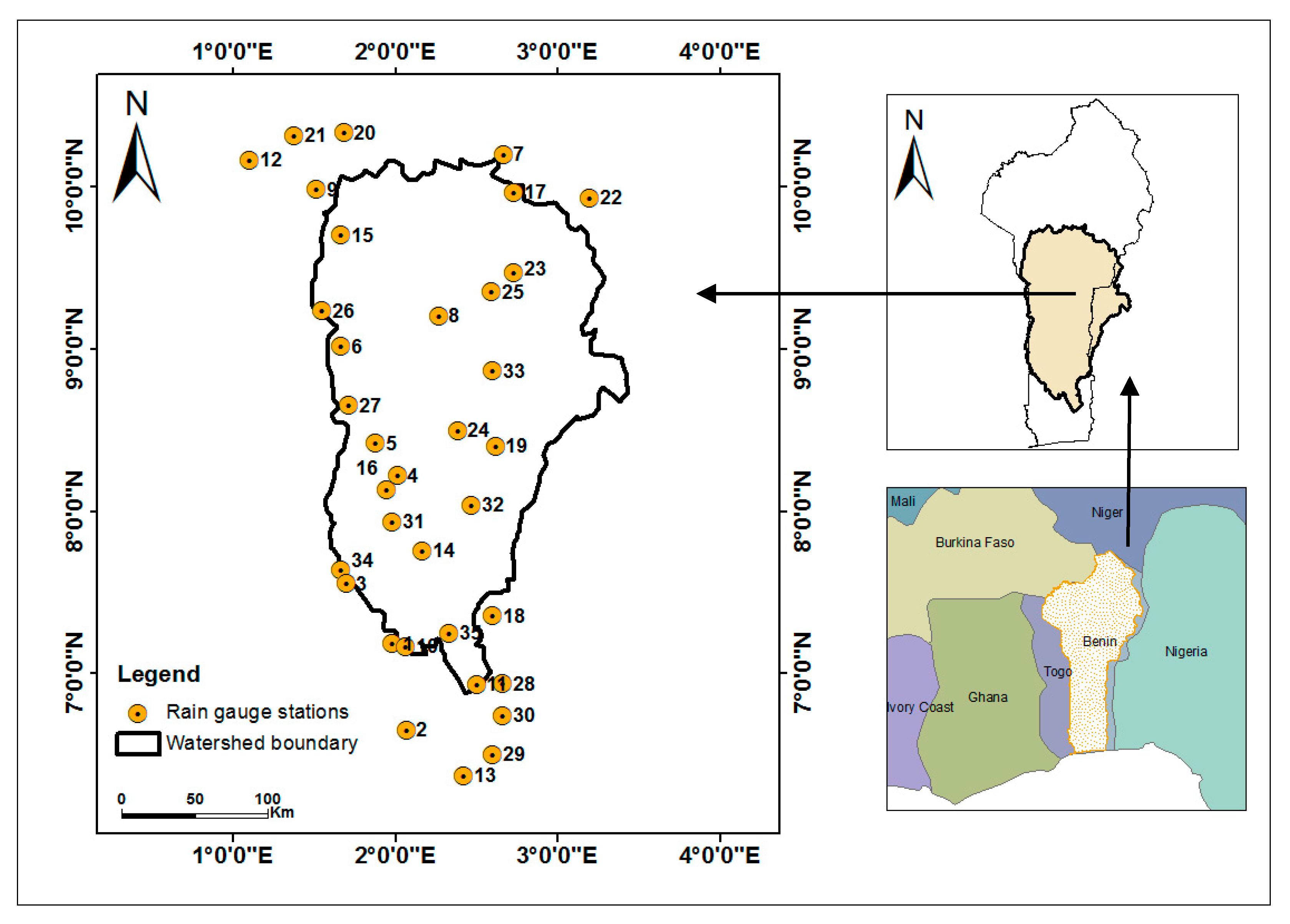
2.1. Study Area

The present study focuses on Ouémé river basin at the outlet of Bonou (Figure 1). This basin is located between the latitudes 7°58′ North to 10°12′ North and longitudes 1°30′ East to 3°05′ East and covers an area of 49,256 km². In general, West Africa’s climate is controlled by the interaction of two air masses, the influence of which varies throughout the year with the north-south movement of the Intertropical Convergence Zone (ITCZ). Hot, dry continental air masses originating from the high pressure system above the Sahara desert give rise to dusty Harmattan winds over most of West Africa from November to February. In summer, moist equatorial air masses originating over the Atlantic Ocean bring annual monsoon rains [23]. Within this West African context, rainfall in the study area is characterized by two types of rainfall regimes. In southern there are two rainy seasons which extend from mid-March to mid-July and from mid-August to October. In northern basin, there is one rainy season extends from April to October. The average discharge of the main watercourse of this basin is approximately 50 m³/s at Bétérou hydrometric station from 1960 to 2013 and 190.75 m³/s at Bonou station for the same period. The annual rainfall average is 1200 mm/year from 1960 to 2014.

2.2. Datasets

Two types of data were used in this study. The first one constitutes the daily rainfall data from thirty five stations (Figure 1) available for the period 1950–2014; these data were obtained from the National Meteorology Agency of Benin (Météo Bénin). The spatial distribution is showed in Figure 1.

The missing rate is calculated over the whole recording period, ending in 2014. This rate is more important for some stations exploited since 1921 (

Table 1. List of selected rainfall gauge stations used.

No.	Stations Name	Long. (deg.)	Lat. (deg.)	Creation Year	Missing Rate (%)	No.	Stations Name	Long. (deg.)	Lat. (deg.)	Creation Year	Missing Rate (%)
1	Abomey	1.98	7.18	1921	2.0	19	Kokoro	2.62	8.40	1969	5.0
2	Adjohoun	2.48	6.70	1921	3.3	20	Kouandé	1.68	10.33	1931	4.0
3	Agouna	1.70	7.55	1968	12.0	21	Natitingou	1.38	10.32	1921	0.0
4	Aklampa	2.02	8.55	1968	4.0	22	Nikki	3.20	9.93	1921	10.0
5	Bantè	1.88	8.42	1942	8.0	23	Okpara	2.73	9.47	1956	4.0
6	Bassila	1.67	9.02	1950	12.0	24	Ouèssè	2.60	8.67	1964	1.4
7	Bembèrèkè	2.67	10.20	1921	0.0	25	Parakou	2.60	9.35	1921	1.0
8	Bétérou	2.27	9.20	1953	7.0	26	Pénéssoulou	1.55	9.23	1969	20.0
9	Birni	1.52	9.98	1953	10.0	27	Pira	1.72	8.65	1968	6.0
10	Bohicon	2.07	7.17	1940	0.2	28	Pobè	2.67	6.93	1926	7.0
11	Bonou	2.50	6.93	1946	7.0	29	Porto-Novo	2.61	6.48	1921	3.0
12	Boukombé	1.10	10.16	1952	11.0	30	Sakété	2.07	6.72	1921	10.0
13	Cotonou	2.38	6.35	1921	0.0	31	Savalou	1.98	7.93	1921	17.0
14	Dassa-Zoumè	2.17	7.75	1941	0.0	32	Savè	2.47	8.03	1921	16.0
15	Djougou	1.67	9.70	1921	5.0	33	Tchaourou	2.60	8.87	1937	13.0
16	Gouka	1.95	8.13	1968	6.0	34	Tchetti	1.67	7.82	1964	17.0
17	Ina	2.73	9.97	1947	6.0	35	Zagnanando	2.33	7.25	1921	0.1
18	Kétou	2.60	7.35	1950	5.0

). The missing data are more present before 1950. So we have considered for analysis, 1950–2014. For data processing, any year which contains more than 10% missing values between April and October (rainy period) is considered like missing and the climate indices aren’t calculated for this year.

The second type of data used constitutes the daily rainfall data from a set of simulations (scenario) conducted with the regional climate model REMO. REMO is a three-dimensional, hydrostatic atmospheric circulation model which solves the discretized primitive equations of atmospheric motion. The REMO simulations are forced with data from the global climate model MPI-ESM-LR following the IPCC (Intergovernmental Panel on Climate Change) Representative Concentration Pathways (RCP) scenarios. The details of the model characteristics are summarized in

Table 2. REMO model characteristics.

Institute	Climate Service Centre, Hamburg, Germany
Main driving Model	MPI-ESM-LR
Projection	Rotated spherical grid
Resolution	0.44 degree
Vertical coordinates	Hybrid
Vertical levels	27
Advection	Semi-lagrangian
Time step	240 s
Convection Scheme	Tiedke [24]
Radiation Scheme	Morcrette et al. [25]; Giorgetta and Wild [26]
Turbulence vertical diffusion	Louis [27]
Cloud Microphysics Scheme	Lohmann and Roeckner [28]
Land Surface Scheme	Hagemann [29]; Rechid et al. [30]

Further details about REMO model can be found in [31].

.

REMO data are available in the context of the Coordinated Regional Climate Downscaling Experiment (CORDEX) over Africa at 0.44° resolution for the period 1950 to 2100 [32] and it has already been used over Africa by [33,34,35,36] and particularly in Benin by [37]. Simulated precipitation of ten (10) regional climate models was evaluated at a range of time scales including seasonal means, annual and diurnal cycles, against a number of detailed observational datasets by [38]. According to their analysis, REMO produce good simulations of precipitation over West Africa. Furthermore, N’Tcha M’Po et al. [39] have compared four regional climate models ability to reproduce the daily precipitation characteristics, after bias correction, in the Ouémé watershed which is the study area of this paper. They confirmed REMO high capacity to reproduce daily precipitation in this area compared to the three others. In addition, the comparison of simulated and measured rainfall amounts in Benin has shown that REMO is able to compute realistic precipitation amounts for the region [40]. Then the choice of this model is based on prior results obtained by [38].

We used REMO projections following the most extreme IPCC scenario RCP8.5 and the mean RCP4.5 for the period 2015–2050 in CORDEX database. We also used REMO historical data from 1973 to 2005 for bias correction. All these data are available in the CORDEX database online [41].

Several researchers demonstrated that raw output from regional climate models (RCMs) cannot be used directly as input for impact models because of systematic bias [34,36,39,42,43]. Before the future precipitation index was calculated, we corrected the bias of the raw output of the RCM with a new quantile—quantile calibration method based on a nonparametric function that amends mean, variability, and shape errors in the simulated cumulative distribution functions (CDFs) of the climatic variables, developed by [44]. Indeed, two studies devoted to the comparison of daily precipitation bias correction methods were done in Benin namely N’Tcha M’Po et al. [39] and Obada et al. [45]. In these studies, six daily precipitation bias correction methods were compared and the new quantile method (AQM: Adjusted Quantile Mapping) is the most adapted method to reduce the bias of the daily precipitation simulated by the RCMs in Benin. The procedure consists of calculating the changes, quantile by quantile, in the CDFs of daily RCM outputs between a x-year control period and successive x-year future time slices [39,44]. These changes are rescaled based on the observed CDF for the same control period, and then added, quantile by quantile, to these observations to obtain new calibrated future CDFs that convey the climate change signal [44]. The choice of x value depends on the length of the observation datasets available; but the x-year chosen must have a climatological meaning [44]. In this study, we chose the 15-year periods due to the temporal limitation of the observed database of reference period (33 years, 1973–2005) and also to be in accordance with N’Tcha M’Po et al. [39] since it is the same stations. Furthermore, we consider a length of 15 years to be a compromise between series large enough to have climatological meaning; here the statistical sample is N = 5478, and short enough to permit, by comparing the simulated CDFs (Cumulative Distribution Functions) of successive 15-year to detect any climate change signal along the twenty-first century. Reference period is the period for which both observed and historical simulations of REMO data are available. We have calibrated the method over 15-year periods chosen between 1973 and 1990 and the period 1991–2005 is used to test model in order to assess the effect of calibration period on model performance. In short we have four (4) 15-year calibration periods in the period 1973–1990 (1973–1987, 1974–1988, 1975–1989 and 1976–1990), one 15-year period contains 15 consecutive years. Based on the model efficiency on different calibration periods, we chose 1976–1990 as baseline period for the correction of projected data. The best efficiency of model is obtained on the nearest period (1976–1990) to validation period (1991–2005).

Recalling that, our reference period extends from 1976 to 1990 and the future periods are 2015–2029 and 2030–2050. The statistical adjustment can be written as the following relationship between the ith percentile value $P_i$ (projected or future corrected), $O_i$ (reference observed), $S_{ci}$ (raw reference simulated), and $S_{fi}$ (raw future simulated) of the corresponding CDFs. This is just a summary of the method, all details can be found in [44].

$$P_i=O_i+g\overline{\mathrm{\Delta }}+f\mathrm{\Delta }{\prime }_i$$

(1)

With

$${\mathrm{\Delta }}_i=S_{fi}-S_{ci}$$

(2)

$$\overline{\mathrm{\Delta }}=\frac{1}{N}{\displaystyle \sum _{i=1}^N{\mathrm{\Delta }}_i}=\overline{S_f}-\overline{S_c}$$

(3)

$$\mathrm{\Delta }{\prime }_i={\mathrm{\Delta }}_i-\overline{\mathrm{\Delta }}$$

(4)

$$g=\frac{\frac{1}{N}\left({\displaystyle \sum _{i=1}^N{O}_i}\right)}{\frac{1}{N}\left({\displaystyle \sum _{i=1}^N{S}_{ci}}\right)}=\frac{\overline{O}}{\overline{S_c}}$$

(5)

and

$$f=\frac{\overline{O}}{\overline{S_c}}=\frac{IQ{R}_{|O}}{IQ{R}_{|S_c}}$$

(6)

As surrogates of the population variability, Amengual et al. [44] proposed $IQ{R}_{|O}$ (interquartile range of the observed data) and $IQ{R}_{|Sc}$ (interquartile range of the raw control simulated data). $IQR$ is the parametric difference between the 75th and 25th percentiles for all the variables, except for the precipitation for which they proposed to use 90th and 10th percentiles owing to the highly asymmetrical gamma-type distribution of this variable, with a high proportion of no-rainy days. Factor $g$ modulates the variation in the mean state $\overline{\mathrm{\Delta }}$, while $f$ calibrates the change in variability and shape expressed by $\mathrm{\Delta }{\prime }_i$.

A difficulty arises for precipitation since the climate model overestimates the number of days resulting in trace values and so underestimates the number of non-rainy days, thus resulting in an unrealistic probability of precipitation in the simulations [38,46]. To overcome this problem while respecting the internal dynamical evolution of the modeled climate scenario when dealing with the drying or moistening of the rainfall regimes and according to [44], we imposed an additional constraint: the ratio of non-rainy days between future and control simulated raw data is maintained for the calibrated versus observed series, which is $n{z}_p=\frac{n{z}_{S_f}}{n{z}_{Sc}}n{z}_O$ with $n{z}_p$, $n{z}_o$, $n{z}_{S_c}$ and $n{z}_{S_f}$ are the number of zeros in the projected, observed, simulated reference, and simulated future series, respectively.

All details about this bias correction method can be found in [39,44,45]. The MeteoLab toolbox is used to compute REMO data. MeteoLab is an open source MATLAB toolbox for meteorology and climate. It is available on http://meteo.unican.es/en/meteolab.

2.3. Extreme Precipitation Indices

Several indicators have been established by the Expert Team on Climate Change Detection Monitoring Indices (ETCCDMI) for understanding climate extremes and trends in several regions [14,19,47,48,49]. In this study, eleven extreme precipitation indices defined by ETCCDMI were analyzed. Some of them are based on fixed thresholds that are the same for all stations in these cases. These thresholds are of relevance to particular applications such as flood early warning systems. Other indices depend on the thresholds which are typically defined as a percentile of the relevant data series. In these cases the thresholds vary from location to location. The details of the indices are presented in

Table 3. List of the extreme precipitation indices used in this study.

ID	Indicator Name	Definitions	Units
RX1day	Max 1-day precipitation amount	Annual maximum 1-day precipitation	mm
RX5day	Max 5-day precipitation amount	Annual maximum consecutive 5-day precipitation	mm
SDII	Simple daily intensity index	Annual total precipitation divided by the number of wet days (defined as PRCP ≥1 mm) in the year	mm/day
R10mm	Number of heavy precipitation days	Annual count of days when PRCP ≥10 mm	days
R20mm	Number of very heavy precipitation days	Annual count of days when PRCP ≥20 mm	days
R1mm	Number of days wet days	Annual count of days when PRCP ≥1 mm	days
CDD	Consecutive dry days	Maximum number of consecutive days with PRCP <1 mm	days
CWD	Consecutive wet days	Maximum number of consecutive days with PRCP ≥1 mm	days
R95pSUM	Very wet days	Annual total precipitation when PRCP >95th percentile of period 1981–2010	mm
R99pSUM	Extremely wet days	Annual total precipitation when PRCP >99th percentile of period 1981–2010	mm
PRCPTOT	Annual total wet-day precipitation	Annual total precipitation in wet days (PRCP ≥ 1 mm)	mm

PRCP = daily total precipitation.

. As summarized in Table 3, daily extreme precipitation indices are based on relative thresholds. 95th and 99th percentiles values of WMO current reference period 1981–2010 were used to calculate the accumulation of wet and extremely wet days precipitation respectively. Single day precipitation total maximum were considered (RX1day), and cumulative values for consecutive days at individual weather sites were used to define annual maximum five-day precipitation (RX5day). Consecutive dry (CDD) and wet (CWD) days were used to examine durational characteristics of extreme precipitation events. Extreme precipitation events exceeding absolute thresholds of precipitation are characterized by the number of days with precipitation exceeding 10 mm (R10mm), 20 mm (R20mm).

2.4. Temporal Trend Analysis

Many techniques can be used for analysing the series trends, yet the most commonly used technique by meteorologists is the Mann-Kendall (MK) test [3,12,19,21,48,49]. There are two advantages of using this test. The Mann-Kendall test is non-parametric, does not require normally distributed data, and has a low sensitivity to missing data [12]. This method has also an advantage to have a low sensitivity to abrupt breaks due to inhomogeneous time series [19,49]. Null hypothesis H₀ means that no trend changes in series data have been found (the data are independent and randomly ordered), and H₀ is tested against the alternative hypothesis H₁, which assumes a trend exists.

The Mann-Kendall statistics are calculated as follow

$$S={\displaystyle \sum _{i=1}^{n-1}{\displaystyle \sum _{j=i+1}^n\mathrm{sgn}\left(X_j-X_i\right)}}$$

(7)

with

$$\mathrm{sgn}\left(X_j-X_i\right)=\{\begin{array}{l}1\begin{array}{cc}& \end{array}\begin{array}{cc}if& X_j-X_i\succ 0\end{array}\\ 0\begin{array}{cc}& \begin{array}{cc}if& X_j-X_i=0\end{array}\end{array}\\ -1\begin{array}{cc}& \begin{array}{cc}if& X_j-X_i\prec 0\end{array}\end{array}\end{array}$$

(8)

where $X_j$ and $X_i$ are the annual values in years j and i, j > i, respectively. If n < 10, the value of |S| is directly compared to the theoretical distribution of S derived by Mann and Kendall. At a certain probability level α, H₀ is rejected in favor of H₁ if the absolute value of S equals or exceeds a specified value $S_{\alpha /2}$, where $S_{\alpha /2}$, is the smallest S which has the probability less than α/2 to appear in case of no trend. A positive (negative) value of S indicates an upward (downward) trend. For n ≥ 10, the statistic S is approximately normally distributed with the average (E) and variance (Var) as follows:

$$E(S)=0$$

(9)

$$Var\left(S\right)=\frac{n\left(n-1\right)\left(2n+5\right)-{\displaystyle \sum _j^m{t}_j\left(t_j-1\right)\left(2t_j+1\right)}}{18}$$

(10)

where m is the number of the tied groups in the data set and t_j denotes the number of ties to extent j. The summation term in the numerator is used only if the data series contains tied values. If the sample size n > 10, the values of S and Var(S) are used to calculate the statistics of standard test Z as follows:

$$Z_S=\{\begin{array}{l}\frac{S-1}{\sqrt{Var(S)}}\begin{array}{cc}& if\end{array}\begin{array}{cc}& S\succ 0\end{array}\\ 0\begin{array}{cc}& \begin{array}{cc}& \begin{array}{cc}& \begin{array}{cc}if& S=0\end{array}\end{array}\end{array}\end{array}\\ \begin{array}{cc}\frac{S+1}{\sqrt{Var(S)}}& \begin{array}{cc}if& S\prec 0\end{array}\end{array}\end{array}$$

(11)

In the same way, the statistic tau (τ) of Kendall is calculated by:

$$\tau =\frac{S}{D}$$

(12)

where

$$D={\left[\frac{1}{2}n\left(n-1\right)-\frac{1}{2}{\displaystyle \sum _{j=1}^m{t}_j\left(t_j-1\right)}\right]}^{1/2}{\left[\frac{1}{2}n\left(n-1\right)\right]}^{1/2}$$

(13)

The statistic Z test is used to measure the importance of the trend. In fact, Z is used to test the null hypothesis H₀. If |Z| is greater than $Z_{\frac{\alpha }{2}}$, where α represents the chosen significance level (we used, α equals 5% and then $Z_{0.025}=1.96$), then the null hypothesis is invalid, implying that the trend is significant.

The second method used to determine the temporal trend of precipitation index is the linear regression (LR). Linear regression is a parametric approach used to test for linear temporal trends [19,50]. Ordinary least squares regression is used to fit the “best” straight line. A linear trend is reported when the slope of the regression line is demonstrated to be statistically different from zero; a positive slope indicates an increasing trend and a negative slope a decreasing trend [19,21,50]. The method of linear regression requires the assumptions of normality of residuals, constant variance, and true linearity of relationship. Linear regression is also used in the climatological variables trends analysis [19,21,51]. Both methods were used to detect climate indices historical trends over the period 1950–2014 and the future trends from 2015 to 2050.

When a monotonic trend is detected, its magnitude is calculated by the Sen’s slope method [52]. The Sen’s slope β corresponds to the median of the slopes calculated on each peer of points in the time series where each measurement is performed at regular intervals.

$$\beta =median\left(\frac{X_j-X_i}{j-i}\right)\begin{array}{cc}& \forall i\prec j\end{array}$$

(14)

where $X_i$ and $X_j$ are values data at time steps j and i (j > i), respectively.

Both statistical tests used (Linear Regression and Mann Kendall) were done using XLSTAT software. For each case, the p-value is calculated and compared to the significance threshold used here.

3. Results

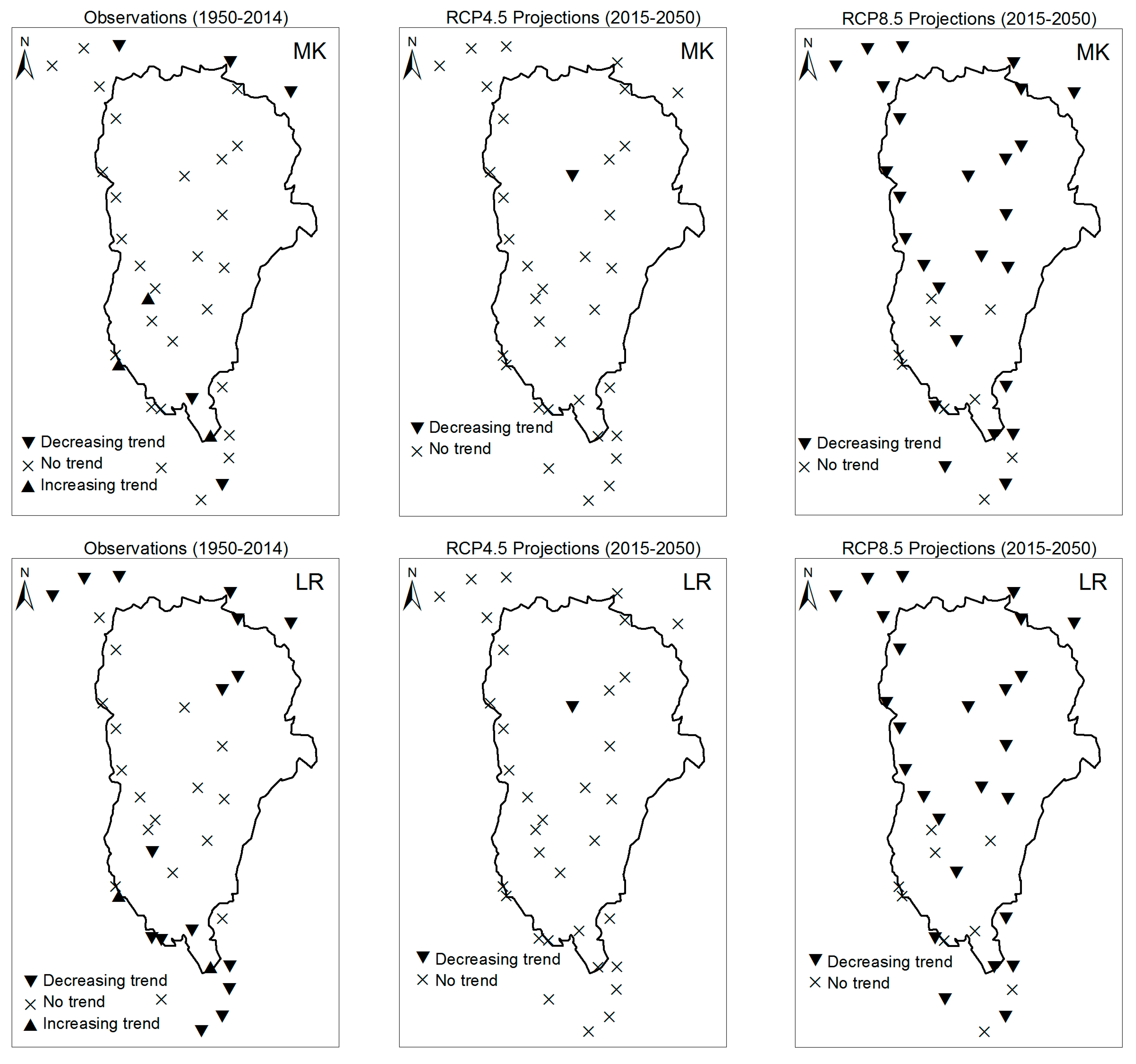
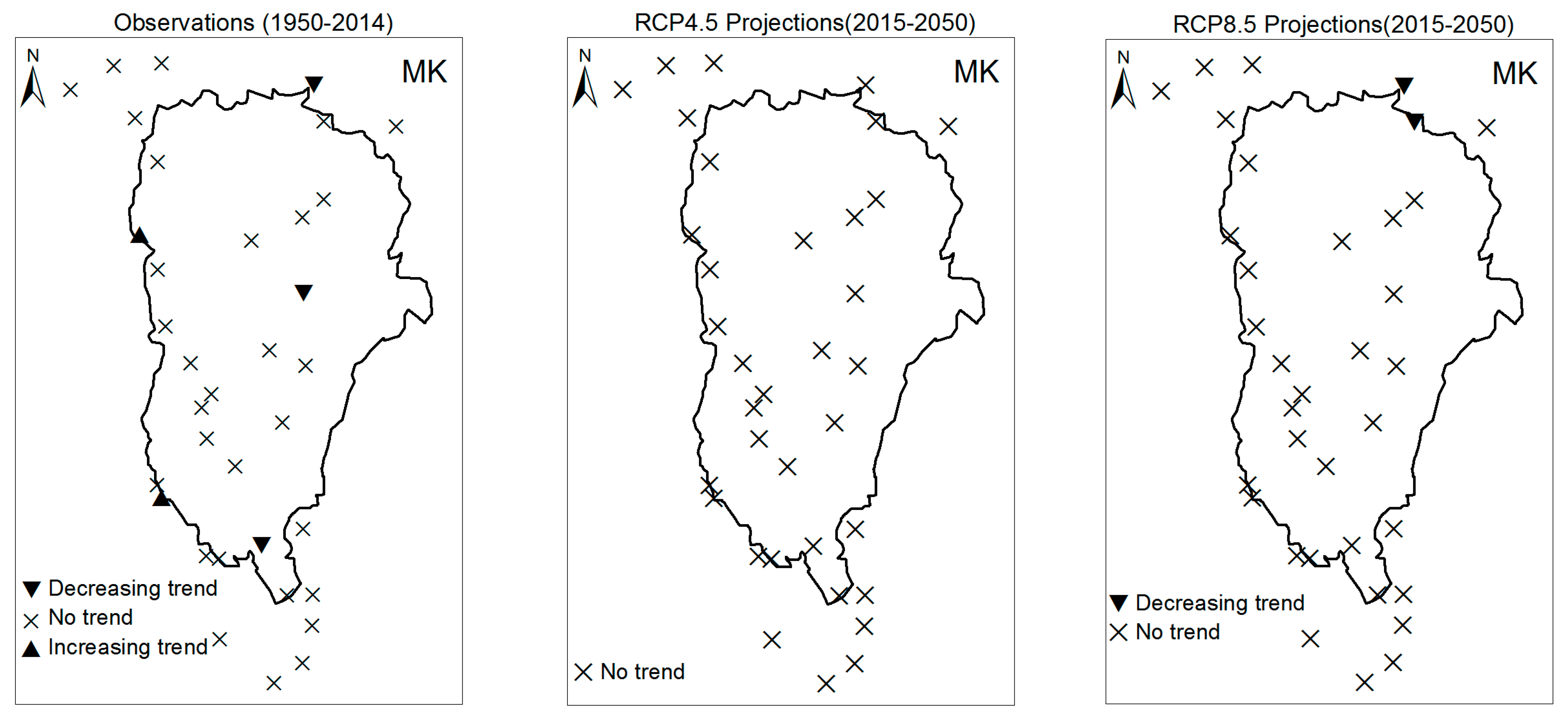
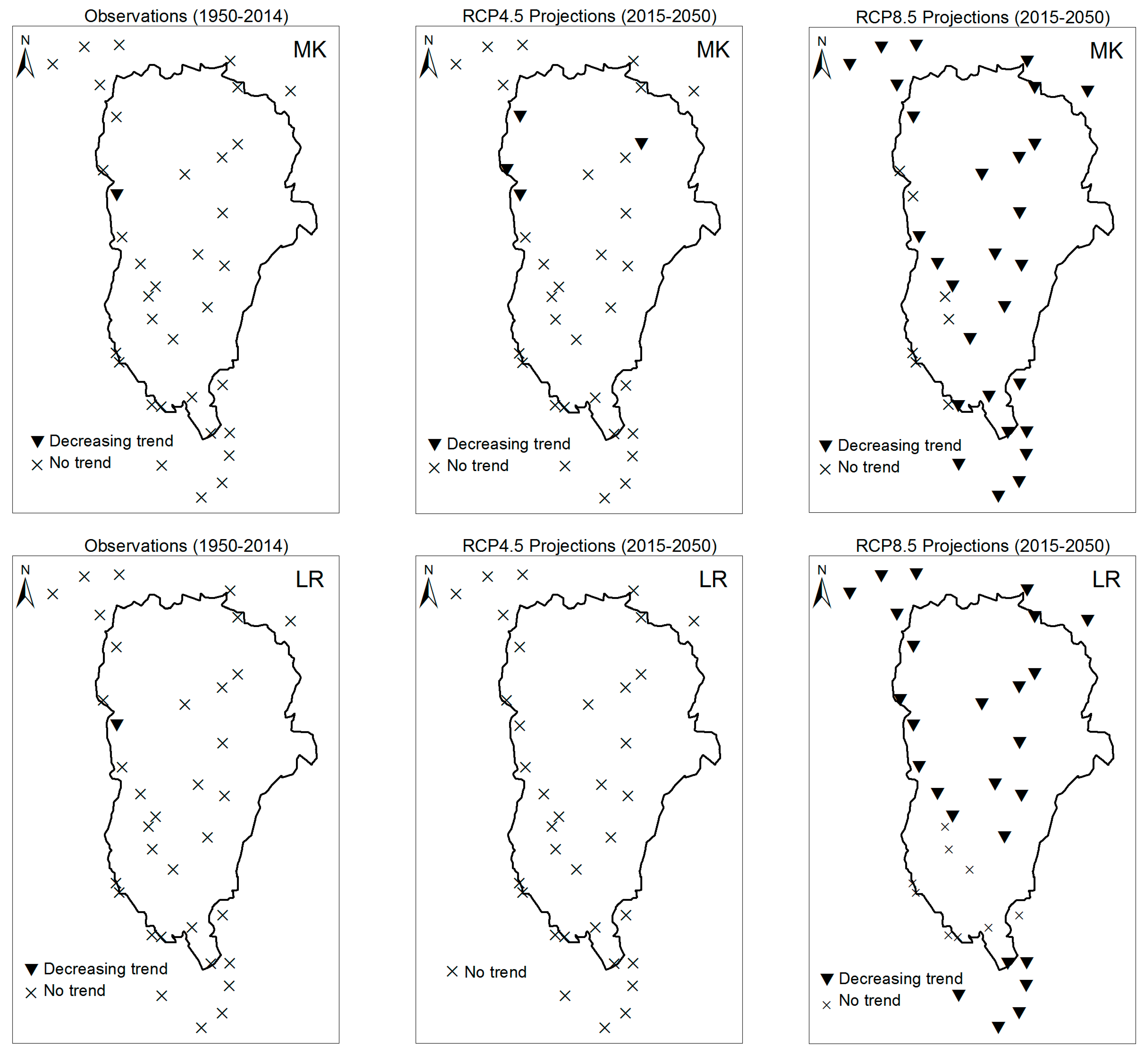
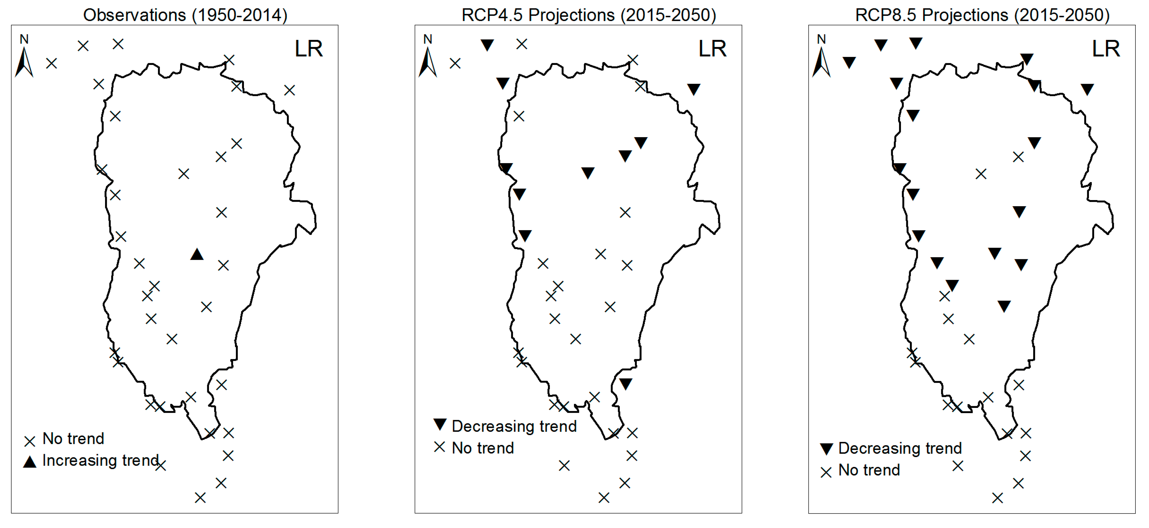
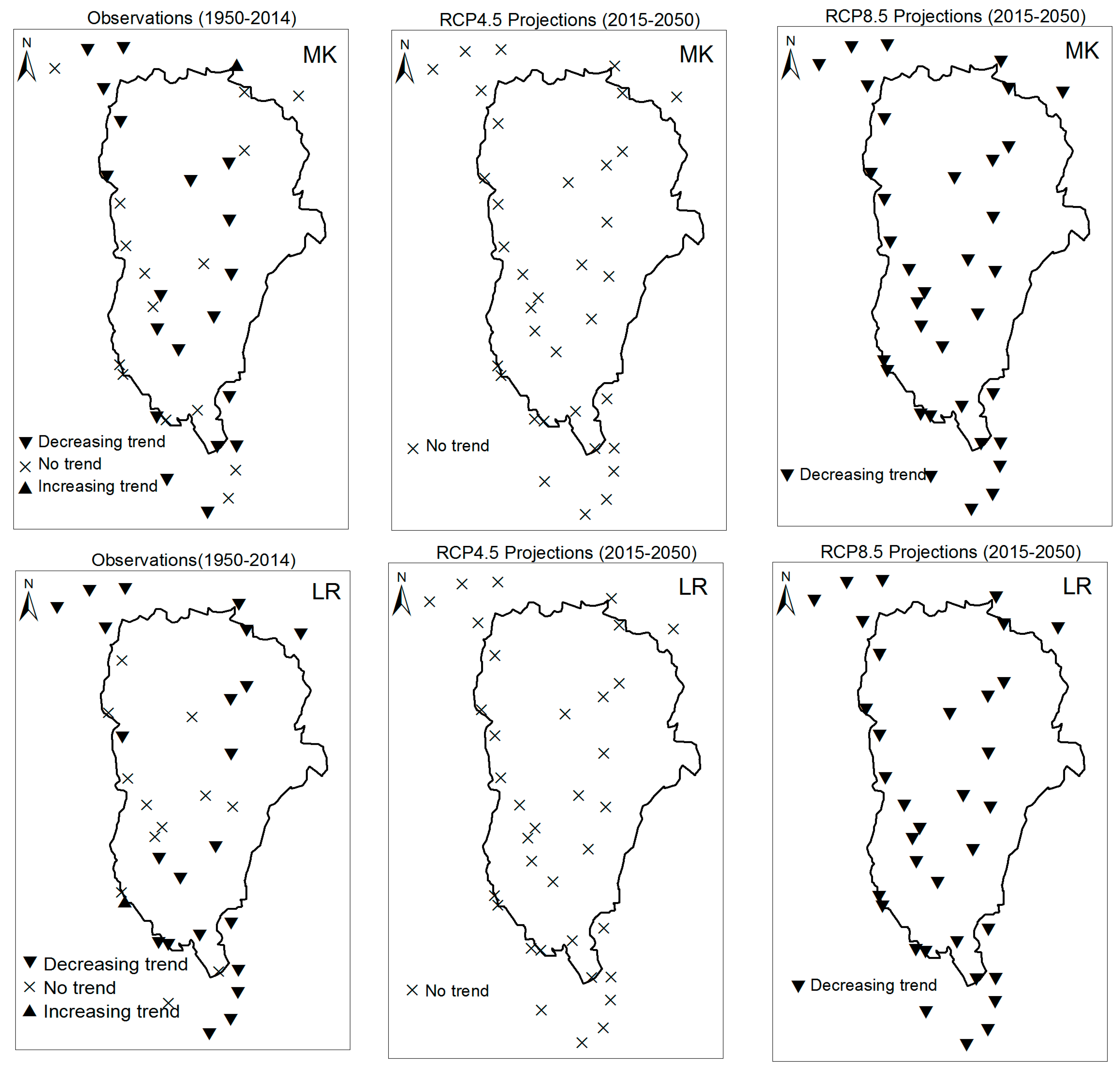
3.1. Annual Past and Future Climate Indices Trends

Figure 2, Figure 3, Figure 4, Figure 5, Figure 6, Figure 7, Figure 8 and Figure 9 show the spatial distribution of rainfall indices trends while que

Table A1. Results of Mann-Kendall and Sen Tests for indices R1, R10, R20, CDD, CWD and PRCPTOT, period 1950–2014.

Stations	R1mm		R10mm		R20mm		CDD		CWD		PRCPTOT
	Z	β	Z	β	Z	β	Z	β	Z	β	Z	β
Abomey	−1.88	−0.26	−0.83	−0.04	−0.46	0.00	2.05	2.49	−1.13	0.00	−1.97	−1.37
Adjohoun	−1.98	0.00	−1.96	0.00	0.54	0.00	1.33	0.22	0.77	0.00	−1.96	−1.16
Agouna	−1.97	−0.17	1.87	0.55	3.35	0.36	0.13	0.04	−1.20	−0.05	1.67	9.22
Aklampa	−0.77	−0.60	−2.16	−0.25	0.28	0.00	0.11	1.40	−0.29	0.00	−2.12	−7.13
Bantè	0.74	0.06	0.86	0.05	1.47	0.06	1.95	0.61	1.11	0.00	0.30	0.53
Bassila	−4.44	−1.00	−1.32	−0.16	0.38	0.05	1.79	1.00	−1.85	−0.06	−1.53	−6.14
Bembèrèkè	−1.65	−0.24	1.98	−0.14	−2.73	−0.10	1.73	0.41	−2.33	−0.02	1.96	−4.45
Beterou	−2.36	0.00	−1.97	−0.08	−0.08	0.00	2.00	1.53	−1.97	0.00	−2.10	−0.36
Birni	−3.34	−0.55	−0.49	−0.04	0.08	0.00	1.23	1.00	−1.23	−0.04	−0.98	−3.32
Bohicon	−2.27	−0.18	−2.24	0.00	2.42	0.00	1.87	0.35	−2.69	−0.02	−1.96	−0.56
Bonou	−1.08	−0.71	1.78	0.31	1.90	0.28	2.18	0.33	−1.38	0.00	1.27	7.13
Boukombé	−4.61	−0.86	−1.98	−0.09	−0.21	0.00	1.88	0.79	−2.43	−0.04	−2.10	−3.11
Cotonou	−2.13	0.00	−2.10	0.00	−0.20	0.00	0.95	0.16	−2.80	−0.02	−1.99	−0.05
Dassa	−2.00	−0.27	−1.97	−0.09	0.95	0.05	0.87	0.25	−2.21	0.00	−2.30	−1.97
Djougou	−1.98	0.00	−2.31	0.00	0.52	0.00	1.29	0.53	−1.98	0.00	−1.96	−0.95
Gouka	1.34	0.42	1.08	0.17	2.07	0.30	−1.39	−0.97	1.08	0.00	−1.41	−9.81
Ina	−1.75	−0.46	−1.78	−0.22	−1.78	−0.11	2.69	1.13	−1.80	−0.03	−1.95	−6.95
Ketou	−2.30	0.00	−2.69	−0.10	0.40	0.00	1.78	0.88	−2.15	0.00	−1.98	−1.81
Kokoro	−1.98	−0.04	−1.97	−0.04	−2.01	0.00	1.67	0.81	−1.97	0.00	−2.17	−3.35
Kouandé	−2.10	−0.09	−1.05	−0.13	−1.87	−0.11	1.97	0.58	−1.96	0.00	−1.98	−2.89
Natitingou	−3.21	−0.10	−1.99	−0.07	−0.32	0.00	−0.56	−0.10	−2.49	−0.03	−2.10	−2.16
Nikki	−2.30	−0.11	−1.77	−0.18	−2.30	−0.13	1.44	0.53	−1.35	0.00	−1.89	−4.81
Okpara	−4.10	−0.16	−1.46	−0.10	−0.50	0.00	0.59	0.18	−0.43	0.00	−0.72	−1.47
Ouèssè	−0.89	−0.08	0.51	0.03	0.75	0.03	1.32	0.57	0.61	0.00	−0.29	−0.87
Parakou	−1.99	−0.06	−2.49	−0.08	−0.02	0.00	1.64	0.33	−2.27	0.00	−2.30	−0.39
Pénéssoulou	−3.22	−1.00	−1.98	−0.29	−0.11	0.00	0.76	1.33	−2.70	0.00	−1.97	−3.72
Pira	−2.04	0.00	−2.10	0.00	1.17	0.10	−0.25	−0.13	−3.22	0.00	0.33	1.50
Pobè	−2.17	−0.07	−1.96	−0.03	−1.31	−0.06	0.78	0.10	−2.10	0.00	−2.08	−1.59
Porto-Novo	−5.93	−0.82	−3.39	−0.23	−2.00	−0.08	1.96	0.32	−1.95	−0.06	−1.93	−6.67
Sakété	−2.39	−0.18	−1.90	−0.13	−0.66	−0.03	0.78	0.14	−2.11	0.00	−0.93	−1.86
Savalou	−1.98	−0.03	−2.28	−0.07	−1.11	−0.04	0.83	0.20	−1.96	0.00	−1.96	−1.85
Savè	−2.52	−0.20	−2.13	−0.02	0.59	0.00	1.16	0.21	−1.30	0.00	−2.14	−1.09
Tchaourou	−1.28	−0.46	−1.96	−0.10	−0.07	0.00	−1.96	0.00	−2.03	0.00	−3.20	−2.30
Tchètti	−4.30	−1.92	−2.30	−0.08	0.35	0.08	1.10	1.50	−3.45	−0.17	−0.63	−4.07
Zagnanando	1.31	0.17	−3.10	−0.08	−2.70	−0.05	1.70	0.50	−3.14	−0.30	−1.15	−2.83

,

Table A2. Results of Mann-Kendall and Sen tests SDII, RX1day, RX5day, R95pSUM and R99pSUM, period 1950–2014.

Stations	SDII		RX1day		RX5day		R95pSUM		R99pSUM
	Z	β	Z	β	Z	β	Z	β	Z	β
Abomey	1.35	0.02	0.99	0.15	−0.60	−0.16	0.03	0.05	0.98	0.00
Adjohoun	0.27	0.01	0.63	0.09	0.42	0.08	−0.11	−0.10	0.85	0.00
Agouna	4.21	0.29	2.71	1.74	2.36	2.25	2.09	3.04	2.69	4.34
Aklampa	−0.27	−0.10	−0.99	−2.12	−0.77	−2.96	−1.04	−6.33	−0.74	0.00
Bantè	−1.15	−0.02	−2.13	−0.39	−0.57	−0.14	−1.51	−1.89	−2.91	−1.48
Bassila	3.13	0.15	−0.23	−0.08	−2.01	−0.84	−0.29	−1.01	0.03	0.00
Bembèrèkè	−0.70	−0.01	−1.96	−0.30	−2.35	−0.59	−2.47	−2.08	−1.29	0.00
Beterou	1.97	0.02	0.94	0.28	0.05	0.03	0.19	0.33	0.90	0.00
Birni	2.32	0.09	−0.50	−0.14	−0.66	−0.33	−0.41	−0.44	0.23	0.00
Bohicon	2.77	0.03	0.96	0.14	1.04	0.20	1.43	1.38	0.79	0.00
Bonou	4.76	0.26	−0.12	−0.03	−0.19	−0.07	0.82	1.74	−0.21	0.00
Boukombé	1.87	0.11	1.01	0.28	−0.59	−0.28	−0.03	0.00	1.43	0.00
Cotonou	0.06	0.00	−0.95	−0.24	−1.28	−0.66	0.38	0.45	−0.28	0.00
Dassa	1.35	0.04	−0.32	−0.08	−0.65	−0.19	0.08	0.17	−0.34	0.00
Djougou	0.33	0.01	0.72	0.14	0.92	0.22	0.61	0.81	0.52	0.00
Gouka	0.82	0.06	0.67	0.57	1.61	1.90	1.22	6.84	0.64	0.00
Ina	−0.33	−0.01	−1.05	−0.27	−2.00	−0.54	−1.05	−1.85	−0.51	0.00
Ketou	−0.66	−0.01	−1.04	−0.17	−0.45	−0.11	−0.55	−0.61	−1.27	0.00
Kokoro	−0.03	0.00	0.95	0.51	1.67	0.94	1.02	3.34	0.45	0.00
Kouandé	−0.98	−0.02	0.03	0.00	0.21	0.07	0.55	0.68	0.43	0.00
Natitingou	−0.71	−0.01	−1.10	−0.12	−1.43	−0.15	−1.58	−1.55	−1.98	0.00
Nikki	−1.03	−0.04	−0.67	−0.16	−0.30	−0.13	−1.54	−2.26	−0.64	0.00
Okpara	0.72	0.02	0.90	0.23	−0.68	−0.14	0.08	0.08	0.83	0.00
Ouèssè	1.20	0.03	−0.04	−0.01	−0.06	−0.04	−0.23	−0.23	−0.39	0.00
Parakou	−0.81	−0.01	1.92	0.29	−0.01	0.00	1.00	0.85	1.62	0.00
Pénéssoulou	2.54	0.35	2.88	3.04	1.52	2.71	2.24	4.83	3.01	10.28
Pira	0.70	0.03	0.40	0.14	0.95	0.69	−0.09	−0.16	0.97	0.00
Pobè	−0.12	0.00	−0.75	−0.14	−1.25	−0.30	−0.47	−0.47	−0.84	0.00
Porto-Novo	3.76	0.10	−1.41	−0.34	−1.67	−0.70	−0.64	−1.29	−1.37	0.00
Sakété	0.44	0.01	−0.40	−0.08	−1.11	−0.30	0.12	0.25	−0.65	0.00
Savalou	−1.14	−0.02	0.68	0.24	0.93	0.23	−0.36	−0.76	0.64	0.00
Savè	1.61	0.02	−0.10	−0.02	−1.36	−0.27	−0.85	−0.71	0.03	0.00
Tchaourou	1.71	0.04	−0.08	−0.03	−1.98	−0.48	−2.02	−1.64	−1.98	0.00
Tchètti	3.08	0.39	0.07	0.06	0.35	0.29	−0.49	−1.78	0.13	0.00
Zagnanando	−2.19	−0.08	−2.13	−0.22	−1.97	−0.30	−2.10	−1.06	−2.03	0.00

and

Table A3. Results of Mann-Kendall and Sen tests for the scenario RCP8.5, period 2015–2050.

Stations	R1		R10		R20		CWD		PRCPTOT
	Z	β	Z	β	Z	β	Z	β	Z	β
Abomey	−1.97	−2.00	−4.05	−0.06	−2.62	−2.95	−0.30	−0.40	2.30	−9.06
Adjohoun	−2.36	−12.96	−3.09	−0.45	−2.84	−3.17	−2.33	−3.37	1.98	−9.11
Agouna	−2.30	−2.92	−3.00	−1.25	−1.95	−1.70	−1.98	−0.90	1.98	−8.25
Aklampa	−1.96	−10.78	−1.96	−5.69	−2.15	−2.48	1.10	0.23	4.65	−15.38
Bantè	−3.00	−10.76	−5.25	−6.41	−2.15	−2.48	0.30	0.00	2.87	−14.83
Bassila	−1.96	−1.82	−5.21	−8.46	−1.96	−2.29	0.80	0.08	1.96	−20.92
Bembèrèkè	−1.17	−8.89	−2.00	−3.29	−3.01	−3.34	−1.25	−0.50	1.97	−5.58
Bétérou	−4.32	−9.91	−4.18	−8.25	−1.97	−2.30	−1.80	0.17	2.19	−20.50
Birni	−2.50	−9.93	−2.22	−5.47	−2.31	−2.64	0.08	0.00	2.27	−14.94
Bohicon	−2.30	−11.00	−2.09	−1.02	−1.80	−3.10	−1.96	−1.03	2.20	−13.02
Bonou	−1.99	−7.00	−6.23	−0.74	−3.00	−3.33	−2.07	−2.80	2.70	−9.74
Boukombé	−2.80	−5.98	−2.17	−4.66	−2.62	−2.95	−1.90	−0.34	2.10	−13.32
Cotonou	−4.20	−3.87	−4.09	−2.49	−1.05	−2.50	−3.02	−5.12	3.45	−2.99
Dassa-Zoumè	−1.98	−9.79	−2.07	−3.89	−3.08	−3.41	−1.97	−0.90	1.99	−8.79
Djougou	−2.00	−15.94	−3.12	−9.38	−1.98	−2.31	−1.23	−0.10	2.52	−18.77
Gouka	−3.22	−7.86	−2.10	−5.72	−1.70	−1.02	−0.90	0.00	2.57	−14.43
Ina	−1.98	−2.88	−4.00	−3.39	−1.96	−2.29	1.23	0.00	2.13	−5.78
Kétou	−2.01	−10.00	−2.06	−0.81	−2.80	−3.13	1.20	0.10	3.10	−7.39
Kokoro	−3.20	−13.89	−6.14	−3.22	−2.20	−2.53	−0.50	0.30	3.01	−9.44
Kouandé	−5.60	−15.97	−2.25	−6.46	−2.45	−2.78	−2.17	−3.20	1.96	−12.92
Natitingou	−3.10	−2.92	−5.21	−5.35	−2.54	−2.87	−1.40	−0.17	2.27	−14.69
Nikki	−2.10	−15.85	−3.14	−4.16	−3.12	−3.45	0.30	−3.00	3.43	−11.31
Okpara	−4.05	−2.83	−2.15	−6.23	−1.96	−2.29	1.80	0.13	4.25	−14.46
Ouèssè	−1.97	−8.00	−3.33	−5.83	−2.30	−2.63	−0.60	−0.01	1.96	−14.67
Parakou	−3.00	−3.93	−3.23	−6.26	−2.28	−2.61	−0.98	−0.20	2.83	−11.52
Pénéssoulou	−1.96	−11.79	−2.20	−9.58	−2.06	−2.39	−0.04	−0.09	1.96	−23.16
Pira	−4.03	−7.75	−3.27	−6.00	−2.51	−2.84	−0.21	−2.00	3.14	−12.00
Pobè	−2.37	−7.00	−1.89	−0.74	−2.07	−2.40	−3.60	−1.24	3.15	−7.74
Porto-Novo	−2.33	−12.95	−2.30	−0.52	−2.80	−3.13	−1.97	−0.02	4.36	−4.95
Sakété	−2.01	−10.91	−2.10	−2.31	−1.88	−0.50	−2.30	0.00	3.45	−6.61
Savalou	−4.77	−13.84	−3.10	−5.83	−1.40	−1.20	−1.97	−2.30	1.97	−13.67
Savè	−5.22	−13.87	−1.97	−5.95	−1.12	−0.80	−2.47	−4.60	2.22	−13.89
Tchaourou	−4.17	−7.00	−1.99	−6.34	−1.99	−2.32	−3.90	−0.20	1.98	−11.67
Tchetti	−2.44	−15.83	−1.98	−5.91	−1.94	−1.33	0.80	0.20	2.57	−15.83
Zagnanando	−2.35	−16.04	−1.97	−0.93	−1.06	−0.77	−1.98	−0.05	5.20	−11.93

give an overview of trends magnitudes. These indices were calculated at annual scale.

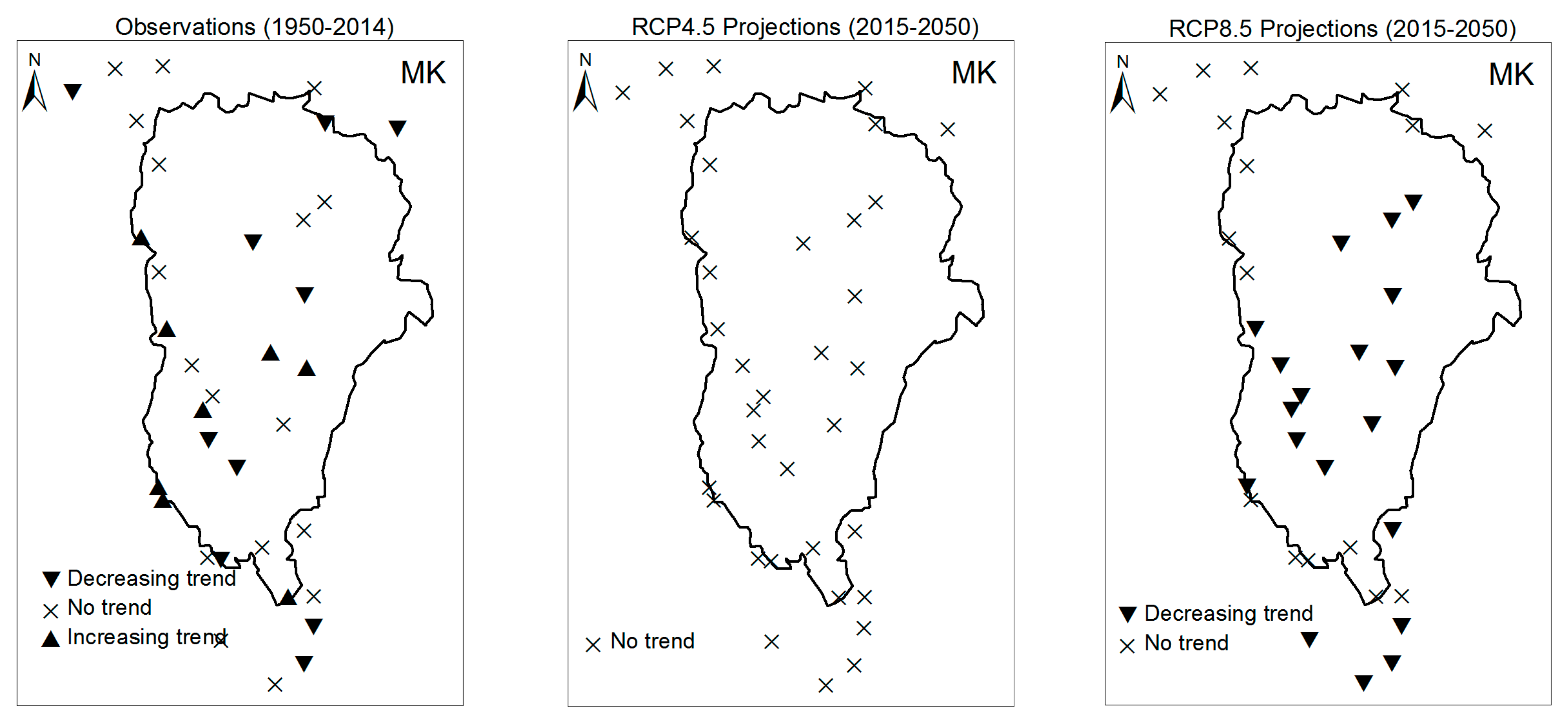
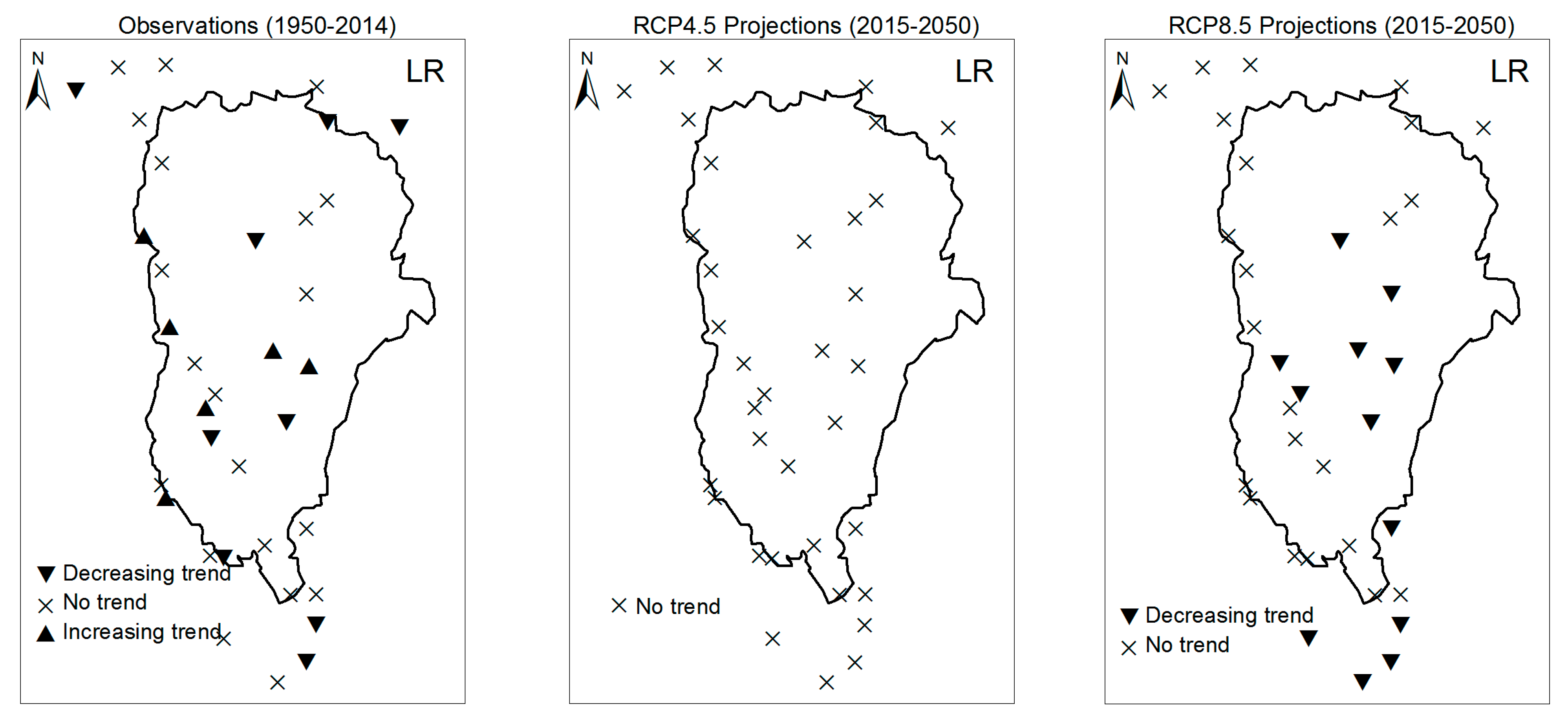
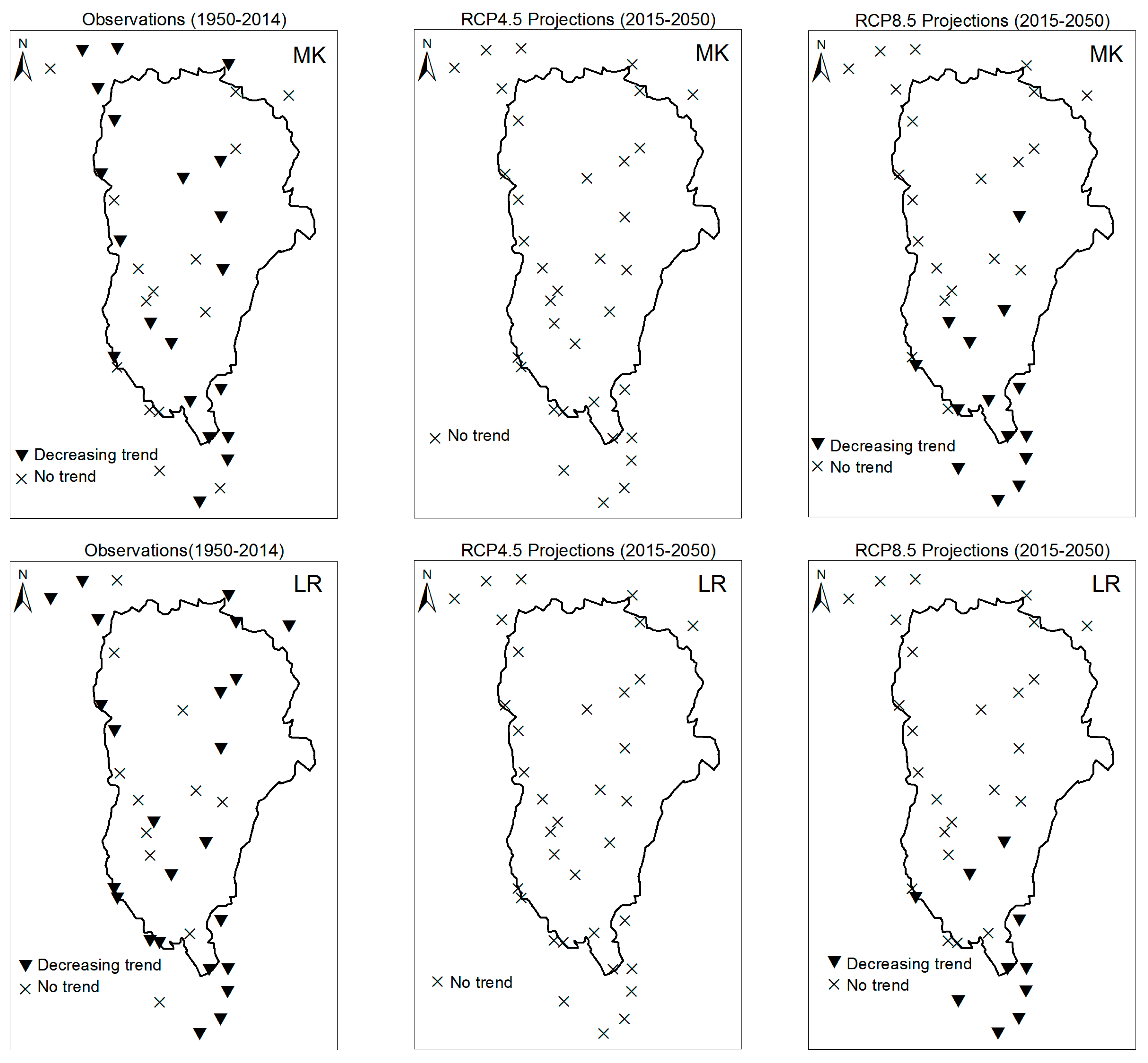
3.1.1. Annual Total Precipitation and Number of Wet Days

The annual indices were calculated at annual scale, this means that, one value of each index per year in each station. Thus, this study had 65 index values from 1950 to 2014 per station. The Figure 2 and Figure 3 show respectively the spatial distribution of observed and predicted annual total precipitation (PRCPTOT) and annual number of wet days (R1mm) trends in Ouémé basin. For the period 1950–2014 (observation period), most stations experienced a decreasing trend of PRCPTOT. Mann-Kendall (MK) test detected 52.3% stations at 5% significance level which faced this significant negative trend against about 63% stations detected by the linear regression (LR) test for the same significance level (Figure 2). The decline depends on station and it reaches 7 mm/year for some stations (Table A1). For the projected period (2015–2050), both statistical are coherent. Therefore, the annual total precipitation (PRCPTOT) will decrease in all stations for RCP8.5 scenario and no significant trend will be noted in basin for RCP4.5. The findings for the scenario RCP4.5 characterize this scenario which states in a stabilized radiative forcing at 4.5 W/m² until year 2100 without ever exceeding that value. Following IPCC scenario RCP8.5, Ouémé watershed will face the continuous decreasing of annual total precipitation until 2050. The magnitude of the decreasing varies from −23 mm to −3 mm per year (Table A3).

As PRCPTOT index, a significant decreasing trend was noted in most stations for R1mm index (Figure 3). At 5% significance level, Mann-Kendall test indicates a significant decreasing trend for 71% stations and the linear regression detects 74% stations which also faced the significant negative trend from 1950 to 2014. However, the magnitude of the decline is negligible (the average is −0.3 day/year). No significant trend for RCP4.5 and 100% stations will experience the decrease of this index under the scenario RCP8.5. The decline average is estimated at 9.27 days/year during the period 2015–2050 following this extreme scenario (Table A3).

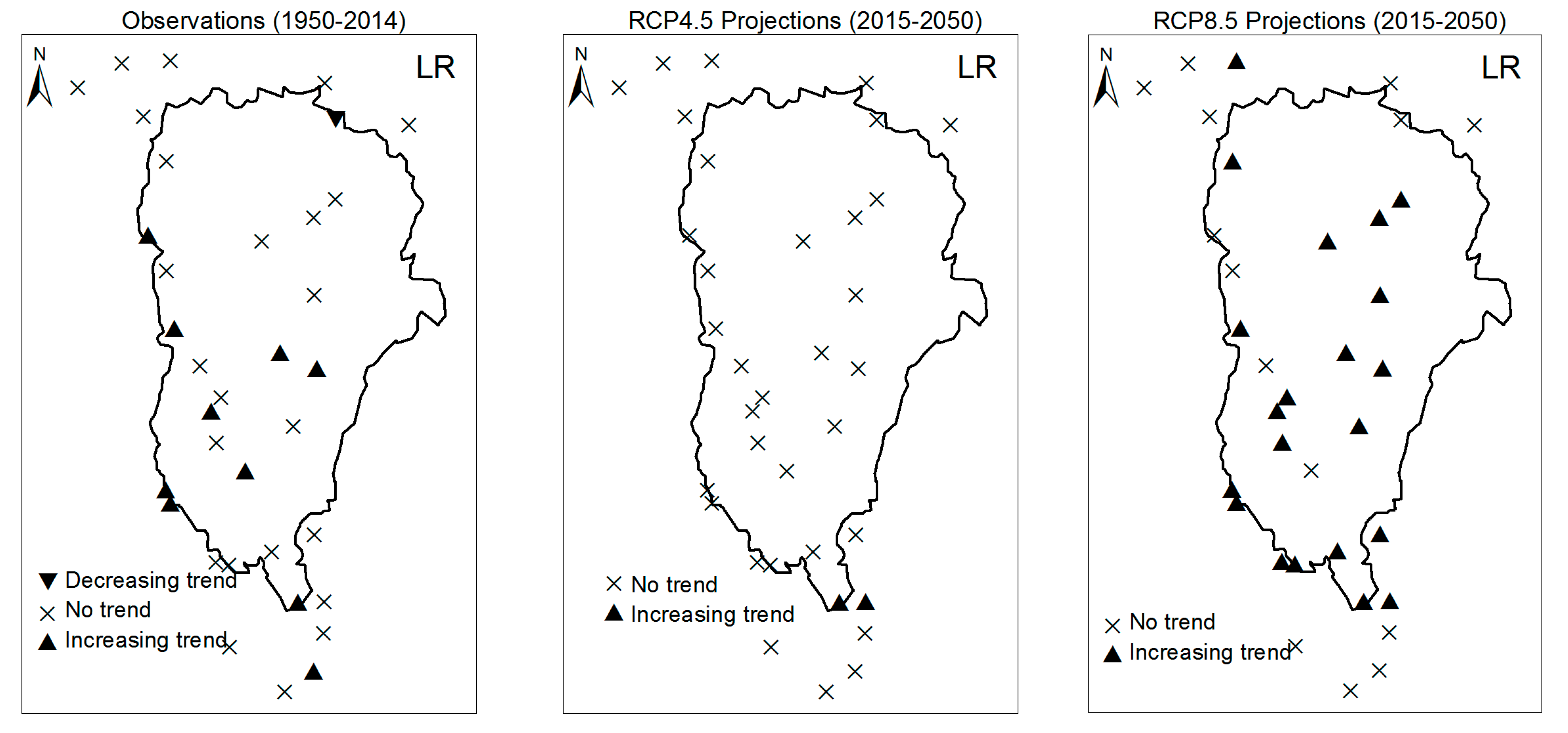
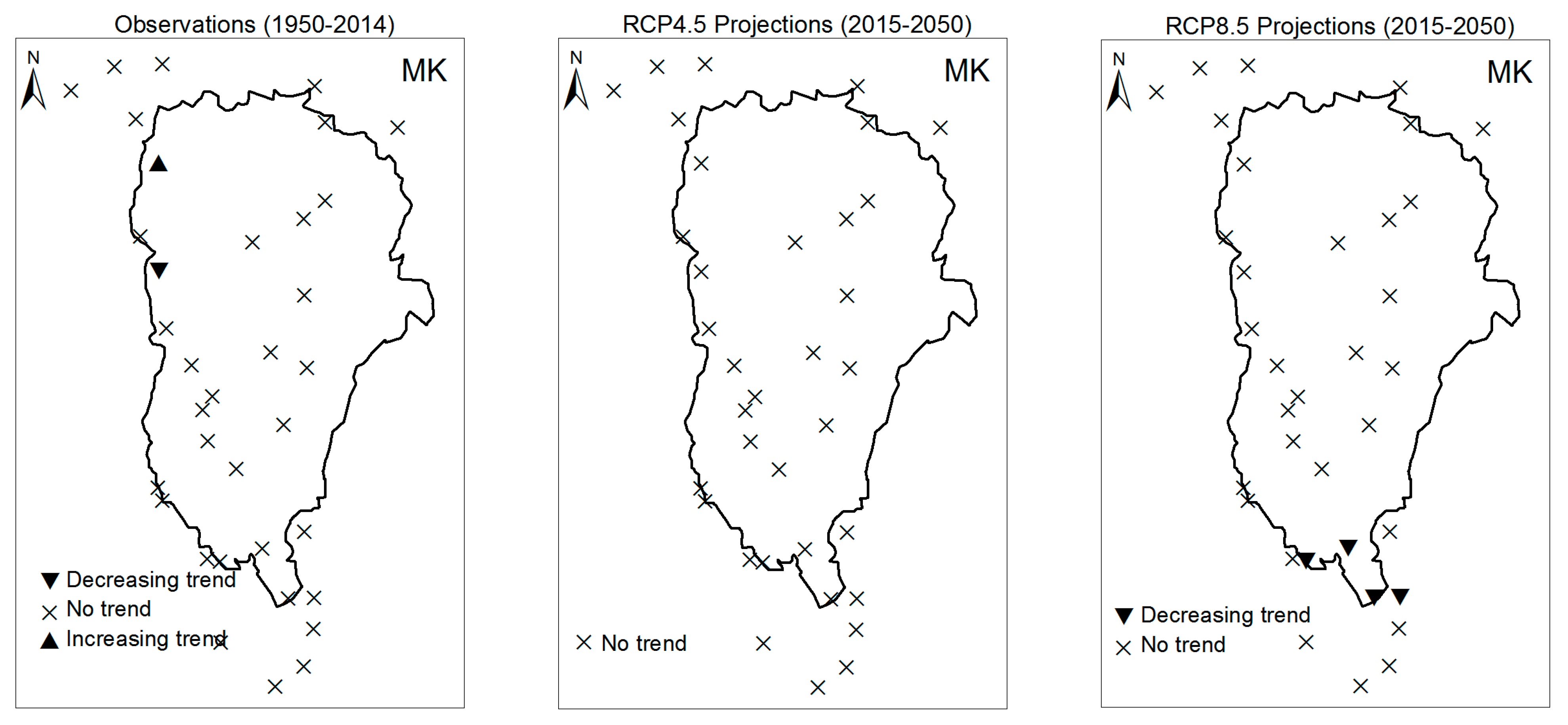
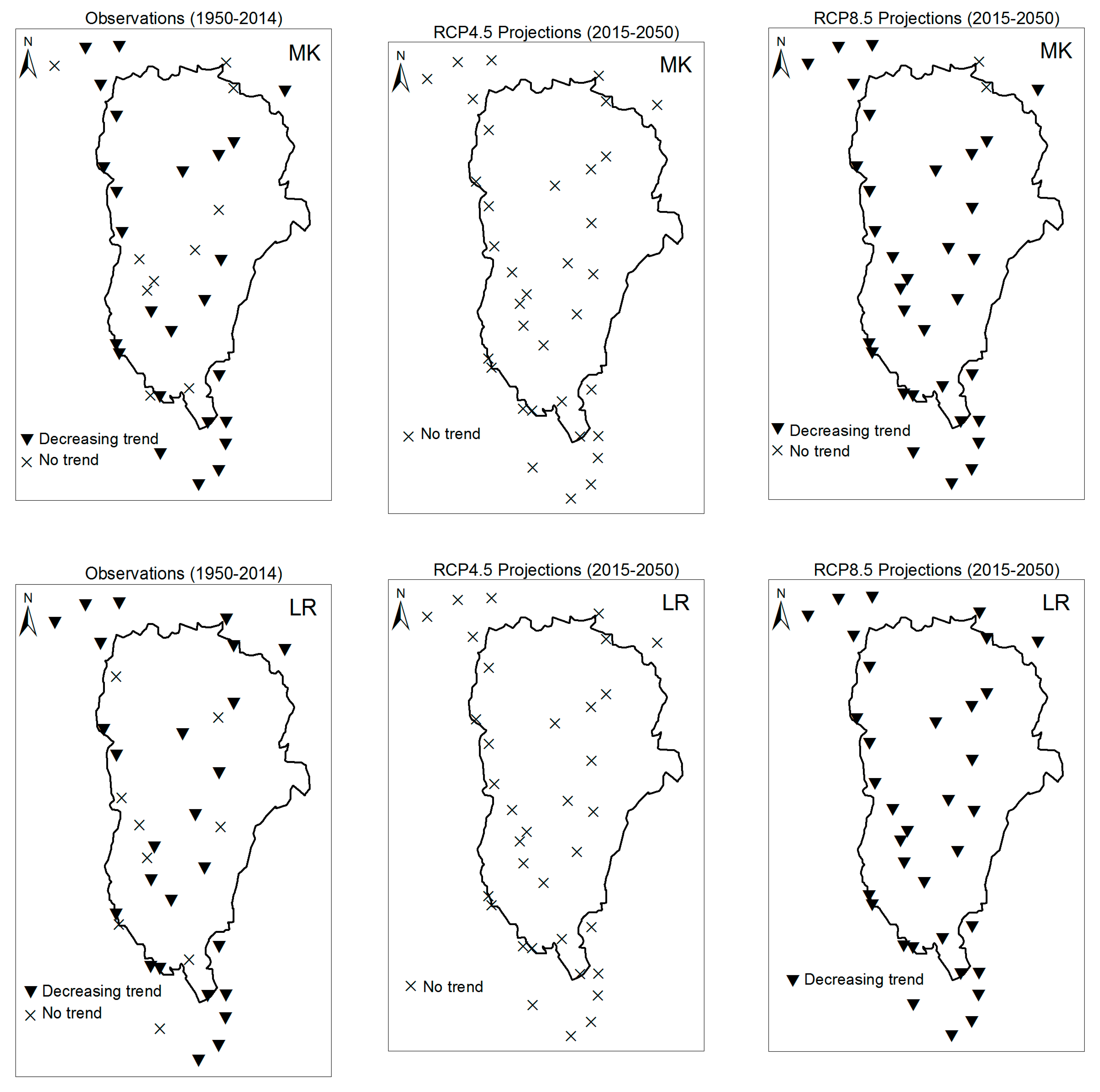
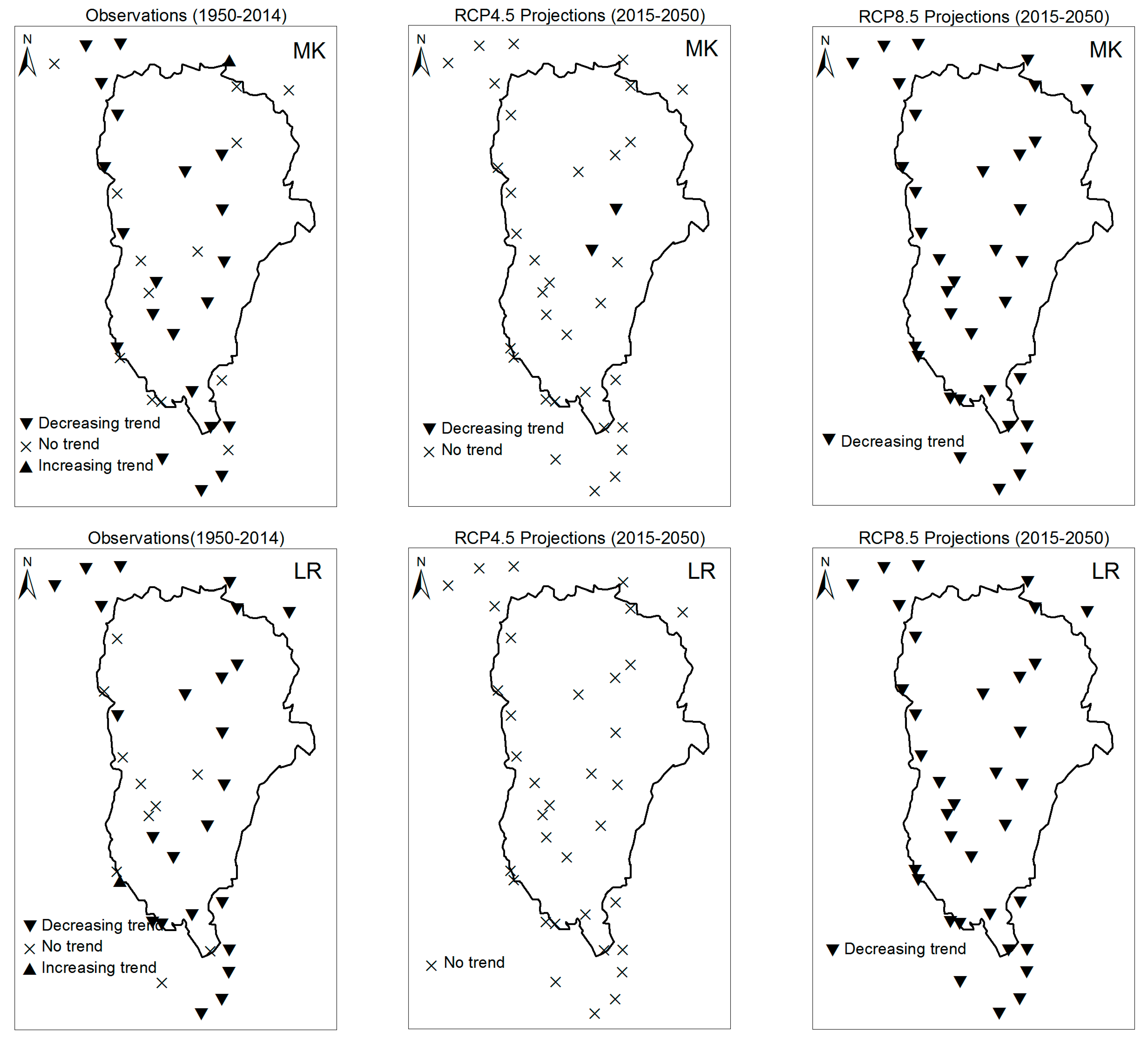
3.1.2. Consecutive Cumulative Wet Days and Heavy Precipitation

For the maximum consecutive wet day (CWD), the significant decreasing was detected for 57% and 68% stations by Mann-Kendall and linear regression tests respectively for the observation period (Figure 4). These stations are distributed across the whole basin but the decline magnitude is inconsiderable (Table A2). The future period 2015–2050, some stations would be characterized by a decrease trend of this index for the scenario RCP8.5 but no clear trend is detected for the scenario RCP4.5.

Figure 5 and Figure 6 displays the spatial distribution of trends for R10mm and R20mm indices, respectively. As the indices PRCPTOT, R1mm and CWD, the number of heavy precipitation days (R10mm) has significantly decreased in 60% and 68% stations such as detected by Mann-Kendall and linear regression methods respectively between 1950 and 2014. This reduction is not important (less than 0.5 day/year, Table A2). No significant trend is detected for the scenario RCP4.5 except two stations for the Mann-Kendall test. In the case of the scenario RCP8.5, the significant decreasing is detected in whole basin. The decline is estimated at −4.37 days/year in whole basin (Table A3).

For the number of very heavy precipitation days (R20mm), few stations experienced decreasing trend. For this index, Mann-Kendall test has identified 11% stations which faced a significant decreasing trend from 1950 to 2014 against 45% detected linear regression method (Figure 6). Except one, others stations didn’t present a significant trend for the scenario RCP4.5. Contrary to PRCPTOT, R1mm, CWD and R10mm, for R20mm index, there is no significant trend for some stations (26% stations) for RCP8.5 scenario.

The very wet day rainfall (R95pSUM) and the extremely wet day rainfall (R99pSUM) presented the significant decline for some stations from 1950 to 2014 (Figure 7 and Figure 8). Approximately, 45% stations were detected by linear regression against 11% stations by Mann-Kendall. In the whole, there is no trend detected by both statistical methods for projected data.

Regarding the simple daily intensity index (SDII), the increasing trends are detected for about 20% stations by Mann-Kendall test and 26% stations with the linear regression model. These stations are situated in western part of basin. There are also the decreasing trends for some stations majority detected with linear regression model. For RCP4.5 and RC8.5 scenarios few stations exhibited the trends. Only 8% stations located in southern part of basin for the scenario RCP4.5 and 10% stations all situated in north of basin for RCP8.5 were identified (Figure 9).

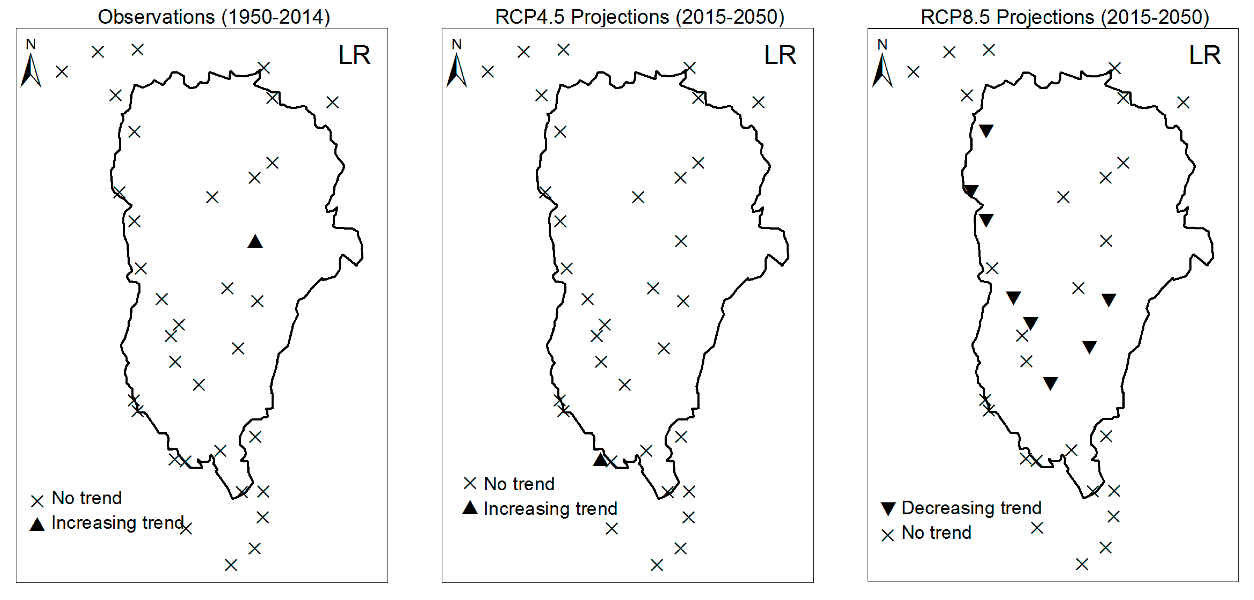
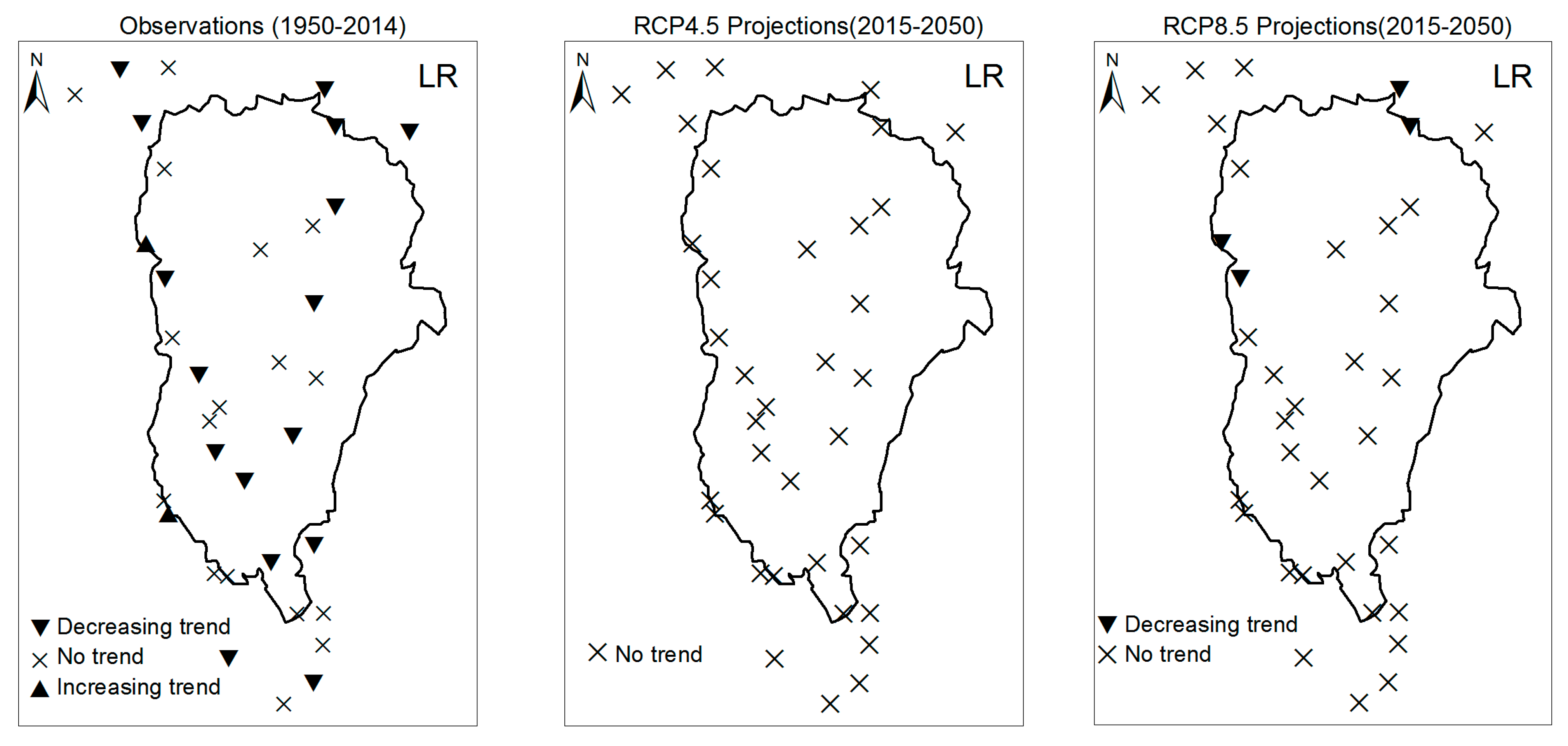
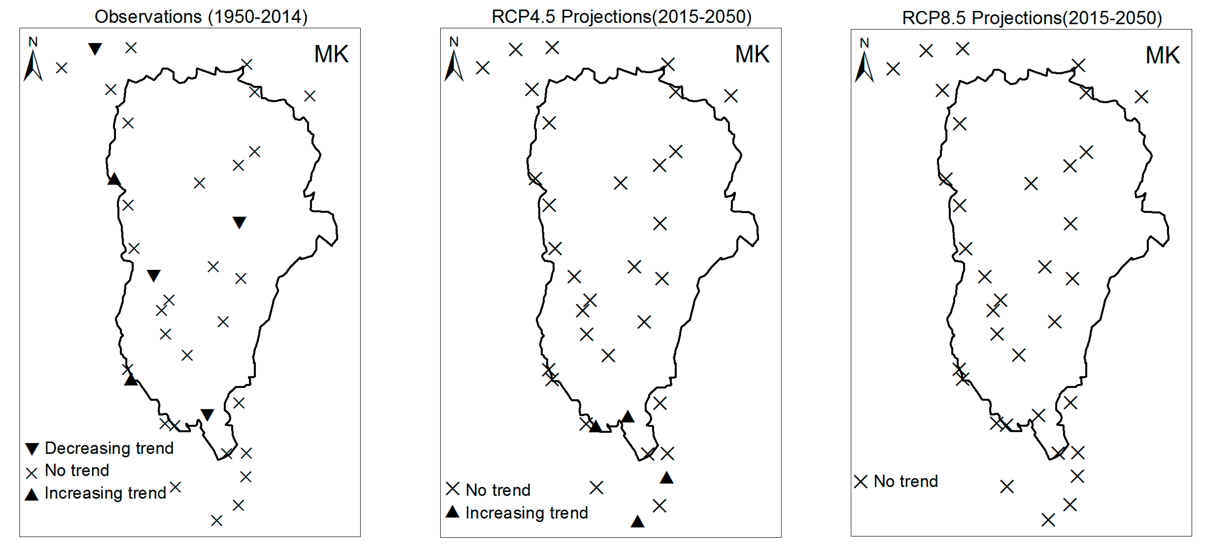
3.2. Rainy Season Past and Future Climate Index Trends

July to September is the heavy precipitation period in Ouémé watershed. Most of annual total precipitation is recorded in this period of year. For the period 1950–2014, about 56% of annual total rainfall was recorded from July to September. In general, more than 95% of annual rainfall is recorded between April and October. To apprehend the climate variability, we calculated the climate indices considering this sequence of year.

Contrary to the case of annual scale, there is no significant trend for the indices PRCPTOT, R10mm and R20mm calculated at rainy seasonal scale (July–August–September) in observation period for most stations (Figure 10, Figure 11 and Figure 12). This is also the case of the projected precipitation under RCP4.5 scenario. However, for the especially case of R20mm, few stations are affected by negative trend under this scenario compared to annual scale (Figure 12). The significant trends (here the negative trends) detected by both statistical methods used at annual scale for RCP8.5 predicted precipitation, are also detected for the seasonal scale in most stations (Figure 10, Figure 11 and Figure 12). These results mean that the annual total precipitation decreasing is related to heavy rainfall period, July–September.

For the maximum of number of consecutive wet days (CWD), some stations experienced a significant increasing for the period 1950–2014 at season scale. Mann-Kendall test detected 22% stations which experienced the significant positive trend against 17% stations identified by linear regression approach (Figure 13). These stations are situated in Midwest of basin. The significant negative trends are also detected for 28% stations by Mann-Kendal method and 26% stations with linear regression approach. There is no significant trend for RCP4.5 predicted data. However, for RCP8.5, the significant decreasing was identified for 51% stations using the Mann-Kendall test and 34% stations with linear regression.

The maximum of consecutive dry days (CDD) has significantly decreased in 34% stations as detected by Mann-Kendall method against 28% stations for linear regression during the period 1950–2014 (Figure 14). Therefore, most of stations didn’t experience a significant trend in rainy season in the observation period. However, in the case of RCP8.5 scenario, most stations will face the significant increase. The Mann-Kendall test and the linear regression detected respectively 83% and 63% stations which will experience the increasing of CDD index. There is no significant trend for RCP4.5 scenario.

Contrary to other indices at seasonal scale, there is no significant trend for maximum one-day precipitation (RX1day) and five-day precipitation (RX5day) indices for the period 1950–2014 (Figure 15 and Figure 16). Of the same, no station presents the significant trend for the RCP4.5 scenario in the whole basin. However, for RCP8.5 scenario, some stations of southern part of the basin, which is in a coastal area, exhibit the decrease trends for RX1day index. For RX5day, 37% stations showed a decreasing trend with the Mann-Kendall test whereas 23% stations were detected with the linear regression.

4. Discussion

We calculated the climate extremes indices in Ouémé watershed, the largest basin of Benin, and their changes from 1950 to 2014. Daily observational data from weather stations across the study area were subjected to quality control and processing, before calculating climate indices representative of different aspects of extreme climate events. Using REMO projections corrected data we also evaluated the future trends of theses indices. The lack of long-term climate data suitable for analysis of extremes is generally the biggest obstacle to quantifying whether extreme events have changed over the last decades in Africa [51]. Despite everything, we analysed the climate indices at various time scales (annual and seasonal) in the biggest and most gauged basin in Benin. The trends analysis was carried out using two statistical tests; the Mann-Kendall (MK) test and the Linear Regression (LR). It is worth noting that LR detected more significant trends than MK. That is mainly related to its high sensitivity to outliers due to the parametric character of the test. This concern is general with parametric tests like LR [53] of which the results are often influenced by the outlying observations. The normality hypothesis of data required by LR would not be respected. MK has low sensitivity to abrupt breaks due to inhomogeneous time series [49], so the trends estimated by this test illustrate more the real situation. The results give evidence for significant changes in the occurrence of climate extremes during the past six decades (1950–2014). In the whole, these changes are the decreasing trends in the basin for most indices; CDD experienced the increasing trends. However, the changes are spatially much contrasted and many stations didn’t present significant trends. These results are close to the findings of New et al. [3]. They showed that most precipitation indices do not exhibit consistent or statistically significant trends across West Africa. Due to the high proportion of stations without trends (no significant trends) the precipitation changes indices are spatially inconsistent. This same observation was highlighted for Northwest Africa to the Arabian Peninsula. It was emphasized by Donat et al. [14] who indicated that changes in precipitation are generally less consistent and characterized by a higher spatial and temporal variability; the trends are generally less significant. The spatially inconsistent trends of climate indices noticed are likely linked to the high heterogeneousness of the rainfall. Indeed, the Ouémé basin is characterized by two types of rainfall regimes. In southern part of basin there are two rainy seasons, the first one between mid-March to mid-July and the last one start in mid-August to October. As for the northern part of basin, it rains during one period, from April to October. The difficulty in detecting changes in extreme rainfall could be related to the high inter-annual natural variability of rainfall in basin. This difficulty has also been highlighted by Soro et al. [19] in Ivory-Coast and Aguilar et al. [17] in Guinea Conakry. The trends which are underlined here are also in accordance with the findings of Soro et al. [19] who showed the declining trends of climate index across Ivory-Coast. It has been shown that all precipitation indices have declined over the last decades in Djibouti, although only the very wet day frequency and the very wet day proportion present a significant decline [51]. The increasing of dry spell duration revealed was also indicated by New et al. [3] for West Africa. Likewise rainfall during the months of June to September appears to have witnessed declining trends over 1961–1993 in Nigeria [54]. In Benin, the work on climate indices made by Hountondji et al. [21] showed that only the annual total precipitation, the annual total of wet days and the annual maximum rainfall recorded during 30 days present a significant decreasing trend while the others rainfall indicators appear to remain stable for the period 1960–2000.

After the bias correction, the probability of detecting a climate change signal is reduced since the signal is reduced after the correction, but the variability remains [39,43]. The future indices calculated for the period 2015–2050 didn’t exhibit the significant trends for the scenario RCP4.5. These findings characterize the nature of this scenario described as stable scenario. In this uncertain future climate following RCP4.5 scenario, the people of basin who are mainly the farmers, will face difficulties to determine the adapted periods of year corresponding to different cultivations. In opposite, the decreasing trends for annual total precipitation (−12 mm/year), the number of heavy (−4.32 days/year) and very heavy precipitation days (−2.7 days/year), the maximum of consecutive wet days have showed the significant for most stations following the RCP8.5 scenario. These results are in line with Dosio and Panitz [55] using the regional climate model CCLM, have predicted a significant reduction of precipitation at the end of the century in West Africa. It is also in line with the recent special IPCC report which states that West Africa will likely experience longer and more intense droughts in the near future [56]. In RCP8.5 context, the agricultural sector, main economic activity in Ouémé watershed would be affected. Furthermore, a significant decrease in water availability (surface water and groundwater) due to a decrease in rainfall showed by [57] will exacerbate following the scenario RCP8.5. The reduction of inflow will affect economic activities in basin. The river discharges are the most important component of hydrological cycle for water planning and management in Ouémé basin. Indeed, due to financial and technological constraints hindering a satisfactory development, and exploration of groundwater and reservoir resources in Ouémé basin, river water is the most accessible water for many uses such as irrigation, livestock watering, washing. So all these activities will be affected.

5. Conclusions

We examined at annual and rainy season scale, eleven rainfall indices trends using the Mann-Kendall statistical test and the linear regression approach. These tests are applied to detect the trends at 95% confidence level. Increasing consecutive dry days was revealed indicating the reduction of rainy season length. The other indices showed less statistical significance at rainy season scale. Overall, at the annual scale, R1mm, R10mm, R20mm, CWD and PRCPTOT presented the significant declining for many stations. However the high proportion of stations with the no significant trends for many indices confirms that changes in precipitation are generally less consistent and characterised by a higher spatial and temporal variability. No significant future trend was detected for the RCP4.5 scenario contrary to the scenario RCP8.5 for which the frequency of heavy precipitation days, the maximum consecutive wet days and the annual total precipitation will face reduction. This study fills important gaps in the global picture of how the types of extremes precipitations are changing and the high proportion of stations with the inconsistent trends invites the planners to get ready for an uncertain future climate.

References

1. Ogountundé, P.G.; Friesen, J.; van de Giesen, N.; Savenije, H.H.G. Hydroclimatology of the Volta River Basin in West Africa: Trends and variability from 1901 to 2002. Phys. Chem. Earth 2006, 31, 1180–1188. [Google Scholar] [CrossRef]
2. Houghton, J.T.; Meira Filho, L.G.; Callander, B.A.; Harris, N.; Kattenberg, A.; Maskell, K. Climate Change. The IPCC Second Assessment Report; Cambridge University Press: New York, NY, USA, 1996; p. 572. [Google Scholar]
3. New, M.; Hewitson, B.; Stephenson, D.B.; Tsiga, A.; Kruger, A.; Manhique, A.; Gomez, B.; Coelho, C.A.S.; Masisi, D.N.; Kululanga, E.; et al. Evidence of trends in daily climate extremes over southern and west Africa. J. Geophys. Res. 2006, 111, D14102. [Google Scholar] [CrossRef]
4. Oguntundé, P.G.; Abiodunb, B.J.; Lischeid, G. Rainfall trends in Nigeria, 1901–2000. J. Hydrol. 2011, 411, 207–218. [Google Scholar] [CrossRef]
5. Powell, E.J.; Keim, B.D. Trends in daily temperature and precipitation extremes for the Southeastern United States: 1948–2012. J. Clim. 2015, 28, 1592–1612. [Google Scholar] [CrossRef]
6. Kunkel, K.E.; Andsager, K.; Easterling, D.R. Long-term trends in extreme precipitation events over the conterminous United States and Canada. J. Clim. 1999, 12, 2515–2527. [Google Scholar] [CrossRef]
7. Suppiah, R.; Hennessy, K.J. Trend in total rainfall, heavy rain events and number of dry days in Australia, 1910–1990. Int. J. Climatol. 1998, 10, 1141–1164. [Google Scholar] [CrossRef]
8. Zhai, P.M.; Zhang, X.B.; Wan, H.; Pan, X.H. Trends in total precipitation and frequency of daily precipitation extremes over China. J. Clim. 2005, 18, 1096–1108. [Google Scholar] [CrossRef]
9. Tomassini, L.; Jacob, D. Spatial analysis of trends in extreme precipitation events in high-resolution climate model results and observations for Germany. J. Geophys. Res. 2009, 114, D12113. [Google Scholar] [CrossRef]
10. Rajeevan, M.; Bhate, J.; Jaswal, A.K. Analysis of variability and trends of extreme rainfall events over India using 104 years of gridded daily rainfall data. Geophys. Res. Lett. 2008, 35. [Google Scholar] [CrossRef]
11. Cantet, P. Impacts du Changement Climatique sur les Pluies Extrêmes par l’utilisation d’un Générateur Stochastique de Pluies. Ph.D. Thesis, Université Montpellier II, Montpellier, France, 2009. [Google Scholar]
12. Yazid, M.; Humphries, U. Regional Observed Trends in Daily Rainfall Indices of Extremes over the Indochina Peninsula fro m 1960 to 2007. Climate 2015, 3, 168–192. [Google Scholar] [CrossRef]
13. Bielec, Z. Long terme variability of thunderstorms and thunderstorms precipitation occurrence in Cracow, Poland, in the period 1896–1995. Atmos. Res. 2001, 56, 161–170. [Google Scholar] [CrossRef]
14. Donat, M.G.; Peterson, T.C.; Brunet, M.; King, A.D.; Almazroui, M.; Kolli, R.K.; Boucherf, D.; Al-Mulla, A.Y.; Nour, A.Y.; Aly, A.A.; et al. Changes in extreme temperature and precipitation in the Arab region: Long-term trends and variability related to ENSO and NAO. Int. J. Climatol. 2013. [Google Scholar] [CrossRef]
15. Ozer, A.; Ozer, P. Désertification au Sahel: Crise climatique ou anthropique? Bull. Séances l’Acad. R. Sci. d’Outre-Mer 2005, 51, 395–423. [Google Scholar]
16. Easterling, D.R.; Evans, J.L.; Groisman, P.Y.; Karl, T.R.; Kunkel, K.E.; Ambenye, P. Observed variability and trends in extreme climate events: A brief review. Bull. Am. Meteorol. Soc. 2000, 81, 417–425. [Google Scholar] [CrossRef]
17. Aguilar, E.; Aziz Barry, A.; Brunet, M.; Ekang, L.; Fernandes, A.; Massoukina, M.; Mbah, J.; Mhanda, A.; do Nascimento, D.J.; Peterson, T.C.; et al. Changes in temperature and precipitation extremes in western central Africa, Guinea Conakry, and Zimbabwe, 1955–2006. J. Geophys. Res. 2009, 114, D02115. [Google Scholar] [CrossRef]
18. Ozer, P.; Hountondji, Y.C.; Laminou Manzo, O. Evolution des caractéristiques pluviométriques dans l’est du Niger de 1940 à 2007. GEO-ECO-Trop 2009, 33, 11–30. [Google Scholar]
19. Soro, G.E.; Noufé, D.; Goula Bi, T.A.; Shorohou, B. Trend Analysis for Extreme Rainfall at Sub-Daily and Daily Timescales in Côte d’Ivoire. Climate 2016, 4, 37. [Google Scholar] [CrossRef]
20. Mason, S.J.; Waylen, P.R.; Mimmack, G.M.; Rajaratnam, B.; Harrison, J.M. Changes in extreme rainfall events in South Africa. Clim. Chang. 1999, 41, 249–257. [Google Scholar] [CrossRef]
21. Hountondji, Y.-C.; De Longueville, F.; Ozer, P. Trends in extreme rainfall events in Benin (West Africa), 1960–2000. In Proceedings of the 1st International Conference on Energy, Environment and Climate Changes, Ho Chi Minh City, Vietnam, 26–27 August 2011. [Google Scholar]
22. Hounkpè, J.; Diekkrüger, B.; Badou, D.F.; Afouda, A.A. Change in Heavy Rainfall Characteristics over the Ouémé River Basin, Benin Republic, West Africa. Climate 2016, 4, 15. [Google Scholar]
23. Nicholson, S.E. The West African Sahel: A Review of Recent Studies on the Rainfall Regime and Its Interannual Variability. ISRN Meteorol. 2013, 2013, 32. [Google Scholar] [CrossRef]
24. Tiedtke, M. A comprehensive mass flux scheme for cumulus parameterization in large-scale models. Mon. Weather Rev. 1989, 117, 1779–1800. [Google Scholar] [CrossRef]
25. Morcrette, J.J.; Smith, L.; Fourquart, Y. Pressure and temperature dependance of the absorption in longwave radiation parameterizations. Beitr. Phys. Atmos. 1986, 59, 455–469. [Google Scholar]
26. Giorgetta, M.; Wild, M. The Water Vapour Continuum and Its Representation in ECHAM4; Max-Planck Institut für Meteorologie: Hamburg, Germany, 1995. [Google Scholar]
27. Louis, J.-F. A parametric model of vertical eddy fluxes in the atmosphere. Bound.-Layer Meteor. 1979, 17, 187–202. [Google Scholar] [CrossRef]
28. Lohmann, U.; Roeckner, E. Design and performance of a new cloud microphysics scheme developed for the ECHAM4 general circulation model. Clim. Dyn. 1996, 12, 557–572. [Google Scholar] [CrossRef]
29. Hagemann, S. An Improved Land Surface Parameter Dataset for Global and Regional Climate Models; Max-Planck-Institute for Meteorology: Hamburg, Germany, 2002. [Google Scholar]
30. Rechid, D.; Raddatz, T.; Jacob, D. Parameterization of snow-free land surface albedo as a function of vegetation phenology based on MODIS data and applied in climate modelling. Theor. Appl. Climatol. 2009, 95, 245–255. [Google Scholar] [CrossRef]
31. The REMO Model. Available online: http://www.remo-rcm.de/059966/index.php.en#tab-10 (accessed on 18 September 2017).
32. Giorgi, F.; Jones, C.; Asrar, G. Addressing climate information needs at the regional level: The CORDEX framework. World Meteorol. Org. Bull. 2009, 58, 175–183. [Google Scholar]
33. Haensler, A.; Saeed, F.; Jacob, D. Assessing the robustness of projected precipitation changes over central Africa on the basis of a multitude of global and regional climate projections. Clim. Chang. 2013, 121, 349–363. [Google Scholar] [CrossRef]
34. Kaboré, E.; Nikiema, M.; Ibrahim, B.; Helmschrot, J. Merging historical data records with MPI-ESM-LR, CanESM2, AFR MPI and AFR 44 scenarios to assess long-term climate trends for the Massili Basin in central Burkina Faso. Int. J. Curr. Eng. Technol. 2015, 5, 1846–1852. [Google Scholar]
35. Sarr, M.A.; Seidou, O.; Tramblay, Y.; El Adlouni, S. Comparison of downscaling methods for mean and extreme precipitation in Senegal. J. Hydrol. Reg. Stud. 2015, 4, 369–385. [Google Scholar] [CrossRef]
36. Mbaye, M.L.; Hagemann, S.; Haensler, A.; Gaye, A.T.; Afouda, A. Assessment of Climate Change Impact on Water Resources in the Upper Senegal Basin(West Africa). Am. J. Clim. Chang. 2015, 4, 77–93. [Google Scholar] [CrossRef]
37. Giertz, S.; Höllermann, B.; Diekkrüger, B. An interdisciplinary scenario analysis to assess the water availability and water consumption in the Upper Ouémé catchment in Benin. Adv. Geosci. 2006, 9, 3–13. [Google Scholar] [CrossRef]
38. Nikulin, G.; Jones, C.; Giorgi, F.; Asrar, G.; Cerezo-Mota, M.; Christensen, O.B.; Déqué, M.; Fernandez, J.; Hänsler, A.; Meijgaard, E.V.; et al. Precipitation climatology in an ensemble of CORDEX-Africa regional climate simulations. J. Clim. 2012, 25, 6057–6078. [Google Scholar] [CrossRef]
39. N’Tcha M’Po, Y.; Lawin, A.E.; Oyerinde, G.T.; Yao, K.B.; Afouda, A.A. Comparison of Daily Precipitation Bias Correction Methods Based on Four Regional Climate Model Outputs in Ouémé Basin, Benin. Hydrology 2017, 4, 58–71. [Google Scholar] [CrossRef]
40. Paeth, H.; Born, K.; Podzun, R.; Jacob, D. Regional dynamic downscaling over Westafrica: Model evaluation and comparison of wet and dry years. Meteorol. Z. 2005, 143, 349–367. [Google Scholar] [CrossRef]
41. CORDEX Database. Available online: https://www.cordex.org (accessed on 18 September 2017).
42. Hagemann, S.; Chen, C.; Haerter, J.O.; Heinke, J.; Gerten, D.; Piani, C. Impact of a statistical bias correction on the projected hydrological changes obtained from three GCMs and two hydrology models. J. Hydrometeorol. 2011, 12, 556–578. [Google Scholar] [CrossRef]
43. Gutjahr, O.; Heinemann, G. Comparing precipitation bias correction methods for high-resolution regional climate simulations using COSMO-CLM. Effects on extreme values and climate change signal. Theor. Appl. Climatol. 2013, 114, 511–529. [Google Scholar] [CrossRef]
44. Amengual, A.; Homar, V.; Romero, R.; Alonso, S.; Ramis, C. A Statistical Adjustment of Regional Climate Model Outputs to Local Scales: Application to Platja de Palma, Spain. J. Clim. 2012, 25, 939–957. [Google Scholar] [CrossRef]
45. Obada, E.; Alamou, A.E.; Zandagba, E.J.; Biao, I.E.; Chabi, A.; Afouda, A.A. Comparative study of seven bias correction methods applied to three Regional Climate Models in Mekrou catchment (Benin, West Africa). Int. J. Curr. Eng. Technol. 2016, 6, 1831–1840. [Google Scholar]
46. Dai, A. Precipitation Characteristics in Eighteen Coupled Climate Models. J. Clim. 2006, 19, 4605–4630. [Google Scholar] [CrossRef]
47. Yazid, M.; Humphries, U.; Sudarmadji, T. Spatiotemporal of extreme rainfall events in the Indochina peninsula. In Proceedings of the International Conference on Applied Statistics, Khon Kaen, Thailand, 21–24 May 2014; pp. 238–245. [Google Scholar]
48. Zhang, X.; Hogg, W.D.; Mekis, E. Spatial and temporal characteristics of heavy precipitation events over Canada. Am. Meteorol. Soc. 2001, 14, 1923–1936. [Google Scholar] [CrossRef]
49. Tabari, H.; Somee, B.S.; Zadeh, M.R. Testing for long-term trends in climatic variables in Iran. Atmos. Res. 2011, 100, 132–140. [Google Scholar] [CrossRef]
50. Wang, Y.Q.; Zhou, L. Observed trends in extreme precipitation events in China during 1961–2001 and the associated changes in large-scale circulation. Geophys. Res. Lett. 2005, 32, L09707. [Google Scholar] [CrossRef]
51. Ozer, P.; Mahamoud, A. Recent Extreme Precipitation and Temperature Changes in Djibouti City (1966–2011). J. Climatol. 2013, 2013. [Google Scholar] [CrossRef]
52. Sen, P.K. Estimates of the Regression Coefficient Based on Kendall’s Tau. J. Am. Stat. Assoc. 1968, 63, 1379–1389. [Google Scholar] [CrossRef]
53. Muhlbauer, A.; Spichtinger, P.; Lohmann, U. Application and Comparison of Robust Linear Regression Methods for Trend Estimation. J. Appl. Meteorol. Climatol. 2007, 48, 1961–1970. [Google Scholar] [CrossRef]
54. Odekunle, O.T.; Adejuwon, A.S. Assessing changes in the rainfall regime in Nigeria between 1961 and 2004. GeoJournal 2007, 70, 145–159. [Google Scholar] [CrossRef]
55. Dosio, A.; Panitz, H.-J. Climate change projections for CORDEX Africa with COSMO-CLM regional climate model and differences with the driving global climate models. Clim. Dyn. 2016, 46, 1599–1625. [Google Scholar] [CrossRef] [Green Version]
56. Intergovernmental Panel on Climate Change. Summary for Policymakers. Climate Change 2014: Impacts, Adaptation, and Vulnerability; Contribution of Working Group II to the Fifth Assessment Report of the Intergovernmental Panel on Climate Change; Cambridge University Press: Cambridge, UK; New York, NY, USA, 2014. [Google Scholar]
57. Diekkrüger, B.; Diederich, M.; Giertz, S.; Höllermann, B.; Kocher, A.; Reichert, B.; Steup, G. Water availability and water demand under Global Change in Benin, West Africa. In Global Change and Water Resources in West Africa the German-African GLOWA Projects; Bundesministerium fur Bildung und Forschung: Ouagadougou, Burkina Faso, 2008. [Google Scholar]
Figure 1. Ouémé catchment.
Climate 05 00074 g001
Figure 2. Spatial distribution of annual total precipitation (PRCPTOT) observed (1950–2014) and projected (2015–2050) trends detected using Mann-Kendall (MK) and Linear Regression (LR) tests.
Climate 05 00074 g002
Figure 3. Spatial distribution of Annual number of wet days (R1mm) observed (1950–2014) and projected (2015–2050) trends.
Climate 05 00074 g003
Figure 4. Spatial distribution of Annual maximum cumulative wet days (CWD) observed (1950–2014) and projected (2015–2050) trends.
Climate 05 00074 g004
Figure 5. Spatial distribution of annual number of heavy precipitations (R10mm) days observed (1950–2014) and projected (2015–2050) trends.
Climate 05 00074 g005
Figure 6. Spatial distribution of annual number of very heavy precipitations days (R20mm) observed (1950–2014) and projected (2015–2050) trends.
Climate 05 00074 g006
Figure 7. Spatial distribution very wet day rainfall (R95pSUM) observed (1950–2014) and projected (2015–2050) trends.
Climate 05 00074 g007aClimate 05 00074 g007b
Figure 8. Spatial distribution of extreme rainfall (R99pToT) observed (1950–2014) and projected (2015–2050) trends.
Climate 05 00074 g008aClimate 05 00074 g008b
Figure 9. Spatial distribution of simple daily intensity index (SDII) observed (1950–2014) and projected (2015–2050) trends.
Climate 05 00074 g009
Figure 10. Spatial distribution of total precipitation (PRCPTOT) observed (1950–2014) and projected (2015–2050) trends for rainy season.
Climate 05 00074 g010
Figure 11. Spatial distribution of number of heavy precipitations days (R10mm) observed (1950–2014) and projected (2015–2050) trends for rainy season.
Climate 05 00074 g011
Figure 12. Spatial distribution of number of very heavy precipitations days (R20mm) observed (1950–2014) and projected (2015–2050) trends for rainy season.
Climate 05 00074 g012aClimate 05 00074 g012b
Figure 13. Spatial distribution of maximum consecutive wet day (CWD) observed (1950–2014) and projected (2015–2050) trends for rainy season.
Climate 05 00074 g013aClimate 05 00074 g013b
Figure 14. Spatial distribution of maximum consecutive dry day (CDD) observed (1950–2014) and projected (2015–2050) trends for rainy season.
Climate 05 00074 g014aClimate 05 00074 g014b
Figure 15. Spatial distribution of one-day maximum precipitation (RX1day) observed (1950–2014) and projected (2015–2050) trends for rainy season.
Climate 05 00074 g015aClimate 05 00074 g015b
Figure 16. Spatial distribution of wet season of five-day maximum precipitation (RX5day) observed (1950–2014) and projected (2015–2050) trends.
Climate 05 00074 g016aClimate 05 00074 g016b