The Relationship between Atmospheric Carbon Dioxide Concentration and Global Temperature for the Last 425 Million Years


1
Environmental Studies Institute, Boulder, CO 80301, USA
2
Division of Physical and Biological Sciences, University of California, Santa Cruz, CA 95064, USA
Climate 2017, 5(4), 76; https://doi.org/10.3390/cli5040076
Submission received: 8 August 2017
/
Revised: 15 September 2017
/
Accepted: 22 September 2017
/
Published: 29 September 2017
Abstract
:Assessing human impacts on climate and biodiversity requires an understanding of the relationship between the concentration of carbon dioxide (CO2) in the Earth’s atmosphere and global temperature (T). Here I explore this relationship empirically using comprehensive, recently-compiled databases of stable-isotope proxies from the Phanerozoic Eon (~540 to 0 years before the present) and through complementary modeling using the atmospheric absorption/transmittance code MODTRAN. Atmospheric CO2 concentration is correlated weakly but negatively with linearly-detrended T proxies over the last 425 million years. Of 68 correlation coefficients (half non-parametric) between CO2 and T proxies encompassing all known major Phanerozoic climate transitions, 77.9% are non-discernible (p > 0.05) and 60.0% of discernible correlations are negative. Marginal radiative forcing (ΔRFCO2), the change in forcing at the top of the troposphere associated with a unit increase in atmospheric CO2 concentration, was computed using MODTRAN. The correlation between ΔRFCO2 and linearly-detrended T across the Phanerozoic Eon is positive and discernible, but only 2.6% of variance in T is attributable to variance in ΔRFCO2. Of 68 correlation coefficients (half non-parametric) between ΔRFCO2 and T proxies encompassing all known major Phanerozoic climate transitions, 75.0% are non-discernible and 41.2% of discernible correlations are negative. Spectral analysis, auto- and cross-correlation show that proxies for T, atmospheric CO2 concentration and ΔRFCO2 oscillate across the Phanerozoic, and cycles of CO2 and ΔRFCO2 are antiphasic. A prominent 15 million-year CO2 cycle coincides closely with identified mass extinctions of the past, suggesting a pressing need for research on the relationship between CO2, biodiversity extinction, and related carbon policies. This study demonstrates that changes in atmospheric CO2 concentration did not cause temperature change in the ancient climate.
1. Introduction
Understanding the role of atmospheric carbon dioxide (CO2) in forcing global temperature is essential to the contemporary debate about anthropogenic global warming. Atmospheric CO2 and other trace gases emitted to the atmosphere by the combustion of fossil fuels and changes in land use patterns capture infrared energy radiated from the Earth’s surface, warming the atmosphere and surface by the “greenhouse” effect. Anthropogenic emissions of CO2 accelerated at the start of the Industrial Age in the mid-18th century and are now increasing the atmospheric concentration of CO2 by 1–2 parts per million by volume (ppmv) annually [1], a rate of increase that may be unprecedented in recent climate history. Over this same period the Earth has warmed by ~0.8 °C [2]. A central question for contemporary climate policy is how much of the observed global warming is attributable to the accumulation of atmospheric CO2 and other trace greenhouse gases emitted by human activities.
The purpose of this study is to explore the relationship between atmospheric CO2 and global temperature in the ancient climate, with the aim of informing the current debate about climate change. The effect of atmospheric CO2 on climate has been investigated for nearly two centuries (for historical reviews see [3,4,5]), beginning with the insight by Fourier [6,7] that the atmosphere absorbs longwave radiation from the Earth’s surface. This insight was confirmed empirically by laboratory experiments demonstrating selective absorption of longwave radiation by both CO2 and especially water vapor [8,9]. The possible influences of atmospheric CO2 on the Earth’s energy balance and temperature were refined throughout the 19th century [8,9], presaging the first successful model of the Earth’s radiation budget, the demonstration of the logarithmic dependence of radiative forcing on the atmospheric concentration of CO2, and the first estimate of the sensitivity of temperature to a doubling of atmospheric CO2 concentration [10]. These empirical studies led to the hypothesis that past glacial cycles were regulated by changes in atmospheric CO2. The earliest suggestion that CO2 emitted by human activities might warm the Earth [10,11] prompted numerous calculations and projections of anthropogenic global warming, and this hypothesis prevailed throughout most of the 20th century [12].
The role of CO2 in climate was complemented by theoretical advances in the early twentieth century. Building on previous work [13,14], Milankovitch calculated that fluctuations in solar insolation caused by variations in the Earth’s orbit around the Sun are a central cause of past global glacial cycles [15]. This theoretical foundation, combined with the empirical demonstration by paleoclimate scientists during the mid-20th century of past and impending “ice ages”, focused renewed attention on global cooling, including any that might be induced by anthropogenic aerosols ([16], reviewed in [4]). The consensus among climate scientists in the mid-20th century remained, however, that greenhouse warming was likely to dominate climate on time scales most relevant to human societies ([17], reviewed in [4]).
The role of atmospheric CO2 in regulating global temperature came under renewed scrutiny at the turn of the 21st century in respect to the climate of the Phanerozoic Eon beginning about 540 million years before present (Mybp). One group of investigators supported the prevailing consensus that atmospheric CO2 played the central role in forcing the Phanerozoic climate [18,19,20,21] based on what they interpreted as a “pervasive tight correlation” between temperature and CO2 proxies that implied “strong control” of global temperature by atmospheric CO2 [21] (p. 5665). The posited association between atmospheric CO2 and T was inferred from visual examination of CO2 time series (modeled and proxy) and their relationship with stratigraphically-sourced glacial and cold periods, however, rather than computed correlation coefficients between CO2 and T.
Other investigators of the Phanerozoic climate hypothesized a decoupling of global temperature from the atmospheric concentration of CO2, suggesting that atmospheric CO2 played little [22,23,24,25] or no [26,27] role in forcing the ancient climate. One group concluded that an updated and exhaustive stable-isotope database of a range of Phanerozoic climate proxies completed in 2008 “does not provide unambiguous support for a long-term relationship between the carbon cycle [CO2] and paleoclimate [T].” [28] (p. 132). The posited absence of coupling between atmospheric CO2 and T during the Phanerozoic Eon was again, however, not supported by computed correlation coefficients, and the renewed debate over the role of atmospheric CO2 in the Phanerozoic climate remained, therefore, unresolved. Contemporary investigators, particularly in the climate modeling community, have largely embraced the hypothesis that atmospheric CO2 plays a significant if not the predominant role in forcing past and present global temperature [5,29,30,31,32].
The role of atmospheric CO2 in climate includes short- and long-term aspects. In the short term, atmospheric trace gases including CO2 are widely considered to affect weather by influencing surface sea temperature anomalies and sea-ice variation, which are key leading indicators of annual and decadal atmospheric circulation and consequent rainfall, drought, floods and other weather extremes [33,34,35,36,37]. Understanding the role of atmospheric CO2 in forcing global temperature therefore has the potential to improve weather forecasting. In the long term, the Intergovernmental Panel on Climate Change (IPCC) promulgates a significant role for CO2 in forcing global climate, estimating a “most likely” sensitivity of global temperature to a doubling of CO2 concentration as 2–4 °C [29,30,31]. Policies intended to adapt to the projected consequences of global warming and to mitigate the projected effects by reducing anthropogenic CO2 emissions are on the agenda of local, regional and national governments and international bodies.
The compilation in the last decade of comprehensive empirical databases containing proxies of Phanerozoic temperature and atmospheric CO2 concentration enables a fresh analytic approach to the CO2/T relationship. The temperature-proxy databases include thousands of measurements by hundreds of investigators for the time period from 522 to 0 Mybp [28,38,39], while proxies for atmospheric CO2 from the Phanerozoic Eon encompass 831 measurements reported independently by hundreds of investigators for the time period from 425 to 0 Mybp [40]. Such an unprecedented volume of data on the Phanerozoic climate enables the most accurate quantitative empirical evaluation to date of the relationship between atmospheric CO2 concentration and temperature in the ancient climate, which is the purpose of this study.
I report here that proxies for temperature and atmospheric CO2 concentration are generally uncorrelated across the Phanerozoic climate, showing that atmospheric CO2 did not drive the ancient climate. The concentration of CO2 in the atmosphere is a less-direct measure of its effect on global temperature than marginal radiative forcing, however, which is nonetheless also generally uncorrelated with temperature across the Phanerozoic. The present findings from the Phanerozoic climate provide possible insights into the role of atmospheric CO2 in more recent glacial cycling and for contemporary climate science and carbon policies. Finally, I report that the concentration of atmospheric CO2 oscillated regularly during the Phanerozoic and peaks in CO2 concentration closely match the peaks of mass extinctions identified by previous investigators. This finding suggests an urgent need for research aimed at quantifying the relationship between atmospheric CO2 concentration and past mass extinctions. I conclude that that limiting anthropogenic emissions of CO2 may not be helpful in preventing harmful global warming, but may be essential to conserving biodiversity.
2. Methods
2.1. Data Sources
Temperature proxies employed here include raw, non-detrended δ18O measurements (sample size or n = 6680; data from [28]), which were multiplied by negative unity to render isotope ratios directly proportional to temperature. This operation is expressed throughout this paper as δ18O*(−1) and does not change the absolute values of correlation coefficients reported here. Oxygen isotope ratios are widely used as a paleoclimate temperature proxy (e.g., [41,42,43,44,45]), although this proxy also reflects salinity, ice volume and other environmental variables and encompasses variance associated with location (e.g., proximity to the ocean) and time [46]. It is estimated that approximately half of the δ18O signal reflects changes in past temperatures and numerous equations for converting δ18O to temperature (“paleothermometers”) have been developed and are in wide use (e.g., [44,45,47]). It is widely accepted that oxygen isotope ratios are proportional to past temperature, the central prerequisite for valid regression analysis.
2.2. Temperature Proxies
The present analysis is limited to proxy isotopic values (‰) [28] generally without converting to temperature. Samples used here included measurements from tropical, temperate and Arctic latitudes [28] in the respective proportions ~20:6:1. Temperature-proxy data were therefore dominated by paleotropical data. Radiative forcing varies with latitude [48], and the present MODTRAN modeling exercises (described below) therefore included tropical latitudes to enable the most accurate possible comparison of modeled with empirical climate data. Forcing of T by CO2 computed using MODTRAN was used for all correlation analyses with paleoclimate proxies contained in the empirical databases evaluated here.
To estimate the integrity of temperature-proxy data, δ18O values were averaged into bins of 2.5 million years (My) and the coefficient of variation (CV; the standard deviation divided by the mean) was plotted against age for the updated δ18O database [28]. The Pearson correlation coefficient between age and CV is non-discernible (R = 0.08, p = 0.11, n = 427; Figure 1a). Enhanced variance characterizes two sampling bandwidths, 0–50 Mybp and 100–200 Mybp (Figure 1), while older sample ages are associated with low and stable variance. The resolution of temperature-proxy measures is relatively high—6680 samples across 522 My, or a mean of 12.8 sample datapoints per My corresponding to a mean sampling interval of 78,125 thousand years (Ky)—and does not decline with sample age (Figure 2a). Assuming that repeat-measure variance is inversely related to sample quality, these findings do not support the hypothesis that older δ18O data are compromised in comparison with more recent δ18O data by age-related degeneration of information quality from, for example, diagenetic settling [49,50]. Analysis of the more comprehensive databases used here, therefore, supports the same conclusions about variation of data quality with age as reached earlier on the basis of more limited datasets [28,38,51].
Stratigraphic and age uncertainty for temperature proxies are from Prokoph et al. 2008 [28]. According to these investigators, maximum stratigraphic uncertainty was <5% of the mean sample age, while a minimum 1σ uncertainty of 0.5% of the mean age was applied to all samples [28] (p. 115). Error analysis of a smaller but overlapping dataset yielded isotopic error bars for T that were “smaller than datapoint symbols” [52] (Figure 1, p. 380). In this case uncertainties in the isotopic proxies of δ18O are unlikely to have altered the conclusions of the present study.
2.3. CO2 Proxies
Proxies of atmospheric CO2 (n = 831) were obtained from the expanded and updated CO2 database compiled by Royer [40] and composed of measurements from six sources, predominantly δ13C (61%) consisting of paleosols (39%), plankton (foraminiferans, 20%) and liverworts (2%). The balance of CO2 proxy data are from measurements of stomatal indices/ratios (29%), marine boron (10%) and sodium carbonates (<1%). Variance of mean atmospheric CO2 proxy values averaged in 2.5 My bins showed a small but discernible positive correlation with age (R = 0.33, p = 0.002, n = 77; Figure 1b). The number of measurements per mean (sample resolution) declines with age (Figure 2b), however, i.e., sample resolution is lower for older portions of the record. These statistical characteristics of the dataset, rather than deterioration of information quality with age, may explain the weak increase in sample CV with age. Error analysis suggests that the maximum uncertainty associated with CO2 concentration proxies is ~17–50% for foraminifera at an atmospheric CO2 concentration of 1500 ppmv, less at lower CO2 concentrations, and less for other proxies such as boron [40] (Figure 3, p. 255). The uncertainties in proxies of atmospheric CO2 concentration (2σ, 96% confidence limits) are generally <200 ppmv [52] (Figure 1, p. 380). In this case uncertainties in the isotopic proxies of atmospheric CO2 concentration in the ancient atmosphere are unlikely to have compromised the conclusions drawn here.
Averaging of T proxies, δ18O*(−1), was accomplished by computing means across different bin widths from 0.5 to four My in duration. Densely-sampled portions of the temperature record enabled matched-pair analyses at resolutions down to a mean sampling interval of 59 Ky. Averaging of δ18O data was also performed with the moving average method used by Veizer et al. [38], i.e., mean δ18O*(−1) proxies were computed over windows of different widths from six to 50 My and advanced in time increments of 3–10 My. Calculation of the moving average excludes initial values less than half the width of the averaging window, or 25 My for the 10–50 averages, requiring substitution of one-My averaged means in this period of the 10–50 mean temperature time series for the recent Phanerozoic. Temperature-proxy data processing was done on both non-detrended and linearly-detrended data. Detrended T-proxy data are considered more reliable for correlation analysis because they are not encumbered by the large (8–9 °C) continuous cooling of the globe that took place across the Phanerozoic Eon, which could in principle dominate or at least influence computed correlation coefficients.
2.4. Analytic Approaches and Limitations
Averaging of proxies for atmospheric CO2 concentration during the Phanerozoic was necessarily performed differently for different time periods owing to differences in sampling resolution (Figure 2). Averages were computed across bin widths of one My or less for the time period from 85 to 0 Mybp, over which every one-My bin contains at least one sample datapoint. From 173 to 85 Mybp, sample resolution of CO2 concentration proxies is lower and a small number of one-My bins lack a representative proxy datapoint. Across this time period averages were either computed in larger bin widths, or empty bins were filled with linearly-interpolated CO2 concentration values following Prokoph et al. [28] (p. 123). In the oldest part of the Phanerozoic climate record, from 173 to 425 Mybp, approximately 100 one-My bins contain at least one datapoint, while 252 one-My bins are empty. Across this sparsely-sampled time period, bins were likewise either filled with linearly-interpolated datapoints or data were averaged in larger bin widths, but the strength of possible inferences is compromised using interpolated data in sparsely-sampled time periods.
Given these sampling regimens for atmospheric CO2 concentration proxies, inferences drawn from correlation analysis between CO2 concentration and T are strongest for the most recent portion of the Phanerozoic (85 to 0 Mybp), moderate for the middle portion of the record (173 to 86 Mybp), and weak or nil for the older Phanerozoic (425 to 174 Mybp). Evaluation of the tables of correlation coefficients presented in the Results illustrates that these three levels of confidence in correlation data comprise respectively 41.2%, 11.8% and 47% of the correlation coefficients evaluated. Conclusions drawn from the strong, moderate and weak segments of the record are nonetheless similar. Higher-resolution analyses—down to a sampling interval of 59 Ky and including matched-pair correlations analysis—were enabled by relatively high sample resolution during the recent- to mid-Phanerozoic, and these all yielded conclusions identical to those drawn from the entire dataset.
Spectral power analysis was done on both linearly-detrended and non-detrended data. All results shown here are based on linearly-detrended data, following the analytic approach of Prokoph et al. [28] (p. 126). Spectral analysis was done using SAS JMP software. This software employs Fisher’s Kappa Test Statistic (κ) as a white-noise test, and returns the probability that the distribution analyzed is generated by Gaussian (random) white noise against the alternative hypothesis that the spectral distribution is non-random. Kappa is the ratio of the maximum value of the periodogram, I (f(Ʃ)), to its average value. The probability (Pr) of observing a larger κ if the null hypothesis is true is given by:
where q = n/2 if n is even and q = (n − 1)/2 if n is odd. This probability is reported for all spectral analyses done here in the corresponding figure legends. Auto- and cross-correlation were performed to evaluate possible non-random periodicity in all records and to estimate phase relations between cyclic variables, respectively. The sampling frequencies of temperature and CO2 concentration proxies were sufficient to detect cycles down to 120 Ky in period, depending on the time segment of the record analyzed. All cycles identified here in proxies for both atmospheric CO2 concentration and T are more than three orders of magnitude larger in period than the Nyquist-Shannon sampling frequency minimum of two samples per cycle [53,54,55,56], eliminating frequency alias as a possible source of error.
All hypotheses were tested using conventional two-sided parametric statistics and a minimum alpha level of 0.05. Regressions were computed and corresponding best-fit trendlines fitted using the method of least squares. Pearson product-moment correlation coefficients were computed and evaluated using the distribution of the t-statistic under the conservative assumption of unequal population variance (two-sided heteroscedastic t-tests). Tests for equal variance and normal distribution of data were not, however, conducted, and datapoints from both CO2 and T proxies clearly violate the parametric assumption of independence of measurements. To compensate for these limitations of parametric statistics, the distribution-free non-parametric Spearman Rho correlation coefficient was also computed across all major climate transitions (Tables), with conclusions identical to those drawn using the Pearson correlation coefficient.
2.5. MODTRAN Computations
Several atmospheric absorption/emission codes have been developed to compute radiative forcing (RF) from atmospheric trace gases [29,30,31,48,57,58]. In this study, RF from CO2 was computed using MODTRAN, selected from available atmospheric forcing codes in part because MODTRAN is “the most widely used and accepted model for atmospheric transmission.” [58] (p. 179). Additionally, MODTRAN is implemented online at the University of Chicago website in simple, user-friendly format [59], facilitating replication of the present modeling results. MODTRAN calculations were done using several parameters, including default settings, as reported with the results. In all cases forcing parameters were computed for altitudes known to correspond to the tropopause at the indicated latitudes.
Radiative forcing can take several forms, depending on the surface considered (e.g., the top of atmosphere, the tropopause, or the surface of the Earth), the time scale of the forcing (instantaneous, pulsed, delayed, integrated) and the molecular species of the greenhouse gas considered (CO2, water vapor, all greenhouse gases). This study is explicitly limited to instantaneous forcing measured at the tropopause, as is conventional [29,30,31]. This study is constrained further to forcing in the absence of all climate feedbacks, since T is held constant in computational iterations of the MODTRAN code and therefore feedbacks from changing temperature are eliminated. This approach has the advantage of constraining forcing to changes induced at the tropopause by the single molecular species of interest, in this case CO2. Details of model settings used are presented with the results.
2.6. Pilot Studies
To assess the robustness of the findings and conclusions reported here, more than a dozen exploratory data analyses of the correlation between the concentration of atmospheric CO2 and T over the Phanerozoic were conducted. These pilot studies employed the original T [38] and atmospheric CO2 concentration [19] proxy databases. Pilot studies also included temperatures adjusted for the pH of seawater versus atmospheric CO2 concentration across the Phanerozoic [19], temperatures projected using the carbon-cycle model GEOCARB-III versus CO2 concentration [19], and both detrended and non-detrended temperature records computed from δ18O data drawn from the older proxy database [24,38] versus both the old [19] and updated [40] atmospheric CO2 concentration databases.
Pilot studies also utilized three forms of the updated δ18O database in different combinations with the old and new atmospheric CO2 concentration databases, including updated low-resolution (10–50 moving averages) and high-resolution averaged δ18O data (3–6 moving averages, four-bin averages). In pilot studies, atmospheric CO2 concentration ranges were incremented in steps of 5, 10, 15, 20, 30 and 40 datapoints for purposes of correlation analysis. Warming and cooling episodes were defined in pilot studies from three different averaged temperature proxy records, 10–50, 3–6, and four-bin means.
The results and conclusions of these preliminary studies were in all cases similar to those reported here from the updated and expanded proxy databases [28,40]. Conclusions were similar also using temperature averages computed at high-resolution (four-bin) and smoothed using the lowest-resolution (10–50), and the high-intermediate resolution for increments in CO2 concentration for correlation analysis. The similarity of results and conclusions across all exploratory data analyses conducted demonstrates that the findings and interpretations reported here are robust across analytic datasets, protocols and platforms.
Following completion of most of this research, a new and more comprehensive database of 58,532 Phanerozoic temperature proxies from low-Mg calcite marine shells from the last 512 My was published [39]. This database incorporates the preceding compilation [28] but is 2–3 times larger. The expanded sample did not alter visibly the time series of T over the Phanerozoic, however (cf. [28] Figure 1, with Figure 3 of this paper). Moreover, this expanded database does not include additional proxy data for atmospheric CO2 concentration. The correlation coefficients reported here were, therefore, not re-computed.
3. Results
3.1. Overview of the Phanerozoic Climate
Temperature proxies show a steady decline across the Phanerozoic Eon modulated by slow temperature cycles, both in raw data (Figure 3a) and in curves fitted to these data using diverse filtering algorithms (Figure 3a,b). Non-detrended temperature-proxy data provide the clearest and most accurate view of the temperature profile of the ancient climate, declining by an estimated 8–9 °C over 522 My [38] (Figure 3). However, linearly-detrended temperature-proxy data provide a clearer indication of the periodicity of the climate during the Phanerozoic (lower curves in Figure 3b). The original analysis of Veizer et al. [38] shows a temperature-proxy periodicity of 135–150 My and a cycle amplitude (trough-to-peak) convertible to ~4 °C (Figure 3b, purple curve). The expanded database of Prokoph et al. [28] shows approximately the same periodicity and a slightly reduced cycle temperature-proxy amplitude (Figure 3b, red curve). These findings collectively demonstrate that temperature oscillated during the Phanerozoic on a long time scale, with an average periodicity estimated visually as 135–150 My. Spectral analysis [28] placed the energy density peak at 120 My, but as noted by the authors, that estimate was based on a single cycle [28] (p. 127).
Proxies for the atmospheric concentration of CO2 across the Phanerozoic Eon show a weak declining trend over the Phanerozoic Eon (Figure 4). The baseline remains relatively constant near 1000 parts per million by volume (ppmv) with numerous smaller troughs and larger peaks as high as nearly 6000 ppmv at 200 Mybp (Figure 4). Therefore, the steady and steep decline in mean global temperature during the Phanerozoic is not attributable to a corresponding much weaker decline in atmospheric CO2 concentration. As discussed in the Methods, the smaller number of proxy datapoints for atmospheric CO2 concentration yields a less complete record than for T, with the consequence that the averaged curve (red curve in Figure 4) exhibits intermittent gaps over the represented span of the Phanerozoic. The most complete continuous proxy record of atmospheric CO2 concentration is from ~174 to 0 Mybp. The most densely- and continuously-sampled record is the last 80 My, which encompasses the Paleocene-Eocene Thermal Maximum starting at approximately 56 Mybp and includes the steady global cooling that has taken place since that time.
3.2. Temperature versus Atmospheric Carbon Dioxide
Temperature and atmospheric CO2 concentration proxies plotted in the same time series panel (Figure 5) show an apparent dissociation and even an antiphasic relationship. For example, a CO2 concentration peak near 415 My occurs near a temperature trough at 445 My. Similarly, CO2 concentration peaks around 285 Mybp coincide with a temperature trough at about 280 My and also with the Permo-Carboniferous glacial period (labeled 2 in Figure 5). In more recent time periods, where data sampling resolution is greater, the same trend is visually evident. The atmospheric CO2 concentration peak near 200 My occurs during a cooling climate, as does another, smaller CO2 concentration peak at approximately 37 My. The shorter cooling periods of the Phanerozoic, labeled 1–10 in Figure 5, do not appear qualitatively, at least, to bear any definitive relationship with fluctuations in the atmospheric concentration of CO2.
Regression of linearly-detrended temperature proxies (Figure 3b, lower red curve) against atmospheric CO2 concentration proxy data reveals a weak but discernible negative correlation between CO2 concentration and T (Figure 6). Contrary to the conventional expectation, therefore, as the concentration of atmospheric CO2 increased during the Phanerozoic climate, T decreased. This finding is consistent with the apparent weak antiphasic relation between atmospheric CO2 concentration proxies and T suggested by visual examination of empirical data (Figure 5). The percent of variance in T that can be explained by variance in atmospheric CO2 concentration, or conversely, R2 × 100, is 3.6% (Figure 6). Therefore, more than 95% of the variance in T is explained by unidentified variables other than the atmospheric concentration of CO2. Regression of non-detrended temperature (Figure 3b, upper red curve) against atmospheric CO2 concentration shows a weak but discernible positive correlation between CO2 concentration and T. This weak positive association may result from the general decline in temperature accompanied by a weak overall decline in CO2 concentration (trendline in Figure 4).
The correlation coefficients between the concentration of CO2 in the atmosphere and T were computed also across 15 shorter time segments of the Phanerozoic. These time periods were selected to include or bracket the three major glacial periods of the Phanerozoic, ten global cooling events identified by stratigraphic indicators, and major transitions between warming and cooling of the Earth designated by the bar across the top of Figure 5. The analysis was done separately for the most recent time periods of the Phanerozoic, where the sampling resolution was highest (Table 1), and for the older time periods of the Phanerozoic, where the sampling resolution was lower (Table 2). In both cases all correlation coefficients between the atmospheric concentration of CO2 and T were computed both for non-detrended and linearly-detrended temperature data (Table 1 and Table 2, column D1). The typical averaging resolution in Table 1 is one My, although resolutions down to 59 Ky were obtained over some time periods of the recent Phanerozoic (see below). Table 2 is also based on one-My interval averaging, although CO2 values were interpolated in about half the cases and therefore inferences are correspondingly weaker as noted in the Methods.
For the most highly-resolved Phanerozoic data (Table 1), 12/15 (80.0%) Pearson correlation coefficients computed between atmospheric CO2 concentration proxies and T proxies are non-discernible (p > 0.05). Of the three discernible correlation coefficients, all are negative, i.e., T and atmospheric CO2 concentration are inversely related across the corresponding time periods. Use of the distribution-free Spearman Rho correlation coefficient yields similar conclusions: 10/13 Spearman correlation coefficients computed (76.9%) are non-discernible and all discernible correlation coefficients are negative (Table 1). The similarity of results obtained using parametric and non-parametric statistics suggests that conclusions from the former were not affected by the underlying assumptions (normality, independence, equal variance).
The most recent Phanerozoic was sampled most frequently in both the temperature and atmospheric CO2 concentration proxy databases used here (Figure 2). Correlation coefficients over these “high-resolution” regions are designated by the superscript “c” in Table 1, and include Entries # 1 and # 3. The average sample resolutions over these time periods are 105 Ky (Entry # 1) and 59 Ky (Entry # 3), a three order-of-magnitude improvement over the one-My resolution that characterizes most paleoclimate data evaluated here. The respective correlation coefficients between temperature and atmospheric CO2 concentration proxies are nonetheless non-discernible, consistent with the majority of correlation analyses. Correlation analysis for the highest-resolution data, therefore, yield the same conclusions as from the broader dataset.
Sample datapoints are sufficiently frequent in the recent Phanerozoic that individual datapoints of temperature proxies can be closely matched (±<1%) with individual datapoints of atmospheric CO2 concentration proxies, eliminating the need for interpolation or averaging in bins. These matched-pair data are the strongest available for correlation analysis and are designated by the superscript “d” (parametric) and “e” (non-parametric) in Table 1, comprising Entries # 1, # 2, and # 4–6. The sampling resolution over these regions is computed by dividing the duration of the corresponding period by the sample size. To illustrate the period from 26 to 0 Mybp (Entry # 6 in Table 1), the Pearson correlation coefficient is −0.03, the mean relative age difference is −0.22%, the number of sample datapoints is 154, and, therefore, the mean sampling interval is 169 Ky. The mean sampling interval for all of these high-resolution calculations is 199 Ky. Of the ten matched-pair correlation coefficients computed over the early Phanerozoic (five non-parametric), eight are non-discernible, two are discernible, and both discernible correlation coefficients are negative. Therefore, the most powerful and highly-resolved matched-pair regression analysis possible using these proxy databases yields the same conclusions as drawn from the entire dataset.
For the less highly-resolved older Phanerozoic data (Table 2), 14/20 (70.0%) Pearson correlation coefficients computed between atmospheric CO2 concentration and T are non-discernible. Of the six discernible correlation coefficients, two are negative. For the less-sampled older Phanerozoic (Table 2), 17/20 (85.0%) Spearman correlation coefficients are non-discernible. Of the three discernible Spearman correlation coefficients, one is negative. Combining atmospheric CO2 concentration vs. T correlation coefficients from both tables, 53/68 (77.9%) are non-discernible, and of the 15 discernible correlation coefficients, nine (60.0%) are negative. These data collectively support the conclusion that the atmospheric concentration of CO2 was largely decoupled from T over the majority of the Phanerozoic climate.
Spectral analyses of time series of atmospheric CO2 concentration and T over the Phanerozoic Eon (Figure 7) reveal non-random distribution of spectral density peaks at My time scales. Close association of atmospheric CO2 concentration and T cycles would be indicated by spectral density peaks at the same period in the respective periodograms. Instead, the periodogram for atmospheric CO2 concentration shows spectral peaks at 2.6, 3.7, 5.3, 6.5 and 9.4 My, while the periodogram for T shows similar but smaller peaks at lower frequencies, including 2.6, 3.9 and 5.2 My, but lower frequency (higher period) peaks that are not matched in the atmospheric CO2 concentration periodogram occur at 6.0, 6.8, 7.8, 8.9, 11.3 and 14.6 My. The finding that periodograms of atmospheric CO2 concentration proxies and T proxies exhibit different frequency profiles implies that atmospheric CO2 concentration and T oscillated at different frequencies during the Phanerozoic, consistent with disassociation between the respective cycles. This conclusion is corroborated by the auto- and cross-correlation analysis presented below.
3.3. Marginal RF of Temperature by Atmospheric CO2
The absence of a discernible correlation between atmospheric CO2 concentration and T over most of the Phanerozoic, as demonstrated above, appears to contravene the widely-accepted view about the relationship between atmospheric CO2 and temperature, by which increases in atmospheric CO2 concentration cause corresponding increases in T owing to increased radiative forcing. Moreover, this finding from the ancient climate appears to be inconsistent with the well-established positive correlation between atmospheric CO2 concentration and T across glacial cycles of the last 400–800 Ky [60,61]. I sought to resolve these apparent paradoxes by evaluating a more direct functional measure of the warming effect of atmospheric CO2 concentration on T, radiative forcing (RF), quantified using the well-known logarithmic relationship between RF by atmospheric CO2 (RFCO2) and its atmospheric concentration. The logarithmic RFCO2 curve, established more than a century ago [10], implies a saturation effect, or diminishing returns, in which the marginal forcing power of atmospheric CO2 declines as CO2 concentration in the atmosphere increases. I hypothesized that the consequent decline in absolute and marginal forcing at high atmospheric CO2 concentrations over the Phanerozoic climate might explain the absence of discernible correlation between the atmospheric concentration of atmospheric CO2 concentration and T simply because large swings in atmospheric CO2 concentration are then expected to have little effect on marginal forcing.
To evaluate this possibility, the RFCO2 forcing curve was first constructed using the MODTRAN atmospheric absorption/transmittance code (Figure 8a). Six conditions were modeled, represented by successively lower curves in each part of Figure 8a,b: tropical latitudes, mid-latitudes, and the sub-Arctic, each modeled assuming one of two cloud conditions, clear-sky or cumulus clouds. The respective altitudes of the tropopause are 17.0, 10.9 and 9.0 km. The global mean tropopause of the International Standard Atmosphere is 10.95 km in altitude, corresponding to the mid-latitude (green) curves in Figure 8, which is therefore considered most representative of mean global forcing. Each latitude was modeled with no clouds or rain (upper curve of each color pair in Figure 8) and with a cloud cover consisting of a cumulus cloud base 0.66 km above the surface and a top at 2.7 km above the surface (lower curve of each color pair). Additional MODTRAN settings used to construct Figure 8 are the model default values, namely: CH4 (ppm) = 1.7, Tropical Ozone (ppb) = 28, Stratospheric Ozone scale = 1, Water Vapor Scale = 1, Freon Scale = 1, and Temperature Offset, °C = 0. The RF curves in Figure 8a demonstrate that the absolute value of forcing at the tropopause increases with atmospheric opacity (thickness) and is therefore greatest in tropical latitudes and least in the sub-Arctic, as already well-established [48]. The shape of the logarithmic curve is similar at different latitudes, although the absolute value of forcing decreases at progressively higher latitudes, also as expected.
The ΔRFCO2 curves (Figure 8b) were constructed by difference analysis of each radiative forcing curve (Figure 8a). Each datapoint in every RF curve was subtracted from the next higher datapoint in the same curve to compute the marginal change in forcing over the corresponding range of atmospheric CO2 concentrations for the identified latitudes and cloud conditions. The resulting ΔRFCO2 curves (Figure 8b) are shown here only for the natural range of atmospheric CO2 concentration, i.e., ~200–6000 ppmv CO2, because only these values are normally relevant to forcing of T. Tropical latitudes were used to compute ΔRFCO2 for correlation analysis because the majority of empirical datapoints in the databases used are from paleotropical environments (Methods). Forcing is higher than the global mean in the tropics, however, owing to greater atmospheric opacity. Mid-latitudes are more representative of the global mean, and were therefore used to compute the decay rates of incremental forcing versus the atmospheric concentration of CO2.
The mid-latitude forcing curve in Figure 8a corresponding to a clear sky (arrow in Figure 8b) is best fit (R2 = 0.9918) by the logarithmic function:
y = 3.4221ln(x) + 1.4926
This function explains 99.18% of the variance in forcing associated with CO2 concentration and conversely. The marginal forcing curves (Figure 8b) can be fit by both exponential and power functions. The corresponding mid-latitude curve in Figure 8b corresponding to a clear sky, for example, is best fit (R2 = 0.9917) by the power function:
y = 562.43x−0.982
This power function explains 99.17% of the variance in ΔRFCO2 associated with CO2. An exponential function, however, also provides a reasonable fit (R2 = 0.8265) to the same ΔRFCO2 data:
y = 0.9745e−4E−04x
Given that both power and exponential functions provide acceptable fits to the marginal forcing curves, I used two corresponding measures to quantify the rate of decay of marginal forcing by CO2: the half-life and the exponential decay constant, respectively. Half-life is the time required to decline to half the original value and is most appropriate for a power function. The exponential decay constant is the time required for marginal forcing to decline to 1/e or 36.79% of its original (maximum) value and is applicable only to an exponential function. Both the half-lives and the exponential decay constants were calculated here using the best-fit mid-latitude clear-sky marginal forcing curves and are expressed as the corresponding concentrations of atmospheric CO2 in units of ppmv.
For mid latitudes, MODTRAN calculations show that ΔRFCO2 peaks at 3.7 W/m2 at an atmospheric concentration of CO2 of 200 ppmv, near the minimal CO2 concentration encountered in nature during glacial cycling (~180 ppmv) [60,61]. From that peak ΔRFCO2 declines continuously with increasing atmospheric CO2 concentration (Figure 8b) as RF increases continuously and logarithmically (Figure 8a). Using the above Equations (3) and (4) respectively, ΔRFCO2 declines to half its initial value at an atmospheric concentration CO2 of 337.15 ppmv, and to 1/e or 36.79% of its initial value at 366.66 ppmv (Figure 8b). Both the half life and the exponential decay constant are similar across forcing curves computed here as expected (Figure 8b). The half-life and exponential decay constant, therefore, are comparable across latitudes while absolute forcing varies by more than 300%. At the current atmospheric concentration of CO2 (~407 ppmv) (Figure 8b), CO2 forcing computed using Equation (3) above has declined by nearly two-thirds, to 41.56% of its maximum natural forcing power.
If ΔRFCO2 is a more direct indicator of the impact of CO2 on temperature than atmospheric concentration as hypothesized, then the correlation between ΔRFCO2 and T over the Phanerozoic Eon might be expected to be positive and statistically discernible. This hypothesis is confirmed (Figure 9). This analysis entailed averaging atmospheric CO2 concentration in one-My bins over the recent Phanerozoic and either averaging or interpolating CO2 values over the older Phanerozoic (Methods). Owing to the relatively large sample size, the Pearson correlation coefficient is statistically discernible despite its small value (R = 0.16, n = 199), with the consequence that only a small fraction (2.56%) of the variance in T can be explained by variance in ΔRFCO2 (Figure 9). Even though the correlation coefficient between ΔRFCO2 and T is positive and discernible as hypothesized, therefore, the correlation coefficient can be considered negligible and the maximum effect of ΔRFCO2 on T is for practical purposes insignificant (<95%).
The correlation coefficients between ΔRFCO2 and T were computed also across the same 15 smaller time periods of the Phanerozoic Eon bracketing all major Phanerozoic climate transitions as done above for atmospheric CO2 concentration for both non-detrended and linearly-detrended temperature data. For the most highly-resolved Phanerozoic data (Table 1), 12/15 (80.0%) Pearson correlation coefficients between δ18O*(−1) and ΔRFCO2 are non-discernible (p > 0.05). Of the three discernible correlation coefficients, all are positive. Use of the distribution-free Spearman Rho correlation coefficient yields similar conclusions: 10/13 Spearman correlation coefficients computed (76.9%) are non-discernible and all discernible correlation coefficients are positive (Table 1). High-resolution and matched-pair correlation analyses gave similar or identical results. The most recent period of the Phanerozoic (Table 1, Entry # 5), where the sampling resolution is highest, shows moderate-to-strong positive ΔRFCO2/T correlations for both detrended and non-detrended temperature data. Therefore, for this most recent cooling period, where sample resolution is greatest, about 24–28% of the variance in T is explained by variance in ΔRFCO2 and conversely.
For the less-resolved data from older time periods of the Phanerozoic Eon (Table 2), 14/20 (70.0%) Pearson correlation coefficients between δ18O*(−1) and ΔRFCO2 are non-discernible. Of the six discernible correlation coefficients, four are negative. For the less-resolved older Phanerozoic time periods (Table 2), 15/20 (75.0%) Spearman correlation coefficients are non-discernible. Of the five discernible Spearman correlation coefficients, three are negative. Therefore, although the data from this period of the Phanerozoic (Table 2) are less resolved, conclusions drawn from their analysis are generally similar to those drawn using more highly-resolved data from the more recent Phanerozoic (Table 1). The main exception is that discernible correlations computed using more highly-resolved data (Table 1) are more positive, while those computed from less-resolved data (Table 2) include more negative values. Combining RFCO2 vs. T correlation coefficients from both tables, 51/68 (75.0%) are non-discernible, and of the 17 discernible correlation coefficients, seven (41.2%) are negative. These results collectively suggest a somewhat stronger effect of ΔRFCO2 on T than observed above for the effects of atmospheric concentration of CO2 on T, but the cumulative results nonetheless require the conclusion that ΔRFCO2 was largely decoupled from T, or at most weakly coupled with T, over the majority of the Phanerozoic climate.
The spectral periodograms of ΔRFCO2 and T show substantial similarities both in peak periods and relative energy (Figure 10). Both profiles show clusters of peaks at 1–4, 5–9 and 14 My periods. These similarities signify comparable oscillations of ΔRFCO2 and T across the Phanerozoic, unlike the relationship between atmospheric CO2 concentration and T (cf. Figure 10 with Figure 7). Oscillation at similar periods in turn implies the possibility of an association between the corresponding cycles, although a mutual, reciprocal or common influence of a third variable cannot be excluded without further analysis. These conclusions are generally corroborated using auto- and cross-correlation analysis as described next.
3.4. Auto- and Cross-Correlation
The typical approach to the detection of oscillations in time series is spectral analysis as illustrated above. Alternatively, qualitative inspection of time series followed by auto- and cross-correlation to confirm qualitative impressions quantitatively can be used to test non-random periodicity and phase relationships between oscillating variables that are not evident from spectral analysis. Qualitative inspection of time series of δ18O*(−1), atmospheric CO2 concentration and ΔRFCO2, particularly during the high-resolution and relatively flat period from 175 to 80 Mybp (Figure 11) shows apparent non-random oscillation of all three climate variables over time. The temperature-proxy oscillation (δ18O*(−1), red curve in Figure 11) is coupled tightly with peaks in the oscillation of the strontium ratio (87Sr/86Sr, purple arrows in Figure 11) as reported by Prokoph et al. [28] and estimated here visually. Strontium ratios are typically interpreted as a proxy for riverine influx to the ocean attributable to climate change [62] and are therefore expected to be coupled with temperature as confirmed in Figure 11. The CO2 oscillation does not appear tightly coupled with temperature-proxy oscillations, however, which is consistent with the correlation analysis presented above, but is clearly antiphasic with the oscillation of ΔRFCO2 (yellow arrows in Figure 11). This antiphasic relationship is expected given the derivation of ΔRFCO2 from atmospheric CO2 concentration, although detailed waveforms and phase relationships are difficult to predict a priori owing to the power and/or exponential relationship between atmospheric CO2 concentration and forcing.
To evaluate these qualitative impressions quantitatively, auto- and cross-correlation coefficients between different time series were used. Autocorrelation can be used to detect non-random periodicity in time series by comparing a progressively lagged time series to itself. In this comparison the time series are shifted relative to each other by one datapoint at a time (successive lag orders) and the correlation coefficients between the variables are computed for each shifted dataset. If the autocorrelation coefficient oscillates as a function of order, and if individual autocorrelation coefficients are discernibly different from zero at peaks and/or troughs, then non-random periodicity is indicated. Cross-correlation between different time series is done similarly, except the time series of two different variables are compared to each other. Discernible correlation coefficients that oscillate with increasing shift order confirm non-random periodicity (autocorrelation) and at the same time establish phase relationships between oscillating variables (cross-correlation), which are beyond the capacities of spectral analysis.
Autocorrelation across the time period from 174 to 0 Mybp demonstrates non-random periodicity in all three major variables evaluated here (Figure 12) as anticipated from the corresponding time series (Figure 11). The correlation profile across increasing lag order for δ18O*(−1) (Figure 12a) is qualitatively dissimilar from the profile of atmospheric CO2 concentration (Figure 12b) and ΔRFCO2 (Figure 12c). The profiles for atmospheric CO2 concentration and ΔRFCO2 are similar, as expected from derivation of the latter from the former. In both the atmospheric CO2 concentration and ΔRFCO2 profiles, both short and long cycles can be detected qualitatively by modulation of the corresponding correlation coefficients, demarcated by double-headed open arrows in Figure 12, Figure 13, Figure 14, Figure 15 and Figure 16. For autocorrelation across the longer time period, the short and long cycles of atmospheric CO2 concentration average 16.9 and 66.8 My, respectively, similar to the comparable values for ΔRFCO2 (17.2 and 66.2 My). Cyclic variation of the autocorrelation coefficients from discernibly negative to positive as lag order increases demonstrates non-random periodicity in all three variables. Dominant cycles of forcing and temperature appear in both spectral periodograms in (Figure 10) and autocorrelelograms (Figure 12) at ~15 My.
Similar autocorrelation analysis restricted to the period of high sampling resolution and relatively flat baseline during the Phanerozoic (174 to 87 Mybp) gives similar conclusions (Figure 13). All three climate variables show non-random periodicity, and the autocorrelation profile for δ18O*(−1) is qualitatively dissimilar from corresponding profiles of both atmospheric CO2 concentration and ΔRFCO2, while the autocorrelation profiles of atmospheric CO2 concentration and ΔRFCO2 are qualitatively similar. Estimates of cycle duration from autocorrelelograms of all three variables over this shorter analytic time period are similar, namely, 16.8, 18.0 and 19.0 My for δ18O*(−1), atmospheric CO2 concentration and ΔRFCO2, respectively.
The cross-correlation analyses of the same three time series for the same time periods of the Phanerozoic (Figure 14, Figure 15 and Figure 16) enable assessment of the relationship between the three climate variables studied here. Cross-correlation between δ18O*(−1) and atmospheric CO2 concentration (Figure 14) shows periodicity on long (Figure 14a) and short (Figure 14b) time scales at respective cycle periods of 70.0 and 16.0 My. The cross-correlation between δ18O*(−1) and ΔRFCO2 (Figure 15) show similar periodicity with long and short cycles at about 55.0 and 17.0 My (Figure 15a,b respectively). The cross-correlation between atmospheric CO2 concentration and ΔRFCO2, in contrast, shows strongly negative correlation coefficients at low-order lags that maximize at zero order lag, signifying the precise antiphasic relationship between these variables that is qualitatively evident in Figure 11. Both cross-correlation profiles show short-period cycles of about 16.0 My, and the broader time scale (Figure 16a) again shows the long cycle of about 70.0 My. The short cycle is evident also in the spectral periodograms described above (Figure 7 and Figure 10).
4. Discussion and Conclusions
The principal findings of this study are that neither the atmospheric concentration of CO2 nor ΔRFCO2 is correlated with T over most of the ancient (Phanerozoic) climate. Over all major climate transitions of the Phanerozoic Eon, about three-quarters of 136 correlation coefficients computed here between T and atmospheric CO2 concentration, and between T and ΔRFCO2, are non-discernible, and about half of the discernible correlations are negative. Correlation does not imply causality, but the absence of correlation proves conclusively the absence of causality [63]. The finding that atmospheric CO2 concentration and ΔRFCO2 are generally uncorrelated with T, therefore, implies either that neither variable exerted significant causal influence on T during the Phanerozoic Eon or that the underlying proxy databases do not accurately reflect the variables evaluated.
The present findings corroborate the earlier conclusion based on study of the Paleozoic climate that “global climate may be independent of variations in atmospheric carbon dioxide concentration.” [64] (p. 198). The present study shows further, however, that past atmospheric CO2 concentration oscillates on a cycle of 15–20 My and an amplitude of a few hundred to several hundreds of ppmv. A second longer cycle oscillates at 60–70 My. As discussed below, the peaks of the ~15 My cycles align closely with the times of identified mass extinctions during the Phanerozoic Eon, inviting further research on the relationship between atmospheric CO2 concentration and mass extinctions during the Phanerozoic.
4.1. Qualifications and Limitations
The conclusion that atmospheric CO2 concentration did not regulate temperature in the ancient climate is qualified by the finding here that over the most recent Phanerozoic, from 34 to 0 Mybp, where sampling resolution is among the highest in the proxy databases used, all six correlation coefficients computed between T and ΔRFCO2 proxies are positive and range from moderate to strong (Table 1, Entry # 5). For the same time period, all six correlation coefficients between temperature and the atmospheric concentration of CO2 are negative and also moderate to strong (Table 1, Entry # 5). Both temperature and atmospheric CO2 concentration were lower in the recent Phanerozoic, implying greater marginal forcing by CO2 and, therefore, a potentially greater influence on temperature and climate. This cluster of discernible correlation coefficients could therefore be interpreted as support for the hypothesis that atmospheric CO2 concentration plays a greater role in temperature control when the concentration is lower. Correlations over the period from 26 to 0 Mybp (Table 1, Entry # 6), however, are uniformly non-discernible despite a comparable sample resolution (Figure 2). The moderate-to-strong positive correlations between marginal forcing and temperature realized by expanding the upper limit of the computation range to 34 Mybp may, therefore, simply reflect the different trajectories of atmospheric CO2 concentration and T from 34 to 26 Mybp as governed by other, unidentified forces.
A limitation of the present study is the low sampling resolution across parts of the Phanerozoic climate record. Sample atmospheric CO2 concentration datapoints in the older Phanerozoic are too sparse to enable strong inferences or, for some time periods, any inferences at all. The mean sampling interval for either atmospheric CO2 concentration or T is ~83 Ky over the whole Phanerozoic, and ~50 Ky in the more recent Phanerozoic. At these sampling frequencies, the shorter cycles known to characterize weather and climate on annual through millennial [60,61] time scales cannot be detected. These undetectable cycles presumably exhibit the same covariance between T and atmospheric CO2 concentration, and between T and ΔRFCO2, that is known to characterize recent glacial cycles, including the 41 Ky Marine Isotope Stages that extend back in time several Mybp [65,66]. These shorter, undetectable millennial-scale climate cycles are presumably superimposed on the longer climate cycles of the Phanerozoic demonstrated here, but this hypothesis cannot be tested presently given the limits of available sample resolution in Phanerozoic climate data.
The limitation of low sampling resolution is somewhat offset over some time periods of the recent Phanerozoic where sampling was frequent enough to yield mean sampling intervals of 59–199 Ky. Ten of these correlation coefficients (five non-parametric) were based on matched-pair analysis with minimum (0.22%) difference in age between T and atmospheric CO2 concentration. Analysis of these high-resolution matched-pair subsets yielded the same conclusions as analysis of the entire dataset, suggesting that differences in data resolution did not alter the conclusions of this study. Prokoph et al. noted that “much of the carbon isotope variability occurs over intervals shorter than 1 Ma, not resolvable in this study” [28] (p. 132) and that higher resolutions would be preferable. In the present analysis sampling resolutions exceeded one My by three orders of magnitude over limited time periods of the Phanerozoic. Higher-resolution sampling is always preferable, but in the meantime the sampling resolution in the databases used here is the best that is currently available and is unlikely to be surpassed in the near future.
4.2. The Perspective of Previous Studies
Three recent studies examined the relationship between temperature proxies and atmospheric CO2 concentration during the Phanerozoic Eon. The first [52] concluded that atmospheric CO2 concentration was the primary driver of early Cenozoic climate, from 50 to 34 Mybp, echoing the earlier view of several investigators [18,19,20,21] (Introduction). This conclusion [52] was based, however, on analysis of a short portion of the Phanerozoic (<3% of the cumulative time period), and the use of a single proxy isotope (boron) from a single isotopic source (planktonic foraminifera) from a single sample site (southern coastal Tanzania). It is possible that such a limited local/regional sample over so short a time period missed trends and relationships that emerge only from analysis of the larger and more inclusive and diverse databases evaluated here. Using these broader databases, the Pearson correlation coefficient between atmospheric CO2 concentration and T over the same time period as studied in [52], namely the early Cenozoic from 50 to 34 Mybp, is negative (R = −0.32) and not discernibly different from zero (n = 17, p = 0.20). Therefore, the present study does not support the conclusion [52] that atmospheric CO2 concentration drove the climate of the early Cenozoic.
A second study [67] concluded that the current high rate of CO2 emissions risks atmospheric concentrations not seen for 50 My by the middle of the present century. In contrast to that conclusion, the current rate of CO2 emissions is raising atmospheric concentration of CO2 by 1–2 ppmv per annum [1], implying an atmospheric concentration of CO2 of 440 to 463 ppmv by the middle of the present century—concentrations that appear repeatedly over the last ten My and as recently as three Mybp in the CO2 databases used here (Figure 5). The same study [67] concluded that if additional emissions of CO2 at current rates continued until the 23rd century, they would cause large and potentially hazardous increases in RFCO2. This conclusion can be evaluated using the MODTRAN forcing estimates calculated here, particularly the representative global forcing at mid-latitudes under clear-sky conditions (Equation (2) above). Using this equation the projected changes in forcing from 407 to 689 and 407 to 971 ppmv CO2 are 1.80 and 2.98 W/m2 respectively, from 48.7% to 80.4% of the IPCC estimated doubling sensitivity to CO2 forcing of 3.7 W/m2. Inclusion of a cloud cover reduces this estimate further. It is not clear that these projected increases in forcing qualify as “hazardous”.
A clue to the discrepancy between MODTRAN computations and IPCC estimates may be available from application of the IPPC equation for a change in forcing [29], namely:
where ΔF is the change in forcing in W/m2 at the tropopause, C is the atmospheric concentration of CO2 in ppmv, and CO is the original atmospheric concentration of CO2. This equation projects increases in forcing from the same increases in atmospheric CO2 concentration as 2.81–4.65 W/m2, 75.9–125.7% of the IPCC estimated doubling sensitivity of 3.7 W/m2. The difference between the MODTRAN computations and those derived using the IPCC-endorsed Equation (5) above may be attributable to different methods of computing forcing. The present estimates are based on clear-sky mid-latitude forcings, where troposphere opacity is probably most representative of the global mean. The estimate using Equation (5) exceeds the MODTRAN estimate of forcing at the equator, where atmospheric opacity is the highest on Earth and not representative of the global mean. In either case, however, the change in forcing represents less than 1% of total forcing from all sources.
ΔF = 5.35ln(C/CO)
The third study relevant to the present investigation [68] addresses uncertainties in paleo-measurements of atmospheric CO2 concentration using “mathematical equations”, and concludes that large variations in atmospheric CO2 concentration (1000–2000 ppmv) did not occur during the Phanerozoic Eon since the Devonian Period from 416 to 358 Mybp. In contrast to that conclusion [68], the empirical database used in the present study shows that variations in atmospheric CO2 concentration of 1000–2000 ppmv were common throughout the Phanerozoic Eon (Figure 5). Atmospheric CO2 concentration oscillated on a regular cycle of several hundreds of ppmv in amplitude and periods of 10–20 My and 60–70 My. Much larger individual excursions are evident in the empirical data. The same study [68] reported “new empirical support” for the hypothesis that atmospheric CO2 concentration exerts greater influence on Phanerozoic climate than previously thought. The conclusions of that study are based minimally on empirical findings, however, and maximally on mathematical equations. The suggestion that CO2 exerts greater influence on the Phanerozoic climate than previously thought [68] is not supported by the results of the present study.
4.3. Tectonic Activity and Climate in the Phanerozoic
The generally weak or absent correlations between the atmospheric concentration of CO2 and T, and between ΔRFCO2 and T, imply that other, unidentified variables caused most (>95%) of the variance in T across the Phanerozoic climate record. The dissimilar structures of periodograms for T and atmospheric CO2 concentration found here also imply that different but unidentified forces drove independent cyclic fluctuations in T and CO2. Since cycles in atmospheric CO2 concentration occur independently of temperature cycles, the respective rhythms must have a different etiology. It has been suggested that volcanic activity and seafloor spreading produce periodic CO2 emissions from the Earth’s mantle ([69] and references therein) which could in principle increase radiative forcing of temperature globally. On this basis it was proposed that “the parallel between the tectonic activity and CO2 together with the extension of glaciations confirms the generally accepted idea of a primary control of CO2 on climate...” [69] (p. 167). A similar conclusion was reached for the late Cenozoic climate [70].
The hypothesis that CO2 emitted into the atmosphere from tectonic emissions served as a “primary control” of the ancient climate [69] requires that the concentration of CO2 in the atmosphere is low enough to enable significant marginal forcing of T by CO2 at the time of increased emissions from the Earth’s mantle, and that atmospheric CO2 concentration and temperature are discernibly correlated over parts or all of the Phanerozoic Eon. The present study shows that neither of these prerequisites is realized. Therefore, changes in the rate of seafloor spreading and the consequent release of CO2 into the ancient oceans and atmosphere did not control the Phanerozoic climate. This conclusion encourages a search for alternative mechanisms of Phanerozoic temperature cycling of ~4 °C on a period of 135–150 My (e.g., [25]). It remains possible that the cycles in atmospheric CO2 emissions and marginal forcing by CO2 demonstrated here are caused by cycles of volcanic activity or seafloor spreading, although as shown here these cycles bear no causal relationship with global temperature.
4.4. The Physical Basis of CO2/T Decoupling
The gradual reduction in the level of atmospheric CO2 concentration across the Phanerozoic as global temperature declined could in principle have resulted in part from the enhanced solubility of CO2 in colder sea water [71,72]. Estimates of this enhanced solubility effect on atmospheric CO2 concentration during recent ice ages are, however, small (30 ppmv) in comparison to changes in atmospheric CO2 concentration over the Phanerozoic (hundreds of ppmv) despite comparable changes in temperature [73]. Additional potential causes of reduced atmospheric CO2 concentration during the late Phanerozoic include increased chemical weathering owing to enhanced tectonic uplift [69,70] and reduced tectonic activity and, therefore, less transfer of subterranean carbon to the atmosphere [69]. Whatever the cause, the result is much lower atmospheric concentration of CO2 now than in the distant past.
Why did higher past levels of atmospheric CO2 not drive increases in global temperature in the ancient climate? The differences between ΔRFCO2 and atmospheric CO2 concentration as an index of respective impact on temperature are muted in a CO2-rich environment such as the older Phanerozoic, where atmospheric CO2 concentration reached many times the contemporary atmospheric concentration of CO2. At such high atmospheric CO2 concentrations the marginal forcing of CO2 becomes negligible (Figure 8b). At the estimated baseline concentration of atmospheric CO2 across the recent Phanerozoic, 1000 ppmv, CO2 has already lost 85.7% of its maximum radiative forcing power as computed using MODTRAN (Figure 8b). At this concentration, even a relatively large increase in atmospheric CO2 concentration, therefore, yields a small and even negligible increase in the marginal forcing of temperature.
As shown here, and as expected from the derivation of marginal forcing from concentration, atmospheric CO2 concentration and marginal radiative forcing by CO2 are inversely related. Diminishing returns in the forcing power of atmospheric CO2 as its concentration increases ensure that in a CO2-rich environment like the Phanerozoic climate, large variations in CO2 exert little or negligible effects on temperature. Therefore, decoupling between atmospheric CO2 concentration and temperature is not only demonstrated empirically in Phanerozoic data, but is also expected from first principles. This straightforward consequence of atmospheric physics provides a simple physical explanation for the lack of correlation between atmospheric CO2 concentration and temperature across most of the Phanerozoic.
Nonlinearities in the climate system imposed by the saturation of the strongest absorption bands in the CO2 molecule have been recognized previously in connection with assessment of Global Warming Potential (GWP) of greenhouse gases, including CO2 [74]. It has been suggested that as CO2 concentration in the atmosphere increases, the reduced marginal forcing attributable to the saturation of CO2 absorption bands would be compensated exactly by increased global forcing attributable to lower solubility of CO2 in a warmer ocean and therefore higher concentration of CO2 in the atmosphere [74] (p. 251). This conclusion is based, however, on the premise that increased atmospheric CO2 concentration causes increased global warming. As shown empirically in the present study, this premise does not apply to the Phanerozoic climate, where atmospheric CO2 concentration and global temperature were decoupled. Whether the conclusion applies to the contemporary climate depends on the relative magnitudes of the opposing effects. As noted above, large changes in global temperature associated with glacial cycles are associated with small changes in the solubility effect on atmospheric concentration of CO2, estimated as 30 ppmv [73]. Moreover, in view of the diminishing returns in marginal forcing by atmospheric CO2 identified in the present study, changes in the concentration of contemporary atmospheric CO2 are expected to cause small or negligible changes in global temperature. It may be fruitful to revisit the concept of GWP, which is central to contemporary climate policy, in light of the present results.
4.5. Implications for Glacial Cycling
Application of the present findings to the more recent climate is conditioned by the relatively low contemporary concentration of atmospheric CO2 in comparison with most of the Phanerozoic Eon and the consequent higher marginal radiative forcing power of CO2. Particularly in the depths of glacial maxima, where the concentration of atmospheric CO2 approached the natural minimum of 180 ppmv [60,61], the marginal forcing of temperature by CO2 was at its highest, 94% of its maximum (computed using MODTRAN). As warming proceeded during the glacial termination, however, the concentration of CO2 in the atmosphere increased sharply [60,61] and marginal radiative forcing by CO2 declined accordingly, reaching 54.5% of its maximum (computed using MODTRAN) by the time that atmospheric CO2 concentration reached the interstadial value of ~300 ppmv.
The physics of atmospheric CO2, therefore, creates variable positive-feedback induction and amplification of temperature during natural glacial cycling (variable-gain feedback). This positive feedback is strongest at the beginning of the glacial termination, which would trigger and/or reinforce warming maximally, and weaker by half at the end of the glacial termination, which would release temperature from positive-feedback reinforcement by atmospheric CO2 and, therefore, enable or facilitate the onset of the next glaciation.
Variable-gain feedback during the glacial cycling provides a plausible physical basis for relaxation oscillation [75,76] of global temperature as a causal contributory mechanism underlying glacial cycling. Variable-gain positive feedback supports the hypothesis advanced by several investigators that the glacial cycling may constitute, in whole or in part, a natural relaxation oscillator [77,78,79,80,81]. In this case, atmospheric CO2 could play a significant role in glacial cycling. The temperature during past interstadials was, however, higher than present despite higher contemporary CO2 concentration, from which it has been concluded that “Carbon dioxide appears to play a very limited role in setting interglacial temperature.” [5] (p. 6).
4.6. Risk Assessment and Contemporary Carbon Policies
At the current atmospheric concentration of CO2 (~407 ppmv [1]), the marginal forcing power is smaller than during natural glacial cycles but still greater than during most of the Phanerozoic Eon. The half-decay of CO2 marginal forcing (~337 ppmv) was surpassed in 1980, while the exponential marginal forcing decay constant (~367 ppmv) was exceeded in 1999. At the current atmospheric CO2 concentration, which is approaching 410 ppmv, atmospheric CO2 has lost nearly two-thirds of its cumulative marginal forcing power.
Such diminishing returns in marginal forcing of temperature by atmospheric CO2 have two implications for contemporary climate policies. First, if anthropogenic CO2 emissions continue at today’s levels or increase in the coming decades, the consequent increasing concentration of CO2 in the atmosphere from anthropogenic sources will have exponentially smaller forcing impact on global temperature. As implied by the decline in marginal forcing, when atmospheric CO2 concentration reaches 1000 ppmv, near the baseline value for most of the Phanerozoic Eon (Figure 5), marginal forcing will decline to 14.3% of its maximum (computed using MODTRAN; Figure 8b). Such diminishing returns ensure that additional increments in anthropogenic emissions from today’s level will have exponentially smaller marginal impact on global temperature. This consequence of diminishing returns in marginal forcing by CO2 has been incorporated into policy assessments in reference to national responsibilities for CO2 emissions under the UN Framework Convention on Climate Change and Kyoto Protocol [82,83,84,85].
Second, and conversely, as atmospheric CO2 concentration increases, any unit reductions in atmospheric CO2 concentration that may be achieved by deliberate mitigation of CO2 emissions will yield exponentially smaller reductions of temperature forcing. Diminishing returns in marginal forcing by atmospheric CO2 ensure, therefore, that efforts to mitigate global warming by reducing emissions of CO2, exemplified by carbon sequestration, will become relatively more expensive per unit of climate benefit returned. This consequence of atmospheric physics will increase the cost-benefit ratio of CO2 mitigation policies exponentially, at least insofar as the cost-benefit ratio is limited to climate.
Risk assessment for atmospheric CO2 is not, however, limited to its effects on climate. Increasing emissions of CO2 can damage sea life by acidifying ocean water [86,87]. Such effects could be amplified within the sea surface microlayer, where most sea plants and animals spend at least part of their lifecycle in their most vulnerable stages: eggs, embryos and larvae [87]. Evidence developed here from the Phanerozoic climate record shows that from 225 to 0 Mybp, the atmospheric concentration of CO2 oscillated on multi-million year cycles with a prominent spectral peak at ~15 My. Phanerozoic mass extinctions have been shown independently to oscillate [88] at dominant periods of ten and 60 My [89,90], similar within likely error limits to the major period modes observed here for oscillations in atmospheric CO2 concentration. The peaks of the 15-My CO2 cycle identified here coincide closely with peaks of identified mass extinctions [88]: of 14 such CO2 peaks from 225 to 0 Mybp (Figure 11), 12 match closely with peaks in identified mass extinctions and six of these 12 peaks coincide precisely with the peaks of identified mass extinctions (cf. Figure 11 with [88] (Figure 1, p. 135).
A defining feature of the cycles in atmospheric CO2 concentration identified here during the period from 225 to 0 Mybp is that their amplitude is ~500 ppmv from a base as low as 400 ppmv, and yet this relatively small excursion of CO2 concentration above levels similar to today’s CO2 concentrations repeatedly left strong extinction imprints on biodiversity. These extinction events were not caused by temperature changes, since as shown here CO2 did not drive temperature in the Phanerozoic climate. As shown above, a comparable increase in CO2 from the current baseline of 407 ppmv CO2 to 971 ppmv could occur by end of the 23rd century at current CO2 emission rates. Moreover, the residence time of CO2 in the atmosphere may be much longer than previously believed—not centuries as often reported [29,30,31], but millennia [91] or tens of millennia [92]. Once emitted to the atmosphere, therefore, plausible increases in the concentration of CO2 resulting from human activities could impact biodiversity adversely for tens of thousands of generations of sea life, potentially enough CO2 over a long enough exposure time to induce mass extinctions similar to those of the past.
While “no consensus has been reached on the kill mechanism for any marine mass extinction” [88] (p. 127), acidification of the sea surface microlayer by atmospheric CO2 is a plausible candidate. Ocean acidification may affect the ecology of the sea surface microlayer adversely by proliferating acidophilic bacteria that in turn degrade the nutritional environment for other organisms that inhabit the microlayer [93]. Substances associated with tectonic emissions of CO2 during the Phanerozoic (sulfur, methane, chlorine, mercury) are also toxic and, therefore, are plausible candidates for the elusive “kill mechanism” of past mass extinctions. The toxicity of CO2 in aqueous environments, however, is well-established [86,87]. Possible links between past mass extinctions and the carbon cycle, therefore, comprise an urgent future research direction. The results of the present study suggest that regulation of anthropogenic CO2 emissions may be less important than previously thought for controlling global temperature, but more important than previously recognized for conserving biodiversity.
Acknowledgments
This research was supported generally by the University of California, Santa Cruz, and the Environmental Studies Institute, a non-profit (501)(3)(c) corporation headquartered in Boulder, CO, USA. This research did not receive any specific grants from funding agencies in the public or commercial sectors. William B. Davis produced the spectral periodograms and provided invaluable statistical counsel. I thank R. G. Plantz and W. B. Davis for comments on earlier drafts, which improved the presentation; Professor Jan Veizer and colleagues for helpful suggestions about data processing; and Professor Dana Royer for generously making available the CO2 proxy database he compiled. I thank three anonymous reviewers for constructive comments that significantly improved the manuscript.
Conflicts of Interest
The author declares no conflicts of interest.
References
- Keeling, R.F.; Piper, S.C.; Bollenbacher, A.F.; Walker, J.S. Atmospheric CO2 records from sites in the SIO air sampling network. In Trends: A Compendium of Data on Global Change; Carbon Dioxide Information Analysis Center, Oak Ridge National Laboratory, U.S. Department of Energy: Oak Ridge, TN, USA, 2009. [Google Scholar] [CrossRef]
- NASA (National Aeronautic and Space Administration). 2017. Available online: http://earthobservatory.nasa.gov/Features/WorldOfChange/decadaltemp.php (accessed on 2 August 2017).
- Ramanathan, V. Trace-gas greenhouse effect and global warming: Underlying principles and outstanding issues. Ambio 1998, 17, 187–197. [Google Scholar]
- Peterson, T.C.; Connolley, W.M.; Fleck, J. The myth of the 1970s global cooling scientific consensus. Bull. Am. Meteorol. Soc. 2008, 89, 1325–1337. [Google Scholar] [CrossRef]
- Marsh, G.E. Interglacials, Milankovitch cycles, solar activity, and carbon dioxide. J. Climatol. 2014. [Google Scholar] [CrossRef]
- Fourier, J.B.J. Remarques générales sur les températures du globe terrestre et des espaces planétaires. Ann. Chim. Phys. 1824, 27, 136–167. [Google Scholar]
- Fourier, J.B.J. Mémoire sur la Température du Globe Terrestre et des Espaces Planétaires. Mém. Acad. R. Sci. 1827, 7, 569–604. [Google Scholar]
- Tyndall, J. On the absorption and radiation of heat by gases and vapours; on the physical connection of radiation, absorption, and conduction. Philos. Mag. 1861, 22, 273–285. [Google Scholar]
- Tyndall, J. On the passage of radiant heat through dry and humid air. Philos. Mag. 1863, 26, 44–54. [Google Scholar]
- Arrhenius, S. On the influence of carbonic acid in the air upon the temperature on the ground. Philos. Trans. 1896, 41, 237–276. [Google Scholar] [CrossRef]
- Callendar, G.S. The artificial production of carbon dioxide and its influence on temperature. Quart. J. R. Meteorol. Soc. 1938, 64, 223–240. [Google Scholar] [CrossRef]
- Plass, G. The influence of the 15μ carbon-dioxide band on the atmospheric infra-red cooling rate. Quart. J. R. Meteorol. Soc. 1956, 82, 310–324. [Google Scholar] [CrossRef]
- Adhémar, J.A. Révolutions de la Mer: Déluges Périodiques; Carilian-Goeury et V. Dalmont: Paris, France, 1842. [Google Scholar]
- Croll, J. Climate and Time in Their Geological Relations: A Theory of Secular Changes of the Earth’s Climate; Appleton: New York, NY, USA, 1890. [Google Scholar]
- Milankovitch, M. Mathematische Klimalehre und Astronomische Theorie der Klimaschwankungen. In Handbuch der Klimatologie; Koppen, W., Geiger, R., Eds.; Springer: Berlin, Germany, 1930; Volume 1, Part A. [Google Scholar]
- Revelle, R.; Broecker, W.; Craig, H.; Kneeling, C.D.; Smagorinsky, J. Restoring the Quality of Our Environment: Report of the Environmental Pollution Panel; President’s Science Advisory Committee: Washington, DC, USA, 1965; 317p. [Google Scholar]
- Charney, J.G.; Arakawa, A.; Baker, D.J.; Bolin, B.; Dickinson, R.E.; Goody, R.M.; Leith, C.E.; Stommel, H.M.; Wunsch, C.I. Carbon Dioxide and Climate: A Scientific Assessment; National Academy of Sciences USA: Washington, DC, USA, 1979. [Google Scholar]
- Crowley, T.J.; Berner, R.A. CO2 and climate change. Science 2001, 292, 870–872. [Google Scholar] [CrossRef] [PubMed]
- Royer, D.L.; Berner, R.A.; Montañez, I.P.; Tabor, N.J.; Beerling, D.J. CO2 as a primary driver of Phanerozoic climate. GSA Today 2004, 14, 4–10. [Google Scholar] [CrossRef]
- Royer, D.L.; Berner, R.A.; Park, J. Climate sensitivity constrained by CO2 concentrations over the past 420 million years. Nature 2007, 446, 530–532. [Google Scholar] [CrossRef] [PubMed]
- Royer, D.L. CO2-forced climate thresholds during the Phanerozoic. Geochim. Cosmochim. Acta 2006, 70, 5665–5675. [Google Scholar] [CrossRef]
- Frakes, L.A.; Francis, J.E. A guide to Phanerozoic cold polar climates from high-latitude ice-rafting in the Cretaceous. Nature 1988, 333, 547–549. [Google Scholar] [CrossRef]
- Frakes, L.A.; Francis, E.; Syktus, J.I. Climate Modes of the Phanerozoic: The History of the Earth’s Climate over the Past 600 Million Years; Cambridge University Press: Cambridge, UK, 1992; ISBN 0-521-36627-5. [Google Scholar]
- Veizer, J.; Godderis, Y.; François, L.M. Evidence for decoupling of atmospheric CO2 and global climate during the Phanerozoic Eon. Nature 2000, 408, 698–701. [Google Scholar] [CrossRef] [PubMed]
- Shaviv, N.J.; Veizer, J. Celestial driver of Phanerozoic climate? GSA Today 2003, 13, 4–10. [Google Scholar] [CrossRef]
- Boucot, A.J.; Gray, J.A. Critique of Phanerozoic climate models involving changes in the CO2 content of the atmosphere. Earth Sci. Rev. 2001, 56, 1–159. [Google Scholar] [CrossRef]
- Rothman, D.H. Atmospheric carbon dioxide levels for the last 500 million years. Proc. Natl. Acad. Sci. USA 2002, 99, 4167–4171. [Google Scholar] [CrossRef] [PubMed]
- Prokoph, A.; Shields, G.A.; Veizer, J. Compilation and time-series analysis of a marine carbonate δ18O, δ13C, 87Sr/86Sr and δ34S database through Earth history. Earth Sci. Rev. 2008, 87, 113–133. [Google Scholar] [CrossRef]
- IPCC (Intergovernmental Panel on Climate Change). Climate Change 2001: The Scientific Basis; Houghton, J.T., Ed.; Cambridge University Press: New York, NY, USA, 2001. [Google Scholar]
- IPCC (Intergovernmental Panel on Climate Change). Climate Change 2007: The Physical Science Basis; Contribution of Working Group I to the Fourth Assessment Report of the Intergovernmental Panel on Climate Change; Solomon, S., Ed.; Cambridge University Press: New York, NY, USA, 2007. [Google Scholar]
- IPCC (Intergovernmental Panel on Climate Change). Climate Change 2013: The Physical Science Basis; Contribution of Working Group I to the Fifth Assessment Report of the Intergovernmental Panel on Climate Change; Stocker, T.F., Ed.; Cambridge University Press: New York, NY, USA, 2013. [Google Scholar]
- Lacis, A.A.; Schmidt, G.A.; Rind, D.; Rudy, R.A. Atmospheric CO2: Principal control knob governing earth’s temperature. Science 2010, 330, 356–359. [Google Scholar] [CrossRef] [PubMed]
- Hoerling, M.; Eischeid, J.; Kumar, A.; Leung, R.; Mariotti, A.; Mo, K.; Schubert, S.; Seager, R. Causes and predictability of the 2012 Great Plains drought. Bull. Am. Meteorol. Soc. 2014, 95L, 269–282. [Google Scholar] [CrossRef]
- Schubert, S.; Gutzler, D.; Wang, H.; Dai, A.; Delworth, T.; Deser, C.; Findell, K.; Fu, R.; Higgens, W.; Hoerling, M.; et al. CLIVAR project to assess and compare the responses of global climate models to drought-related SST forcing patterns: Overview and results. J. Clim. 2009, 22, 5251–5272. [Google Scholar] [CrossRef]
- Findell, K.L.; Delworth, T.L. Impact of common sea surface temperature anomalies on global drought and pluvial frequency. J. Clim. 2010, 23, 485–503. [Google Scholar] [CrossRef]
- Kushnir, Y.; Seager, R.; Ting, M.; Naik, N.; Nakamura, J. Mechanisms of tropical Atlantic influence on North American hydroclimate variability. J. Clim. 2010, 23, 5610–5628. [Google Scholar] [CrossRef]
- Chang, C.-P.; Ghil, M.; Kuo, H.-C.; Latif, M.; Sui, C.-H.; Wallace, J.M. Understanding multidecadal climate changes. Bull. Am. Meteorol. Soc. 2014, 95, 293–296. [Google Scholar] [CrossRef]
- Veizer, J.; Ala, D.; Azmy, K.; Bruckschen, P.; Buhl, D.; Bruhn, F.; Carden, G.A.F.; Diener, A.; Ebneth, S.; Godderis, Y.; et al. 87Sr/86Sr, δ13C and δ18O evolution of Phanerozoic seawater. Chem. Geol. 1999, 161, 59–88. [Google Scholar] [CrossRef]
- Veizer, J.; Prokoph, A. Temperature and oxygen isotopic composition of Phanerozoic oceans. Earth Sci. Rev. 2015, 146, 92–104. [Google Scholar] [CrossRef]
- Royer, D.L. Atmospheric CO2 and O2 during the Phanerozoic: Tools, patterns and impacts. In Treatise on Geochemistry, 2nd ed.; Holland, H., Turekian, K., Eds.; Elselvier: Amsterdam, The Netherlands, 2014; pp. 251–267. [Google Scholar]
- Jouzel, J. Calibrating the isotopic paleothermometer. Science 1999, 286, 910–911. [Google Scholar] [CrossRef]
- Nagornov, O.V.; Konovalov, Y.V.; Tchijov, V. Temperature reconstruction for Arctic glaciers. Paleogeog. Paleoclim. Paleoecol. 2006, 236, 125–134. [Google Scholar] [CrossRef]
- Masson-Delmotte, V.; Hou, S.; Ekaykin, A.; Jouzel, J.; Aristariain, A.; Bernardo, R.T.; Bromwich, D.; Cattani, O.; Delmotte, M.; Falourd, S.; et al. A review of Antarctic surface snow isotopic composition: Observations, atmospheric circulation, and isotopic modeling. J. Clim. 2008, 21, 3359–3387. [Google Scholar] [CrossRef]
- Grossman, E.L. Applying oxygen isotope paleothermometry in deep time. Paleontol. Soc. Pap. 2012, 18, 39–68. [Google Scholar] [CrossRef]
- Lécuyer, C.; Amiot, R.; Touzeau, A.; Trotter, J. Calibration of the phosphate δ18O thermometer with carbonate-water oxygen isotope fractionation equations. Chem. Geol. 2013, 347, 217–226. [Google Scholar] [CrossRef]
- Lee, J.-E.; Fung, I.; DePaolo, J.; Otto-Bliesner, B. Water isotopes during the Last Glacial Maximum: New general circulation model calculations. J. Geophys. Res. Atmos. 2008. [Google Scholar] [CrossRef]
- Demény, A.; Kele, S.; Siklósy, Z. Empirical equations for the temperature dependence of calcite-water oxygen isotope fractionation from 10 to 70 °C. Rapid Commun. Mass Spectrom. 2010, 24, 3521–3526. [Google Scholar] [CrossRef] [PubMed]
- Myhre, G.; Highwood, E.J.; Shine, K.P. New estimates of radiative forcing due to well mixed greenhouse gases. Geophys. Res. Lett. 1998, 25, 2715–2718. [Google Scholar] [CrossRef]
- Pearson, P.N.; Palmer, M.R. Atmospheric carbon dioxide concentrations over the past 60 million years. Nature 2000, 406, 695–699. [Google Scholar] [CrossRef] [PubMed]
- Pearson, P.N.; Ditchfield, P.W.; Singano, J.; Harcourt-Brown, K.G.; Nicholas, C.J.; Olsson, R.K.; Shackleton, N.J.; Hall, M.A. Warm tropical sea surface temperatures in the Late Cretaceous and Eocene epochs. Nature 2001, 413, 481–487. [Google Scholar] [CrossRef] [PubMed]
- Edgar, K.M.; Pälike, H.; Wilson, P.A. Testing the impact of diagenesis on the δ18O and δ13C of benthic foraminiferal calcite from a sediment burial depth transect in the equatorial Pacific. Palaeoceanog. 2013, 28, 468–480. [Google Scholar] [CrossRef] [Green Version]
- Anagnostou, E.; John, E.H.; Edgar, K.M.; Foster, G.L.; Ridgwell, A.; Inglis, G.N.; Pancost, R.D.; Lunt, D.J.; Pearson, P.N. Changing atmospheric CO2 concentration was the primary driver of early Cenozoic climate. Nature 2016, 533, 380–384. [Google Scholar] [CrossRef] [PubMed]
- Nyquist, H. Certain topics in telegraph transmission theory. AIEEE 1928, 47, 617–644. [Google Scholar] [CrossRef]
- Shannon, C.E. Communication in the presence of noise. Proc. IRE 1949, 37, 10–21. [Google Scholar] [CrossRef]
- Jerri, A.J. The Shannon Sampling Theorem—Its various extensions and applications: A tutorial review. Proc. IEEE 1977, 65, 1565–1596. [Google Scholar] [CrossRef]
- Landau, H.J. Necessary density conditions for sampling and interpolation of certain entire functions. Acta Math. 1967, 117, 37–52. [Google Scholar] [CrossRef]
- Collins, W.D.; Ramaswamy, V.; Schwarzkopf, M.D.; Sun, Y.; Portmann, R.W.; Fu, Q.; Casanova, S.E.B.; Dufresne, J.-L.; Fillmore, D.W.; Forster, P.M.D.; et al. Radiative forcing by well-mixed greenhouse gases: Estimates from climate models in the Intergovernmental Panel on Climate Change (IPCC) Fourth Assessment Report (AR4). J. Geophys. Res. Atmos. 2006, 111. [Google Scholar] [CrossRef]
- Driggers, R.G.; Friedman, M.H.; Nicols, J.M. An Introduction to Infrared and Electro-Optical Systems, 2nd ed.; Artech House: London, UK, 2012; ISBN 13:978-1-60807-100-5. [Google Scholar]
- MODTRAN Infrared Light in the Atmosphere. Available online: http://forecast.uchicago.edu/modtran.html (accessed on 23 September 2017).
- Petit, J.R.; Jouzel, J.; Raynaud, D.; Barkov, N.I.; Barnola, J.M.; Basile, I.; Bender, M.; Chappellaz, J.; Davis, J.; Delaygue, G.; et al. Climate and atmospheric history of the past 420,000 years from the Vostok ice core, Antarctica. Nature 1999, 399, 429–436. [Google Scholar] [CrossRef]
- Jouzel, J.; Masson-Delmotte, V.; Cattani, O.; Dreyfus, G.; Falourd, S.; Hoffmann, G.; Minster, B.; Nouet, J.; Barnola, J.M.; Chappellaz, J.; et al. Orbital and millennial Antarctic climate variability over the past 800,000 years. Science 2007, 317, 793–797. [Google Scholar] [CrossRef] [PubMed] [Green Version]
- Parrish, J.T. Interpreting Pre-Quaternary Climate from the Geologic Record; Columbia University: New York, NY, USA, 1998. [Google Scholar]
- Tufte, E.R. The Cognitive Style of PowerPoint; Graphics Press: Cheshire, CT, USA, 2003; Volume 2006. [Google Scholar]
- Came, R.E.; Eller, J.M.; Veizer, J.; Azmy, K.; Brand, U.; Weldman, C.R. Coupling of surface temperatures and atmospheric CO2 concentrations during the Paleozoic era. Nature 2007, 449, 198–201. [Google Scholar] [CrossRef] [PubMed]
- Zachos, J.; Pagani, M.; Sloan, L.; Thomas, E.; Billups, K. Trends, rhythms, and aberrations in global climate 65 Ma to present. Science 2001, 292, 686–693. [Google Scholar] [CrossRef] [PubMed]
- Lisiecki, L.E.; Raymo, M.E. A Pliocene-Pleistocene stack of 57 globally distributed benthic δ18O records. Paleocean 2005, 20, 1003–1020. [Google Scholar] [CrossRef]
- Foster, G.L.; Royer, D.L.; Lunt, D.J. Future climate forcing potentially without precedent in the last 420 million years. Nat. Commun. 2017, 8, 14845. [Google Scholar] [CrossRef] [PubMed]
- Franks, P.J.; Royer, D.L.; Beerling, D.J.; Van de Water, P.K.; Cantrill, D.J.; Barbour, M.; Berry, J.A. New constraints on atmospheric CO2 concentration for the Phanerozoic. Geophys. Res. Lett. 2014, 41, 4685–4694. [Google Scholar] [CrossRef]
- Vérard, C.; Hochard, C.; Baumgartner, P.O.; Stampfli, G.M.; Liu, M. Geodynamic evolution of the Earth over the Phanerozoic: Plate tectonic activity and paleoclimatic indicators. J. Paleogeog. 2015, 4, 167–188. [Google Scholar] [CrossRef]
- Raymo, M.E.; Ruddiman, W.F. Tectonic forcing of late Cenozoic climate. Nature 1992, 359, 117–122. [Google Scholar] [CrossRef]
- Gordon, L.I.; Jones, L.B. The effect of temperature on carbon dioxide partial pressures in seawater. Mar. Chem. 1973, 1, 317–322. [Google Scholar] [CrossRef]
- Weiss, R.F. Carbon dioxide in water and seawater: The solubility of a non-ideal gas. Mar. Chem. 1974, 2, 203–215. [Google Scholar] [CrossRef]
- Sigman, D.M.; Hain, M.P.; Haug, G.M. The polar ocean and glacial cycles in atmospheric CO2 concentration. Nature 2010, 466, 47–55. [Google Scholar] [CrossRef] [PubMed]
- Caldeira, K.; Kasting, J.F. Insensitivity of global warming potentials to carbon dioxide emission scenarios. Nature 1993, 366, 251–253. [Google Scholar] [CrossRef]
- Van der Pol, B. A theory of the amplitude of free and forced triode vibrations. Rad. Rev. 1920, 1, 701–710, 754–762. [Google Scholar]
- Lorenz, E.N. Deterministic non-periodic flow. J. Atmos. Sci. 1963, 20, 130–141. [Google Scholar] [CrossRef]
- Källén, E.; Crafoord, C.; Ghil, M. Free oscillations in a climate model with ice-sheet dynamics. J. Atmos. Sci. 1979, 36, 2292–2393. [Google Scholar] [CrossRef]
- Ghil, M.; Le Treut, H. A climate model with cryodynamics and geodynamics. J. Geophys. Res. Oceans 1981, 86, 5262–5270. [Google Scholar] [CrossRef]
- Yiou, P.; Ghil, M.; Jouzel, J.; Paillard, D.; Vautard, R. Nonlinear variability of the climatic system from singular and power spectra of Late Quaternary records. Clim. Dyn. 1994, 9, 371–389. [Google Scholar] [CrossRef]
- Paillard, D. Glacial cycles: Toward a new paradigm. Rev. Geophys. 2001, 39, 325–346. [Google Scholar] [CrossRef]
- Crucifix, M. Oscillators and relaxation phenomena in Pleistocene climate theory. Philos. Trans. Roy. Soc. A 2012, 370, 1140–1165. [Google Scholar] [CrossRef] [PubMed]
- Schmalensee, R. Comparing greenhouse gases for policy purposes. Energy J. 1993, 14, 245–255. [Google Scholar] [CrossRef]
- Den Elzen, M.; Schaeffer, M. Responsibility for past and future global warming: Uncertainties in attributing anthropogenic climate change. Clim. Chang. 2002, 54, 29–73. [Google Scholar] [CrossRef]
- Toi, R.J. The marginal costs of greenhouse gas emissions. Energy J. 1999, 20, 61–81. [Google Scholar]
- Den Elzen, M.; Fuglestvedt, J.; Höhne, N.; Trudinger, C.; Lowe, J.; Matthewsf, B.; Romstad, B.; Pires de Campos, C.; Andronova, N. Analyzing countries’ contribution to climate change: Scientific and policy-related choices. Environ. Sci. Policy 2005, 8, 614–636. [Google Scholar] [CrossRef]
- Doney, S.C.; Fabry, V.J.; Feely, R.A.; Kleypas, J.A. Ocean acidification: The other CO2 problem. Ann. Rev. Mar. Sci. 2009, 1, 169–192. [Google Scholar] [CrossRef] [PubMed]
- Weinbauer, M.G.; Mari, X.; Gattuso, J.-P. Effects of ocean acidification on the diversity and activity of heterotrophic marine microorganisms. In Ocean Acidification; Gattuso, J.-P., Hansson, L., Eds.; Oxford University Press: New York. NY, USA, 2012; pp. 83–98. ISBN 978-0-19-959108-4. [Google Scholar]
- Bambach, R.K. Phanerozoic biodiversity mass extinctions. Ann. Rev. Earth Planet. Sci. 2006, 34, 127–155. [Google Scholar] [CrossRef]
- Raup, D.M.; Sepkoski, J.J. Periodicity of extinctions in the geologic past. Proc. Natl. Acad. Sci. USA 1984, 81, 801–805. [Google Scholar] [CrossRef] [PubMed]
- Rhode, R.A.; Muller, R.A. Cycles in fossil diversity. Nature 2005, 434, 208–210. [Google Scholar] [CrossRef] [PubMed]
- Archer, D.; Eby, M.; Brovkin, V.; Ridgwell, A.; Long, C.; Mikolajewicz, U.; Caldeira, K.; Matsumoto, K.; Munhoen, G.; Montenegro, A.; et al. Atmospheric lifetime of fossil fuel carbon dioxide. Annu. Rev. Earth Planet. Sci. 2009, 37, 117–134. [Google Scholar] [CrossRef] [Green Version]
- Archer, D.; Kheshgi, H.; Maier-Riemer, E. Multiple time scales for neutralization of fossil fuel CO2. Geophys. Res. Lett. 1997, 24, 405–408. [Google Scholar] [CrossRef]
- Galgani, L.; Stolle, C.; Endres, S.; Schulz, K.; Engel, A. Effects of ocean acidification on the biogenic composition of the sea-surface microlayer: Results from a mesocosm study. J. Geophys. Res. 2014. [Google Scholar] [CrossRef]
Figure 1.
Variance in repeat proxy measurements over the Phanerozoic Eon. The coefficient of variation (the standard deviation divided by the mean) is plotted against sample age using data grouped in bins of 2.5 My for the temperature (a) and atmospheric CO2 concentration (b) proxies used in this study. These graphs suggest that older samples are affected minimally by degeneration of data quality (e.g., diagenesis).

Figure 2.
Sample resolution of climate proxies over the Phanerozoic Eon. Shown are sample datapoints per My for δ18O (a) and atmospheric CO2 concentration (b). Zero values correspond to time periods in which no measurements are available.
Figure 2.
Sample resolution of climate proxies over the Phanerozoic Eon. Shown are sample datapoints per My for δ18O (a) and atmospheric CO2 concentration (b). Zero values correspond to time periods in which no measurements are available.

Figure 3.
Temperature proxies over the Phanerozoic Eon. (a) Raw temperature data (red datapoints) and fitted black curve (3–6 My moving average). Original data are from Prokoph et al. [28]. (b) averaged non-detrended (upper curves) and linearly-detrended (lower curves) temperature proxy data. The curves of moving averages are color coded following the key in My. In (b), detrended older data from Veizer et al. [38] and inclusive newer and more comprehensive data from Prokoph et al. [28] are compared (lower curves).

Figure 4.
Atmospheric carbon dioxide (CO2) concentration proxies over the Phanerozoic Eon. Original raw data (green datapoints, n = 831) are from the database compiled by Royer [40]. The fitted red curve was computed as a 3–6 My moving average.
Figure 4.
Atmospheric carbon dioxide (CO2) concentration proxies over the Phanerozoic Eon. Original raw data (green datapoints, n = 831) are from the database compiled by Royer [40]. The fitted red curve was computed as a 3–6 My moving average.
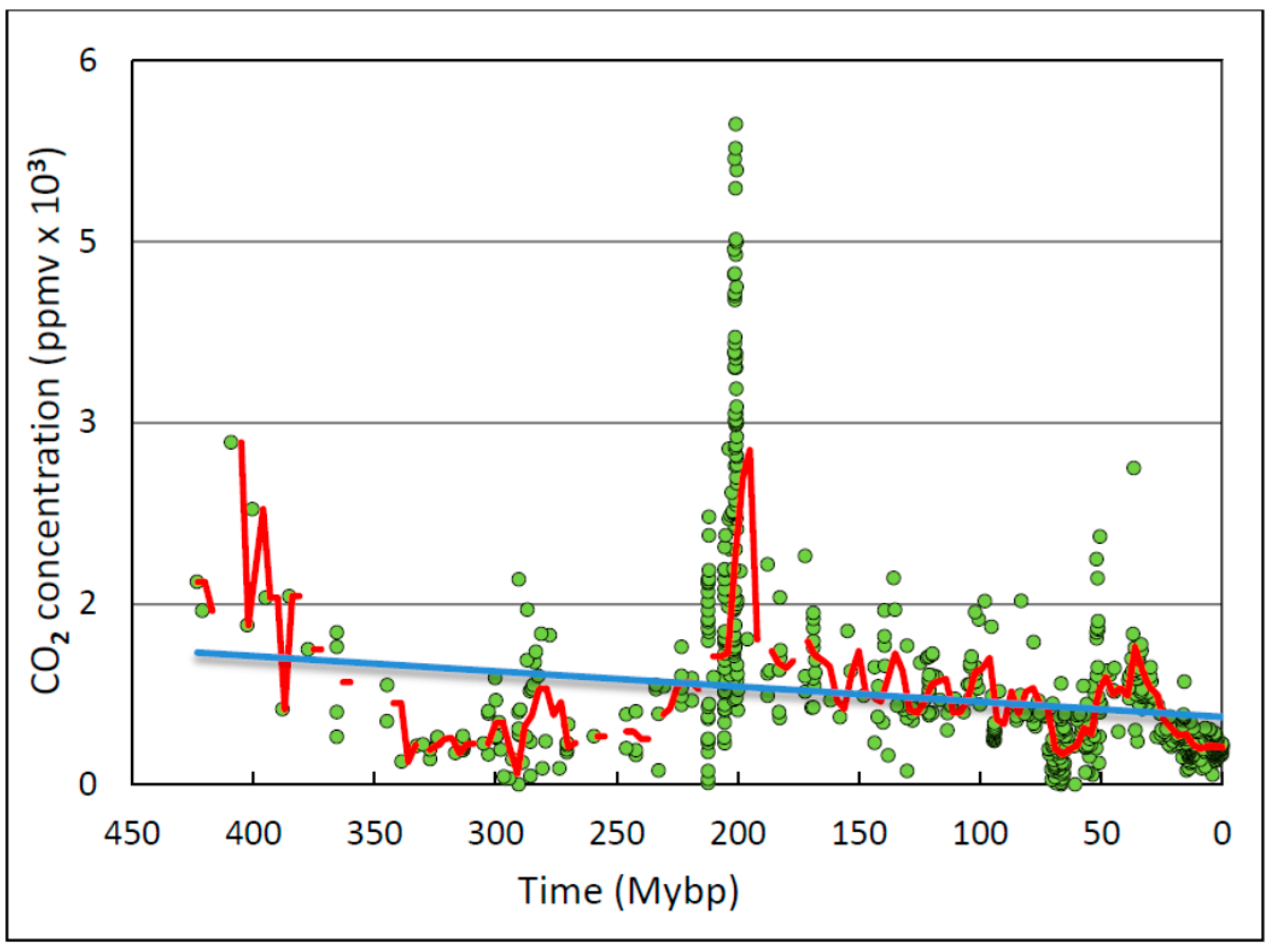
Figure 5.
Temperature (T) and atmospheric carbon dioxide (CO2) concentration proxies during the Phanerozoic Eon. Time series of the global temperature proxy (δ18O*(−1), red curve, n = 6680) are from Prokoph et al. [28] while concurrent atmospheric CO2 concentration proxies (green curve, n = 831) are from Royer [40]. The red curve plots moving averages of the non-detrended T proxy averaged in 50 My windows incremented in ten-My steps (the 10–50 My moving average in Figure 3b). The green curve shows mean CO2 concentration values in one-My bins averaged over high-resolution portions of the CO2 record (the most recent Phanerozoic) and linearly interpolated over low-resolution portions (the older Phanerozoic). Glaciations based on independent sedimentary evidence are designated by vertical blue cross-hatched areas, while putative cool periods are designated by vertical solid blue bars. Major cooling and warming cycles are shown by the colored bars across the top while geological periods and evolutionary milestones are shown across the bottom. Abbreviations: CO2, atmospheric concentration of carbon dioxide based on various proxies (Methods); ppmv, parts per million by volume; Silu, Silurian; Neo, Neogene; Quatern, Quaternary. The three major glacial periods and ten cooling periods identified by blue cross-hatches and solid lines, respectively, are (after [21]): Glacial periods. 1. late Devonian/early Carboniferous; 2. Permo-Carboniferous; 3. late Cenozoic. Cooling periods. 1. late Pliensbachian; 2. Bathonian; 3. late Callovian to mid-Oxfordian; 4. Tithonian to early Berriasian; 5. Aptian; 6. mid-Cenomanian; 7. mid-Turonian; 8. Campanian-Maastrichtian boundary; 9. mid-Maastrichtian; 10. late-Maastrichtian.
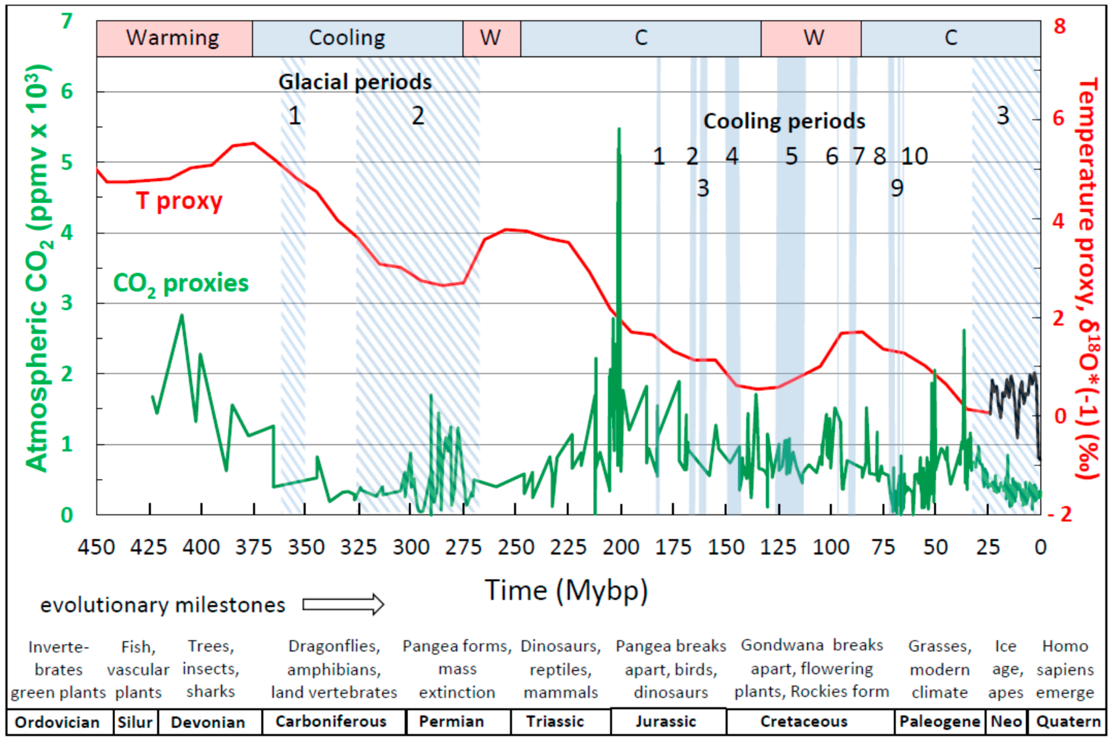
Figure 6.
Scatter plot of linearly-detrended temperature-proxy data averaged in one-My bins from 425 to 0 Mybp versus atmospheric carbon dioxide concentration. The negative correlation coefficient (R = −0.19, n = 206) is discernibly different from zero (p = 0.006) but weak (R2 = 0.036). The trendline was fitted by the method of least squares.
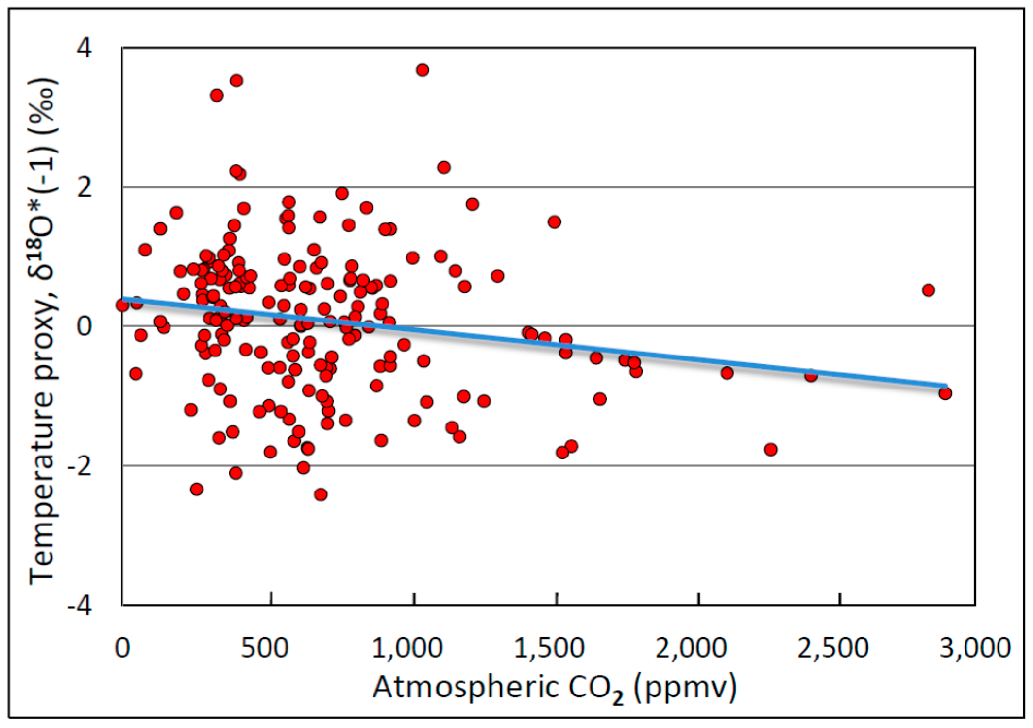
Figure 7.
Spectral power periodograms of atmospheric CO2 and temperature over the Phanerozoic Eon. The green and red curves show CO2 and temperature spectral density profiles, respectively. The temperature periodogram was constructed using detrended temperature proxy data. Time periods covered and (in parentheses) Fisher’s Kappa and the corresponding probability that the atmospheric CO2 concentration and T periodograms result from white (Gaussian) noise are 85 to 0 My (12.57, 1.96 × 10⁻⁵) and 522 to 0 My (28.98, 2.0 × 10⁻¹³), respectively.
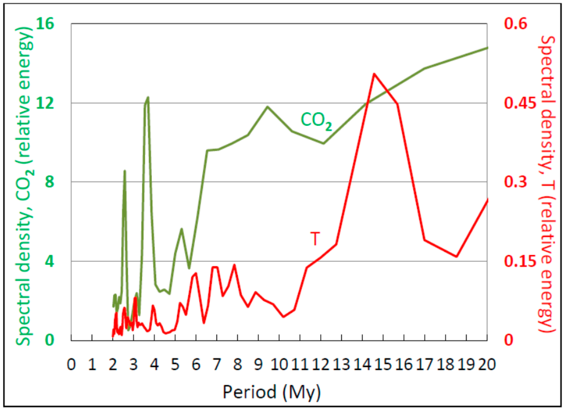
Figure 8.
Relationship among atmospheric CO2 concentration, radiative forcing (RF) and marginal radiative forcing (ΔRFCO2) computed using MODTRAN. Each graph shows a family of curves for three latitudes (key in (b)) and two cloud conditions (labeled only for the top pair of red curves in (a)). For each latitude the upper curve pertains to a cloudless sky and the lower curve to a cloudy sky containing cumulus clouds starting a base at 0.66 km and a top of 2.7 km. Remaining model parameters used to generate curves are described in the text. (a) Atmospheric CO2 concentration versus RF at the tropopause. (b) Difference analysis of the curves in (a) to show marginal radiative forcing (ΔRFCO2), i.e., the change in forcing associated with a unit increment in atmospheric CO2. Colored curves are in all cases computed from MODTRAN while the dashed black curves are best-fit logarithmic (a) or power function trendlines (b). Abbreviations: ppmv, parts per million by volume; W/m2, Watts per square meter. The arrow identifies the reference curve used for computing ΔRFCO2 decay constants because it most closely approximates values for the International Standard Atmosphere (see text).

Figure 9.
Scatter plot of detrended temperature-proxy data averaged in one-My bins from 425 to 0 My ago versus marginal RF by atmospheric CO2. The positive correlation coefficient (R = 0.16, n = 199) is discernibly different from zero (p = 0.02) at this large sample size, but weak, i.e., as ΔRFCO2 increased, the temperature proxy δ18O*(−1) increased only slightly. The trendline was fitted by the method of least squares.
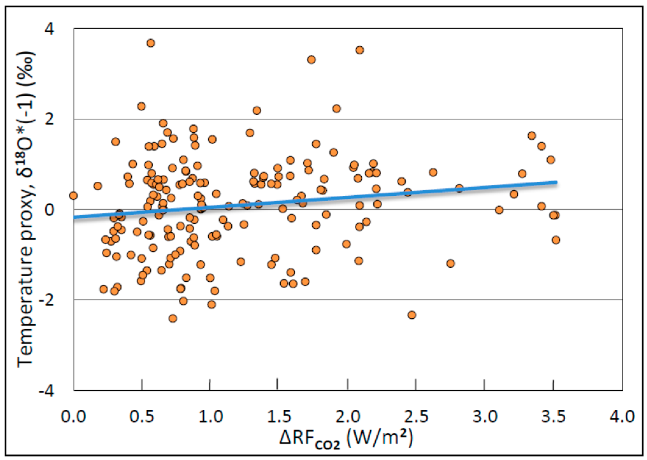
Figure 10.
Spectral power periodograms of ΔRFCO2 and T in the Phanerozoic climate. The orange and red curves show ΔRFCO2 and T spectral density profiles, respectively. The temperature periodogram was constructed using linearly-detrended proxy data. Time periods covered and (in parentheses) Fisher’s Kappa and the corresponding probability that the atmospheric CO2 concentration and T periodograms result from white (Gaussian) noise are 85 to 0 My (8.26, 0.005) and 522 to 0 My (28.98, 2 × 10⁻¹³), respectively.

Figure 11.
Time series of temperature proxies, atmospheric CO2 concentration and ΔRFCO2 over the Phanerozoic Eon. Purple arrows correspond to peaks in the strontium ratio determined independently from visual inspection of time series in [28]. Temperature proxies (red curve) are from Prokoph et al. [28]. CO2 proxies (green curve) are from Royer [40], represented here using a 3–6 My moving average. Yellow double-headed arrows highlight the expected antiphasic relationship between atmospheric CO2 concentration and marginal forcing computed for tropical latitudes under clear-sky conditions. The scale for the temperature proxy is modified here by a constant offset for graphical presentation on the same scales as the other proxies. The correct temperature-proxy scale is shown in Figure 5. In this and following graphs, climate variables are color-coded: red represents the temperature proxy, δ18O*(−1); green represents atmospheric CO2 concentration proxies converted to ppmv; and orange represents the marginal forcing calculated for each atmospheric CO2 concentration datapoint using the best-fit power function equation corresponding to the empirical curve for tropical latitudes under clear-sky conditions (Figure 8b).

Figure 12.
Lagged (serial) autocorrelation coefficient, R, of time series of Phanerozoic climate variables over the time period from 174 to 0 Mybp. The periodicity in the autocorrelation profiles demonstrates non-random periodicity in the corresponding climate variables. (a) δ18O*(−1). Average cycle duration, 22.4 My. (b) Atmospheric CO2 concentration. Average short cycle, 16.9 My. Average long cycle, 66.8 My. (c) ΔRFCO2. Average short cycle, 17.2 My. Average long cycle, 66.2 My. Double-headed arrows demarcate the approximate times of cycles and sub-cycles identified visually.

Figure 13.
As in Figure 12, but over the shorter time period from 174 to 87 Mybp. Average cycle durations: (a) 16.8 My (b) 18.0 My (c) 19.0 My. Otherwise as in the legend of Figure 12.

Figure 14.
Lagged (serial) cross-correlation coefficient, R, of temperature and atmospheric CO2 concentration proxies. (a) Time period from 174 to 0 Mybp. Average short cycle duration, 17.9 My. Average long cycle duration, 70.2 My. (b) Time period from 174 to 87 Mybp. Average short cycle duration, 15.4 My. Otherwise as in the legend of Figure 12.

Figure 15.
As in Figure 14, but for δ18O*(−1) and ΔRFCO2. (a) Time period from 174 to 0 Mybp. Average short and long cycle durations, 19.7 and 54.8 My respectively. (b) Time period from 174 to 87 Mybp. Average short cycle duration, 16.2 My. Otherwise as in the legend of Figure 12.

Figure 16.
As in Figure 14, but for atmospheric CO2 concentration and ΔRFCO2. (a) Time period from 174 to 0 Mybp. Average short and long cycle durations, 14.5 and 70.2 My respectively. (b) Time period from 174 to 87 Mybp. Average short cycle duration, 17.8 My. The strong negative correlation coefficients at low shift orders demonstrate the antiphasic (inverse) relation between atmospheric CO2 concentration and ΔRFCO2. Otherwise as in the legend of Figure 12.
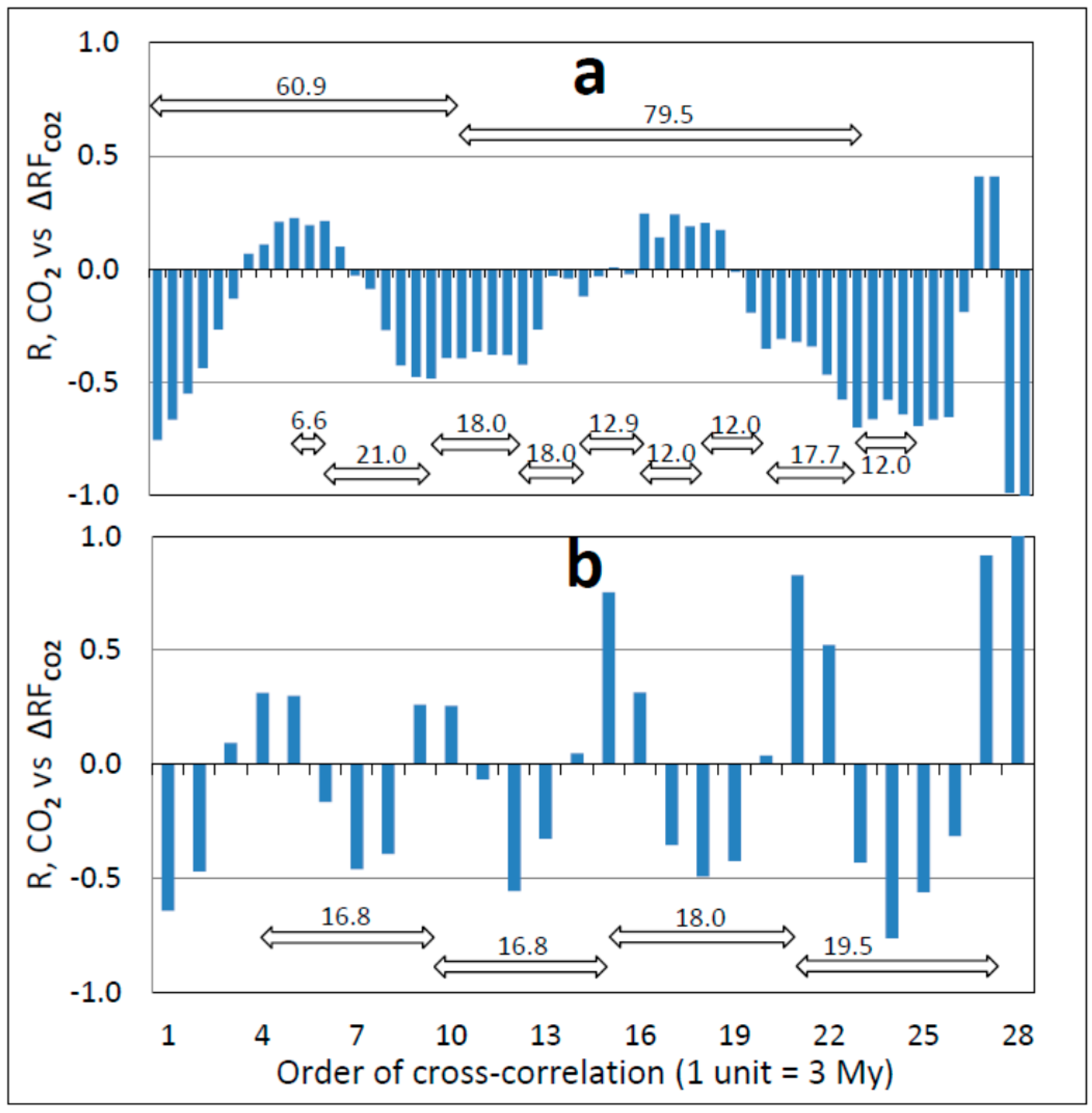

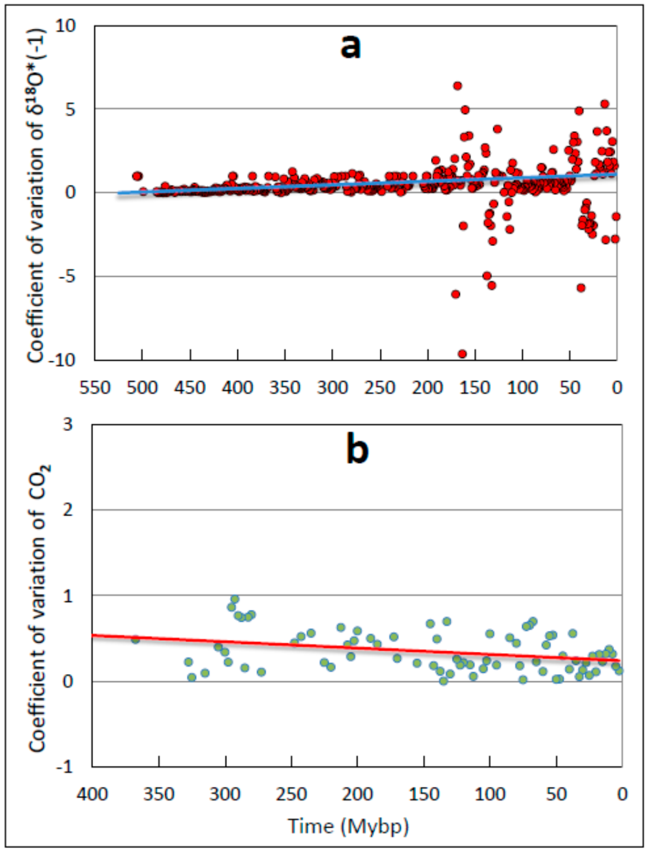
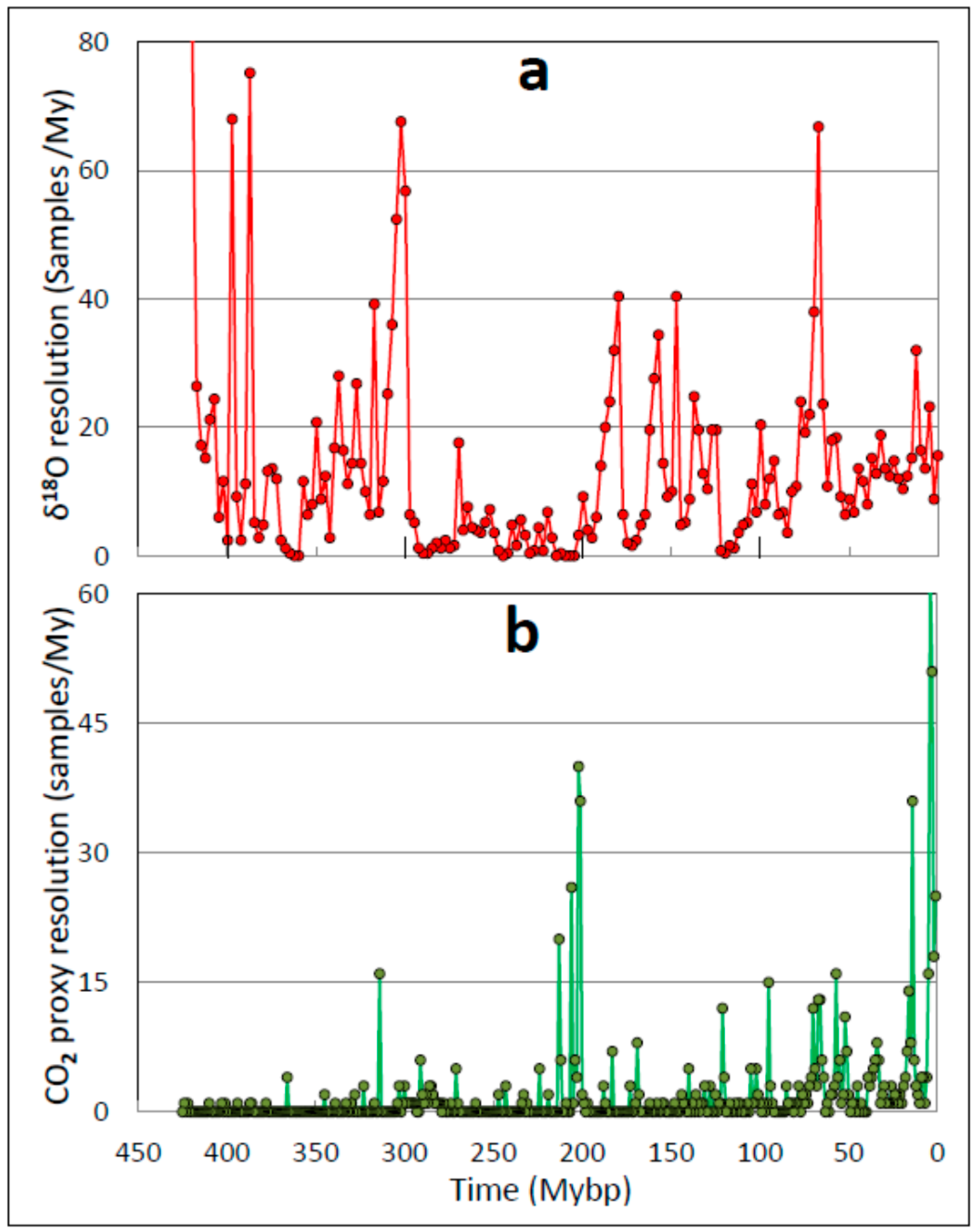
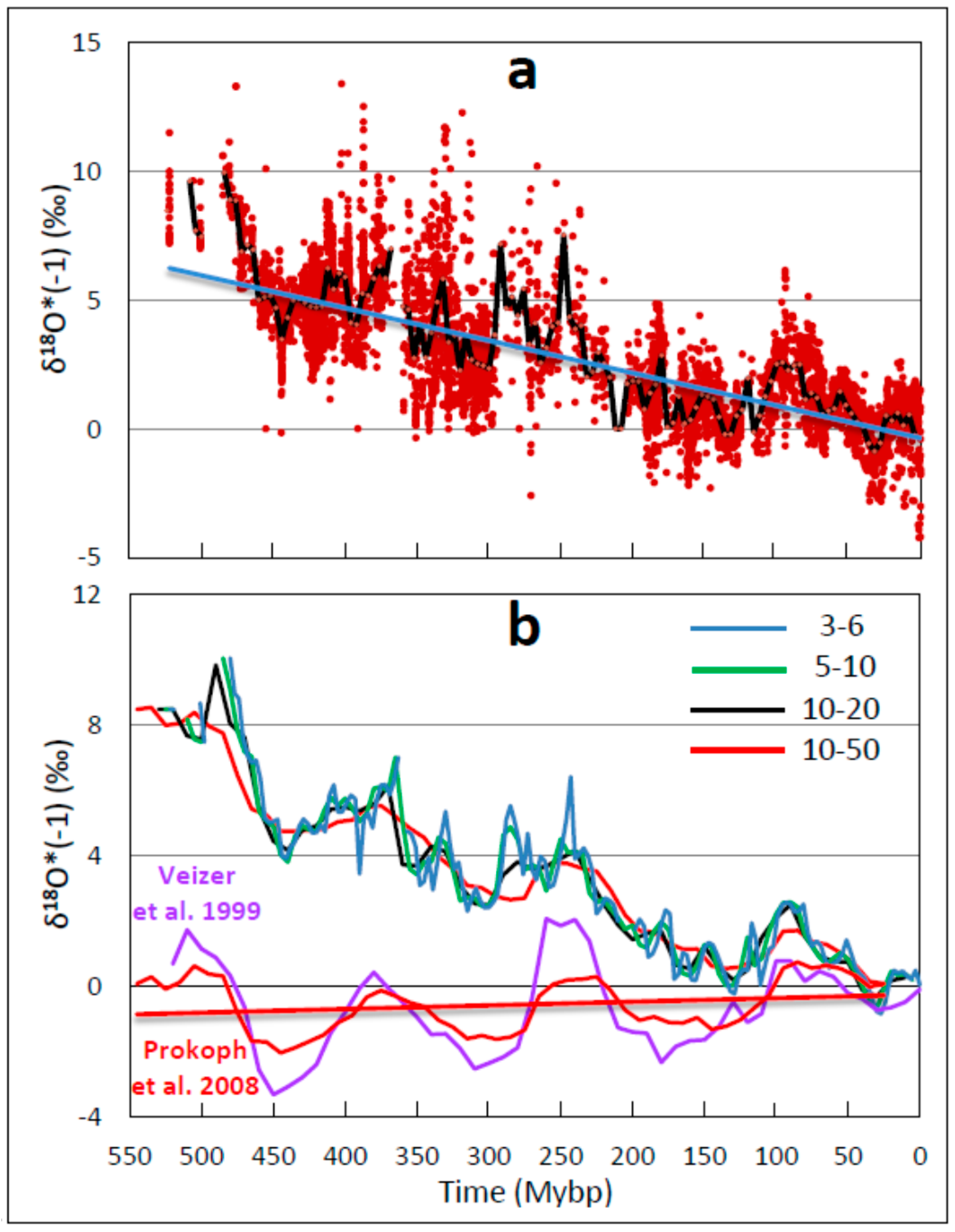
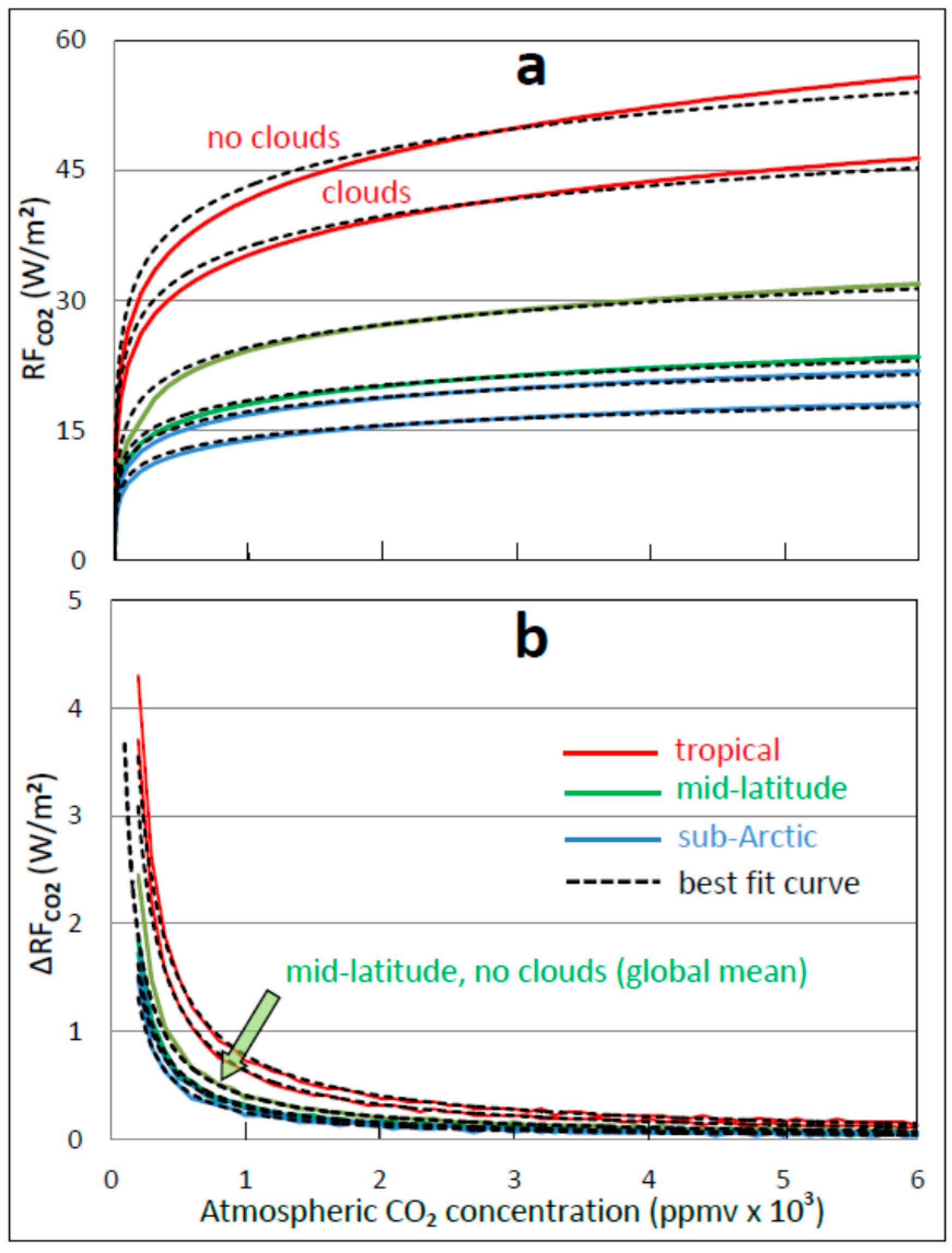
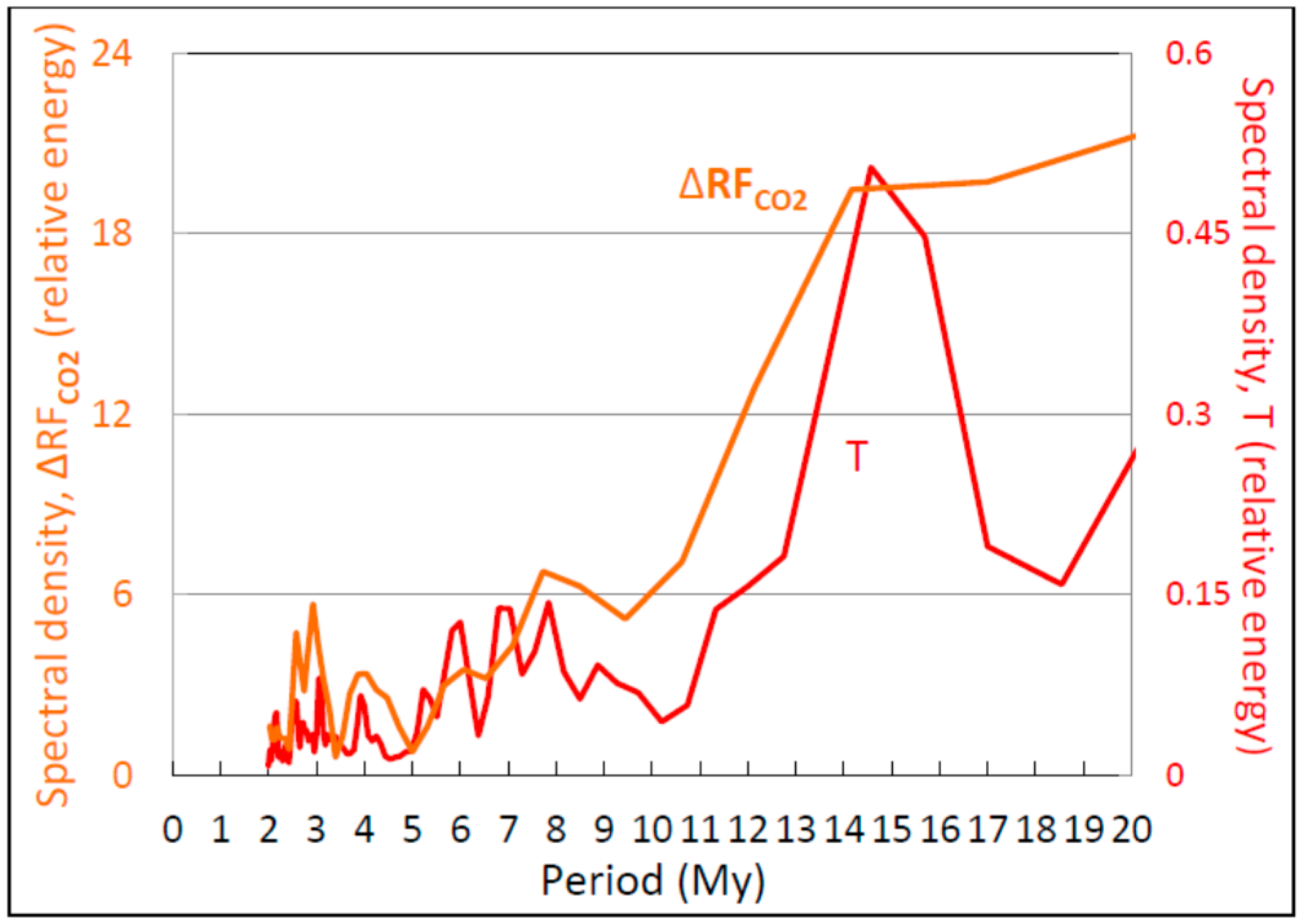
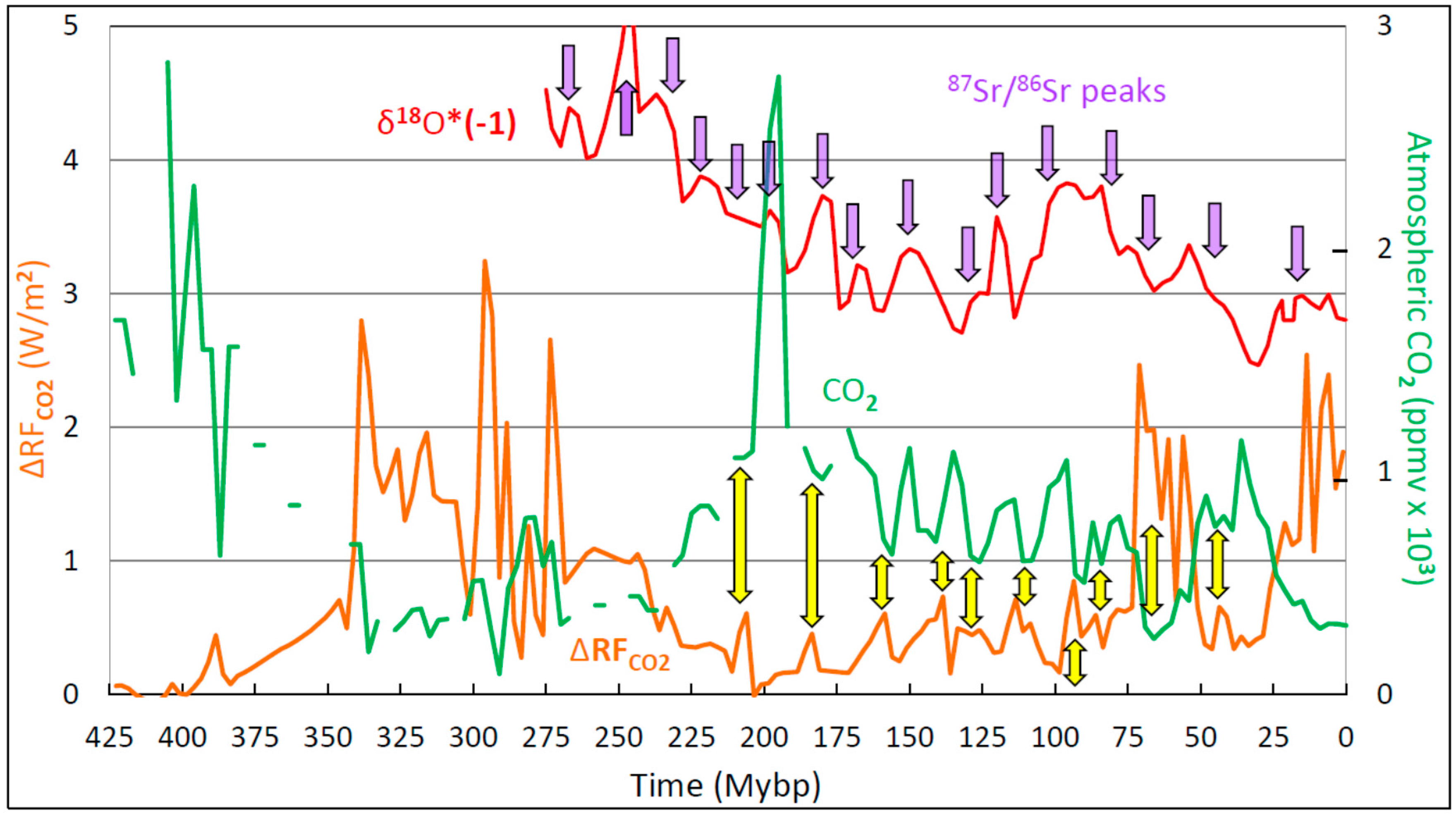
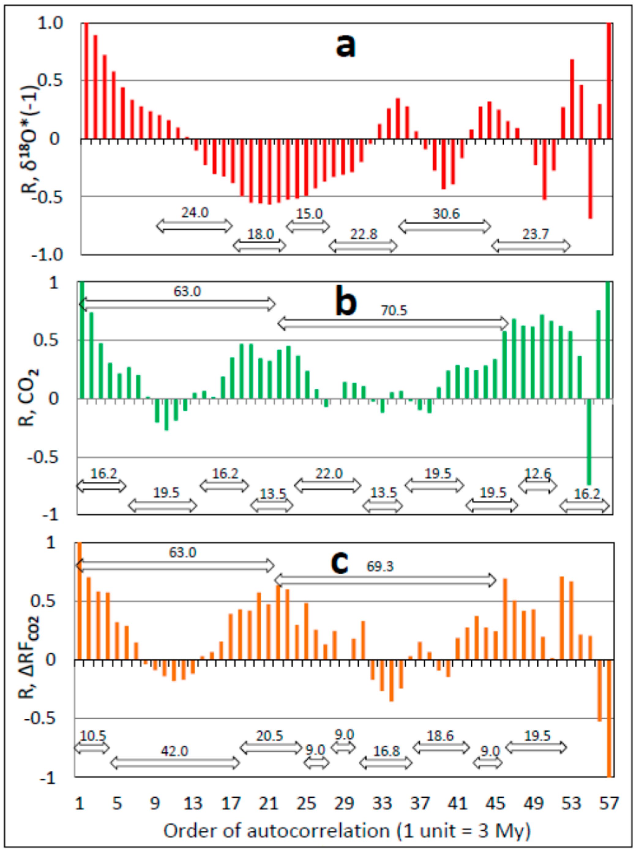
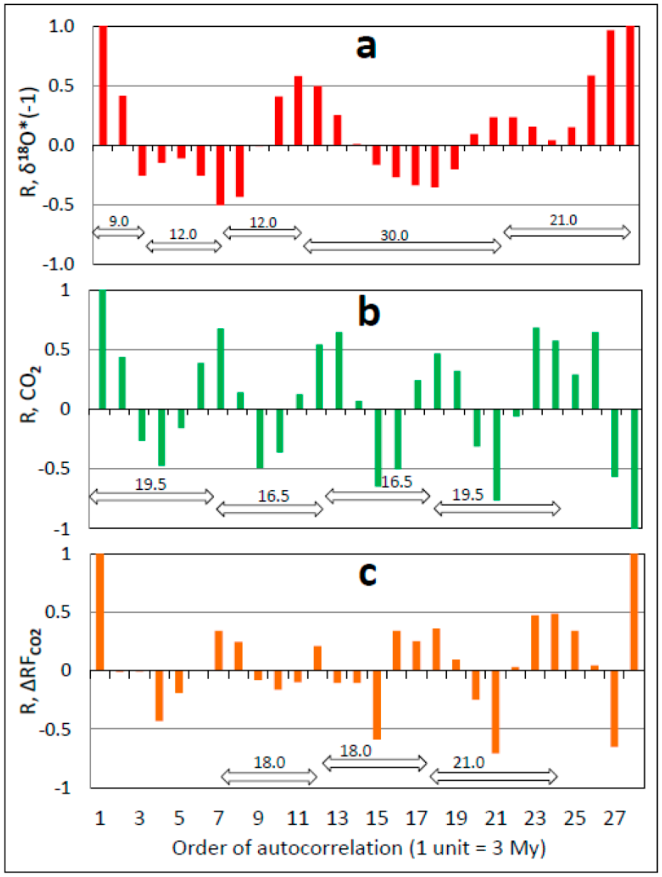
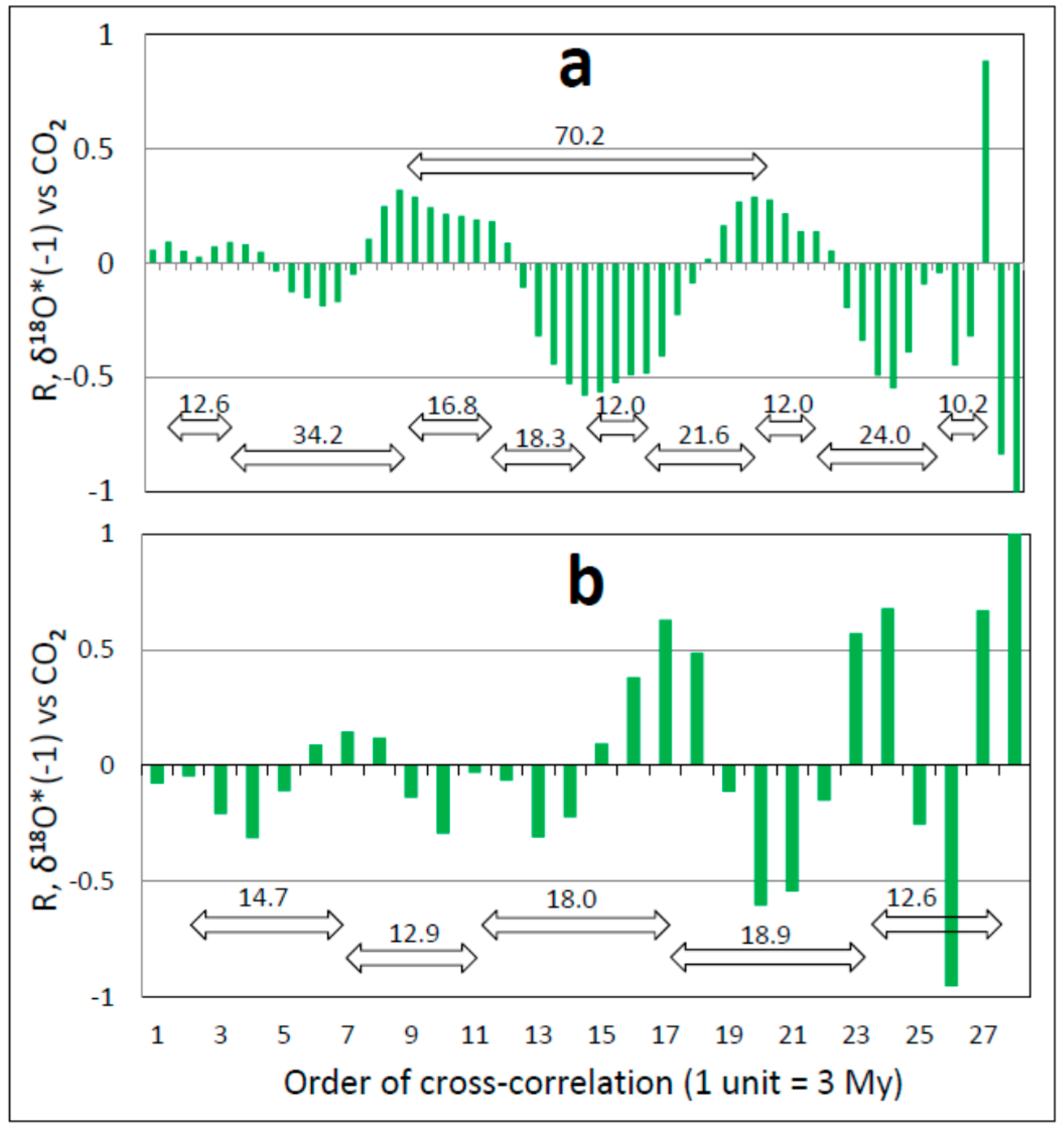
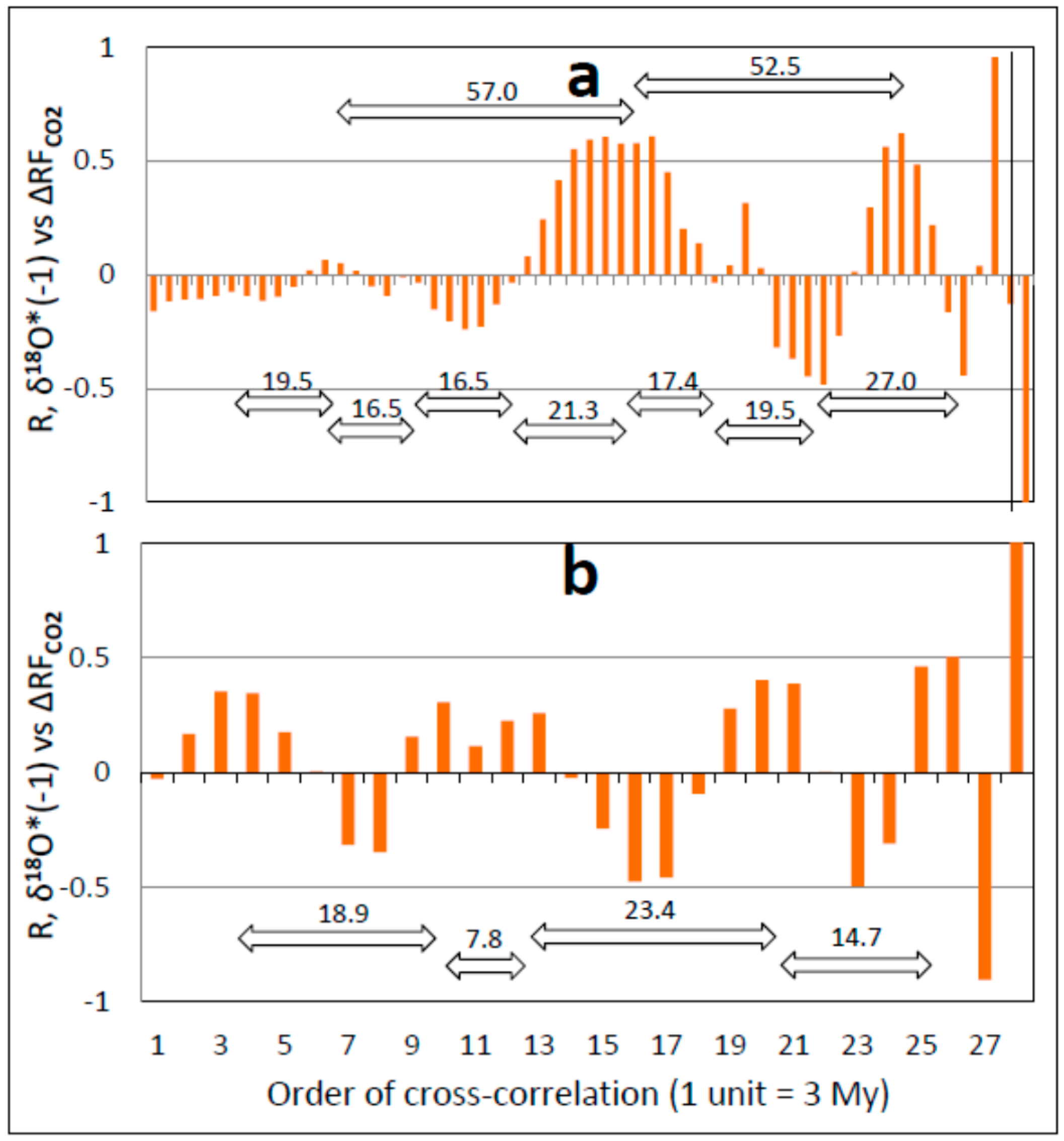
Table 1.
Correlation coefficients, temperature vs. atmospheric CO2 concentration (column D1) and temperature vs. marginal forcing (column D2) for the most recent (highest resolution) time periods of the Phanerozoic Eon.
Table 1.
Correlation coefficients, temperature vs. atmospheric CO2 concentration (column D1) and temperature vs. marginal forcing (column D2) for the most recent (highest resolution) time periods of the Phanerozoic Eon.
| A. Entry # | B. Time (Mybp) | C. Geological Periods and/or Description | D: R (n, p) | |
|---|---|---|---|---|
| D(1): CO2 v. T | D(2): ΔRFCO2 v. T | |||
| 1 | 71.6–69.6 | Campanian-Maastrichtian boundary | a N/A | a N/A |
| b N/A | b N/A | |||
| c 0.31 (19, 0.19) | c −0.31 (19, 0.20) | |||
| d −0.20 (11, 0.56) | d 0.02 (11, 0.96) | |||
| e −0.39 (11, 0.23) | e 0.39 (11, 0.23) | |||
| 2 | 80–50 | bracketed Campanian-Maastrichtian boundary | a 0.16 (31, 0.40) | a −0.06 (31, 0.75) |
| b 0.16 (31, 0.38) | b −0.05 (31, 0.80) | |||
| a 0.17 (31, 0.35) | a −0.12 (31, 0.52) | |||
| b 0.19 (31, 0.31) | b −0.12 (31, 0.52) | |||
| d 0.03 (110, 0.78) | d −0.13 (110, 0.19) | |||
| e −0.006 (110, 0.95) | e 0.03 (110, 0.72) | |||
| 3 | 67.5–66.5 | mid-Maastrichtian | a N/A | a N/A |
| b N/A | b N/A | |||
| c 0.09 (17, 0.92) | c −0.02 (17, 0.93) | |||
| d N/A | d N/A | |||
| e N/A | e N/A | |||
| 4 | 80–40 | bracketed mid-Maastrichtian | a −0.11 (41, 0.48) | a 0.14 (41, 0.37) |
| b 0.01 (41, 0.95) | b 0.06 (41, 0.70) | |||
| a −0.16 (41, 0.32) | a 0.10 (41, 0.55) | |||
| b 0.002 (41, 0.99) | b −0.03 (41, 0.84) | |||
| d −0.004 (116, 0.96) | d −0.12 (116, 0.20) | |||
| e −0.04 (116, 0.68) | e 0.05 (116. 0.59) | |||
| 5 | 0–34 | most recent global glaciation (late Cenozoic) | a −0.63 (34, 0.00005) | a 0.63 (34, 0.001) |
| b −0.73 (34, 0.00001) | b 0.53 (34, 0.00006) | |||
| a −0.48 (34, 0.0041) | a 0.52 (34, 0.002) | |||
| b −0.58 (34, 0.0003) | b 0.62 (34, 0.0001) | |||
| d −0.25 (179, 0.0006) | d 0.20 (179, 0.0075) | |||
| e −0.26 (179, 0.0005) | e 0.26 (179, 0.0005) | |||
| 6 | 0–26 | late Cenozoic, CO2 range similar to present | a 0.043 (26, 0.83) | a −0.02 ( 26, 0.94) |
| b −0.16 (26, 0.44) | b 0.16 (26, 0.42) | |||
| a −0. 052 (26, 0.80) | a 0.12 (26, 0.55) | |||
| b −0.16 (26, 0.44) | b 0.23 (26, 0.25) | |||
| d −0.03 (154, 0.70) | d 0.03 (154, 0.71) | |||
| e −0.05 (154, 0.53) | e 0.05 (154, 0.53) | |||
Red and black font designate discernible and non-discernible (p < 0.05, two-sided tests) Pearson product moment correlation coefficients (R), respectively. Green and blue fonts designate discernible and non-discernible Spearman Rho non-parametric (distribution free) correlation coefficients, respectively. The sample size and p value for discernibility are in parentheses immediately following each R value. The superscripts denote R calculated as follows: a. non-detrended temperature data averaged into one-My bins; b. linearly detrended temperature data averaged into one-My bins; c. non-detrended temperature data at the highest temporal resolution supported by the sampling frequency for the temperature-proxy database (see text); d. detrended temperature data with CO2 datapoints organized as matched pairs (see text); and e. Spearman Rho correlation coefficient for detrended temperature data with atmospheric CO2 concentration and T datapoints organized into matched pairs. The first column (Entry #) is included to facilitate cross referencing with the text. N/A designates non-applicable values owing to a sample size smaller than ten.
Table 2.
As in Table 1, but for the most ancient (lowest resolution) time periods of the Phanerozoic Eon.
Table 2.
As in Table 1, but for the most ancient (lowest resolution) time periods of the Phanerozoic Eon.
| A. Entry # | B. Time (Mybp) | C. Geological Periods Covered and/or Description | D: R (n, p) | |
|---|---|---|---|---|
| D(1): CO2 v. T | D(2): ΔRFCO2 v. T | |||
| 1 | 0–424 | most of Phanerozoic Eon | a 0.15 (191, 0.035) | a 0.10 (185, 0.16) |
| b −0.19 (206, 0.006) | b 0.16 (199, 0.02) | |||
| a −0.048 (191, 0.248) | a −0.037 (185, 0.61) | |||
| b −0.202 (191, 0.005) | b 0.193 (185, 0.0082) | |||
| 2 | 424–285 | first Phanerozoic temperature cycle (trough to trough) | a 0.22 (33, 0.23) | a −0.14 (35, 0.42) |
| b −0.16 (33, 0.37) | b 0.17 (35, 0.32) | |||
| a −0.04 (33, 0.86) | a 0.28 (33, 0.21) | |||
| b −0.095 (33, 0.61) | b 0.17 (33, 0.36) | |||
| 3 | 285–135 | second Phanerozoic temperature cycle (trough to trough) | a −0.17 (43, 0.26) | a 0.33 (39, 0.04) |
| b −0.16 (43, 0.30) | b 0.25 (39, 0.12) | |||
| a −0.14 (43, 0.36) | a 0.18 (39, 0.28) | |||
| b −0.22 (38, 0.10) | b 0.19 (38, 0.23) | |||
| 4 | 326–267 | Permo-Carboniferous glaciation | a 0.28 (22, 0.28) | a 0.03 (21, 0.90) |
| b 0.28 (22, 0.20) | b 0.05 (21, 0.82) | |||
| a 0.09 (22, 0.69) | a 0.26 (21, 0.25) | |||
| b −0.03 (20, 0.90) | b 0.26 (20, 0.27) | |||
| 5 | 400–200 | bracketed Permo-Carboniferous glaciation | a −0.30 (44, 0.05) | a 0.20 (42, 0.20) |
| b −0.17 (44, 0.26) | b 0.16 (42, 0.31) | |||
| a −0.22 (44, 0.16) | a 0.31 (42, 0.04) | |||
| b −0.12 (44, 0.44) | b 0.24 (42, 0.12) | |||
| 6 | 225–73 | Period of flat baseline with ~My ΔRF oscillations | a 0.15 (80, 0.17) | a −0.10 (70, 0.28) |
| b −0.11 ( 80, 0.25) | b −0.10 (77, 0.38) | |||
| a 0.23 (76, 0.042) | a −0.27 (72, 0.02) | |||
| b −0.03 (76, 0.79) | b −0.01 (70, 0.93) | |||
| 7 | 184–66.5 | early Jurassic to Cretaceous (brackets all cool periods) | a 0.15 (71, 0.11) | a −0.24 (68, 0.03) |
| b −0.01 (71, 0.09) | b −0.05 (68, 0.68) | |||
| a 0.20 (71, 0.09) | a −0.25 (68, 0.04) | |||
| b 0.02 (71, 0.88) | b −0.07 (68, 0.56) | |||
| 8 | 200–50 | bracketed early Jurassic to Cretaceous | a 0.21 (93, 0.02) | a −0.21 (89, 0.02) |
| b −0.11 (93, 0.30) | b −0.05 (89, 0.61) | |||
| a 0.25 (93, 0.02) | a −0.27, (89, 0.01) | |||
| b −0.10 (93, 0.33) | b 0.05 (89, 0.64) | |||
| 9 | 125–112 | Aptian | a 0.63 (12, 0.03) | a −0.71 (11, 0.01) |
| b 0.62 (12, 0.03) | b −0.70 (11, 0.02) | |||
| a 0.36 (12, 0.25) | a −0.26 (11, 0.43) | |||
| b 0.36 (12, 0.25) | b −0.27 (11, 0.41) | |||
| 10 | 140–80 | bracketed Aptian | a 0.12 (43, 0.43) | a −0.27 (41, 0.08) |
| b 0.11 (43, 0.43) | b −0.29 (41, 0.07) | |||
| a 0.17 (43, 0.25) | a −0.23 (41, 0.14) | |||
| b 0.15 (43, 0.35) | b −0.22 (41, 0.17) | |||
Conventions are the same as for Table 1 except that high-resolution data (subscripts c and d) and matched pair analyses (subscript e) are absent.
© 2017 by the author. Licensee MDPI, Basel, Switzerland. This article is an open access article distributed under the terms and conditions of the Creative Commons Attribution (CC BY) license (http://creativecommons.org/licenses/by/4.0/).
Share and Cite
MDPI and ACS Style
Davis, W.J. The Relationship between Atmospheric Carbon Dioxide Concentration and Global Temperature for the Last 425 Million Years. Climate 2017, 5, 76. https://doi.org/10.3390/cli5040076
AMA Style
Davis WJ. The Relationship between Atmospheric Carbon Dioxide Concentration and Global Temperature for the Last 425 Million Years. Climate. 2017; 5(4):76. https://doi.org/10.3390/cli5040076
Chicago/Turabian StyleDavis, W. Jackson. 2017. "The Relationship between Atmospheric Carbon Dioxide Concentration and Global Temperature for the Last 425 Million Years" Climate 5, no. 4: 76. https://doi.org/10.3390/cli5040076
Note that from the first issue of 2016, this journal uses article numbers instead of page numbers. See further details here.