Sky View Factor Calculation in Urban Context: Computational Performance and Accuracy Analysis of Two Open and Free GIS Tools


1
CNRS, UMR 6285 Vannes, France
2
Université de Bretagne Sud, UMR 6285 Vannes, France
*
Author to whom correspondence should be addressed.
†
These authors contributed equally to this work.
Climate 2018, 6(3), 60; https://doi.org/10.3390/cli6030060
Submission received: 31 May 2018
/
Revised: 24 June 2018
/
Accepted: 2 July 2018
/
Published: 4 July 2018
(This article belongs to the Special Issue Urban Overheating - Progress on Mitigation Science and Engineering Applications)
Abstract
:The sky view factor (SVF) has an important role in the analysis of the urban micro-climate. A new vector-based SVF calculation tool was implemented in a free and open source Geographic Information System named OrbisGIS. Its accuracy and computational performance are compared to the ones of an existing raster based algorithm used in SAGA-GIS. The study is performed on 72 urban blocks selected within the Paris commune territory. This sample has been chosen to represent the heterogeneity of nine of the ten Local Climate Zone built types. The effect of the algorithms’ input parameters (ray length, number of directions and grid resolution) is investigated. The combination minimizing the computation time and the SVF error is identified for SAGA-GIS and OrbisGIS algorithms. In both cases, the standard deviation of the block mean SVF estimate is about 0.03. A simple linear relationship having a high determination coefficient is also established between block mean SVF and the facade density fraction, confirming the results of previous research. This formula and the optimized combinations for the OrbisGIS and the SAGA-GIS algorithms are finally used to calculate the SVF of every urban block of the Paris commune.
1. Introduction
Urbanization is often characterized by a low vegetation density combined with a high fraction of impervious surfaces, a high rugosity (due to buildings’ size and height), and a denser energy consumption. These particular features affect the climate of the urban areas. Compared to the rural one, the urban microclimate shows a lower evaporation heat flux, a higher trapping of short and long-wave radiation, a lower ventilation and a larger amount of heat released in the atmosphere [1]. As a result, the temperature is often higher in urban areas than in its surrounding rural areas. This phenomenon is called Urban Heat Island (UHI) and may impact outdoor comfort [2], human health especially during heat waves [3], plant phenology [4], precipitation [5], energy consumption [6] and indirectly air pollution [7].
One of the climate change effects is the increase in the frequency and intensity of the heat waves, thus there is an urgent need to decrease the UHI phenomenon [8]. Several techniques have been investigated and tested all over the world: roof, facade and ground greening, roof and wall painting to alter the radiation absorption in both short and long-wave spectrum, water based solution such as fountains or sprinklers, building density and orientation optimization for shading purpose, etc. [9]. The performance of each technique may vary a lot both depending on the regional climate and the built environment where they are implemented. For example, Kikegawa et al. [10] showed that pavement watering was more adapted to residential areas than to narrow street canyons; Bernard et al. [11] have highlighted that the cooling induced by a given park would better propagate within streets having a large aspect ratio (building height to street width ratio—H/W); Ng et al. [12] have demonstrated that above a one-aspect ratio, the cooling benefit of a green roof at grade is low. To identify the best mitigation solutions adapted to a particular building environment, the efficiency of each solution may be tested running micro-climate models. Although this method is probably the most accurate, its applicability to each neighborhood of each city could be very expensive. Another solution is conceivable: based on a given set of climate-related parameters such as aspect ratio, albedo or vegetation density [1], each neighborhood may be classified in a specific built environment. Then, the efficiency of each mitigation solution may be tested running micro-climate models on a limited number of built environments, thus decreasing the number of simulations to perform for each city. In order to achieve such work, Stewart [13] proposed the concept of Local Climate Zone (LCZ): he defined ten built types and seven land-cover types based on a set of geometric and land-cover properties. These types and properties are detailed in Stewart and Oke [14]. One of the geometric properties, called Sky View Factor (SVF), defines the ratio of sky hemisphere visible from the ground (not obstructed by buildings, terrain or trees). This parameter is of major importance for urban climate applications since the long-wave radiation term is directly impacted by its value: the higher the SVF, the lower the long-wave radiation flux emitted by built surfaces to the sky during night-time. Oke [15] showed that the net long-wave radiation received on a given point located on the floor of a canyon is almost linearly related to the SVF of the point. At block scale (elementary area resulting from the division of the territory by the road network), Bernabé et al. [16] also showed a linear relationship (R² = 0.939) between the block mean SVF (the building roof and facades as well the ground surfaces were meshed in 10 m² triangles) and the net solar radiation. The SVF is then a very interesting parameter regarding urban climate applications. In order to obtain an accurate SVF value to each block of a city, it should be calculated for a high number of points. However, its calculation being computationally costly, it has been only performed on a limited sample of points for several years. This problem was partly solved for street canyons using an analytical solution [15]: the SVF of the mid-width of the floor of a canyon with symmetric cross-section and infinite length can be calculated using the Equation (1):
where is the canyon aspect ratio defined as the building height (H) divided by the street width (W).
Another solution to quickly calculate an approximate value of the block mean SVF is to use an empirical relationship with explaining variables being simple indicators calculated at block level. Bernabé et al. [16] found a linear relationship (R² = 0.8) between the block mean SVF and the block facade density fraction (defined Equation (2)):
where the area of free external facade (m²), and is the area of the urban block (m²).
However, these methods have not been largely used for LCZ classification yet since they have major limitations:
- the analytical solution is only adapted for urban canyons having an infinite length, which is rarely the case in real urban tissues. Moreover, when averaged at block scale, the is underestimated since it is only calculated at the center of the street.
- Concerning the empirical method, the relationship proposed by Bernabé et al. [16] is not valid for the SVF as defined in the LCZ properties. Bernabé et al. [16] calculated the SVF averaged to all urban surfaces (roofs, facades and ground), whereas, in the LCZ classification, it should only be averaged to ground surfaces.
- Last but not least, these methods are not adapted to all complexes urban tissues: the estimated SVF for some of them can be far from the real SVF value.
Several algorithms have been developed to calculate the SVF at any space position. Some of them use images (fish-eye, street view, etc.) as input data [17,18,19], and the others use either raster or vector data to identify the location of the sky obstacles [17,18,20,21,22,23]. The accuracy of the SVF values depends on the quality of the input data, on the method chosen and the value of its associated parameters (for example, the number of meshes of the sky hemisphere in the case of a ray throwing method). In these studies, the performance of the existing algorithms has been evaluated at point scale but never when averaged at block scale, while this information is of major importance for LCZ classification. Hämmerle et al. [17] selected several LCZ within the city of Szeged (Hungary), but they did not present their results through this variable. The objective of this work is then to evaluate the ability of two algorithms to accurately (and in a minimum computational time) estimate the SVF of a block independently of its LCZ type. In addition, the influence of the input data (raster or vector) used by the algorithm on the resulting SVF is also investigated.
The results of this work are addressed to any researcher or urban planner willing to apply a LCZ classification. Thus, the choice was made to use two SVF algorithms developed within two different free and open source GIS. The first is embedded in the software SAGA-GIS [24] and is also available as a plugin in QGIS. SAGA-GIS has the advantage of being known again and is often used by the urban climate community—for instance, in the framework of the World Urban DataBase and Access Portal Tools—WUDAPT (http://www.wudapt.org/—accessed in April 2018). Its algorithm is based on raster input data (information on building and terrain vertical elevation is stored in every pixel of the raster) and calculations are performed using two input parameters: the number of directions and the distance of search. The larger their value and the more accurate the SVF of each pixel, the longer it takes. The resolution of the raster is also a critical parameter both regarding accuracy and computational duration. It is a major limitation of the algorithm: since a building’s footprint is vector-based data, it has to be rasterized in order to be used in SAGA-GIS, thus inducing a loss of information proportional to the raster resolution. The second algorithm is based on vector data and has been developed within the OrbisGIS platform [25], which is also a free and open source GIS.
First, the effect of the algorithm input parameters (number of directions, search distance and grid resolution) on the SVF accuracy will be evaluated at point scale. Then, the block SVF accuracy and the processing time spent using each combination will be calculated. The results will be sorted by LCZ type in order to identify whether or not an algorithm is biased for any specific LCZ type. Finally, because the fastest method to calculate the SVF at block scale remains the use of morphological indicators, linear regression models will be used to test the intensity of their relationship with the block SVF.
2. Material
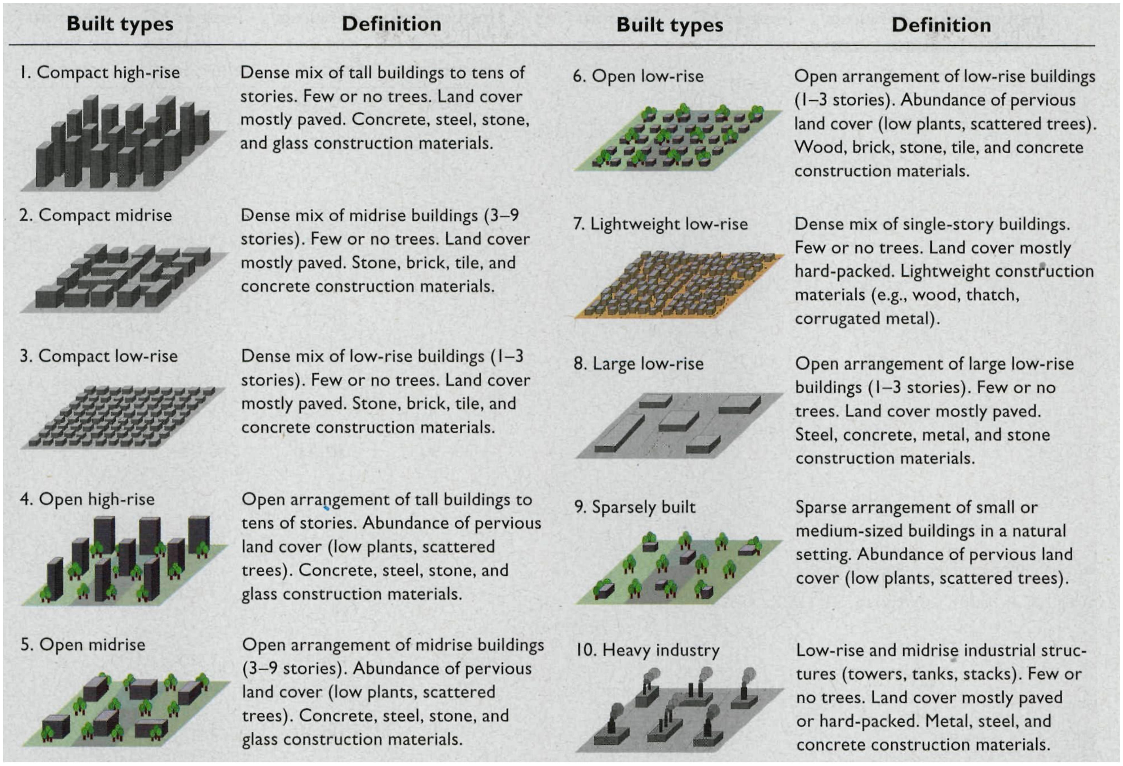
The dataset used to calculate the SVF in urban areas should contain the information concerning the location and the height of the following sky obstacles: trees, buildings and terrain. Except for some specific cities located in mountainous areas, the slope of the terrain is most of the time negligible compared to the angle created by a building seen from the street. On the contrary, trees may largely influence the SVF even in cities, but their influence fluctuates along the years because they grow, along the seasons because they lose their leaves (deciduous trees) and along each day because of the wind. For this reason and because trees also have very complex three-dimensional shapes, it is complicated to correctly represent them in geographical databases. This study is dedicated to the comparison of the accuracy and the time duration of SVF calculation method rather than to calculate accurately the SVF value of a given area. Thus, for the sake of simplicity, only buildings will be considered as sky obstacles. Depending on the buildings’ arrangement (distance between buildings and variability of this distance within a given area) and the buildings’ characteristics (building width, height, orientation and variability of these parameters within a given area), each algorithm could lead to more or less large errors when estimating the SVF. In order to identify the specific fail cases of each algorithm, they are tested on all LCZ built types (Figure 1).
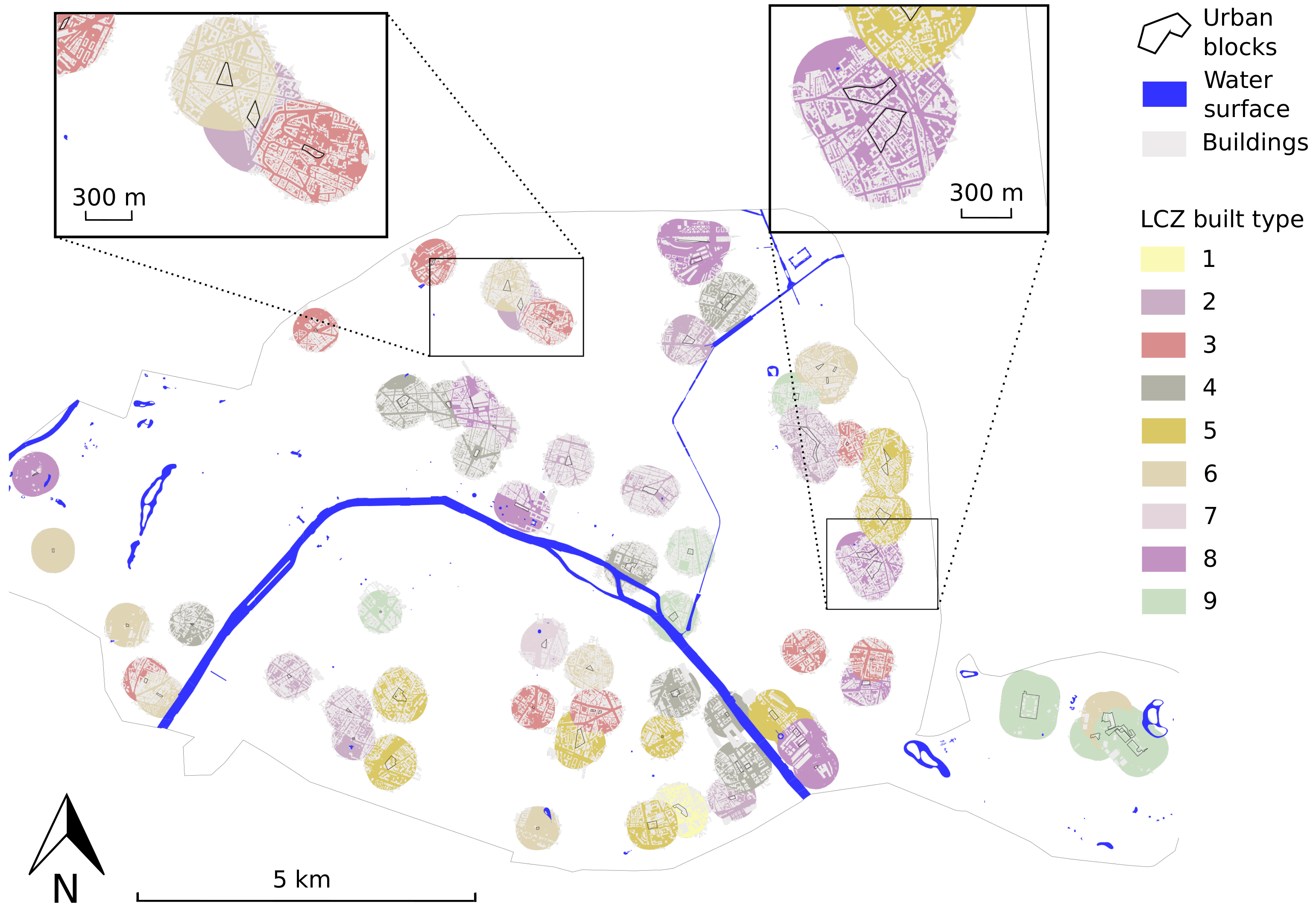
The Paris Region Urban and Environmental Agency IAUIdF (https://www.iau-idf.fr/en/about-us/who-we-are/a-foundation.html—accessed in April 2018) has manually attributed a LCZ type to each Urban Morphological Blocks (UMB) of the Paris region More information about the methodology used at http://www.iau-idf.fr/en/know-how/environment/vulnerability-of-towns-and-cities-to-rising-temperatures-assessed-using-the-local-climate-zones.html–accessed in April 2018. The boundaries of each UMB are built using a complex combination of data (road and rail networks, water surfaces and a land-use database [26], but they are most of the time very close to the urban block defined by the road network. In order to test the algorithms on each LCZ built type, ten urban blocks are randomly selected within the Paris commune for each LCZ type (except for LCZ 1, 7, 10 having, respectively, just 1, 1 and 0 individuals in the entire Paris territory). For the needs of this study, the buildings included within a 300 m radius around each urban block are conserved. The building data consist of the building footprint and height and they are provided by the French National Geographical Institute (more information about the data at http://professionnels.ign.fr/bdtopo—accessed in April 2018). The choice of the 300 m radius is based on preliminary results obtained by Chen et al. [23]: they showed that, in most of the cases, considering the buildings located further than 300 m from their calculation point does not bring much accuracy to the SVF calculation. Figure 2 shows the urban blocks and the buildings selected for the study.
3. Methodology
3.1. Presentation of the SVF Algorithm Used in OrbisGIS
The SVF is calculated from a given point considering all surrounding obstacles to the sky hemisphere. The points and obstacles are vector based data (geometries–polygons or lines) and should have vertical level information (three-dimensional geometry—if none, the level is considered to be 0 m from sea level).
For calculation purposes, the sky hemisphere is sliced into a given number of sectors (number of directions of analysis). A horizontal ray [R] of a given length is associated with each sector, starting from the center of the sphere and heading toward one of the sphere meridian confining the sector (Figure 3).
For each of the building obstacles encountered by the ray, the angle is calculated thanks to Equation (3):
where the height of the obstacle and the horizontal distance from the center of the sphere and the obstacle .
The highest angle made along the ray [R] is used to calculate the corresponding surface hemisphere hidden in this given direction (the sector is considered hidden all along its azimuthal angle—Figure 3). For a one meter radius sphere, is given by Equation (4):
where is the number of sky hemisphere sectors (number of ray directions)
The sky view factor is then calculated using Equation (5):
where d is a given azimuthal ray direction and is the surface of sky hemisphere hidden by obstacles in the azimuthal direction d.
Three input parameters are needed for the SVF calculation: the number of directions (number of sectors), the ray length and the ray step length (size of an elementary ray subdivision). and influence the processing time duration but also the accuracy of the calculation, whereas is only used to optimize the processing time duration. Indeed, the algorithm is based on the following procedure (simplified further details can be found on the function documentation page http://www.h2gis.org/docs/dev/STSVF/ and the source code is available at https://github.com/orbisgis/h2gis/blob/master/h2gis-functions/src/main/java/org/h2gis/functions/spatial/earth/STSvf.java—accessed in April 2018):
- for each ray (each direction);
- the ray is split into segments of 5 m length in order to optimize the calculation speed (according to a preliminary study, this parameter has very little effect on the calculation speed when its value is included within a (3–7) m range),
- the obstacles intersecting each of these segments are identified,
- for each intersection, the angle is calculated by means of Equation (3),
- the highest value encountered along the ray is conserved and used to calculate the corresponding sky hemisphere hidden in this direction (Equation (4)),
- the SVF is finally calculated subtracting the sum of the hidden surfaces in the directions to the total surface hemisphere (Equation (5)).
The SVF is implemented as a SQL function in H2GIS (the spatial database used by OrbisGIS to store and process GIS data [27]).
3.2. Global Methodology for Algorithm Evaluation
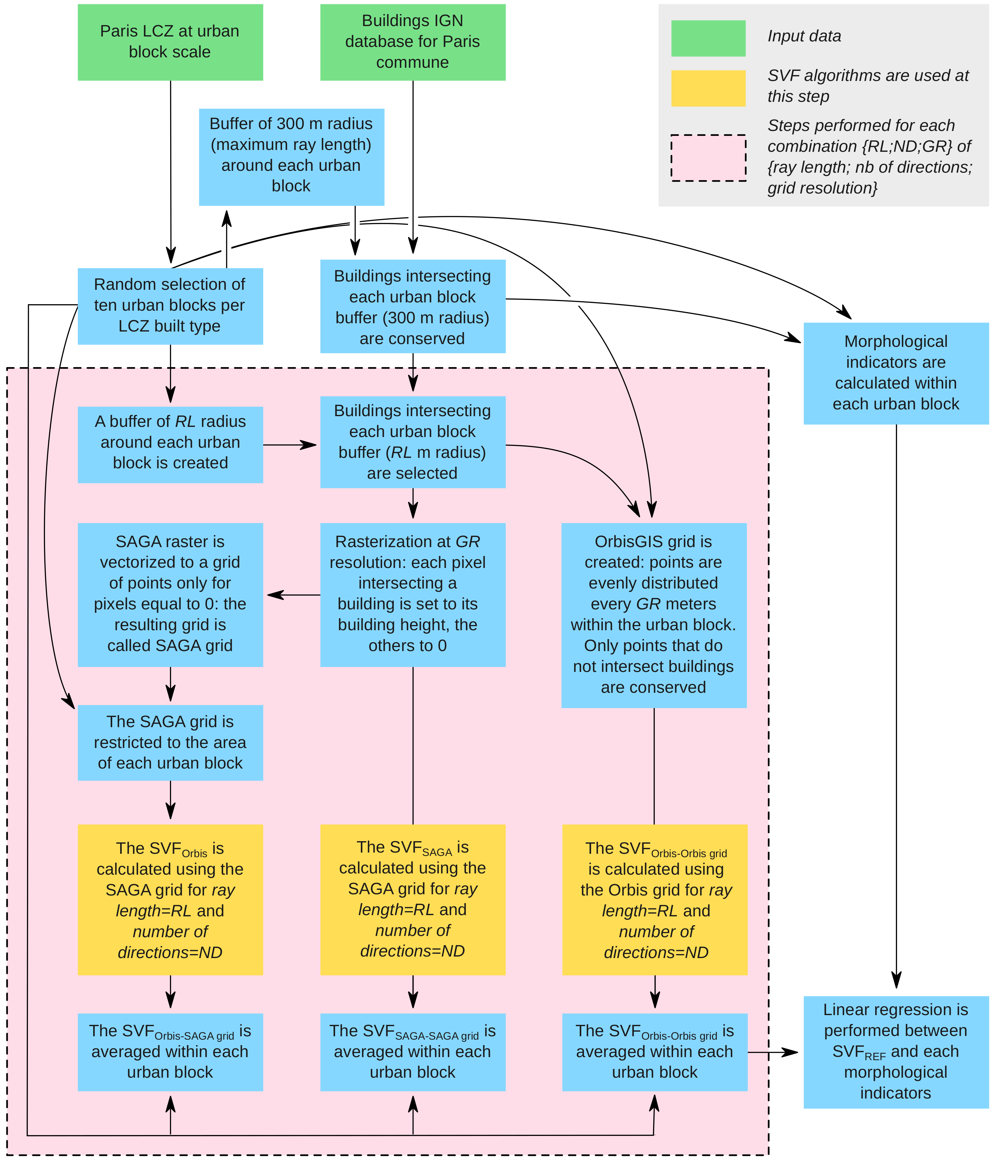
Figure 4 summarizes the global methodology used in the algorithm evaluation process.
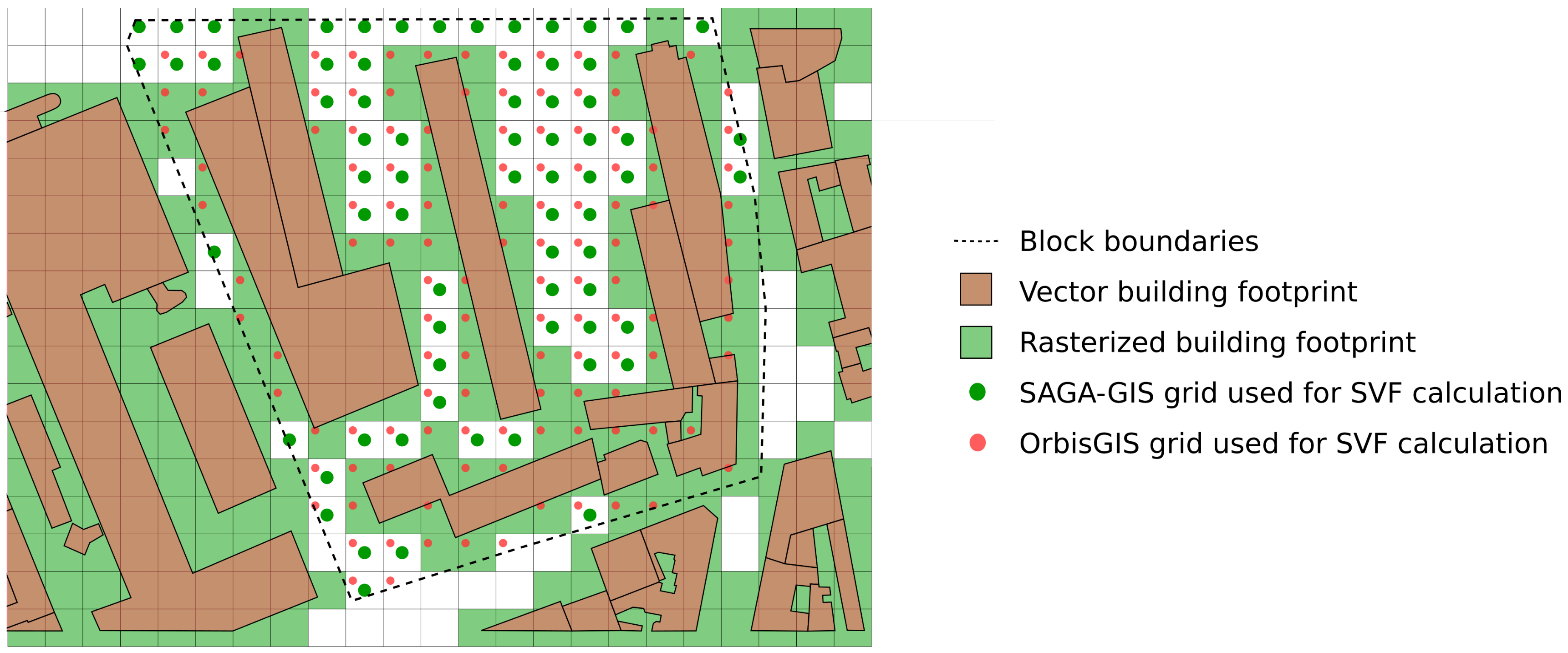
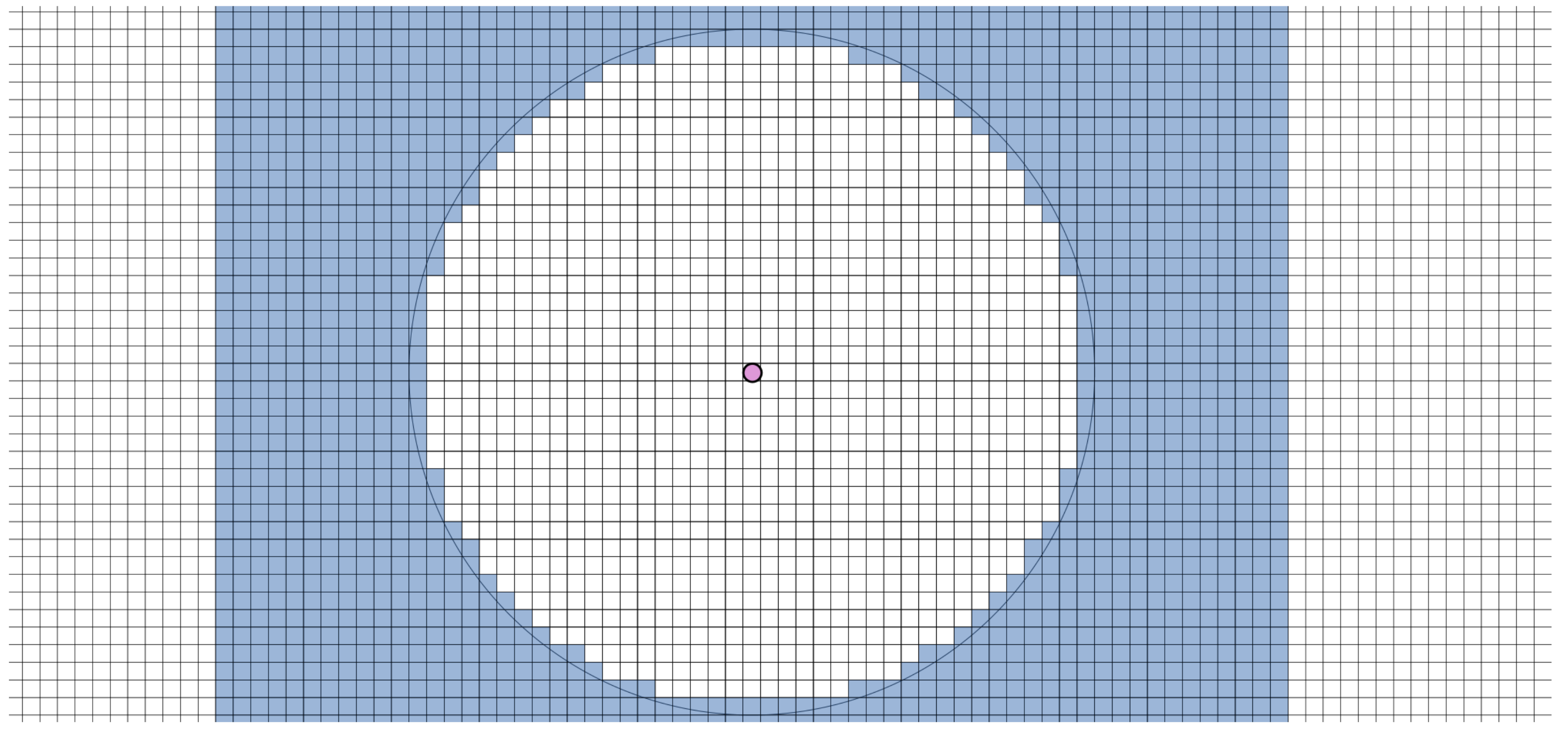
The algorithms are compared based on SVF values, both calculated at point and block scales. To compare points calculated by two algorithms one by one, there is a need to have the same set of points for SAGA-GIS and OrbisGIS. SAGA-GIS is more constrained by the buildings since they need a rasterization pre-process step: the value of a pixel partly covered by a building is set to its building height (cf. Figure 5—this is an arbitrary choice, the value could have been set to ground level whenever the building do not cover entirely the pixel). Then, since the SVF defined in the LCZ classification should be calculated at ground level, only the SAGA pixels that do not intersect buildings will be used. These pixels are vectorized to points, their value being attributed to their central point. The resulting grid of points is called SAGA-grid and is used by the OrbisGIS algorithm (Figure 4).
The SAGA-GIS grid is very constrained by the building location and may be biased by the rasterization process (no point can be closer to a building than half the grid resolution—Figure 5). For this reason, the OrbisGIS algorithm will also be used on a second grid called Orbis grid, which is not affected by the rasterization process. Figure 5 shows the differences between the SAGA-GIS grid and the OrbisGIS grid.
One of the objectives of this study is to identify what the input parameters values are in order to both minimize the algorithm processing time and to maximize its accuracy. The parameter values given in Table 1 will be tested.
The maximum values have been chosen based on Chen et al. [23] study. They calculated a SVF value for about a million of points in the city of Hong Kong testing different values for the ray length and the number of directions. Results showed that:
- when they compared values based on a 300 m ray length to the ones obtained with a 500 m ray length, the largest difference reported in their domain was just 0.031,
- no difference was reported in their domain when they used either 180 or 360 numbers of directions.
Thus, the maximum ray length has been set to 300 m and the number of directions to 180 (note that Gál et al. [28] chose for their calculations, respectively, 200 m and 360). Regarding the grid resolution, Chen et al. [23] set arbitrarily the value to 2 m since it is not a sensible parameter in their algorithm. We tested a finer resolution (1 m) to observe if it brings any improvement to the resulting SVF for the raster based algorithm.
3.3. Identification of the Reference Algorithm
The SVF value that will be taken as the reference at point or block scale should be the closest to the real SVF value.
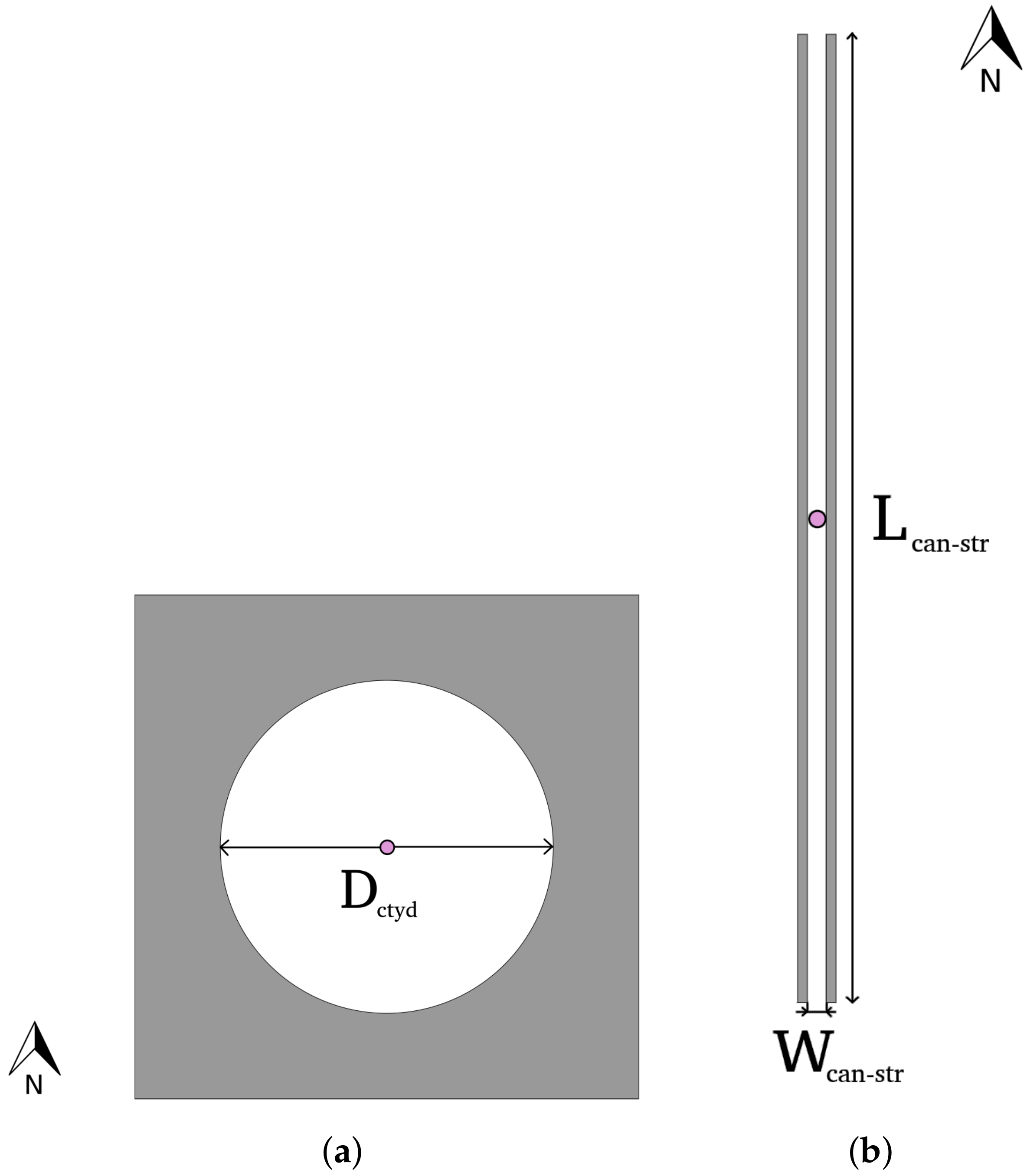
The accuracy of the two algorithms is tested at point scale setting their parameters at the finest resolution (the ray length is 300 m, the number of directions is 180 and grid resolution is 1 m). Two academic building configurations having an analytical solution for the SVF calculation are then used to test the accuracy of each algorithm. The first configuration is a square building extruded in the middle with a circular hole (Figure 6a). The SVF is then calculated from the centre of the courtyard and the analytical solution is given by Equation (6) [1]:
where is the SVF calculated at the center of the courtyard; is the height of the extruded building (m); and is the diameter of the circular courtyard (m).
The second configuration is an infinite street canyon (Figure 6b), the SVF being calculated at the middle of the street by means of the Equation (7) [15]:
where the SVF calculated at the middle of the street canyon, the building height of the street canyon (m), and the width of the street canyon (m).
Each configuration is stored in a geographical database and can be displayed in a GIS (Figure 6).
Two scenarios are proposed in order to test the effect of specific dimensions on the raster algorithm (Table 2).
The only difference between these scenarios concerns the horizontal distances. For the scenario 1, and are chosen in order to match the pixel boundaries and the building walls exactly, limiting the rasterization effect. In the second scenario, the buildings are shifted from half the grid resolution (0.5 m) in order to cover only partially some of the cells. In this way, the effect of the rasterization can be evaluated (each cell covered partially by buildings is transformed to a building cell). Note that, for both scenarios, the configurations do not exactly respect the ideal cases defined by [1,15]. However, we tried to limit the adverse aspects of the real cases. The courtyard of the extruded building is not a perfect circle, but it is defined by 720 points (four times the number of directions of the algorithms). The canyon street does not have an infinite length, but it is 2000 m long (longer than the ray length of the algorithm set to 300 m).
The accuracy of the SVF averaged at block scale depends on the accuracy of the SVF calculation at point scale, on the number and on the position of the points within the block. The accuracy at point level is evaluated using the scenarios described in Table 2, whereas the number and position of the points give a clear advantage to the vector approach due to the lack of flexibility induced by the raster based approach: the point position is constrained by the raster (points are equally distributed within the block). Moreover, the number of points will be limited since, in very dense built-up areas, most of the grid cells will be covered (even partially) by a building (see, for example, Figure 5). Consequently, except if the SAGA-GIS shows a higher accuracy at point level, the OrbisGIS grid and algorithm are selected to calculate the SVF value that will be used as a reference at block scale.
3.4. Empirical Relationship between Block Mean SVF and Morphological Indicators
Four morphological indicators are proposed to estimate the block mean SVF. They are calculated based on the building and the urban block (defined by the road network) geometries. Their definition and calculation method are given in Table 3.
The empirical model is built considering a simple linear relationship between the reference SVF calculated at block scale () and each of the morphological indicator (Equation (8)):
where is the regression intercept, and is the regression coefficient.
4. Results
4.1. Identification of the Reference Algorithm
The results of the analysis of SVF calculation at point scale shows a slight advantage of the OrbisGIS algorithm (Table 4).
The relative error of the OrbisGIS SVF is considered as negligible (always <0.01%) for any scenario and any configurations. Concerning the SAGA-GIS one, it is under 0.1% only for the circular courtyard case (configuration 1), when a given number of pixels constitutes the vertical or the horizontal building courtyard diameter (scenario 1—cf. Figure 7).
For this pixel resolution (1 m) and whenever the buildings do not exactly cover the raster pixels, the OrbisGIS algorithm seems to be more accurate than the SAGA-GIS one. Thus, for a given combination of ray length/number of direction, the SVF values obtained with the OrbisGIS algorithm will be considered as reference values.
As stated in Section 3.3, the SVF averaged at block scale will be more accurate when calculated using a vector-based approach rather than a raster-based approach. Therefore, the SVF calculated with OrbisGIS is considered as the reference at block scale for two reasons: the algorithm is based on a vector approach and the SVF calculated at point scale is more accurate than the SAGA-GIS one. The reference case used for block scale comparisons will then be the SVF calculated using the OrbisGIS algorithm, the OrbisGIS grid and with the following combination of parameter values: ray length equals to 300 m, number of direction equals to 180 and grid resolution equals to 1 m.
4.2. Effect of the Algorithm Input Parameters
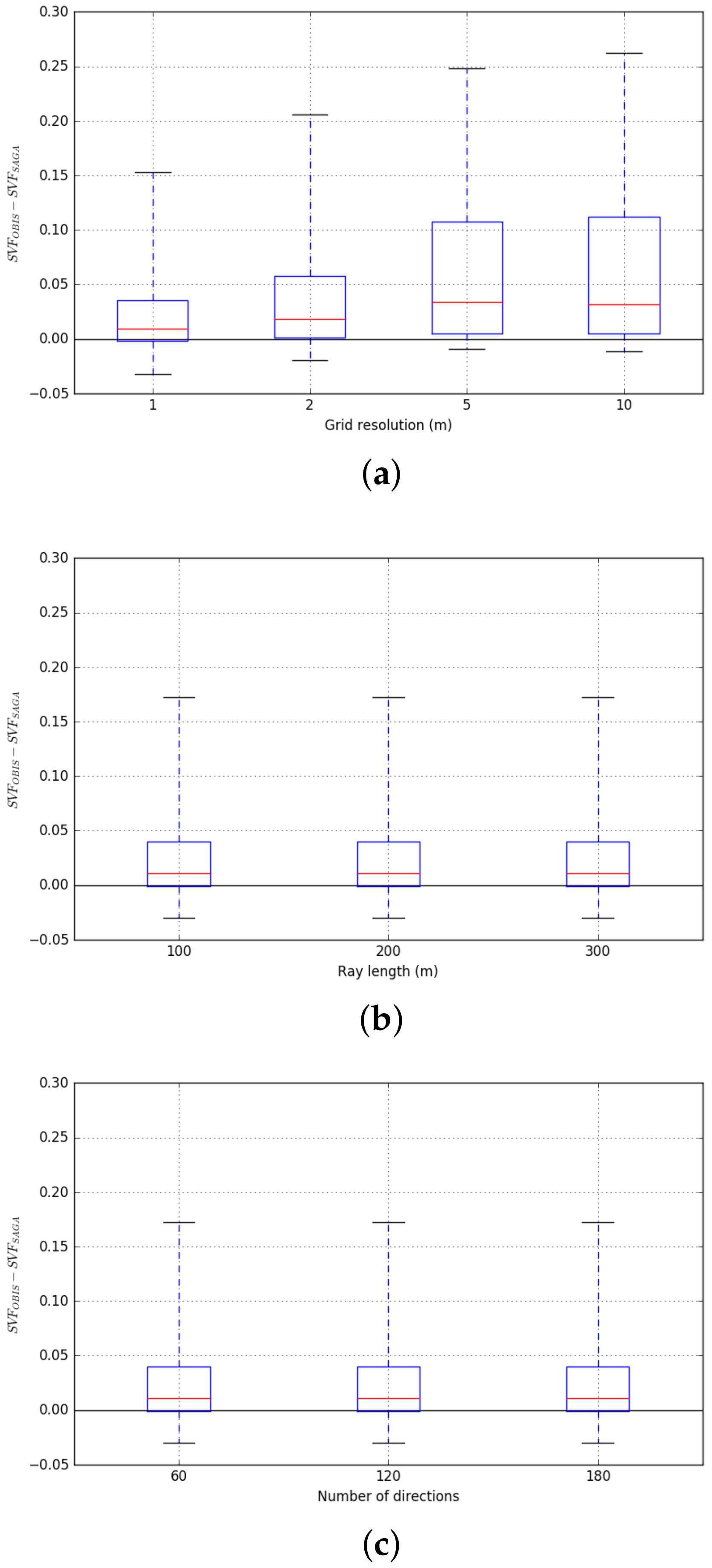
For each point of the SAGA-GIS grid, the SVF has been calculated using the OrbisGIS algorithm and the SAGA-GIS algorithm. The effect of the input parameters (ray length, number of directions and grid resolution) is then investigated subtracting for each point the SVF values calculated using SAGA-GIS to the one calculated using OrbisGIS. The analysis of the results shows that SVF values calculated using OrbisGIS are most of the time higher than the one calculated using SAGA-GIS (Figure 8). The effect of the grid resolution is of major importance: the larger the grid resolution, the higher the OrbisGIS to SAGA-GIS SVF difference (Figure 8a). The number of direction and the ray length seem to have a similar influence on the two algorithms since no change are highlighted by the modification of their values (Figure 8b,c).
The reason of the low SAGA SVF values results from the raster-based method, in particular from the method chosen for pixel value attribution. Figure 5 illustrates well the problem: as long as a building covers a part of a raster pixel, the entire pixel is considered as a building. Then, the buildings are closer to the calculated point in the SAGA-GIS case than in the OrbisGIS case, thus resulting in a lower SVF value. The intensity of this phenomenon is increased as the grid resolution increases.
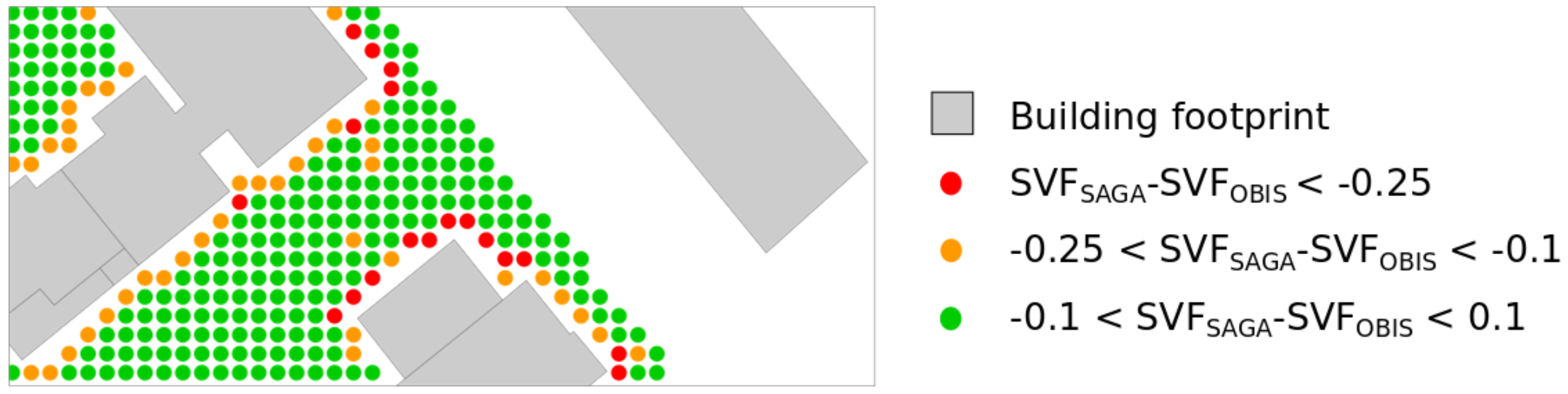
The SVF calculated using the two algorithms converges towards a same value when the grid resolution decreases. However, even for a 1 m grid resolution, it remains locally high for some points. The maximum observed is 0.65: the SAGA SVF value at this point is negative (−0.104), whereas the one calculated using OrbisGIS is 0.549. This value and most of the largest observed differences are located near the building walls (Figure 9). For such points, in the rasterization case, the relative error of distance between the point and the wall could be very high. This phenomenon is especially exacerbated when a point is located near a building corner facing one of the four cardinal points. Therefore, more investigation is needed to understand the reason of the negative values obtained with the SAGA-GIS software.
4.3. Ideal Input Parameters for Block Mean SVF Calculation
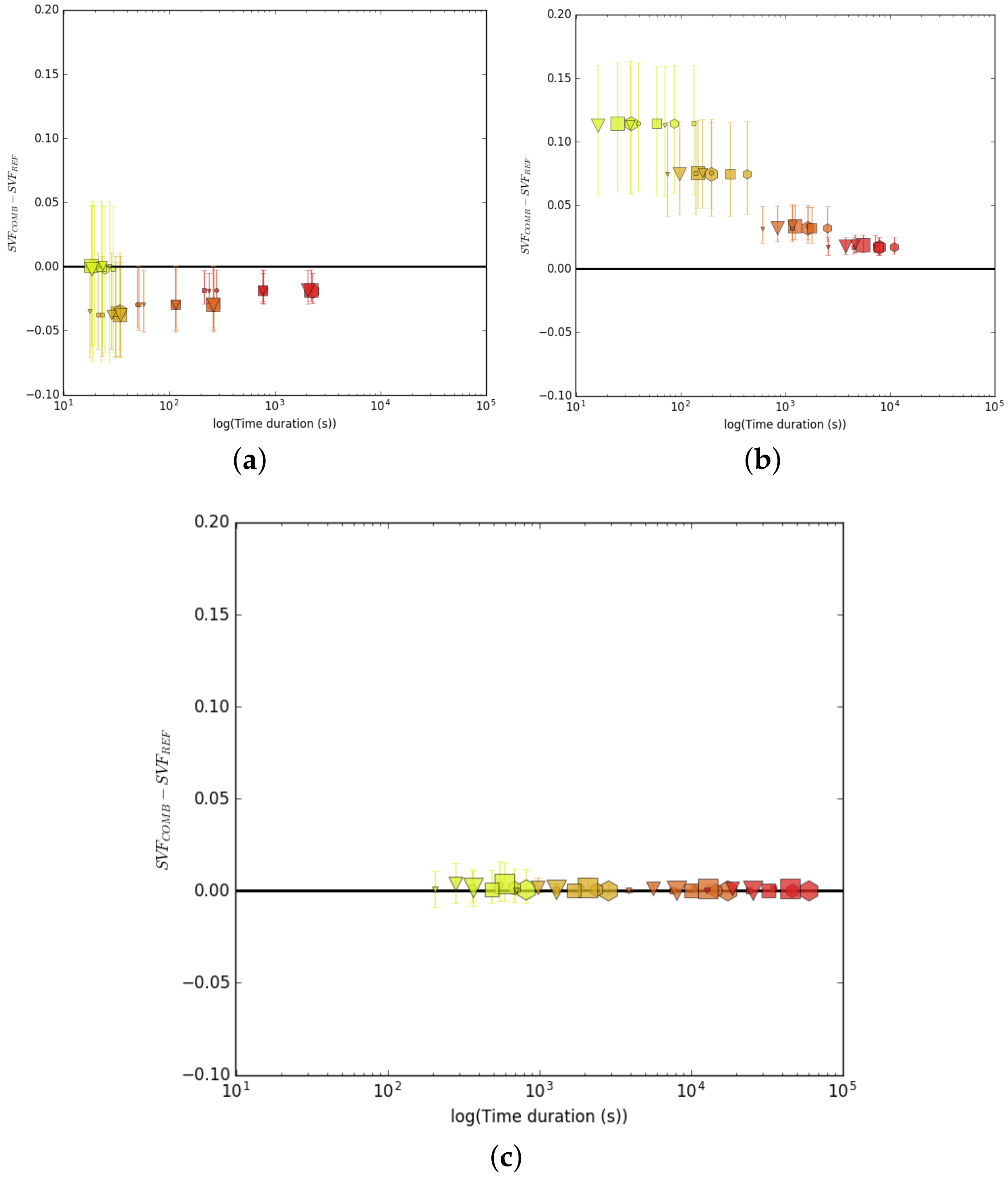
The block mean SVF has been calculated for each combination of RL, ND, GR, algorithm and grid. The computation duration of each combination has been measured. The error is defined as the difference between the block SVF calculated using a given combination and the one calculated using the reference combination (300 m, 180, 1 m, OrbisGIS, OBIS grid). The combination both minimizing the error and computational duration is identified in Figure 10.
Concerning time duration, the SAGA algorithm seems to be more impacted by the grid resolution and the ray length change rather than by the number of directions (Figure 10a). On the contrary, all parameters almost equally affect the OrbisGIS performance (Figure 10b,c). The time duration comparison will be further investigated in the discussion section.
Concerning the SVF error, three distincts behaviours are identified. The SAGA error is almost null for the theoretically worst combination of input parameters, it becomes negative when the combination is getting better and finally converges towards zero for the theoritically best combination. The Orbis/SAGA (OrbisGIS algorithm using SAGA grid) values are always overestimated but the error converges toward zero as the resolution decreases. The Orbis/Orbis (OrbisGIS algorithm using OrbisGIS grid) error very quickly decreases to zero as the combination of input parameter is getting better. An interesting fact is that it seems impossible to lower the error under a certain threshold (about 0.002) if the ray length is kept under 200 m. The difference between the Orbis/SAGA and the Orbis/Orbis cases is solely attributable to the grid fault. The minimum distance between any point of the SAGA grid and a building can not be lower than half the grid resolution, whereas it can be any distance for the points of the Orbis grid (cf. Figure 5). Thus, the use of the SAGA grid tends to underestimate the SVF value at block scale. We previously showed in Section 4.2 that the SAGA algorithm tends to slightly overestimate the SVF calculated at point level. For low grid resolution, the negative bias induced by the SAGA grid at block scale almost annihilates its positive bias observed at point scale (Figure 10a).
Based on the analysis of Figure 10, four combinations are selected to further investigate the block scale results (note that the combinations using the OrbisGIS algorithm combined to the SAGA grid are not considered since they are interesting only at point scale):
- C1: (RL = 300 m, ND = 180, GR = 10 m, SAGA algorithm, SAGA grid): it is the fastest of the (almost) no biased SAGA combination,
- C2: (RL = 100 m, ND = 60, GR = 2 m, SAGA algorithm, SAGA grid): the combination C1 has no bias but a high interquartile, whereas this combination has a limited bias and is one of the fastest having one of the lowest interquartiles,
- C3: (RL = 100 m, ND = 60, GR = 5 m, OrbisGIS algorithm, Orbis grid): it is the fastest of the almost no biased OrbisGIS combinations (the median error is less than 0.001),
- C4: (RL = 100 m, ND = 60, GR = 10 m, OrbisGIS algorithm, Orbis grid): the fastest combination having about the same bias and interquartile error as combination C2.
4.4. Sensitivity of the Block Mean SVF Calculation to the LCZ Built Type
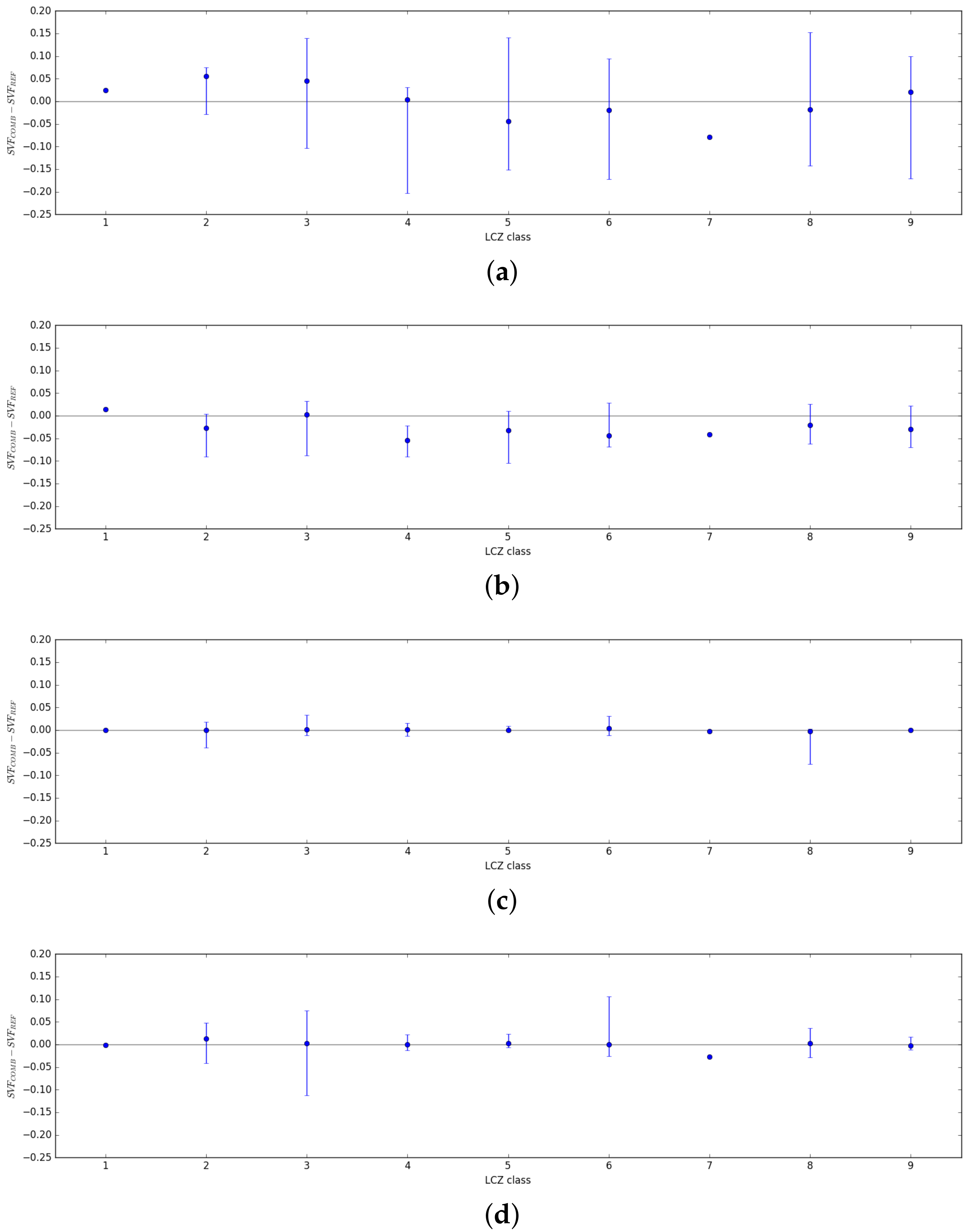
The block mean SVF error of each combination is analyzed sorting the results by LCZ built type (Figure 11), illustrated in Figure 1.
The combinations using the SAGA-GIS algorithm (C1 and C2) seems to be sensitive to the LCZ built type: the compact built types (LCZ1, 2 and 3) show higher values than the other LCZ. We have seen in Section 4.2 that the method used for the rasterization of building values affects the SAGA results: the closer the point to a building, the higher the overestimation of its SVF value. In the case of compact urban blocks, most of the grid points are located very close to a building. Thus, the SVF error obtained for such block will often be slightly higher than the one obtained for open urban blocks such as LCZ4, 5 or 6. This is especially true for combination 1 when the grid used for the SVF calculation has a high resolution (10 m). For combination 2, this overestimation is compensated by the block scale averaging described in Section 4.3: the SVF values are slightly lower than the reference SVF value for all LCZ built types.
The SVF values, calculated using the OrbisGIS algorithm combinations (C3 and C4), seem to not be impacted by the LCZ built type: there is no clear trend showing a larger or lower SVF bias for a given set of LCZ type. However, there is a higher error variability for LCZ3 and LCZ6, which are low-rise tissues, than for the others. The probability to meet a building located further than 100 m from the calculation point that may hide a part of the sky hemisphere is higher when an urban block is composed of low-rise buildings than when it is composed of high-rise buildings.
4.5. Uncertainty on the SVF Value Predicted by the Algorithms or by the Morphological Indicators
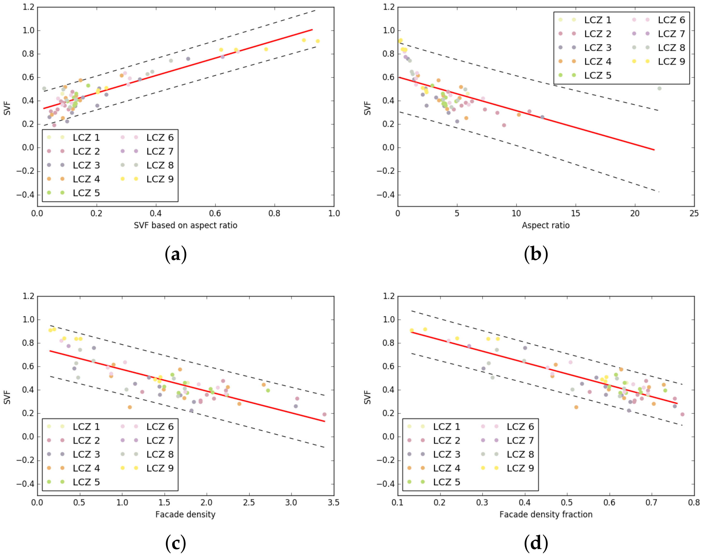
Linear relationships between and each morphological indicator are established. To improve the performances of the regression, the nine urban blocks without buildings are removed from the analysis. Indeed, a LCZ type has been attributed to each of them although they are very small. Thus, the urban blocks that surround them could have a high building density and consequently decrease the percentage of sky hemisphere visible from the empty urban block. The final formulas related to each morphological indicator are given in Equations (9) (−R² = 0.76), (9) (−R² = 0.64), (11) (−R² = 0.32) and (12) (− R² = 0.83). Note that all p-values are much lower than 0.001:
These equations may be used for SVF estimation at block scale. has the highest determination coefficient (R² = 0.83), but its formulae is not adapted for very low SVF: it is mathematically not possible to reach a SVF value under 0.318 since cannot be negative (Equation (12)). The shape of the scatter points not being linear, a logarithmic function could be used to manage this issue (Figure 12a). The same type of problem is observed for and : the SVF cannot be above 0.603 and 0.760, respectively, and the shape of the scatter is not linear (especially for –Figure 12b). On the contrary, the regression coefficient and the intercept values of Equation (9) are perfectly adapted to cover the entire range of SVF value since both are very close to 1 (or −1 for the regression coefficient). This results complement those of Bernabé et al. [16] and Groleau and Mestayer [30]: they showed that the block mean SVF can be calculated by the simple relation . In their case, the block mean SVF was calculated using roofs, facades and ground surfaces. Our results highlight that this simple relationship is still valid when the SVF is averaged only within the ground surface (note that the intensity of the relation found by Bernabé et al. [16] is similar to the one obtained herein). The second advantage of this relation is that the scatter points seem almost normally distributed around the regression line (Figure 12d).
Linear relationships have also been established between and the SVF values calculated by means of each of the combinations selected Section 4.3 (Equations (13)–(16) having respectively equal to 0.84, 0.98, 1.00, and 0.98). The objectives were to identify the potential bias related to each combination and calculate the standard error of the estimate. Note that all p-values are much lower than 0.001:
Only the combination C1 (Equation (13)) is slightly biased (low SVF values are overestimated whereas high SVF values are underestimated). The others have a negligible bias and a very high determination coefficient (). Note that all p-values are lower than 0.001.
The standard error of the estimate has been calculated for each formulae (Equations (9)–(16)); the values are gathered in Table 5.
There is a clear advantage to use the SAGA or OrbisGIS algorithms instead of the morphological indicators to accurately predict the SVF (Table 5). Except when using the combination C1, 68% of the predicted values will be within a [−0.033, 0.033] interval around the real SVF value using the software algorithms, whereas the size of the interval would double if the morphological indicators are used ([−0.073, 0.073] in the best case). However, the fastest algorithm combination (C1) has the same level of magnitude than the one calculated using or (through Equations (9) and (12)).
5. Discussion
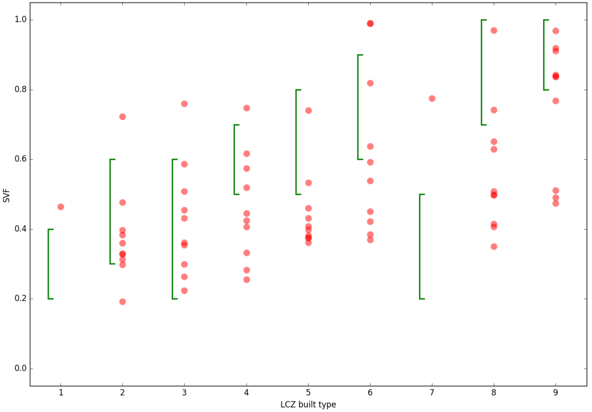
The IAUIdF did not consider the SVF indicator to attribute a LCZ built type to each urban block. It is then interesting to retrospectively verify whether their results are consistent with the SVF thresholds defined for each LCZ type. The SVF values calculated for each urban block using the OrbisGIS reference combination (Obis grid, 300 m ray length, 180 rays, 1 m grid resolution) are displayed in Figure 13. The results are splitted regarding the LCZ built type of each urban block and they are compared to the lower and upper SVF threshold proper to each LCZ type.
Most of the urban blocks classified in the LCZ 2 and 3 are within the recommended SVF interval of their class. On the contrary, for the other LCZ types, most of the urban blocks seem misclassified regarding the SVF indicator. It would then be interesting to integrate this parameter in the IAUIdF classification algorithm in order to improve their classification accuracy. For this purpose, the SVF of each of the Paris urban blocks has been calculated using the combinations C2 and C4 (cf. Section 4.3) as well as the facade density fraction (using Equation (9)). The urban blocks’ boundaries have been produced from the road network and the SVF has been calculated from building footprint and height. The corresponding data have been downloaded through the Open Data website of the city of Paris. The results obtained using the C4 combination are presented in Figure 14a since they are supposed to be the less erroneous (Table 5). In order to evaluate the accuracy of the SVF value attributed to each block, the SVF difference between the reference value and the one obtained with the C2 combination or with the facade density ratio formulae are calculated and displayed (respectively Figure 14b,c). Only the buildings located in the Paris commune territory have been considered for the SVF calculation. Then, the SVF of urban blocks located less than 100 m from the commune boundaries is considered as erroneous (these zones are not considered in the cartography).
The SVF is higher in the northern than in the southern part of Paris (Figure 14a). Much more differences can be observed in Figure 14c (between the C4 combination and method) than in Figure 14b (between the C2 and C4 combinations). Most of the differences observed in Figure 14b correspond to very densely built areas, which is consistent with the observations drawn from Figure 9: the SVF near a facade is often underestimated using SAGA. In a very dense built-up environment, most of the raster pixels are very close to a facade and then the resulting block mean SVF is underestimated. Concerning the SVF obtained using the method, it seems that they are slightly higher than the reference values in the northern part (where the SVF is high) and lower than the reference values in the southern part (where the SVF is low). This phenomenon is exacerbated for very thin blocks having no building and for large urban blocks having a very heterogeneous building distribution. Concerning the first case, the method is biased since the buildings located around the thin block are not considered for the calculation, whereas they are for the SVF calculation of the reference values (such urban blocks were removed from the analysis when establishing the linear relationships between SVF and morphological indicators). To explain the second case issue, two assumptions are proposed. The problem may come from the C4 combination: the 100 m ray length is maybe too short for such urban block configuration (e.g., the value calculated using the C4 combination was 0.1 higher than the reference value for some blocks—Figure 11d). The problem may also come from the method that would not been adapted for urban block having an heterogeneous building distribution. Further investigation is required to verify these assumptions and potentially propose a solution to fix the issue (for example, proposing a grid point distribution proper to a given urban block type).
Eventually, the computational time of each SVF calculation method can be compared: the combination C2, the combination C4 and the facade density fraction methods lasted, respectively, 18970 s, 2890 s and 250 s. Note that the processed dataset is composed of about 280000 buildings located within 9000 urban blocks. The calculation has been performed using only one core of one processor (frequency of 2.3 GHz). For the OrbisGIS case, the grid was composed of 500000 points and the time dedicated to memory access (Solid State Disk—SSD) for each point was not subtracted from the final time. The random access memory dedicated to the OrbisGIS software was 2.4 Mo.
6. Conclusions
To classify the urban fabric of a city using the LCZ classification system, the ground SVF of each zone should be known. However, the existing algorithms developed to calculate the SVF have not been evaluated at block scale. The main objective of this study was to evaluate the ability to calculate the block SVF of a raster based algorithm (SAGA-GIS) and of a vector based one (OrbisGIS). They both need two input parameters to work: the number of direction of search (or number of rays) and the distance of search (or ray length). Because the SVF is originally a point information, it should be calculated for a greater number of points to be averaged at zone scale. A grid of points linearly spaced is then used.
The vector based algorithm is found to show the best accuracy at point scale and is then considered as the reference in the rest of the study. The grid resolution affects more the SAGA-GIS values: the larger the resolution, the more the SVF is overestimated. Several combinations of number of directions, ray length and grid resolution are tested to evaluate the accuracy and computational time of each algorithm at block scale. Four of them having a relatively low error and computational time are further investigated. Four geographical indicators defining the urban morphology of an urban block are also calculated. They are used in linear regressions as explanatory variables to estimate the reference block SVF (obtained with the OrbisGIS algorithm). The main results (accuracy, computational time, bias due to a specific LCZ) of each method proposed to calculate the block SVF are summarized in Table 6.
For future LCZ classification and according to the current results, the combination C4 is recommended for the calculation of the block SVF. Cities known to have a particularly high number of blocks corresponding to LCZ 3 or 4 should draw attention since the SVF values obtained using combination C4 are then more uncertain than for other LCZ built types.
The results of this study are useful for the urban climate community. On one hand, it demonstrates the advantages of customized parameters for two algorithms available in free and open GIS: the input parameters (number of ray directions, ray length) of each algorithm can be adjusted to find a compromise between the accuracy of the expected result and the processing time. On the other hand, it shows the impact of the point grid: a raster-based algorithm is much more impacted by this parameter than a vector-based algorithm. The advantage of the vector algorithm is that the grid point distribution may be easily adapted to each urban block type (e.g., to the density of the obstacles—denser in the dense built-up blocks).
Overall, the following aspects would need further investigations:
- some of the values obtained using the SAGA software are negative. A further description and analysis of the SAGA algorithm and performance should be conducted and shared with the urban climate community.
- The nonlinearity of the relation between SVF and the indicator may be further investigated, as well as the curious simplicity of the relation between SVF and .
- All results have been produced on a limited dataset. Only the city of Paris was sampled, it would then be interesting to verify that the optimized combinations identified for the city of Paris are identical for other urban configurations and urban tissues (such as American or Asian large cities).
- The influence of the LCZ built type on the SVF calculation error has been investigated. However, the LCZ dataset used seems slightly biased regarding the SVF parameter. Very few LCZ classification algorithms have been elaborated taking into account the SVF values. This issue is addressed to the urban climate community.
- The effect of the parameter (OrbisGIS) on the computation time has been studied on a limited number of points. More investigations could be performed in order to further increase the performance of this algorithm.
Author Contributions
Conceptualization, J.B., E.B., G.P. and S.P.; Data curation, J.B. and G.P.; Formal analysis, J.B., E.B. and S.P.; Investigation, J.B., E.B. and G.P.; Methodology, J.B., E.B. and G.P.; Project administration, J.B. and E.B.; Software, J.B., E.B., G.P. and S.P.; Supervision, J.B. and E.B.; Validation, E.B.and G.P.; Visualization, J.B. and G.P.; Writing—Original draft, J.B.; Writing—Review & editing, E.B. and G.P.
Funding
This work has been funded within the following research projects frameworks: MAPuCE (Grant No. ANR-13-VBDU-0004) and URCLIM (Urban CLIMate services) framework (Grant No. 690462).
Acknowledgments
We would like to thank the producers of the data used in this work: the French National Geographical Institute (IGN) for the Paris building dataset, the Mairie de Paris for their buildings and road network open data and the Paris Region Urban and Environmental Agency for the access to their LCZ database. The English proofreading was done by Sarah Botta.
Conflicts of Interest
The authors declare no conflict of interest.
References
- Oke, T.R. Boundary Layer Climates; Routledge: Abington-on-Thames, UK, 2002. [Google Scholar]
- Jamei, E.; Rajagopalan, P.; Seyedmahmoudian, M.; Jamei, Y. Review on the impact of urban geometry and pedestrian level greening on outdoor thermal comfort. Renew. Sustain. Energy Rev. 2016, 54, 1002–1017. [Google Scholar] [CrossRef]
- Robine, J.M.; Cheung, S.L.K.; Le Roy, S.; Van Oyen, H.; Griffiths, C.; Michel, J.P.; Herrmann, F.R. Death toll exceeded 70,000 in Europe during the summer of 2003. Comptes Rendus Biol. 2008, 331, 171–178. [Google Scholar] [CrossRef] [PubMed]
- Jochner, S.; Menzel, A. Urban phenological studies–Past, present, future. Environ. Pollut. 2015, 203, 250–261. [Google Scholar] [CrossRef] [PubMed]
- Kaufmann, R.K.; Seto, K.C.; Schneider, A.; Liu, Z.; Zhou, L.; Wang, W. Climate response to rapid urban growth: evidence of a human-induced precipitation deficit. J. Clim. 2007, 20, 2299–2306. [Google Scholar] [CrossRef]
- Kolokotroni, M.; Ren, X.; Davies, M.; Mavrogianni, A. London’s urban heat island: Impact on current and future energy consumption in office buildings. Energy Build. 2012, 47, 302–311. [Google Scholar] [CrossRef]
- Sarrat, C.; Lemonsu, A.; Masson, V.; Guedalia, D. Impact of urban heat island on regional atmospheric pollution. Atmos. Environ. 2006, 40, 1743–1758. [Google Scholar] [CrossRef]
- Revel, D.; Füssel, H.M.; Jol, A. Climate Change, Impacts and Vulnerability in Europe 2012; European Economic Area (EEA): Oslo, Norway, 2012. [Google Scholar]
- Santamouris, M.; Ding, L.; Fiorito, F.; Oldfield, P.; Osmond, P.; Paolini, R.; Prasad, D.; Synnefa, A. Passive and active cooling for the outdoor built environment—Analysis and assessment of the cooling potential of mitigation technologies using performance data from 220 large scale projects. Sol. Energy 2017, 154, 14–33. [Google Scholar] [CrossRef]
- Kikegawa, Y.; Genchi, Y.; Kondo, H.; Hanaki, K. Impacts of city-block-scale countermeasures against urban heat-island phenomena upon a building’s energy-consumption for air-conditioning. Appl. Energy 2006, 83, 649–668. [Google Scholar] [CrossRef]
- Bernard, J.; Rodler, A.; Morille, B.; Zhang, X. How to Design a Park and Its Surrounding Urban Morphology to Optimize the Spreading of Cool Air? Climate 2018, 6, 10. [Google Scholar] [CrossRef]
- Ng, E.; Chen, L.; Wang, Y.; Yuan, C. A study on the cooling effects of greening in a high-density city: An experience from Hong Kong. Build. Environ. 2012, 47, 256–271. [Google Scholar] [CrossRef]
- Stewart, I.D. Redefining the Urban Heat Island. Ph.D. Thesis, University of British Columbia, Vancouver, BC, Canada, 2011. [Google Scholar]
- Stewart, I.D.; Oke, T.R. Local climate zones for urban temperature studies. Bull. Am. Meteorol. Soc. 2012, 93, 1879–1900. [Google Scholar] [CrossRef]
- Oke, T.R. Canyon geometry and the nocturnal urban heat island: comparison of scale model and field observations. Int. J. Climatol. 1981, 1, 237–254. [Google Scholar] [CrossRef]
- Bernabé, A.; Bernard, J.; Musy, M.; Andrieu, H.; Bocher, E.; Calmet, I.; Kéravec, P.; Rosant, J.M. Radiative and heat storage properties of the urban fabric derived from analysis of surface forms. Urban Clim. 2015, 12, 205–218. [Google Scholar] [CrossRef] [Green Version]
- Hämmerle, M.; Gál, T.; Unger, J.; Matzarakis, A. Comparison of models calculating the sky view factor used for urban climate investigations. Theor. Appl. Climatol. 2011, 105, 521–527. [Google Scholar] [CrossRef]
- Matzarakis, A.; Matuschek, O. Sky View Factor as a parameter in applied climatology—Rapid estimation by the SkyHelios Model. Meteorol. Z. 2011, 20, 39–45. [Google Scholar] [CrossRef]
- Zeng, L.; Lu, J.; Li, W.; Li, Y. A fast approach for large-scale Sky View Factor estimation using street view images. Build. Environ. 2018, 135, 74–84. [Google Scholar] [CrossRef]
- Kastendeuch, P.P. A method to estimate sky view factors from digital elevation models. Int. J. Climatol. 2013, 33, 1574–1578. [Google Scholar] [CrossRef]
- Chapman, L.; Thornes, J. Real-time sky-view factor calculation and approximation. J. Atmos. Ocean. Technol. 2004, 21, 730–741. [Google Scholar] [CrossRef]
- Unger, J. Connection between urban heat island and sky view factor approximated by a software tool on a 3D urban database. Int. J. Environ. Pollut. 2008, 36, 59–80. [Google Scholar] [CrossRef]
- Chen, L.; Ng, E.; An, X.; Ren, C.; Lee, M.; Wang, U.; He, Z. Sky view factor analysis of street canyons and its implications for daytime intra-urban air temperature differentials in high-rise, high-density urban areas of Hong Kong: A GIS-based simulation approach. Int. J. Climatol. 2012, 32, 121–136. [Google Scholar] [CrossRef]
- Böhner, J.; McCloy, K.R.; Strobl, J. SAGA: Analysis and Modelling Applications; Number 115; Goltze: Gottingen, Germany, 2006. [Google Scholar]
- Bocher, E.; Petit, G. OrbisGIS: Geographical Information System designed by and for research. In Innovative Software Development in GIS; Wiley: Hoboken, NJ, USA, 2013; pp. 23–66. [Google Scholar]
- Cordeau, E. Les îLots Morphologiques Urbains (IMU). 2016. Available online: https://www.iau-idf.fr/savoir-faire/nos-travaux/edition/les-ilots-morphologiques-urbains-imu.html (accessed on 3 July 2018).
- Bocher, E.; Petit, G.; Fortin, N.; Palominos, S. H2GIS a spatial database to feed urban climate issues. In Proceedings of the 9th International Conference on Urban Climate (ICUC9), Toulouse, France, 20–24 July 2015. [Google Scholar]
- Gál, T.; Lindberg, F.; Unger, J. Computing continuous sky view factors using 3D urban raster and vector databases: Comparison and application to urban climate. Theor. Appl. Climatol. 2009, 95, 111–123. [Google Scholar] [CrossRef]
- Bocher, E.; Petit, G.; Bernard, J.; Palominos, S. A geoprocessing framework to compute urban indicators: The MApUCE tools chain. Urban Clim. 2018, 24, 153–174. [Google Scholar] [CrossRef]
- Groleau, D.; Mestayer, P.G. Urban Morphology Influence on Urban Albedo: A Revisit with the S olene Model. Bound.-Layer Meteorol. 2013, 147, 301–327. [Google Scholar] [CrossRef]
Figure 1.
Abridged definitions for LCZ built types. Source: Stewart and Oke [14]—©American Meteorological Society, used with permission.
Figure 1.
Abridged definitions for LCZ built types. Source: Stewart and Oke [14]—©American Meteorological Society, used with permission.

Figure 2.
Selected 10 Paris urban blocks by LCZ type (defined Figure 1) and the corresponding buildings located within a 300 m radius. Based on the LCZ database produced by the IAUIdF. Note that the LCZ corresponding to each urban block has been colored at the 300 m buffer scale in order to make them identifiable.

Figure 3.
Calculation of the approximated surface hemisphere (blue) hidden by the buildings’ obstacles (red) in a given direction (green line). In this example, the hemisphere is split into height sectors (number of directions) and the surface of the hemisphere considered as hidden by the buildings in the given direction is shown in grey.

Figure 4.
General data flow of the study.

Figure 5.
The SAGA-GIS and OrbisGIS grids and the corresponding buildings used for the SVF calculation.
Figure 5.
The SAGA-GIS and OrbisGIS grids and the corresponding buildings used for the SVF calculation.

Figure 6.
Building configuration for the analytical solution calculation: (a) configuration 1: circularly extruded building; (b) configuration 2: street canyon.
Figure 6.
Building configuration for the analytical solution calculation: (a) configuration 1: circularly extruded building; (b) configuration 2: street canyon.

Figure 7.
Scheme of the raster-based approach (SAGA software) for the configuration 1–scenario 1. The squares represent the pixels of the raster: the blue ones are considered as building surfaces, the white ones as ground surfaces. The SVF is calculated from the pixel covered by the pink circle.
Figure 7.
Scheme of the raster-based approach (SAGA software) for the configuration 1–scenario 1. The squares represent the pixels of the raster: the blue ones are considered as building surfaces, the white ones as ground surfaces. The SVF is calculated from the pixel covered by the pink circle.

Figure 8.
Effect of the input parameters value on the SVF difference recorded at point scale using OrbisGIS or SAGA-GIS algorithm: (a) grid resolution; (b) ray length; and (c) number of directions. The red line is the median point, the upper and lower box limits are, respectively, the first and third quartiles and the lower and upper whisker are the 5 and 95 percentiles.

Figure 9.
SVF difference between SAGA and OrbisGIS values.

Figure 10.
Block mean SVF error versus processing time duration using (a) SAGA-GIS algorithm and SAGA grid; (b) OrbisGIS algorithm and SAGA grid; and (c) OrbisGIS algorithm and Orbis grid. The marker is the median value of the 72 blocks and the whiskers are the lower and upper quartile.
Figure 10.
Block mean SVF error versus processing time duration using (a) SAGA-GIS algorithm and SAGA grid; (b) OrbisGIS algorithm and SAGA grid; and (c) OrbisGIS algorithm and Orbis grid. The marker is the median value of the 72 blocks and the whiskers are the lower and upper quartile.

Figure 11.
Block mean SVF error regarding the LCZ built type for (a) combination C1; (b) combination C2; (c) combination C3; and (d) combination C4. The blue dot represents the median SVF error, the blue segment is the range of the SVF error. Based on the LCZ database produced by the IAUIdF.
Figure 11.
Block mean SVF error regarding the LCZ built type for (a) combination C1; (b) combination C2; (c) combination C3; and (d) combination C4. The blue dot represents the median SVF error, the blue segment is the range of the SVF error. Based on the LCZ database produced by the IAUIdF.

Figure 12.
Relationship between block mean SVF value calculated using the reference algorithm combination and (a) canyon street SVF; (b) aspect ratio; (c) facade density; and (d) facade density fraction. The red line is the regression line and the dotted-lines represent the 95% prediction interval. Based on the LCZ database produced by the IAUIdF.

Figure 13.
Urban block SVF values (red dots) splitted by LCZ built type and their corresponding SVF lower and upper threshold (green segments), based on the LCZ database produced by the IAUIdF.
Figure 13.
Urban block SVF values (red dots) splitted by LCZ built type and their corresponding SVF lower and upper threshold (green segments), based on the LCZ database produced by the IAUIdF.

Figure 14.
SVF of the Paris urban blocks: (a) values obtained using combination C4; (b) difference between the values obtained using combination C2 and the ones using combination C4; and (c) difference between the values obtained using the facade density ratio formulae and the ones using combination C4.


Table 1.
Value range of each parameter tested herein.
| Parameter to Evaluate | Values to Test |
|---|---|
| Ray length (m) | 100, 200, 300 |
| Number of directions | 60, 120, 180 |
| Grid resolution (m) | 1, 2, 5, 10 |
Table 2.
Geometric dimensions for each combination of configuration/scenarios.
| Scenario | Configuration 1 | Configuration 2 | |||
|---|---|---|---|---|---|
| 1 | 20 m | 39 m | 20 m | 39 m | 2000 m |
| 2 | 20 m | 40 m | 20 m | 40 m | 2000 m |
Table 3.
Morphological indicator definition.
| Notation | Name | Description | Formulae | Reference |
|---|---|---|---|---|
| Facade density | The building external free facades area () is divided by the block surface () | Bocher et al. [29] | ||
| Facade density fraction | The building external free facades area is divided by the block surface plus the building free facades area | Bernabé et al. [16] | ||
| Aspect ratio | The street canyon definition is extended to any urban tissue using the ratio of the building external free facades and the land free surface (urban block area minus building footprint area–) | - | ||
| Canyon street SVF | The SVF is calculated using the aspect ratio considering all the streets of the urban block as street canyons | Oke [15] |
Table 4.
SVF values calculated for each combination of method (algorithm or analytical solution), scenario and building configuration.
Table 4.
SVF values calculated for each combination of method (algorithm or analytical solution), scenario and building configuration.
| Scenario | Building Configuration | OrbisGIS | SAGA-GIS | Analytical Solution |
|---|---|---|---|---|
| 1 | 1 (circular courtyard) | 0.50000 (≃0%) | 0.50000 (=0%) | 0.5 |
| 2 (street canyon) | 0.70713 (+0.004%) | 0.70608 (−0.15%) | 0.70711 | |
| 2 | 1 (circular courtyard) | 0.52199 (≃0%) | 0.52438 (+0.45%) | 0.52199 |
| 2 (street canyon) | 0.72252 (+0.003%) | 0.71993 (−0.35%) | 0.72249 |
(%) the number given inside the parenthesis is the relative error percentage.
Table 5.
Predicted SVF block uncertainty for each of the methods presented herein.
| Method | Morphological Indicators | Algorithm Combinations | ||||||
|---|---|---|---|---|---|---|---|---|
| C1 | C2 | C3 | C4 | |||||
| Standard deviation of the estimate | 0.087 | 0.107 | 0.147 | 0.073 | 0.085 | 0.033 | 0.014 | 0.027 |
Table 6.
lMain results summary.
| Name | C1 | C2 | C3 | C4 | |||||
|---|---|---|---|---|---|---|---|---|---|
| Method | Type | SAGA GIS | SAGA GIS | Orbis GIS | Orbis GIS | Morpho indic | Morpho indic | Morpho indic | Morpho indic |
| ND | 180 | 60 | 60 | 60 | - | - | - | - | |
| RL (m) | 300 | 100 | 100 | 100 | - | - | - | - | |
| GR (m) | 10 | 2 | 5 | 10 | - | - | - | - | |
| Results | OK | OK | OK | OK | Non normal residuals | OK | Non normal residuals | Non normal residuals | |
| Particular LCZ bias | LCZ1, 2 & 3 | LCZ1, 2 & 3 | No | No | - | - | - | - | |
| Particular LCZ uncertainty | No | No | No | LCZ3 & 6 | - | - | - | - | |
| Stand. dev. estimate | 0.085 | 0.033 | 0.014 | 0.027 | 0.087 | 0.107 | 0.147 | 0.073 | |
| Comput. time for Paris (s) | - | 18,970 | - | 2890 | - | 250 | - | - | |
© 2018 by the authors. Licensee MDPI, Basel, Switzerland. This article is an open access article distributed under the terms and conditions of the Creative Commons Attribution (CC BY) license (http://creativecommons.org/licenses/by/4.0/).
Share and Cite
MDPI and ACS Style
Bernard, J.; Bocher, E.; Petit, G.; Palominos, S. Sky View Factor Calculation in Urban Context: Computational Performance and Accuracy Analysis of Two Open and Free GIS Tools. Climate 2018, 6, 60. https://doi.org/10.3390/cli6030060
AMA Style
Bernard J, Bocher E, Petit G, Palominos S. Sky View Factor Calculation in Urban Context: Computational Performance and Accuracy Analysis of Two Open and Free GIS Tools. Climate. 2018; 6(3):60. https://doi.org/10.3390/cli6030060
Chicago/Turabian StyleBernard, Jérémy, Erwan Bocher, Gwendall Petit, and Sylvain Palominos. 2018. "Sky View Factor Calculation in Urban Context: Computational Performance and Accuracy Analysis of Two Open and Free GIS Tools" Climate 6, no. 3: 60. https://doi.org/10.3390/cli6030060
Note that from the first issue of 2016, this journal uses article numbers instead of page numbers. See further details here.